
A Wolf Pack Optimization Algorithm Using RASGS and GBA for Multi-Modal Multi-Objective Problems

1
School of Mechanical Electronic & Information Engineering, China University of Mining & Technology-Beijing, Beijing 100083, China
2
R & D Department, Zhuhai Xinhe Technology Co., Ltd., Zhuhai 519000, China
3
School of Electrical Engineering, Zhejiang University, Hangzhou 310000, China
*
Author to whom correspondence should be addressed.
Symmetry 2022, 14(12), 2568; https://doi.org/10.3390/sym14122568
Submission received: 11 November 2022
/
Revised: 28 November 2022
/
Accepted: 2 December 2022
/
Published: 5 December 2022
Abstract
:To address multi-modal multi-objective problems (MMOPs), this paper proposes a wolf pack optimization algorithm using random adaptive-shrinking grid search (RASGS) and raid towards global best archive (GBA) for MMOPs. Firstly, RASGS with logical symmetry was adopted to enhance the exploitation of the algorithm in the local area as well as locate a larger number of Pareto-optimal solutions. Moreover, with the help of an existing sorting method composed of the non-dominated sorting scheme and special crowding distance (SCD), the GBA strategy was employed to obtain and maintain the historical global optimal solution of the population as well as induce the population to explore better solutions. The experimental results indicate that the proposed method has obvious superior performance compared with the existing related algorithms.
1. Introduction
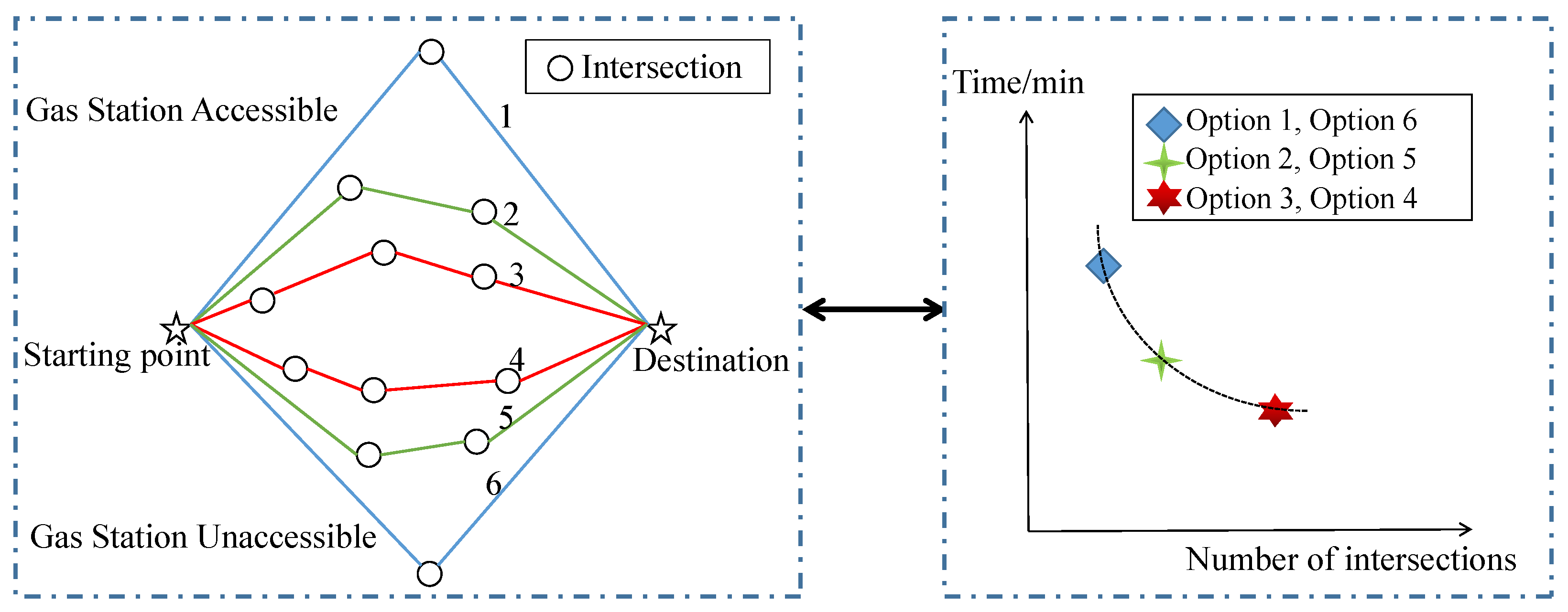
In many practical problems, such as economic, management, military, science and engineering design, it is often difficult to judge the quality of a scheme with one index, and more than one uncoordinated or even contradictory objectives must be considered simultaneously. Multi-modal multi-objective optimization problems are defined as the multi-objective optimization problems (MOPs) with at least two similar feasible regions in the decision space corresponding to the same region of the objective space [1]. In real life, it is critical to find all the Pareto optimal solutions in decision space simultaneously for the purpose of decision-making as well as a new challenge; for instance, it is in [2] that the researchers described a real-world scenario: {Option 1, Option 2, Option 3} and {Option4, Option 5, Option 6} are two Pareto sets (PSs) that correspond to the same Pareto front (PF); however, the former go through a gas station while the latter do not. The gas station is needed for some travelers, while it is unnecessary and a nuisance with some potential safety risks for the others, as detailed in Figure 1.
People have been active in researching and solving multi-objective problems to meet various emerging needs, such as in [3], where to solve constrained MOPs (CMOPs), Zou et al. proposed a dual population multi-objective optimization evolutionary algorithm that is different from the traditional MOPs. In [4], to solve global optimization problems regarding multiple objective functions, Moghdani R et al. introduced the multi-objective volleyball premier league (MOVPL) algorithm. In [5], Ewees A.A. et al. reported a new multi-objective optimization method (called MWDEO) including improved whale optimization algorithm (WOA) devoted to global exploration as well as the differential evolution (DE) algorithm used to exploit the search space, which enriches the theoretical research in this field. Wang Q et al. adopted multi-objective optimization methods to solve the problems regarding aerospace shell production scheduling in [6]. In [7], researchers proposed a novel particle swarm optimization method named AMPSO by combining dynamic neighborhood-based learning strategy and competition mechanism, committing to solve MMOPs. In [8], researchers introduced a novel and efficient method for solving MOPs inspired by the collision between balls in the game of billiards. In [9], researchers presented a test suite for MOPs including 16 real-world problems, which is used for performance evaluation for multiple-objective optimization algorithms. Some papers showed surveys for methods to solve MOPs, such as in [10], where researchers systematically reviewed and summarized various multi-objective methods devoted to solving MOPs based on hundreds of articles published from 1978 to 2021. In [11], Tian Y et al. gave a comprehensive overview of multi-objective evolutionary algorithms to solve large-scale MOPs.
Recently, the wolf pack optimization algorithm (WPOA) and its variants have been widely applied in many fields owing to their superior optimization performance and robustness. For example, in [12], a novel algorithm named FWPA is proposed to solve a set of static multidimensional knapsack benchmarks as well as several dynamic multidimensional knapsack problems. In [13], researchers adopted a new wolf pack algorithm named HWPA to improve the forecasting performance by obtaining a suitable partition of the universe of discourse. In [14], the authors proposed a new method named DSO-WPOA to promote the coverage rate of movable wireless sensor networks. Especially, in [15], the authors proposed a strategy named ASGS to promote the exploitation ability in local space, which greatly enhances the optimization ability of the WPOA.
Unfortunately, there are few cases where the WPOA or its variants are used to solve MMOPs. Consequently, inspired by the superior performance of the WPOA and the need to address MMOPs, in this paper we propose a wolf pack optimization algorithm using random adaptive-shrinking grid search (RASGS) and raid towards global best archive (GBA) for multi-modal multi-objective problems (MMO-WPOA-RASGS-GBA for short).
2. Related Works
2.1. Special Crowding Distance and non-dominated_scd_sort
It is hard to decide which solution is the best one in multi-objective optimization owing to its complexity discussed above, so a dominated relationship [16] was designed to compare the qualities of different solutions which lead to the new concepts: non-dominated solutions, the Pareto optimal set (PS) in decision space as well as the corresponding Pareto front (PF) in objective space [1].
To analyze and manipulate the distribution of the various Pareto optimal sets, researchers proposed the concept of a crowding distance (CD), which is embedded in the omni-optimizer algorithm [17] to compare different non-dominated schemes. Accordingly, the idea of CD has been applied to the following related algorithms, for example, in [1], aiming to obtain more PSs, Liang et al. introduced DN-NSGAII, which utilizes a decision-space CD to sort the same front in objective space, which means the CD of PSs in the decision space can be used to determine which solution is better.
where means the CD of the i-th solution in j-th decision space, while means the one in m-th objective space; means the total CD of the i-th solution in decision space, while means the one in objective space; Num_D means the dimension number of decision space, while Num_O means the one of objective space.
It should be emphasized that the calculation of CD is different in the decision space and the objective space, and for decision space CD can be obtained from Equation (1) and for objective space from Equation (2). Note that if a solution is a boundary solution in the decision space, the numerator in Equation (1) should be replaced by () or (), as the case may be, and the quantity should be multiplied by a factor of two since this computes only a one-sided difference; otherwise, when a solution is a boundary solution in the objective space, an infinite distance is assigned so as not to lose the solution.
where means the average CD of all solutions in objective space; Num_S means the number of all solutions.
However, CD has shortcomings in that if a solution i is the smallest one in the m-th objective for minimization problems, is set to ∞, and is equal to ∞, so it is unable to compare the and . Accordingly, in [2], researchers proposed special crowding distance (SCD) conceived for the purpose of further improving CD along with an obvious adaptation that is assigned to be set to 1 when the i-th solution is the minimum one in the m-th objective space for minimization problems. The SCD can be obtained from the following Equation (4).
where SCDi means the special crowding distance of the i-th solution; CDi,x means the crowding distance of the i-th solution about decision space, while CDi,f means the one about objective space. max(parameter1,parameter2) is a function that returns the parameter with a larger value, while max(parameter1,parameter2) returns the one with a smaller value.
According to the original authors, SCD enhanced genetic diversity of both decision and objective spaces simultaneously owing to the max or min selection procedure reflected in Equation (4).
non-dominated_scd_sort is a function based on non-dominated relation and SCD, which firstly sorts solutions according to non-dominated sorting scheme from Reference [18] and then sorts them in descending order according to their SCD, with the result that the first solution is the non-dominated one with the largest SCD. In fact, non-dominated_scd_sort provides a reference to compare the quality of many different non dominated solutions, which provides support for the GBA strategy discussed later in this paper.
2.2. Strategy of Adaptive-Shrinking Grid Search (ASGS)
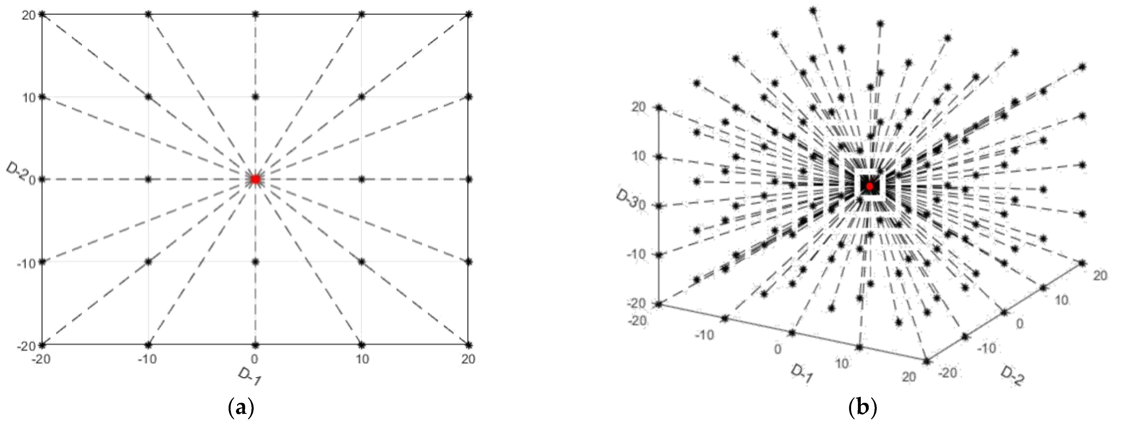
In 2007, researchers introduced the wolf swarm algorithm [19] inspired by the hunting process of wolves and composed mainly of the migration, summon-raid, siege, and population renewal mechanism of survival of the fittest. Since the wolf pack optimization algorithm (WPOA) was proposed, it has been widely applied in many different kinds of fields and continuously improved in various forms owing to its strong performance detailed in [15]. As a variant of the WPOA, the excellent performance of ASGS-CWOA [15] mainly benefits from the strategy of ASGS, which inspired us to use it to solve MMOPs. It is briefly described as follows.
Based on the ideas of LWPS [20] and CWOA [21], only one position was examined to determine whether it can become the next traveling position, shown in Equation (5); that is, a searching wolf can investigate one position along a direction, and it is obvious that the method is not suitable for searching for the local neighborhood space centered by the current wolf, which includes numerous locations to be investigated.
where xid−new means the new location of the i-th wolf about the d-th dimension; rand(−1,1) returns a random value between −1 and 1; step_a means the step size during the stage of migration.
Thus, in [15], the authors proposed the strategy of ASGS conceived for the purpose of covering the whole local domain space centered by the current wolf to be investigated as much as possible, although it is impossible to exhaust all the positions to be investigated for the continuous space problem. The main thought of ASGS is to take the current wolf position as the center and the changing adaptive step size as the measurement scale to generate several inspection points in order to detect the best position in the local region (the position with the best fitness value) for the procedure of migration or siege, as shown in the following Equations (6) and (7).
where is a factor for step_anew and step_cnew; step_anew means the new step size of migration for the t-th iteration, while step_cnew means the one of siege; rand(0,1) returns a random value between 0 and 1; step_c0 means the initial step size of the stage of siege; K means the number of nodes taken along any direction for a wolf; xi−new means the new position of i-th wolf while xid−new means the new one for the d-th dimension.
3. Overview of New Proposed Method
3.1. RASGS
It is difficult to solve the MMP problem, while the ASGS greatly improves the optimization performance of the wolf pack optimization algorithm when solving the single objective problem. This encourages us to use the modified ASGS-CWOA to solve the MMP problem. It is undeniable that ASGS-CWOA has excellent performance in solving MMPs (as demonstrated in the experiment in Section 4).
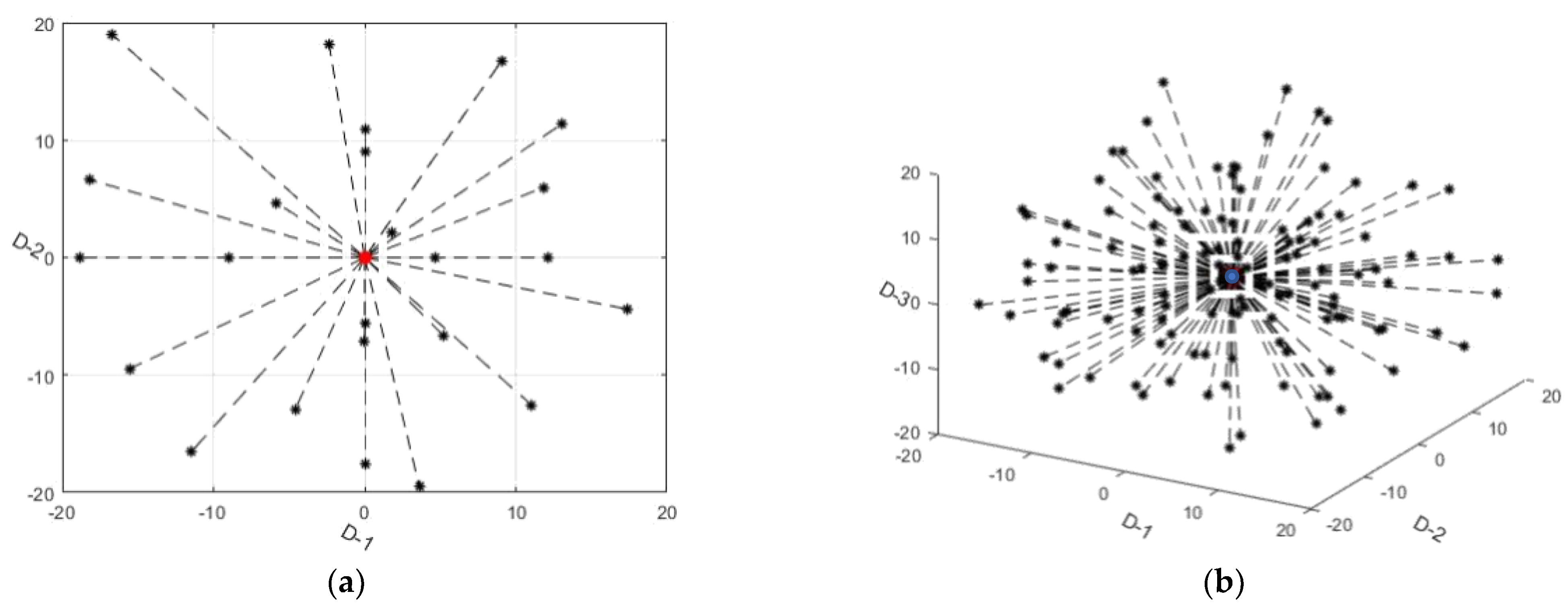
However, we also found that the ASGS strategy extends with the same step size. Although the step size changes adaptively with the advance of iterations, this equidistant expansion greatly limits the flexibility of the ASGS strategy as shown in Figure 2. In order to overcome this deficiency of the ASGS strategy, we propose the random ASGS strategy (RASGS) that introduces a random parameter in the equidistant step size to make the ASGS strategy flexible while maintaining its own basic exploration/extension framework as shown in Figure 3. In Figure 2 and Figure 3, the red point indicates the location of the current wolf, while the black ones represent the positions to be investigated during the stage of migration or siege, and the black dotted lines indicate the potential routes for the current wolf to explore. The RASGS strategy can be illustrated by the following Equation (8).
where the variables involved in Equation (8) can be found in the formula already described.
In essence, solving nonlinear and irregular MMPs requires that the algorithm can not only maintain the stability of the search framework in the hunting and siege stages but also maintain a certain degree of flexibility to deal with the complex and infinite solution space. RASGS inherits the function of the former and introduces random parameters resulting in the implementation of the latter. Similar to ASGS-CWOA, the algorithm based on this new strategy is abbreviated to RASGS-CWOA.
It can also be seen from Figure 3 that although random factors have been added, the locations to be investigated in the local areas are symmetrical and centered on the current wolf position, which is determined by Formula (8).
3.2. GBA
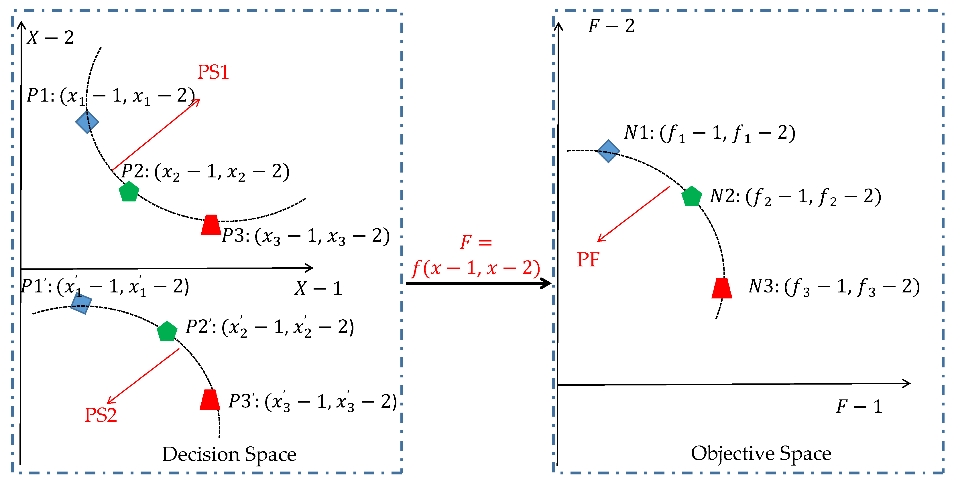
As mentioned above, MMPs have multiple inconsistent goals, making it impossible to compare the quality of different non-dominated solutions through traditional methods, so a global optimal solution like the single objective programming problem cannot be found, as shown in the Figure 4 where for N1, N2 and N3, the best solution cannot be compared due to the two independent evaluation objectives F-1 and F-2. Obviously, solution N1 (corresponding to P1 and P1′ in the decision space) is the best on target F-2 and the worst on F-1 (assuming the larger the better). On the contrary, solution N3 (corresponding to P3 and P3′ in the decision space) is the worst on target F-2 and the best on F-1. Solution N2 (corresponding to P2 and p2′ in the decision space) is in the middle value on objectives F-1 and F-2.
In [2], the authors adopted SCD to sort the non-dominated solutions so as to obtain a descending order of non-dominated solutions that could not be compared before. The first non-dominated solution in the sequence has the optimal SCD.
According to the idea of ASGS-CWOA, wolves need to raid to the leader wolf; that is, the global optimum, in the summon-raid stage, and the non-dominated solution sorting method proposed in Reference [2] provides the necessary method for obtaining the global optimum required in this stage. In fact, the first non-dominated solution in the sequence obtained after sorting is not really the global optimum in the true sense but a reference, which is enough to induce wolves to gather. In this paper, the method based on SCD to obtain the global optimum and complete the calculation of the summon-raid is called raid to global best archive (GBA) as shown in Figure 5.
In particular, in order to compare the support of the GBA strategy for the methods proposed in this paper, this paper proposes the strategy of raid to neighborhood best (RNB for short) based on previous studies, the main idea of which is to establish the local neighborhood optimal archive centered on the current wolf (this paper adopts the ring strategy taking N−1, N and N+1, where N means the current solution while N−1 and N+1 mean the solution before the current solution and the one after the current solution, respectively, detailed in Reference [2]). In the summon-raid stage, wolves rush to the optimal one in their respective neighborhood optimal archive, not the one with the global optimum.
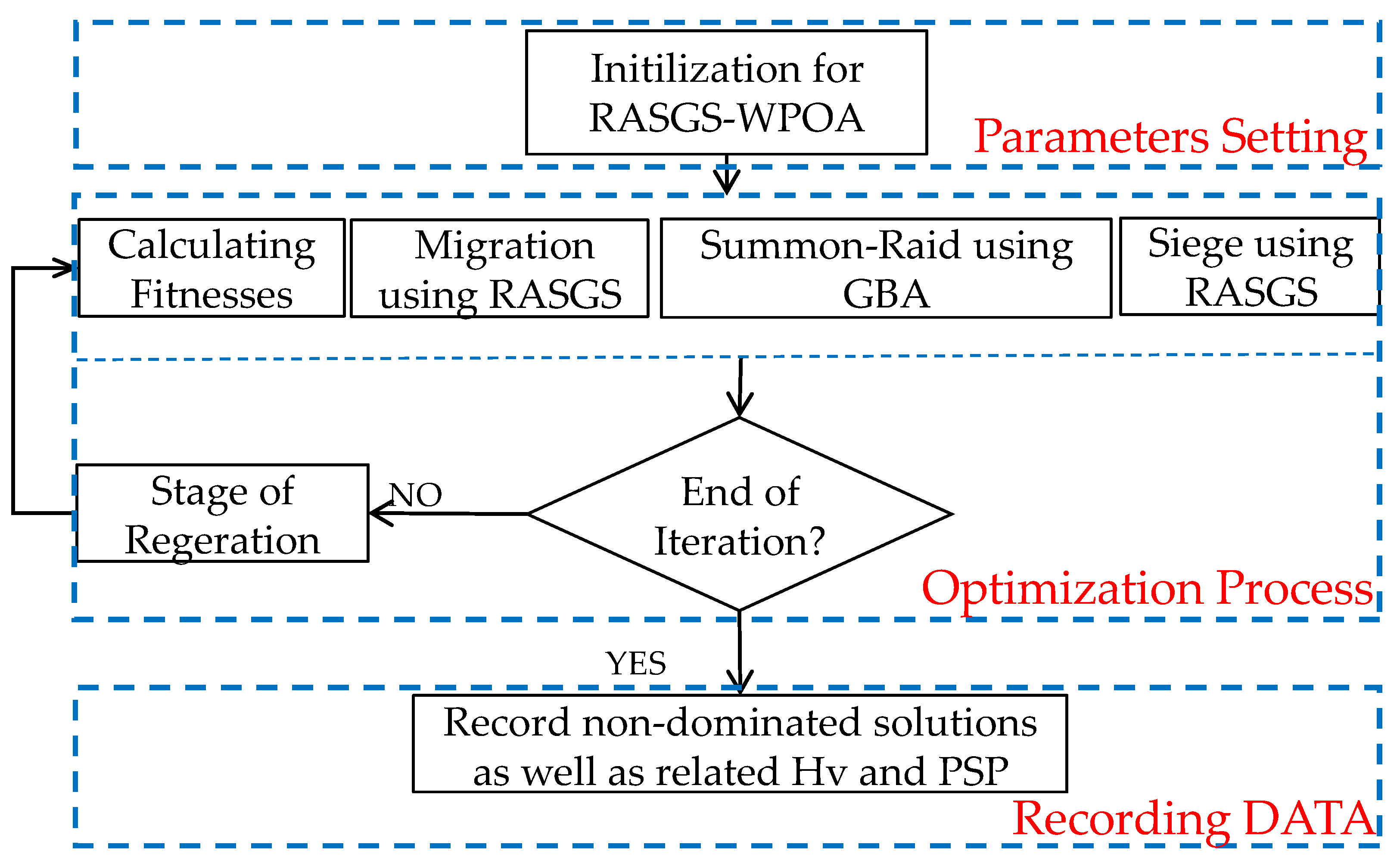
3.3. Overview of Flow Chart of MMO-WPOA-RASGS-GBA
The execution flow of the new algorithm is shown in Figure 5, and the detailed operation details are as described above as well as referring to Reference [15], while the step size during stages of migration, summon-raid and siege are calculated according to Equations (9) and (10).
where stepa, stepb and stepc mean the step size during stages of migration, summon-raid and siege, respectively. VRmax is the maximum range of solution space, while VRmin means the minimum one in each dimension.
4. Validation Experiment
4.1. Experimental Environment
To verify the feasibility and efficiency of the algorithm proposed in this paper, several groups of comparative experiments were carried out by using the new method: MMO-WPOA-RASGS-GBA, DN-NSGAII, MO-Ring-PSO-SCD, MMO-WPOA-LWPS-GBA, MMO-WPOA-LWPS-RNB, MMO-WPOA-ASGS-GBA, MMO-WPOA-ASGS-RNB and MMO-WPOA-RASGS-RNB. A detailed description is given in the following Table 1.
Table 1 shows the numerical experimental configuration and concepts of the eight methods. We conducted all the experiments on a laptop with Windows 7 (64 bit), 12.0 GB memory and an AMD A6-3400 m CPU. In order to meet the following statistical analysis needs, independent experiments were carried out 21 times on 11 test functions as shown in Table 2.
4.2. Experimental Data and Analysis
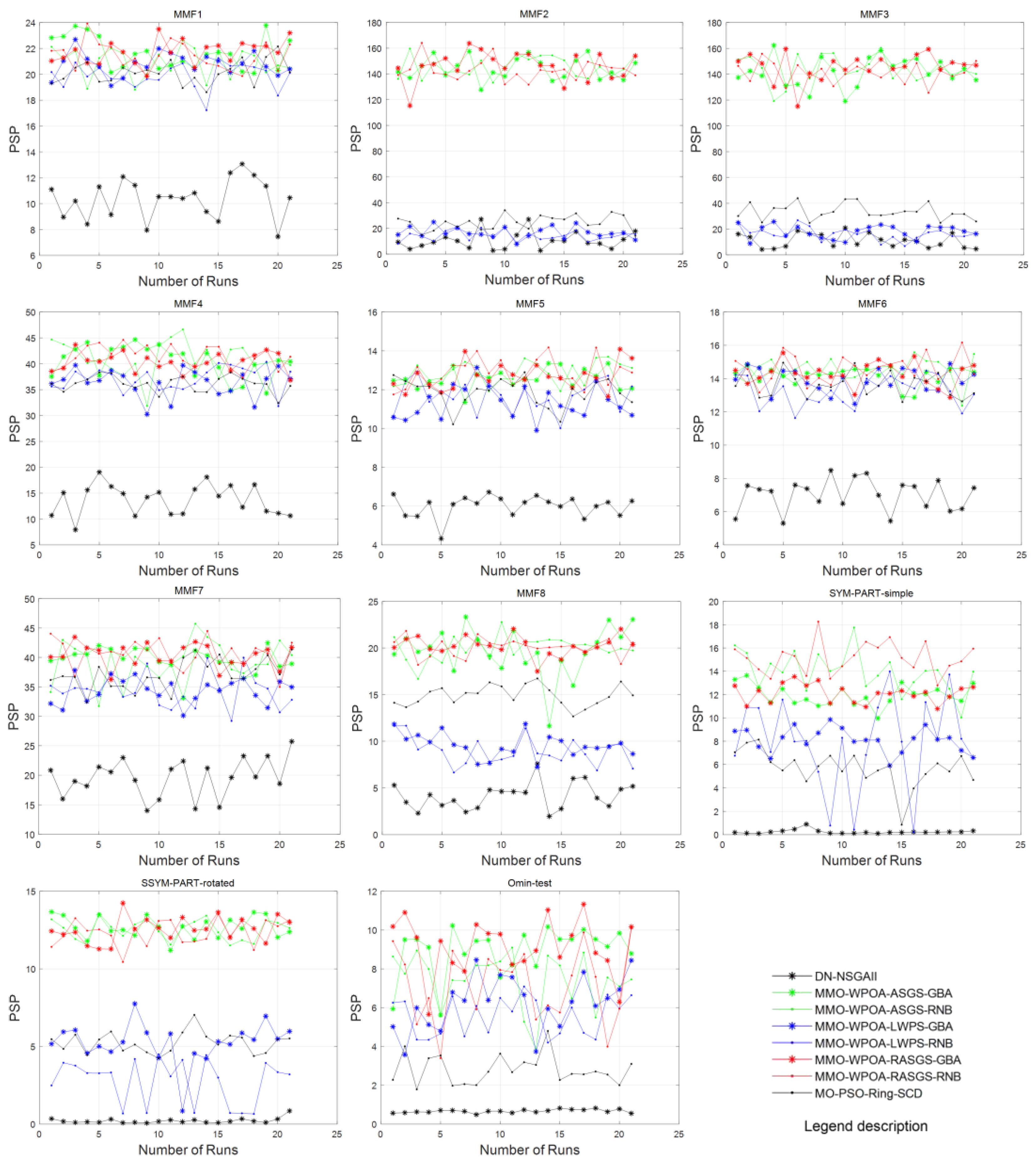
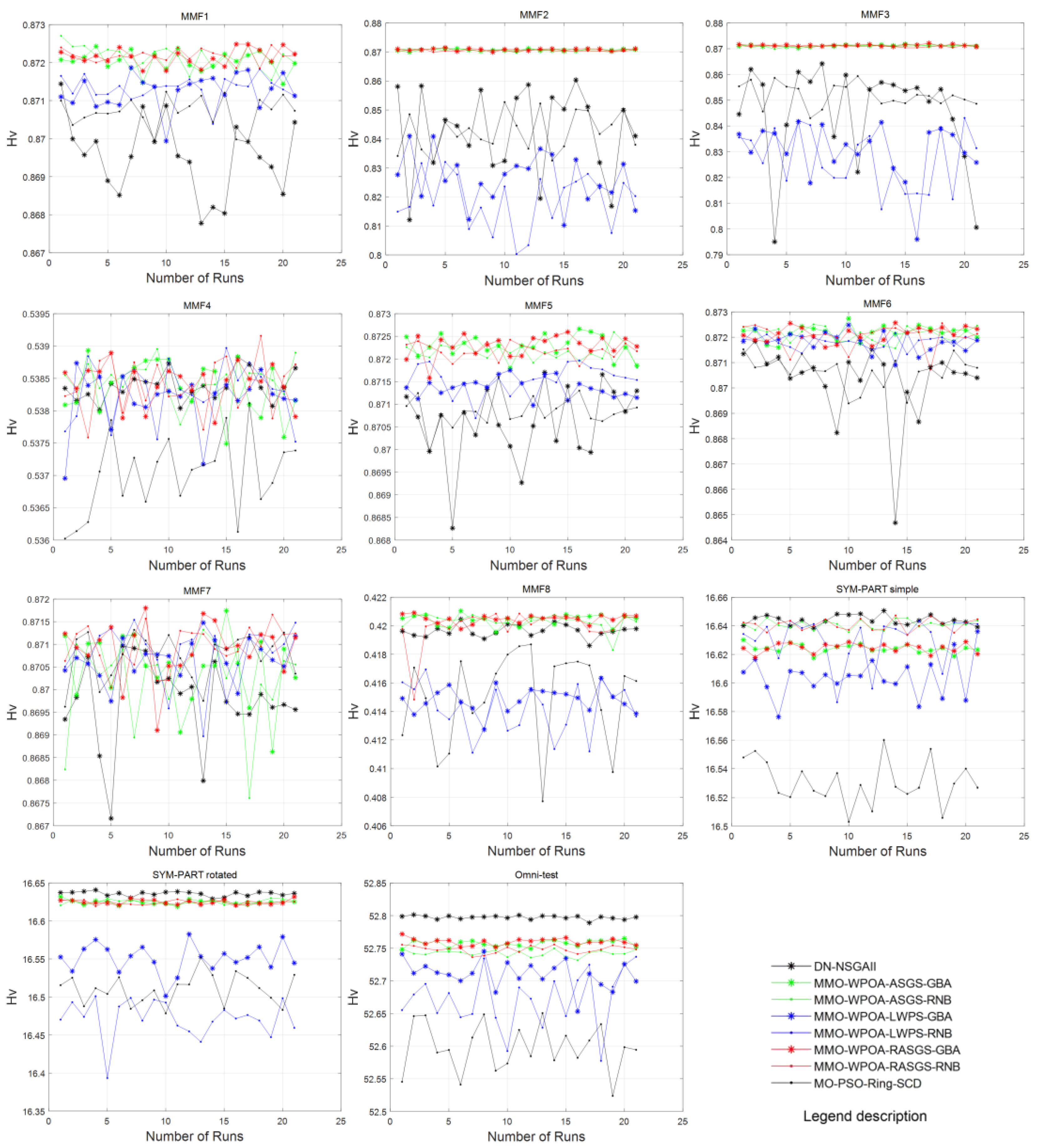
In this study, Pareto set proximity (PSP) and hypervolume (Hv) were adopted to test the performance of different methods for MMPs. For a detailed introduction of PSP and HV, please refer to Reference [2]. In order to facilitate simulation experiments and statistics, we used the reciprocal forms of PSP and HV: rPSP and rHV, the smaller the better. On 11 test functions, 21 simulation experiments were carried out for 8 comparison algorithms, and the original data obtained from the experiments are shown in Table 3, which gives the original test data regarding PSP gained by running each comparison algorithm on 11 test functions as well as the data regarding HV. Based on these original test data, some necessary analysis and discussion regarding the performance of different methods are given.
Note: black “*” corresponds to DN-NSGAII; black “.” corresponds to MO-PSO-Ring-SCD; green “*” corresponds to MMO-WPOA-ASGS-GBA; green “.” corresponds to MMO-WPOA-ASGS-RNB; blue “*” corresponds to MMO-WPOA-LWPS-GBA; blue “.” corresponds to MMO-WPOA-LWPS-RNB; red “*” corresponds to MMO-WPOA-RASGS-GBA and red “.” corresponds to MMO-WPOA-RASGS-RNB. Refer to Figure 6 and Figure 7.
As can be seen from Figure 6 and Figure 7, it is obvious that the red * curve representing the new method MMO-WPOA-RASGS-GBA is at the top except for the last three subgraphs of Figure 7, which shows that this method has good performance on the whole based on PSP and HV indicators.
However, we can also see that green curves and the red “.” curve representing MMO-WPOA-ASGS-RNB, MMO-WPOA-ASGS-GBA and MMO-WPOA-RASGS-RNB are very close, so it is hard to distinguish their performance based on Figure 6 and Figure 7. Accordingly, optimal value, worst value, average value and the standard deviation for PSP and HV are adopted to help us further investigate and analyze the superior performance of the new algorithm, shown in Table 4.
Table 5 was obtained based on the values listed in Table 4 to show the dominance ratios between the newly proposed algorithm and other similar algorithms for PSP and HV.
In terms of the optimal value or maximum value of PSP, it can be clearly seen from Table 5 that six records of MMO-WPOA-RASGS-GBA are better than MMO-WPOA-ASGS-GBA, five records are better than MMO-WPOA-ASGS-RNB and four records are better than MMO-WPOA-RASGS-RNB, and the difference between other records without advantages is very small. In particular, the former has the best performance in the more complex functions SYM-PART-rotated and Omni-test (with 9 and 27 Pareto sets, respectively, as detailed in Table 2). In terms of minimum or worst value for PSP, seven records of MMO-WPOA-RASGS-GBA are better than MMO-WPOA-ASGS-GBA, seven records are better than MMO-WPOA-ASGS-RNB and four records are better than MMO-WPOA-RASGS-RNB, and the difference between other records without advantages is very small, which means that the proposed method
MMO-WPOA-RASGS-GBA has an advantage rate of about 63.64%, 63.64% and 36.36% compared with the other three approximation algorithms. Similarly, in terms of median for PSP, nine records of MMO-WPOA-RASGS-GBA are better than MMO-WPOA-ASGS-GBA, seven records are better than MMO-WPOA-ASGS-RNB and six records are better than MMO-WPOA-RASGS-RNB, and the difference between other records without advantages is very small, which means that MMO-WPOA-RASGS-GBA has an advantage rate of about 81.82%, 63.64% and 54.55% compared with the other three approximation algorithms. Finally, in terms of standard deviation for PSP, six records of MMO-WPOA-RASGS-GBA are better than MMO-WPOA-ASGS-GBA, seven records are better than MMO-WPOA-ASGS-RNB and eight records are better than MMO-WPOA-RASGS-RNB, and the difference between other records without advantages is very small, which means that MMO-WPOA-RASGS-GBA has an advantage rate of about 54.55%, 63.64% and 72.73% compared with the other three approximation algorithms.
Therefore, it can be concluded that the proposed algorithm has overall advantages in terms of PSP index.
In terms of the optimal value or maximum value of HV, it can be clearly seen from Table 5 that five records of MMO-WPOA-RASGS-GBA are better than MMO-WPOA-ASGS-GBA, eight records are better than MMO-WPOA-ASGS-RNB and nine records are better than MMO-WPOA-RASGS-RNB, and the difference between other records without advantages is very small, which means that MMO-WPOA-RASGS-GBA has an advantage rate of about 45.45%, 72.73% and 81.82% compared with the other three approximation algorithms. In terms of minimum or worst value for HV, nine records of MMO-WPOA-RASGS-GBA are better than MMO-WPOA-ASGS-GBA, nine records are better than MMO-WPOA-ASGS-RNB and six records are better than MMO-WPOA-RASGS-RNB, and the difference between other records without advantages is very small, which means that the proposed method MMO-WPOA-RASGS-GBA has an advantage rate of about 81.82%, 81.82% and 54.55% compared with the other three approximation algorithms. Similarly, in terms of median for HV, nine records of MMO-WPOA-RASGS-GBA are better than MMO-WPOA-ASGS-GBA, seven records are better than MMO-WPOA-ASGS-RNB and eight records are better than MMO-WPOA-RASGS-RNB, and the difference between other records without advantages is very small, which means that MMO-WPOA-RASGS-GBA has an advantage rate of about 81.82%, 63.64% and 72.73% compared with the other three approximation algorithms. Correspondingly, in terms of standard deviation for HV, five records of MMO-WPOA-RASGS-GBA are better than MMO-WPOA-ASGS-GBA, six records are better than MMO-WPOA-ASGS-RNB and six records are better than MMO-WPOA-RASGS-RNB, and the difference between other records without advantages is very small, which means that MMO-WPOA-RASGS-GBA has an advantage rate of about 45.45%, 54.55% and 54.55% compared with the other three approximation algorithms.
Accordingly, it can be concluded that the proposed algorithm has overall advantages in terms of HV index, although some performance is not good.
5. Conclusions
To address multi-modal multi-objective problem, a wolf pack optimization algorithm using strategies of random adaptive-shrinking grid search and raid towards global best for MMOPs is proposed, which enriches the method system for using the WPOA to solve MMOPs and makes two key contributions: Firstly, RASGS was adopted to enhance the exploitation of the algorithm in the local area as well as locate a larger number of Pareto-optimal solutions. Moreover, with the help of an existing sorting method composed of the non-dominated sorting scheme and SCD, the strategy of GBA is introduced to obtain and maintain the historical global optimal solution of the population as well as induce the population to explore better solutions. Theoretical research and experimental results indicate that MMO-WPOA-RASGS-GBA has comprehensively superior PSP and HV compared with DN-NSGAII, MO-Ring-PSO-SCD, MMO-WPOA-LWPS-GBA, MMO-WPOA-LWPS-NBA, MMO-WPOA-ASGS-GBA, MMO-WPOA-ASGS-NBA and MMO-WPOA-RASGS-NBA under the same conditions.
However, it needs to be stated that MMO-WPOA-RASGS-GBA is not perfect, and its performance is not optimal in some aspects, such as MMO-WPOA-RASGS-RNB performing better than MMO-WPOA-RASGS-GBA on maximum and minimum values of PSP, as shown in Table 5, which indicates the strategy of RNB is better than GBA in some aspects. Unfortunately, the former performs weakly on median and standard deviation of PSP. On the contrary, this is exactly the advantage of the method proposed in this paper.
Future work will be carried out to continuously improve our related methods to address MMOPs and solve practical engineering problems.
Author Contributions
H.W. and D.W. conceived the algorithm framework and wrote the paper; D.W. and H.W. performed the program experiments; D.W. contributed the data. All authors have read and agreed to the published version of the manuscript.
Funding
This study is funded by the National Key Research and Development Program of China (grant no. SQ2018YFC060172).
Data Availability Statement
The complete data including PSP and HV obtained from the experiments are shown in the link in Appendix A.
Acknowledgments
The authors are grateful to peer experts for their full support of this paper and thank China University of Mining & Technology-Beijing, as well as Zhuhai Xinhe Technology Co., Ltd., which provided the necessary scientific research environment.
Conflicts of Interest
The authors declare no conflict of interest.
Appendix A
Extraction Code: 3133.
References
- Liang, J.J.; Yue, C.T.; Qu, B.Y. Multimodal multi-objective optimization: A preliminary study. In Proceedings of the 2016 IEEE Congress on Evolutionary Computation (CEC), Vancouver, BC, Canada, 24–29 July 2016. [Google Scholar] [CrossRef]
- Yue, C.; Qu, B.; Liang, J. A multi-objective particle swarm optimizer using ring topology for solving multimodal multi-objective problems. IEEE Trans. Evol. Comput. 2017, 22, 805–817. [Google Scholar] [CrossRef]
- Zou, J.; Sun, R.; Yang, S.; Zheng, J. A dual-population algorithm based on alternative evolution and degeneration for solving constrained multi-objective optimization problems. Inf. Sci. 2021, 579, 89–102. [Google Scholar] [CrossRef]
- Moghdani, R.; Salimifard, K.; Demir, E.; Benyettou, A. Multi-objective volleyball premier league algorithm. Knowl. Based Syst. 2020, 196, 105781. [Google Scholar] [CrossRef]
- Ewees, A.A.; Elaziz, M.A.; Oliva, D. A new multi-objective optimization algorithm combined with opposition-based learning. Expert Syst. Appl. 2021, 165, 113844. [Google Scholar] [CrossRef]
- Wang, Q.; Wang, X.; Luo, H.; Xiong, J. An Improved Multi-Objective Evolutionary Approach for Aerospace Shell Production Scheduling Problem. Symmetry 2020, 12, 509. [Google Scholar] [CrossRef] [Green Version]
- Zhang, X.W.; Liu, H.; Tu, L.P. A modified particle swarm optimization for multimodal multi-objective optimization. Eng. Appl. Artif. Intell. 2020, 95, 103905. [Google Scholar] [CrossRef]
- Moghaddam, M.R.; Khanzadi, M.; Kaveh, A. Multi-objective Billiards-Inspired Optimization Algorithm for Construction Management Problems. Iran. J. Sci. Technol. Trans. Civ. Eng. 2021, 45, 2177–2200. [Google Scholar] [CrossRef]
- Tanabe, R.; Ishibuchi, H. An easy-to-use real-world multi-objective optimization problem suite. Appl. Soft Comput. 2020, 89, 106078. [Google Scholar] [CrossRef]
- Karimi, N.; Feylizadeh, M.R.; Govindan, K.; Bagherpour, M. Fuzzy multi-objective programming: A systematic literature review. Expert Syst. Appl. 2022, 196, 116663. [Google Scholar] [CrossRef]
- Tian, Y.; Si, L.; Zhang, X.; Cheng, R.; He, C.; Tan, K.C.; Jin, Y. Evolutionary Large-Scale Multi-Objective Optimization: A Survey. ACM Comput. Surv. 2021, 54, 1–34. [Google Scholar] [CrossRef]
- Wu, H.; Xiao, R. Flexible Wolf Pack Algorithm for Dynamic Multidimensional Knapsack Problems. Research 2020, 2020, 1762107. [Google Scholar] [CrossRef] [PubMed] [Green Version]
- Xian, S.; Li, T.; Cheng, Y. A Novel Fuzzy Time Series Forecasting Model Based on the Hybrid Wolf Pack Algorithm and Ordered Weighted Averaging Aggregation Operator. Int. J. Fuzzy Syst. 2020, 22, 1832–1850. [Google Scholar] [CrossRef]
- Wang, D.; Wang, H.; Ban, X.; Qian, X.; Ni, J. An Adaptive, Discrete Space Oriented Wolf Pack Optimization Algorithm for a Movable Wireless Sensor Network. Sensors 2019, 19, 4320. [Google Scholar] [CrossRef] [PubMed] [Green Version]
- Wang, D.; Ban, X.; Ji, L.; Guan, X.; Liu, K.; Qian, X. An Adaptive Shrinking Grid Search Chaotic Wolf Optimization Algorithm Using Standard Deviation Updating Amount. Comput. Intell. Neurosci. 2020, 2020, 7986982. [Google Scholar] [CrossRef] [PubMed]
- Konak, A.; Coit, D.W.; Smith, A.E. Multi-objective optimization using genetic algorithms: A tutorial. Reliab. Eng. Syst. Saf. 2006, 91, 992–1007. [Google Scholar] [CrossRef]
- Deb, K.; Tiwari, S. Omni-optimizer: A procedure for single and multi-objective optimization. In Proceedings of the International Conference on Evolutionary Multi-Criterion Optimization, Guanajuato, Mexico, 9–11 March 2005; pp. 47–61. [Google Scholar]
- Deb, K.; Pratap, A.; Agarwal, S.; Meyarivan, T. A fast and elitist multiobjective genetic algorithm: NSGA-II. IEEE Trans. Evol. Comput. 2002, 6, 182–197. [Google Scholar] [CrossRef] [Green Version]
- Yang, C.; Tu, X.; Chen, J. Algorithm of marriage in honey bees optimization based on the wolf pack search. In Proceedings of the 2007 International Conference on Intelligent Pervasive Computing (IPC 2007), Jeju, Republic of Korea, 11–13 October 2007; pp. 462–467. [Google Scholar]
- Zhou, Q.; Zhou, Y.Q. Wolf colony search algorithm based on leader strategy. Appl. Res. Comput. 2013, 30, 2629–2632. [Google Scholar]
- Zhu, Y.; Jiang, W.; Kong, X.; Quan, L.; Zhang, Y. A chaos wolf optimization algorithm with self-adaptive variable step-size. AIP Adv. 2017, 7, 105024. [Google Scholar] [CrossRef]
Figure 1.
Path planning problem. Option 1, Option 6—1 intersection, 60 min; Option 2, Option 5—2 intersections, 40 min; Option 3, Option 4—3 intersections, 20 min.
Figure 1.
Path planning problem. Option 1, Option 6—1 intersection, 60 min; Option 2, Option 5—2 intersections, 40 min; Option 3, Option 4—3 intersections, 20 min.

Figure 2.
Schematic of the ASGS strategy. (a) Schematic when Dimension is 2 and K is set to 2 for Equation (7). (b) Schematic when Dimension is 3 and K is set to 3.(Red point means the current locaton while the black ones mean the locations to be inspected).
Figure 2.
Schematic of the ASGS strategy. (a) Schematic when Dimension is 2 and K is set to 2 for Equation (7). (b) Schematic when Dimension is 3 and K is set to 3.(Red point means the current locaton while the black ones mean the locations to be inspected).

Figure 3.
Schematic of the RASGS strategy. (a) Schematic when Dimension is 2 and K is set to 2 for Equation (7). (b) Schematic when Dimension is 3 and K is set to 3. (Both red point and blue point mean the current location while the black ones mean the ones to be inspected).
Figure 3.
Schematic of the RASGS strategy. (a) Schematic when Dimension is 2 and K is set to 2 for Equation (7). (b) Schematic when Dimension is 3 and K is set to 3. (Both red point and blue point mean the current location while the black ones mean the ones to be inspected).

Figure 4.
Schematic of non-dominated solutions. Here, PS means Pareto sets, while PF means Pareto front, and P1, P1′—N1, P2, P2′—N2 and P3, P3′—N3.
Figure 4.
Schematic of non-dominated solutions. Here, PS means Pareto sets, while PF means Pareto front, and P1, P1′—N1, P2, P2′—N2 and P3, P3′—N3.

Figure 5.
Flow chart of MMO-WPOA-RASGS-GBA.

Figure 6.
Schematic diagram of the PSP obtained from 21 independent runs.

Figure 7.
Schematic diagram of the HV obtained from 21 independent runs.


Table 1.
Descriptions of comparative methods.
| Order | Name | Description |
|---|---|---|
| 1 | MMO-WPOA-RASGS-GBA | MMO-WPOA-RASGS-GBA was implemented according to the ideas from Section 2 and Section 3 and with the following main parameters. Population size: popsize = 100 × n_var (n_var means the number of dimension in decision space); maximum iterations: Max_Gen = fix (5000 × n_var/popsize), where fix is a function that rounds a given parameter to the nearest integer in the direction of zero. |
| 2 | DN-NSGAII | According to the idea from Reference [1], DN-NSGII was designed and implemented. |
| 3 | MO-Ring-PSO-SCD | For comparison, the algorithm MO-Ring-PSO-SCD was completely implemented by using the ideas of Reference [2], and the code and data published by the author were fully used. |
| 4 | MMO-WPOA-LWPS-GBA | MMO-WPOA-LWPS-GBA was implemented based on LWPS and the strategy of GBA, where LWPS is the concept of Reference [20]. In order to maintain the consistency of comparison, the main parameter settings were the same as the new proposed method MMO-WPOA-RASGS-GBA. |
| 5 | MMO-WPOA-LWPS-RNB | MMO-WPOA-LWPS-RNB was implemented based on LWPS and the strategy of RNB. The main parameter settings were the same as the new proposed method MMO-WPOA-RASGS-GBA. |
| 6 | MMO-WPOA-ASGS-GBA | MMO-WPOA-ASGS-GBA was implemented based on ASGS-CWOA and the strategy of GBA. The main parameter settings were the same as the new proposed method MMO-WPOA-RASGS-GBA. |
| 7 | MMO-WPOA-ASGS-RNB | MMO-WPOA-ASGS-RNB was implemented based on ASGS-CWOA and the strategy of RNB. The main parameter settings were the same as the new proposed method MMO-WPOA-RASGS-GBA. |
| 8 | MMO-WPOA-RASGS-RNB | MMO-WPOA-RASGS-RNB was implemented based on RASGS-CWOA and the strategy of RNB. The main parameter settings were the same as the new proposed method MMO-WPOA-RASGS-GBA. |
Table 2.
Test functions and their features.
| Function Name | Numbers of PSs | Overlap in Every Dimension |
|---|---|---|
| MMF1 | 2 | ✗ |
| MMF2 | 2 | ✗ |
| MMF3 | 2 | ✓ |
| MMF4 | 4 | ✗ |
| MMF5 | 4 | ✗ |
| MMF6 | 4 | ✓ |
| MMF7 | 2 | ✗ |
| MMF8 | 4 | ✗ |
| SYM-PART simple | 9 | ✓ |
| SYM-PART rotated | 9 | ✓ |
| Omni-test (n = 3) | 27 | ✓ |
Table 3.
PSP and HV obtained from running 8 comparison algorithms on 11 test functions.
| Method | Function | Best | Worst | Mean | Standard Deviation | ||||
|---|---|---|---|---|---|---|---|---|---|
| PSP | HV | PSP | HV | PSP | HV | PSP | HV | ||
| DN-NSGAII | 1 | 13.07157454 | 0.871441292 | 7.45420489 | 0.867777461 | 10.37862956 | 0.869543972 | 1.537400748 | 0.000971016 |
| 2 | 27.14697376 | 0.86034517 | 2.743265272 | 0.812130676 | 10.66215106 | 0.842723622 | 7.025888613 | 0.014772512 | |
| 3 | 20.99165336 | 0.864179667 | 4.321204324 | 0.795025678 | 11.03379399 | 0.845174252 | 5.389567687 | 0.019247749 | |
| 4 | 19.06053311 | 0.538831423 | 7.920388234 | 0.538013489 | 13.74047358 | 0.538371962 | 2.963817426 | 0.000223549 | |
| 5 | 6.721691985 | 0.871705041 | 4.318902002 | 0.868264371 | 6.003089379 | 0.870574743 | 0.554027273 | 0.000831438 | |
| 6 | 8.487121963 | 0.871841635 | 5.297196162 | 0.864684655 | 7.018860458 | 0.870276462 | 0.944228126 | 0.001536351 | |
| 7 | 25.73434643 | 0.870961261 | 14.03144506 | 0.867162762 | 19.59652068 | 0.869747436 | 3.233112307 | 0.000948028 | |
| 8 | 7.574435284 | 0.420461536 | 1.968899546 | 0.418607833 | 4.165918029 | 0.419632606 | 1.41998449 | 0.000424649 | |
| 9 | 0.901421457 | 16.65058558 | 0.102172245 | 16.63836026 | 0.248497916 | 16.64395359 | 0.174115453 | 0.003450843 | |
| 10 | 0.851985453 | 16.64076529 | 0.071600353 | 16.62908329 | 0.217284248 | 16.63583674 | 0.171143405 | 0.00305863 | |
| 11 | 0.824966497 | 52.80128767 | 0.490736377 | 52.78893019 | 0.669547795 | 52.79724749 | 0.089073764 | 0.00288194 | |
| ...... | Related data for MO-Ring-PSO-SCD, MMO-WPOA-LWPS-GBA, MMO-WPOA-LWPS-RNB, MMO-WPOA-ASGS-GBA, MMO-WPOA-ASGS-RNB, MMO-WPOA-RASGS-GBA | ||||||||
| MMO-WPOA-RASGS-RNB | 1 | 23.93129451 | 0.872464015 | 19.78287453 | 0.871847053 | 21.41931497 | 0.872185149 | 1.080976338 | 0.000170628 |
| 2 | 164.1425286 | 0.871207671 | 131.6933317 | 0.869951014 | 143.0823892 | 0.870452374 | 7.876139977 | 0.000293692 | |
| 3 | 155.8376542 | 0.871516532 | 125.5565595 | 0.870361056 | 141.025033 | 0.870966491 | 7.632984748 | 0.000359212 | |
| 4 | 44.61290138 | 0.539158648 | 37.32542416 | 0.537586604 | 41.39526592 | 0.538390431 | 2.136074745 | 0.000416678 | |
| 5 | 14.17445297 | 0.872425458 | 11.75215944 | 0.871841708 | 12.87865508 | 0.872182454 | 0.733297984 | 0.000160872 | |
| 6 | 16.16825152 | 0.872555153 | 13.16557559 | 0.870727596 | 14.60809281 | 0.872027625 | 0.801278727 | 0.000459748 | |
| 7 | 44.49262842 | 0.87165644 | 34.98611381 | 0.870040226 | 40.65581559 | 0.870956842 | 2.399970212 | 0.000453174 | |
| 8 | 21.84212415 | 0.420854555 | 18.19303417 | 0.414828247 | 20.09382787 | 0.419980567 | 0.968923642 | 0.001257179 | |
| 9 | 18.27235864 | 16.64725864 | 12.79305015 | 16.63366917 | 15.15875804 | 16.6406475 | 1.345772599 | 0.003929908 | |
| 10 | 13.51032998 | 16.62859054 | 10.44428702 | 16.619417 | 12.33495567 | 16.62457421 | 0.808215646 | 0.002706662 | |
| 11 | 10.08414621 | 52.75576581 | 3.400506796 | 52.73641053 | 7.186849936 | 52.74821071 | 1.866408547 | 0.005407196 | |
(1-MMF1, 2-MMF2, 3-MMF3, 4-MMF4, 5-MMF5, 6-MMF6, 7-MMF7, 8-MMF8, 9-SYM_PART_simple, 10-SYM-PART-rotated, 11-Omni-test. Limited to space, only some data are listed; the complete data are shown in the link in Appendix A).
Table 4.
Difference between MMO-WPOA-RASGS-GBA and other similar methods.
| Item | Order | Difference from PSP | Difference from HV | ||||||
|---|---|---|---|---|---|---|---|---|---|
| Best | Worst | Mean | SD | Best | Worst | Mean | SD | ||
| MMO-WPOA-RASGS-GBA vs. MMO-WPOA-ASGS-GBA | 1 | −0.286 | −0.201 | 0.084 | −0.353 | 0.000058 | 0.000342 | 0.000115 | −0.000045 |
| 2 | 5.941 | −12.345 | 2.047 | 2.514 | 0.000284 | −0.000023 | 0.000130 | 0.000023 | |
| 3 | −2.777 | −4.035 | 4.173 | −1.272 | 0.000314 | 0.000453 | 0.000189 | 0.000008 | |
| 4 | −0.990 | 2.557 | −0.108 | −1.307 | −0.000037 | 0.000320 | 0.000061 | −0.000110 | |
| 5 | 0.729 | 0.299 | 0.111 | 0.154 | −0.000069 | −0.000219 | 0.000008 | −0.000010 | |
| 6 | 0.736 | −0.006 | 0.083 | 0.171 | −0.000173 | 0.000001 | −0.000058 | 0.000011 | |
| 7 | 0.981 | 3.152 | 0.790 | −0.204 | 0.000058 | 0.000475 | 0.000441 | −0.000149 | |
| 8 | −1.288 | 5.861 | 0.549 | −1.618 | −0.000131 | 0.000218 | 0.000071 | −0.000108 | |
| 9 | −0.099 | 0.822 | 0.153 | −0.099 | −0.001311 | 0.000372 | 0.000426 | 0.000230 | |
| 10 | 0.566 | 0.082 | −0.141 | 0.087 | −0.000035 | 0.001645 | −0.000159 | 0.000284 | |
| 11 | 1.103 | 0.032 | 0.192 | 0.187 | 0.006698 | 0.003756 | 0.002740 | 0.000001 | |
| MMO-WPOA-RASGS-GBA vs. MMO-WPOA-ASGS-NBA | 1 | 0.869 | 1.060 | 0.804 | −0.231 | −0.000221 | 0.000235 | 0.000014 | −0.000087 |
| 2 | 4.089 | −17.950 | 0.862 | 3.338 | 0.000265 | 0.000293 | 0.000148 | −0.000040 | |
| 3 | −0.817 | −4.143 | 2.317 | −0.095 | 0.000322 | 0.000828 | 0.000234 | −0.000070 | |
| 4 | −2.946 | 4.975 | −0.724 | −1.425 | −0.000059 | 0.000023 | −0.000037 | 0.000043 | |
| 5 | 0.388 | −0.272 | −0.197 | 0.102 | 0.000002 | −0.000229 | 0.000138 | 0.000063 | |
| 6 | −0.034 | 0.495 | −0.234 | −0.013 | 0.000061 | 0.000034 | −0.000001 | 0.000002 | |
| 7 | −2.262 | 4.520 | 0.982 | −1.514 | 0.000478 | 0.001490 | 0.000664 | −0.000318 | |
| 8 | −0.728 | 0.804 | 0.244 | −0.238 | 0.000040 | 0.001471 | 0.000181 | −0.000241 | |
| 9 | −4.212 | 0.752 | −1.848 | −0.934 | −0.016784 | −0.017689 | −0.016462 | 0.000119 | |
| 10 | 0.660 | −0.231 | 0.031 | 0.134 | 0.001701 | 0.001232 | −0.000149 | −0.000082 | |
| 11 | 2.238 | 1.786 | 1.685 | 0.049 | 0.021988 | 0.019958 | 0.017610 | 0.000246 | |
| MMO-WPOA-RASGS-GBA vs. MMO-WPOA-RASGS-NBA | 1 | −0.430 | 0.090 | 0.308 | −0.172 | 0.000022 | −0.000070 | −0.000037 | 0.000048 |
| 2 | −0.358 | −16.393 | 3.237 | 3.359 | 0.000282 | −0.000012 | 0.000376 | 0.000080 | |
| 3 | 3.775 | −10.517 | 4.956 | 2.424 | 0.000630 | 0.000341 | 0.000359 | −0.000005 | |
| 4 | −0.922 | −0.487 | −1.063 | −0.329 | −0.000263 | 0.000223 | 0.000031 | −0.000111 | |
| 5 | −0.087 | −0.102 | −0.198 | −0.062 | 0.000170 | −0.000264 | 0.000111 | 0.000079 | |
| 6 | −0.619 | −0.299 | −0.322 | −0.107 | 0.000016 | 0.000874 | 0.000099 | −0.000172 | |
| 7 | −1.023 | 1.259 | −0.300 | −0.466 | 0.000146 | −0.000937 | −0.000057 | 0.000160 | |
| 8 | 0.218 | −0.697 | 0.156 | 0.068 | 0.000057 | 0.004944 | 0.000502 | −0.000967 | |
| 9 | −4.721 | −2.007 | −3.041 | −0.560 | −0.018404 | −0.015793 | −0.016118 | −0.000714 | |
| 10 | 0.730 | 0.834 | 0.218 | −0.016 | 0.003227 | 0.001239 | 0.000091 | 0.000453 | |
| 11 | 1.251 | 2.255 | 1.949 | −0.427 | 0.016015 | 0.015172 | 0.011846 | −0.000418 | |
(1-MMF1, 2-MMF2, 3-MMF3, 4-MMF4, 5-MMF5, 6-MMF6, 7-MMF7, 8-MMF8, 9-SYM-PART-Simple, 10-SYM-PART-rotated, 11-Omni-test).
Table 5.
Statistical data for MMO-WPOA-RASGS-GBA and other similar methods.
| Item | Index | Statistics for PSP | Statistics for HV | ||
|---|---|---|---|---|---|
| Number of Advantages | Dominance Ratio (Total: 11) | Number of Advantages | Dominance Ratio (Total: 11) | ||
| vs. MMO-WPOA-ASGS-GBA | Best | 6 | 54.55% | 5 | 45.45% |
| Worst | 7 | 63.64% | 9 | 81.82% | |
| Mean | 9 | 81.82% | 9 | 81.82% | |
| SD | 6 | 54.55% | 5 | 45.45% | |
| vs. MMO-WPOA-ASGS-NBA | Best | 5 | 45.45% | 8 | 72.73% |
| Worst | 7 | 63.64% | 9 | 81.82% | |
| Mean | 7 | 63.64% | 7 | 63.64% | |
| SD | 7 | 63.64% | 6 | 54.55% | |
| vs. MMO-WPOA-RASGS-NBA | Best | 4 | 36.36% | 9 | 81.82% |
| Worst | 4 | 36.36% | 6 | 54.55% | |
| Mean | 6 | 54.55% | 8 | 72.73% | |
| SD | 8 | 72.73% | 6 | 54.55% | |
Publisher’s Note: MDPI stays neutral with regard to jurisdictional claims in published maps and institutional affiliations. |
© 2022 by the authors. Licensee MDPI, Basel, Switzerland. This article is an open access article distributed under the terms and conditions of the Creative Commons Attribution (CC BY) license (https://creativecommons.org/licenses/by/4.0/).
Share and Cite
MDPI and ACS Style
Wang, H.; Wang, D. A Wolf Pack Optimization Algorithm Using RASGS and GBA for Multi-Modal Multi-Objective Problems. Symmetry 2022, 14, 2568. https://doi.org/10.3390/sym14122568
AMA Style
Wang H, Wang D. A Wolf Pack Optimization Algorithm Using RASGS and GBA for Multi-Modal Multi-Objective Problems. Symmetry. 2022; 14(12):2568. https://doi.org/10.3390/sym14122568
Chicago/Turabian StyleWang, Huibo, and Dongxing Wang. 2022. "A Wolf Pack Optimization Algorithm Using RASGS and GBA for Multi-Modal Multi-Objective Problems" Symmetry 14, no. 12: 2568. https://doi.org/10.3390/sym14122568
Note that from the first issue of 2016, this journal uses article numbers instead of page numbers. See further details here.