Strain Monitoring-Based Fatigue Assessment and Remaining Life Prediction of Stiff Hangers in Highway Arch Bridge

Abstract

The fatigue problem of hangers is fatal for the safety of the whole bridge structure. The objective of this study is to present a strain monitoring-based method to assess the fatigue performance of stiff hangers in highway arch bridges and predict their remaining life. A vehicle–bridge interaction system was constructed to analyze the dynamic behavior in the area close to the key welding line where the hanger was connected to the deck slab. Then, the empirical mode decomposition (EMD) algorithm and rain-flow counting algorithm were used in signal preprocessing and statistical analysis of field monitoring data. Finally, the fatigue life was assessed according to the standards in the Chinese Code for the Design of Steel Structures, as well as the Eurocode 3 and AASHTO codes. Differences were found in the fatigue behavior of hangers, and the shortest hanger was shown to surfer more serious fatigue damage. The influence of vehicle volume growth and low-stress amplitude on the fatigue performance was also discussed.

1. Introduction

Hangers are crucial structural members in half-through or through arch bridges, in which the hangers transfer structural dead weight and traffic loads to the arch rib. A series of collapse accidents of arch bridges (Yibin Nanmen Bridge, Nanfang’ao Bridge, etc.) caused by the fatigue performance failure of hangers have caused widespread concern. Therefore, considerable efforts have been made in the past decades to reveal the deterioration mechanism of hangers and evaluate their serving conditions. However, the existing studies mainly focused on a discussion of the fatigue behavior of the steel strand hanger [1,2,3,4]. Another type of hanger, namely, the stiff hanger, is also widely applied in many bridges. H-section, circular-section, thick-plate, and hollow-box-section steel members represent common structural forms of stiff hangers. García and Jorquera [5] analyzed the structural longitudinal performance of a tied-arch bridge with stiff hangers, and provided some advice to reduce the bending moment at the end zones of the deck. Zhong et al. [6,7] conducted a fatigue assessment of short stiff hangers in Nanjing Da Sheng Guan Bridge using the dynamic strain under train loads. In particular, few studies have considered the fatigue performance of stiff hangers in highway arch bridges.

With the application of structure health monitoring technology, fatigue assessment methods can directly utilize the monitoring data to obtain evaluation indicators [8,9,10,11,12,13,14,15,16,17,18]. Li and Zhu [14] presented a long-term condition assessment approach for hangers in the Tsing Ma cable-suspension bridge under in-service traffic loads based on structural monitoring techniques. Liu et al. [15] proposed a stochastic time-variant reliability assessment method for corrosion fatigue analysis of short hangers in suspension and arch bridges. Chen [16] carried out a fatigue performance assessment of composite arch bridge hangers with simulated vehicle flow load. However, the main practical problem facing engineers is that the heavy traffic load on the highway bridge shows great randomness compared with regular train loads. Moreover, the massive measurement data in the long-term monitoring process brings great challenges to the calculation of fatigue damage of hangers. One approach to solve this problem involves the use of statistical analysis methods and the standard daily stress spectrum.

Therefore, this work proposes a strain monitoring-based method to assess the fatigue damage and predict the remaining life of stiff hangers in highway arch bridges. We take a half-through steel arch bridge (the Tian Yuan Bridge in Xiamen, China) as an engineering case for demonstration. To determine the critical monitoring location in the hanger, a vehicle–bridge coupling system is established with refined 3D finite element (FE) models of the bridge and the HS20-44 truck to explore the structural dynamic response. Then, the EMD algorithm is used to remove measurement noise from the raw strain data, allowing the standard daily stress spectrum to be obtained using the rain-flow counting algorithm. Finally, the fatigue assessment was conducted according to the standards in the Chinese Code for Design of Steel Structures (Code GB50017-2017), Eurocode 3, and AASHTO. The remaining life is also discussed in consideration of the influence of an increased volume of traffic and a low-amplitude stress spectrum.

The remainder of this paper is outlined as follows: the fatigue assessment method is briefly outlined in Section 2. Section 3 presents a field measurement, where the details of stiff hangers and signal preprocessing technology are introduced; Section 4 provides a statistical analysis of the stress spectrum; Section 5 presents the assessment results, followed by the conclusion in Section 6.

2. Strain Monitoring-Based Fatigue Assessment Method

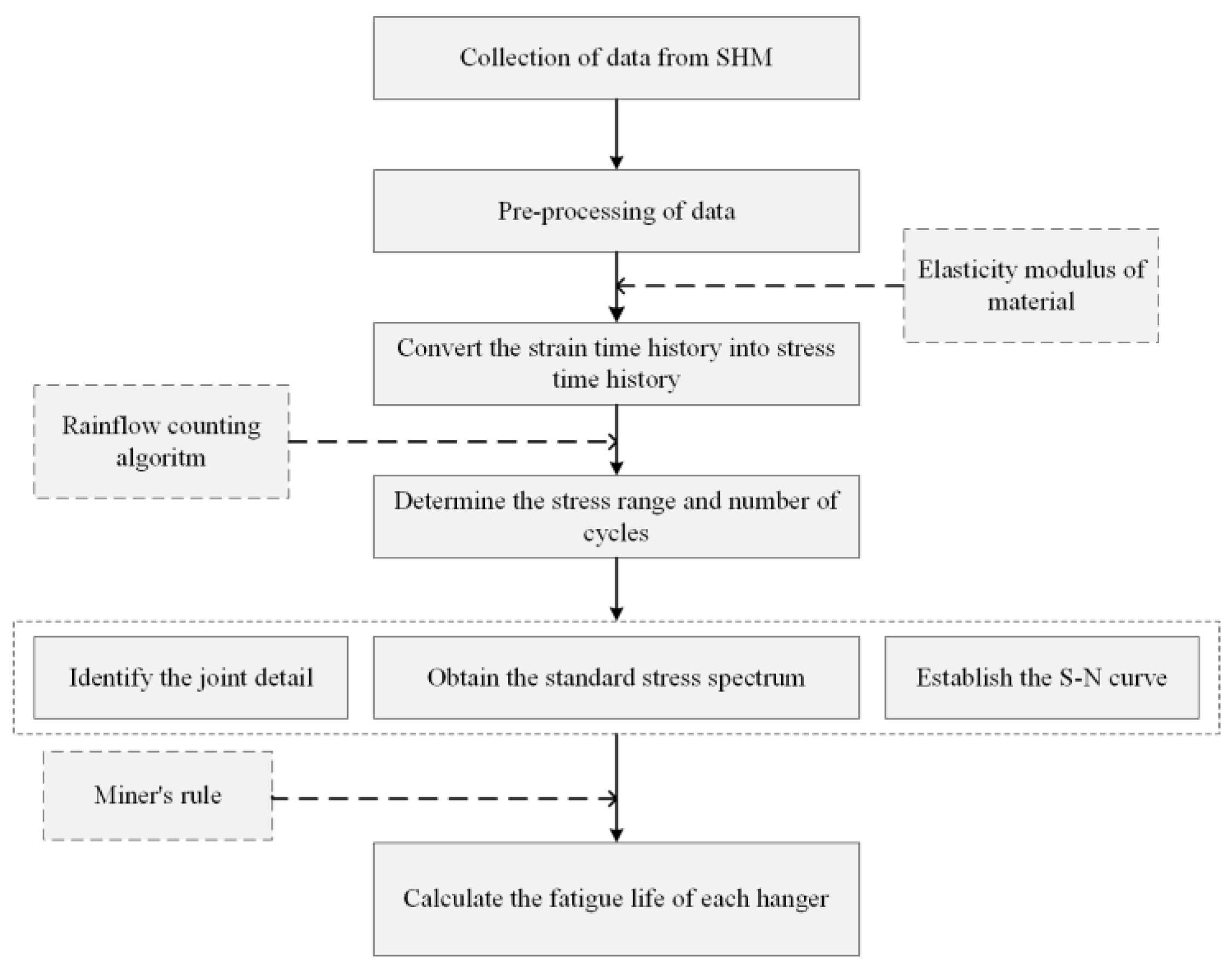
The time history of the stress range $\mathsf{\Delta }\sigma$ is essential for fatigue damage calculation. It is usually stable for railway arch bridges due to the prearranged train operation plan. However, the traffic flow in highway bridges is excessively random because of various vehicle types, vehicle weights, traveling speeds, etc. This is likely why few investigations have been conducted to assess the fatigue performance of hangers in highway arch bridges. In this study, a strain monitoring-based fatigue assessment method is proposed, as shown in the flowchart in Figure 1.

Using this approach, the time history of dynamic strain can be easily determined from a structural health monitoring (SHM) system. Noise disposal processing should be conducted to remove measurement noise for long-distance transmission and environmental interference. Then, the correlation stress series can be obtained by multiplying the strain by the elasticity modulus, since the steel material works within elastic strength range under normal traffic conditions. In application of the rain-flow counting algorithm, the stress range and number of cycles can be determined, and then the standard daily stress spectrum can be calculated by averaging a series of daily stress spectra in conditions of the traffic flow keeping relatively stable over 1 day. Then, the stress range is segmented from the standard daily stress spectrum and the S–N curve is established. Finally, the fatigue life of each hanger can be evaluated according to Miner’s rule, and three different codes are used for comparison in this study.

3. Field Measurement on Tian Yuan Bridge

3.1. Introduction of Tian Yuan Bridge

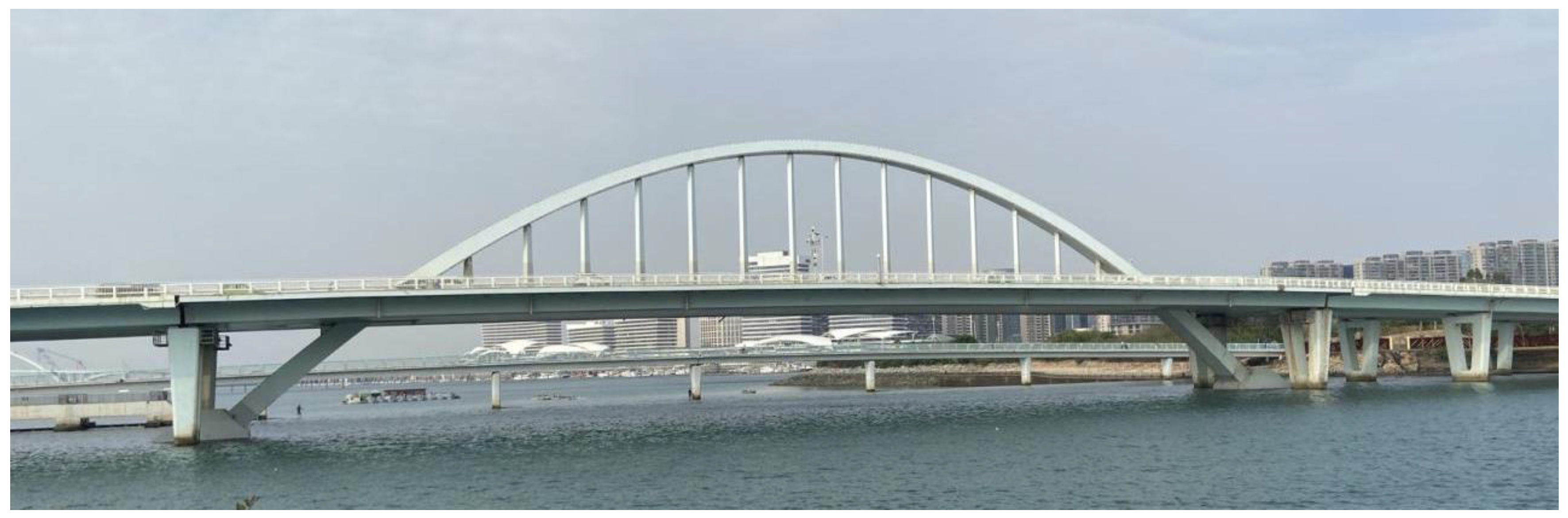
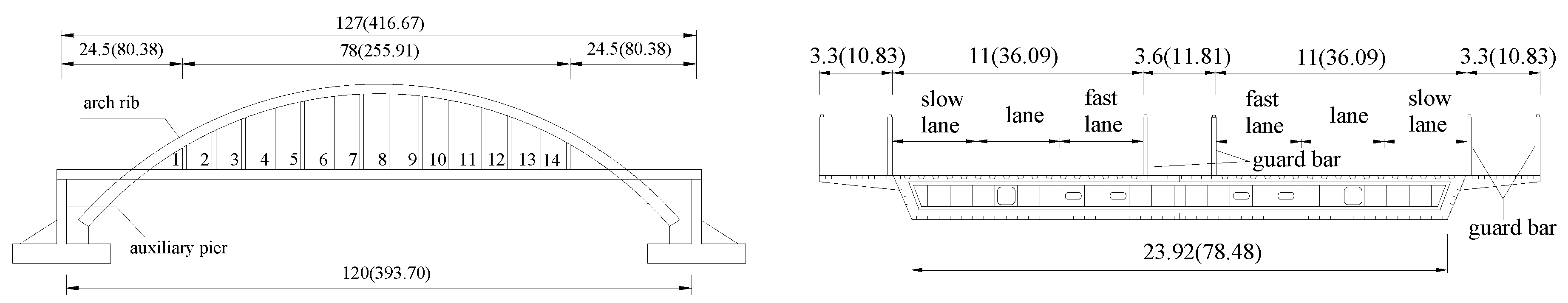
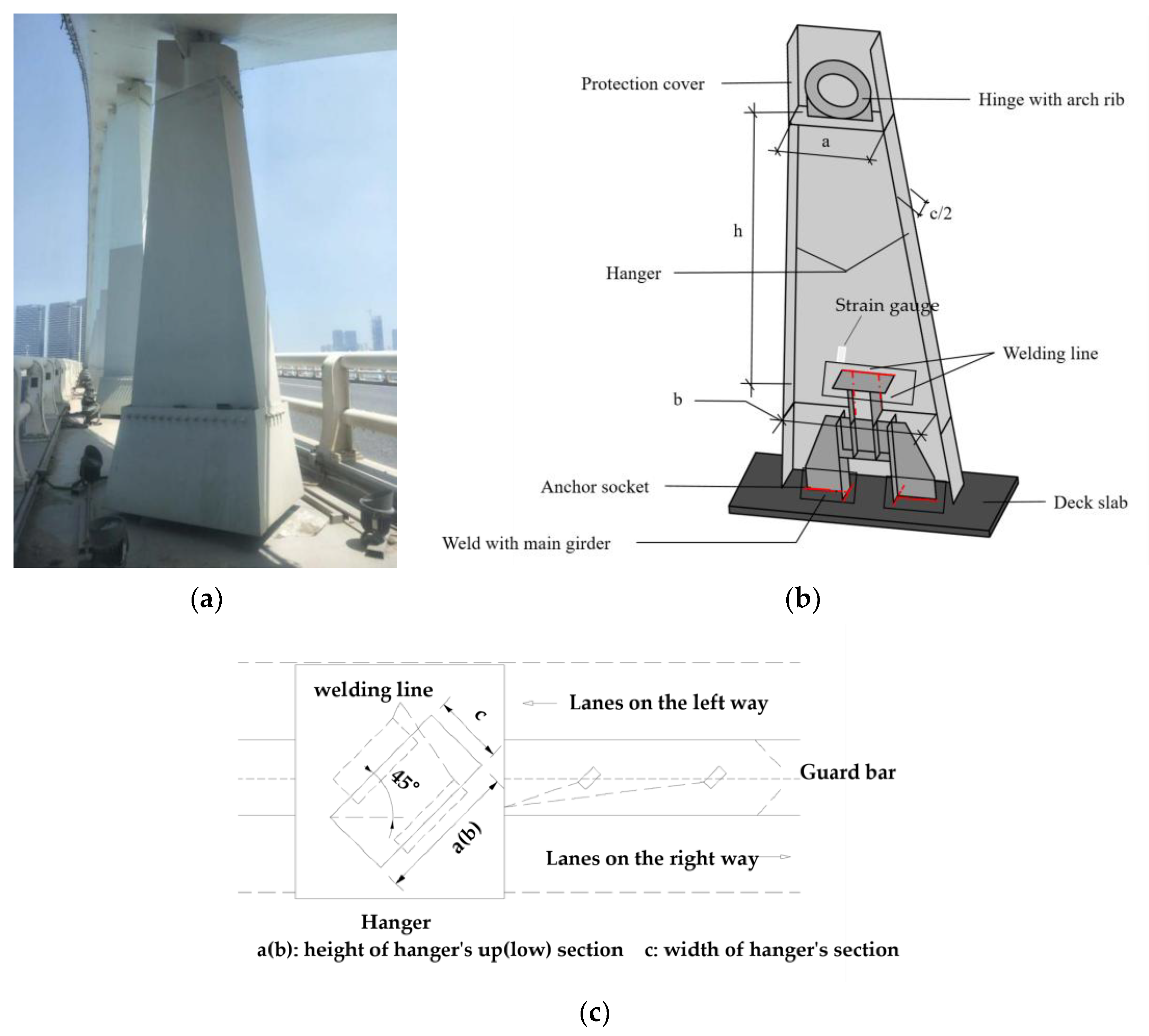
In this study, the Tian Yuan Bridge in Xiamen (China) was selected to demonstrate the application of the proposed method. As shown in Figure 2 and Figure 3, this steel arch bridge (open to traffic since 2007) has a span length of 127 m, in which the arch rib passes through the box girder. The deck slab is linked to the rib by 14 hangers with a longitudinal central spacing of 8 m. According to the plan, the horizontal angle between one primary symmetrical axis of the hanger’s section and the longitudinal axis of the girder is 45°. Six lanes are arranged in two directions on the bridge deck. The box-section hangers are formed by welding four pieces of 12 mm thick steel plates. Each hanger, as shown in Figure 4, is pin-connected to the arch rib at its upper end, and fixed to the deck plate through a special anchorage base at its lower end. The dimensions of the hangers are listed in

Table 1. Geometrical configuration of hangers.

Hanger ID	a (mm)	b (mm)	c (mm)	h (mm)
1	700	1219	476	2643
2	979	1208	476	6042
3	1049	1206	476	8878
4	1080	1205	476	11,156
5	1096	1204	476	12,872
6	1105	1204	476	14,026
7	1108	1204	476	14,621

. The steel material is Grade Q345-C as indicated in the design specification, with an elastic modulus specified as 205 GPa according to the code GB50017-2017.

3.2. Vehicle–Bridge Interaction (VBI) Model

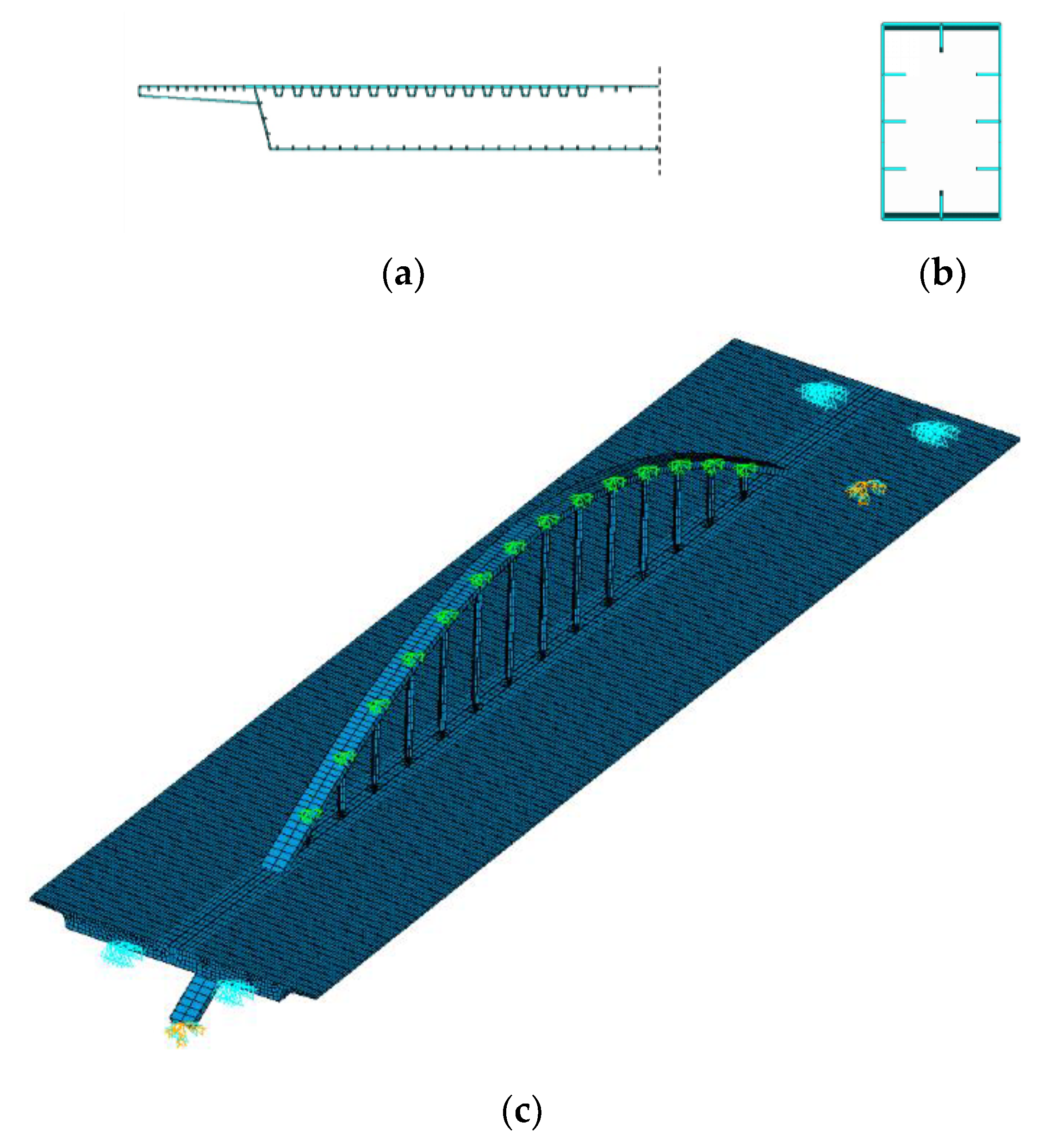
A numerical model of the VBI system was built in this study for stress analysis of the stiff hangers. An iterative procedure [19] was used to solve the interaction between the vehicle and bridge. The finite element (FE) model of the Tian Yuan Bridge adopted shell elements for the hangers and main box girder, and beam elements for the arch rib, as shown in Figure 5. The main girder and the hangers were simulated with the shell elements (six degrees of freedom (DOFs) at each node), and the arch rib was built with beam elements (six DOFs at each node). There were a total of 56,186 nodes and 61,312 elements in the bridge model. The box girder was simply supported while the arch rib was fixed. The lower end of the hanger was fixed to the anchorage base by tying its nodes to the welded line. The same connection was adopted between the anchorage base and deck slab. Since the upper end of the hanger was connected to the arch rib by a hinge, the connection condition in the FE model was simulated as a displacement constraint in both vertical and horizontal directions with the rib but free in rotation.

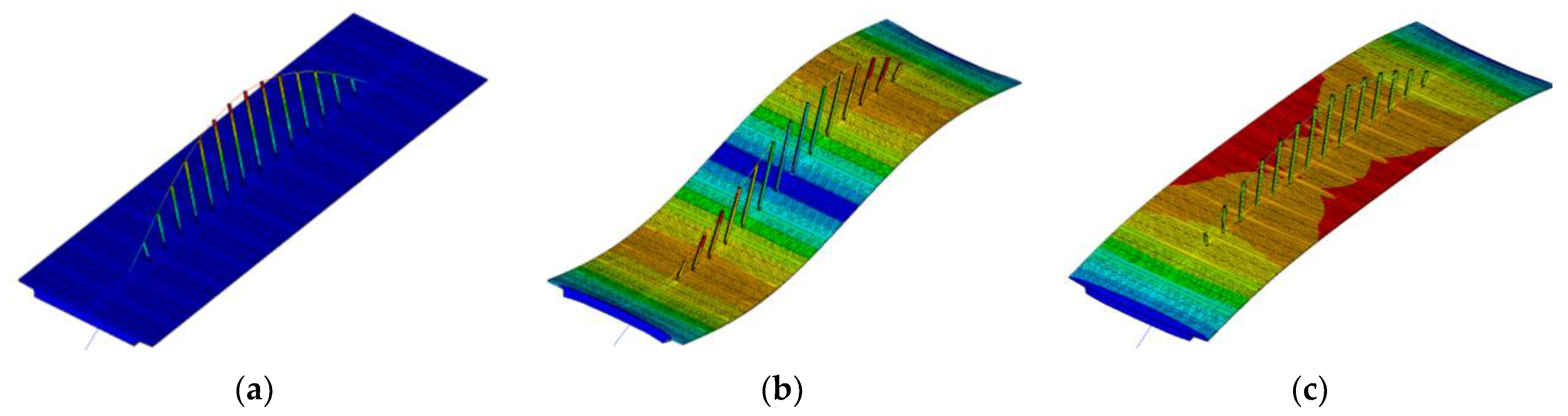
In the FE model, the first three frequencies of the bridge were 0.255 Hz, 1.007 Hz, and 1.525 Hz, while, in the field measurement, the first three frequencies were 0.244 Hz, 0.977 Hz, and 1.465 Hz. The first three mode shapes are shown in Figure 6.

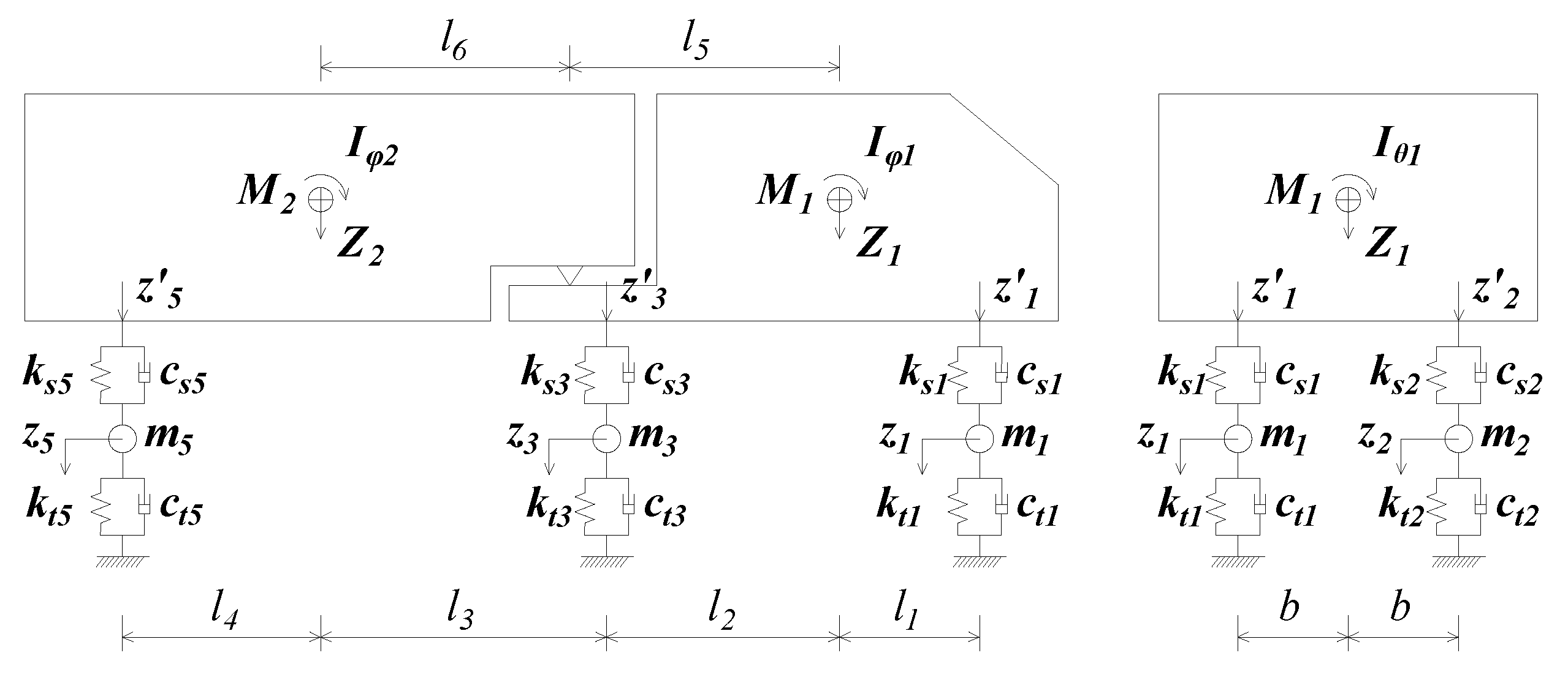
The FE model of an HS20-44 truck, which is frequently used in vehicle–bridge interaction systems according to AASHTO bridge design specifications, was also constructed (shown in Figure 7) in this study. It consisted of 11 independent DoFs [20]. The governing equation of the truck can be written as follows:

$$M_v{\ddot{Z}}_v+C_v{\dot{Z}}_v+K_v{Z}_v=G_v+F_{bv},$$

(1)

where $M_v$, $K_v$, and $C_v$ are the mass, stiffness, and damping matrices, ${\ddot{Z}}_v$, ${\stackrel{.}{Z}}_v$, and ${\stackrel{}{Z}}_v$ are the acceleration, velocity, and displacement, respectively, $F_{bv}$ is the instantaneous contact force at the points where the wheels contact the bridge, and $G_v$ is the gravity force.

The road profile is usually represented by a zero-mean stationary random process that can be expressed by a power spectral density (PSD) function. In this study, a modified PSD function [21] was used:

$$\varphi (n)=\varphi (n_0){\left(\frac{n}{n_0}\right)}^{-\omega }\hspace{1em}\hspace{1em}\hspace{1em}\hspace{1em}(n_1<n<n_2),$$

(2)

where $n$ is the spatial frequency (cycle/m), $n_0$ is the discontinuity frequency (0.5π cycles/m), $\varphi (n_0)$ is the roughness coefficient (m³/cycle), and $n_1$ and $n_2$ are the lower and upper cutoff frequencies, respectively. Then, the road surface roughness was determined in the space domain by applying the inverse Fourier transform.

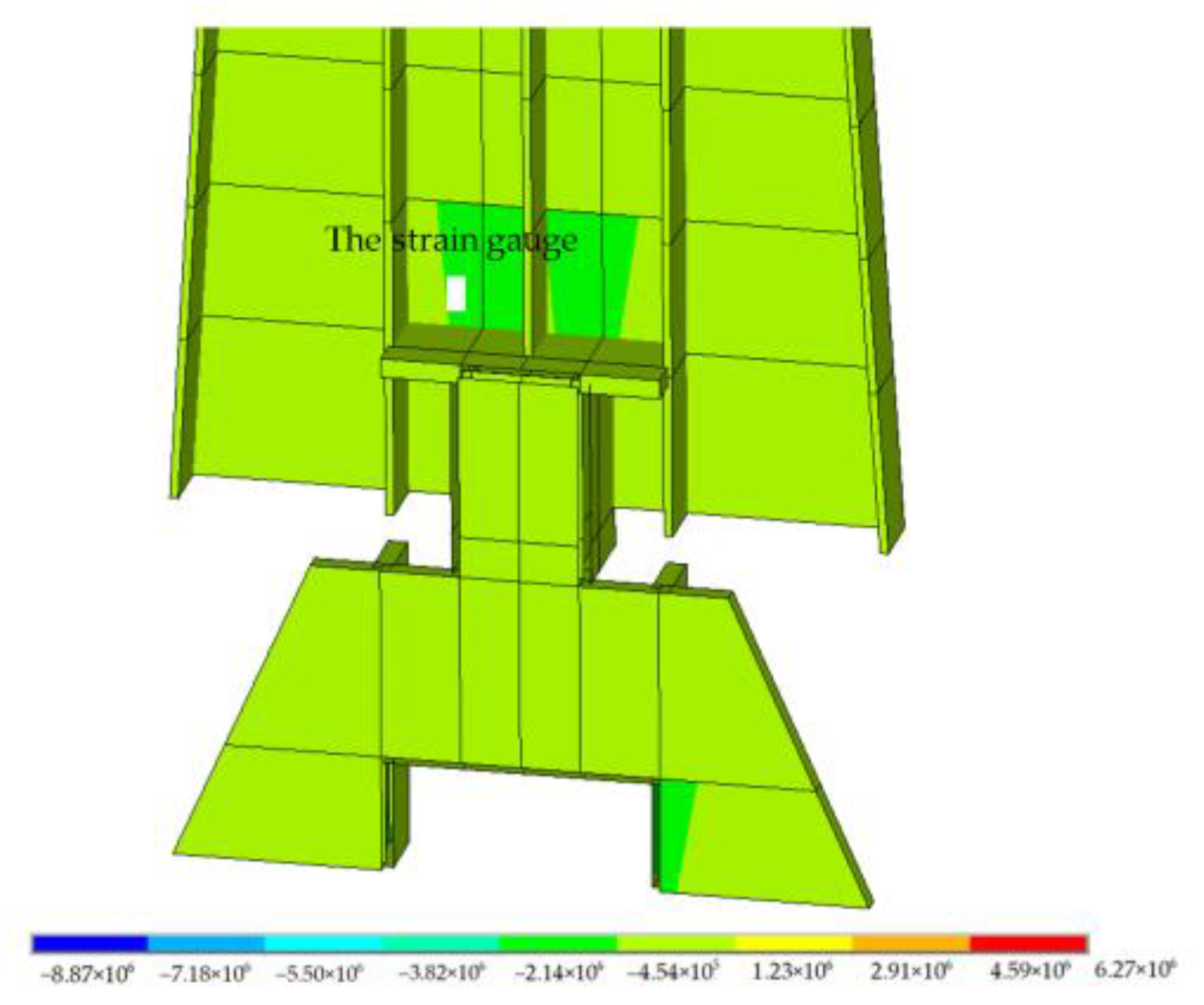
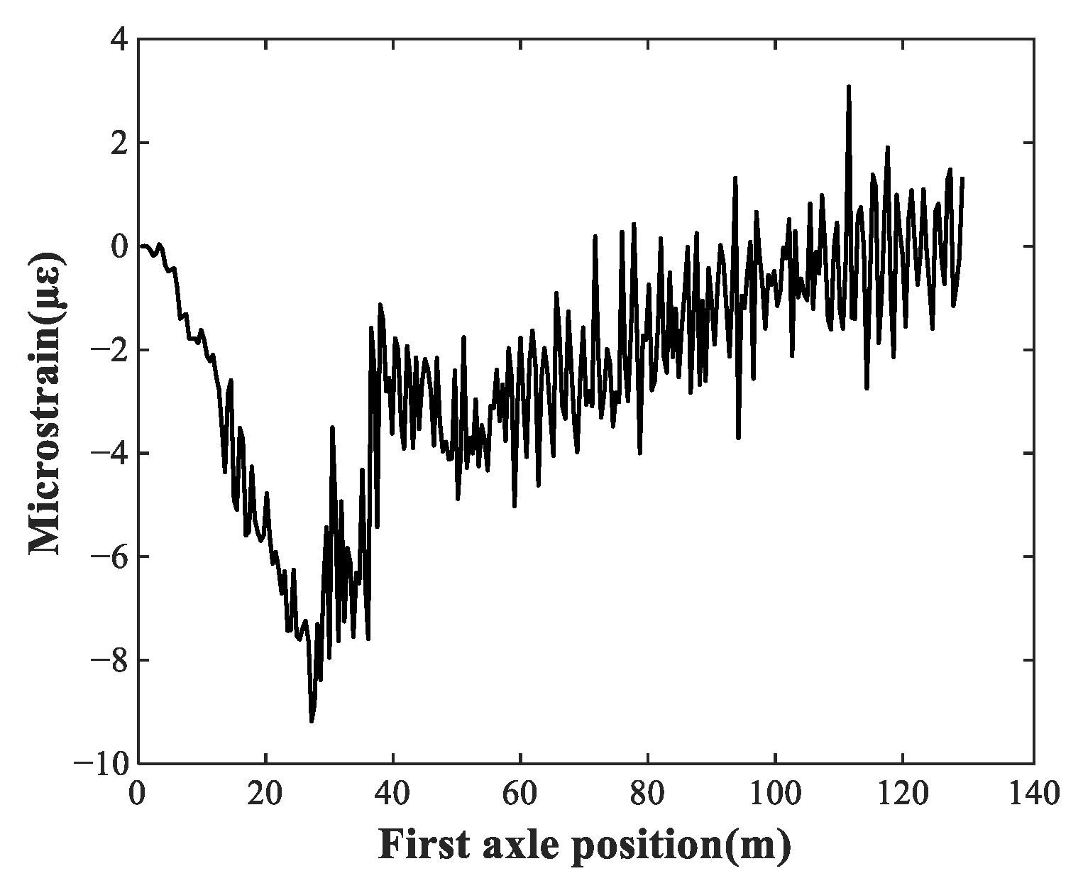
As investigated in a previous study [22], the bending effect is more significant at the hanger’s end zone close to an anchor base. To determine the potentially most dangerous location of strain gauge installation, an FE simulation of a HS20-44 truck traveling over the bridge with a velocity of 30 km/h in lane 3 was conducted, where the road surface condition was at an average level. Figure 8 shows the stress distribution in the connection area between the hanger slab and anchor socket; therefore, the strain gauge was placed near the end of key welding line. Figure 9 demonstrates the simulated strain response at the corresponding location on the first hanger.

3.3. Strain Measurement

The hangers labeled 1 to 7 in the left span were selected in the field measurement, and the strain data of the seven hangers were collected. All strain gauges were KFG series 119 Ω gauges with a 20 mm gauge length. Their longitudinal axes were placed parallel to the longitudinal axis of each hanger. All strain data were sampled continuously at a sampling frequency of 100 Hz, and 8.64 million data points were collected from each embedded gauge in 1 day. The empirical mode decomposition ($EMD$) algorithm for noise filtering was adopted in this study to preprocess the collected strain data. The most useful signal can be retained by removing the high-frequency components from the original signal [23,24,25].

To verify the applicability of the signal preprocessing method in this study, the time history of dynamic strain at the critical location in the first hanger was used, where the HS20-44 truck traveled over the bridge at 0.08 m/s in lane 3 in the VBI model. Gaussian white noise (4 dB, 7 dB, 10 dB, and 13 dB) was added to the signal to simulate the polluted signal in practice. A threshold, $k$, was used in the filtering, the order of the intrinsic mode function ($IMF$) less than $k$ was filtered, and the remaining $IM{F}_S$ were used to reconstruct the signal.

To evaluate the noise filtering effect under various conditions, the signal-to-noise ratio ($SNR$) improvement indicator $SNRI$ is defined as

$$SNRI=\frac{SN{R}_{\mathrm{out}}-SN{R}_{\mathrm{in}}}{SN{R}_{\mathrm{in}}}100\%,$$

(3)

and the $SNR$ is expressed as

$$SNR=10\lg \left(\frac{{\displaystyle \sum _{n=1}^N{s}^2(n)}}{{\displaystyle \sum _{n=1}^N{[s(n)-\overline{s}(n)]}^2}}\right)$$

(4)

where $s(n)$ is the noise-containing signal, $\overline{s}(n)$ is the noise-free signal, and $N$ is the number of sampling signals (unit: dB); $SN{R}_{\mathrm{in}}$ is the SNR of the signal input, while $SN{R}_{\mathrm{out}}$ is the $SNR$ of the signal output via $EMD$ algorithm filtering.

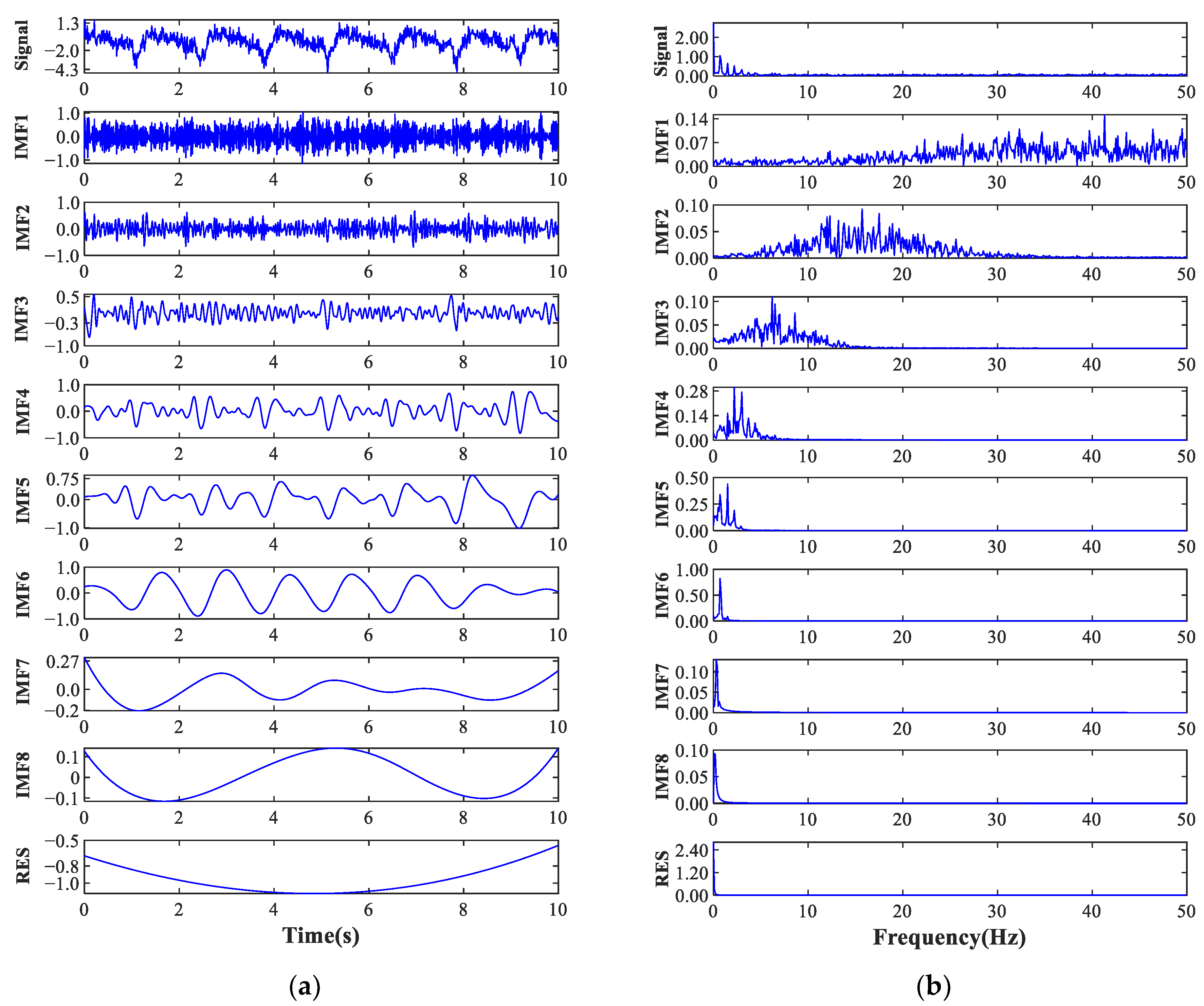
$SNRI$ is the relative increment in signal-to-noise ratio after preprocessing. By comparing the $SNRI$ with different thresholds, one can examine the optimal k to achieve the desired noise filtering effect. Figure 10 shows an example of applying the $EMD$ algorithm to the time history of the strain ($SNR=7 \mathrm{dB}$) obtained in the numerical simulation. As expected, the $IMF$ with higher order contained lower-frequency components. In order to find the most suitable threshold, k = 1, 2, 3, and 4 was used, and the results of $SNRI$ are listed in

Table 2. The SNRI with different SNR_in and IMF_k.

$\mathit{I}\mathit{M}{\mathit{F}}_{\mathit{k}}$ Threshold	SNRin (%)
	4 dB	7 dB	10 dB	13 dB
1	100.91	53.73	32.70	24.84
2	186.15	88.91	56.78	43.06
3	267.23	115.22	63.31	44.50
4	135.70	45.60	9.334	−11.52

. It is shown that the $EMD$ algorithm could achieve a great noise filtering effect when $SNR=4 \mathrm{dB}$, 7 dB, 10 dB, and 13 dB; in particular, the $SNRI$ reached the maximum value when the threshold was 3.

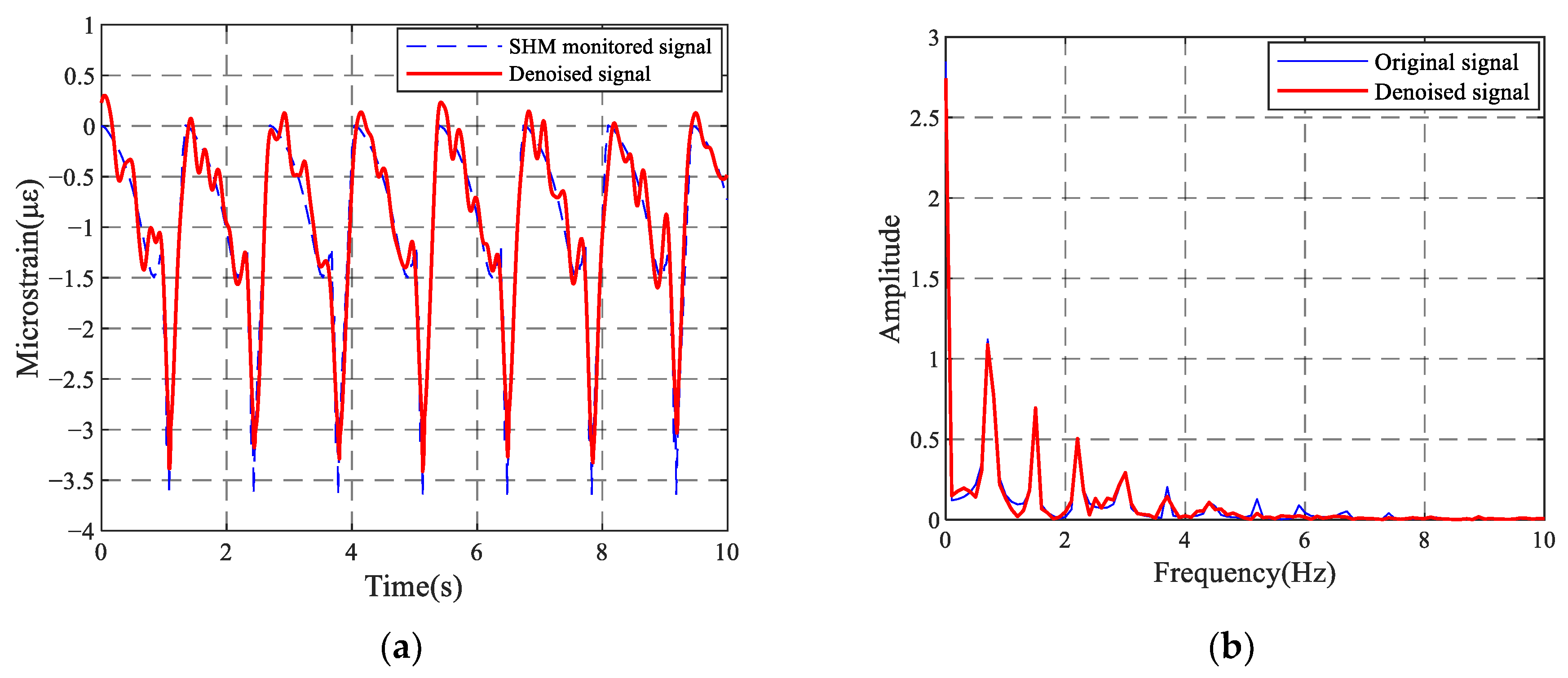
A comparison between the original signal and the filtered signal is shown in Figure 11. When the threshold was 3, most of the noise was removed, and the majority of useful information in the original signal could be retained, indicating that the $EMD$ algorithm is applicable to filter noise from the strain data of the Tian Yuan bridge model. Moreover, it can be seen in Figure 11b that the identified frequencies from the filtered signal matched well with those in the field measurement mentioned in Section 3.2.

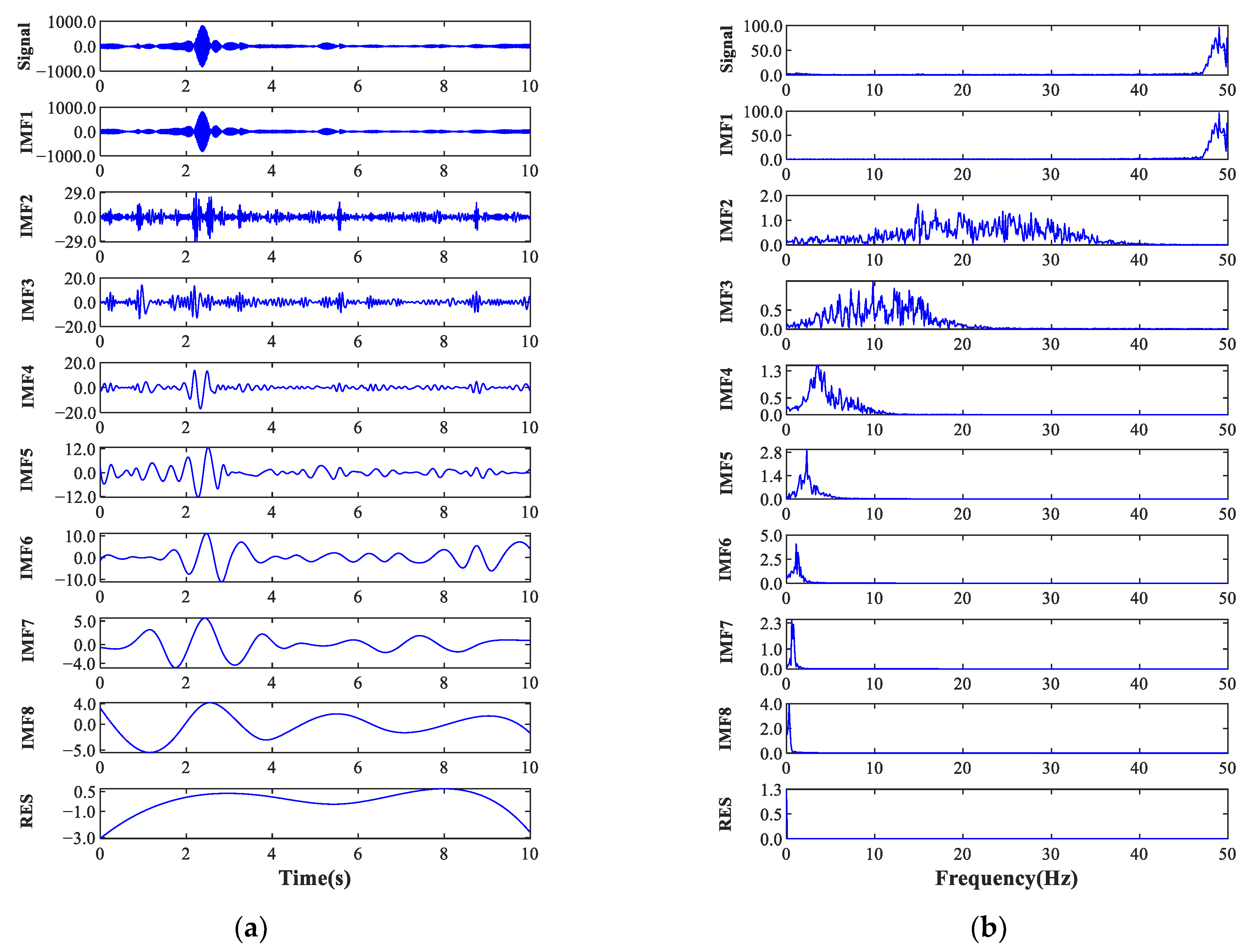
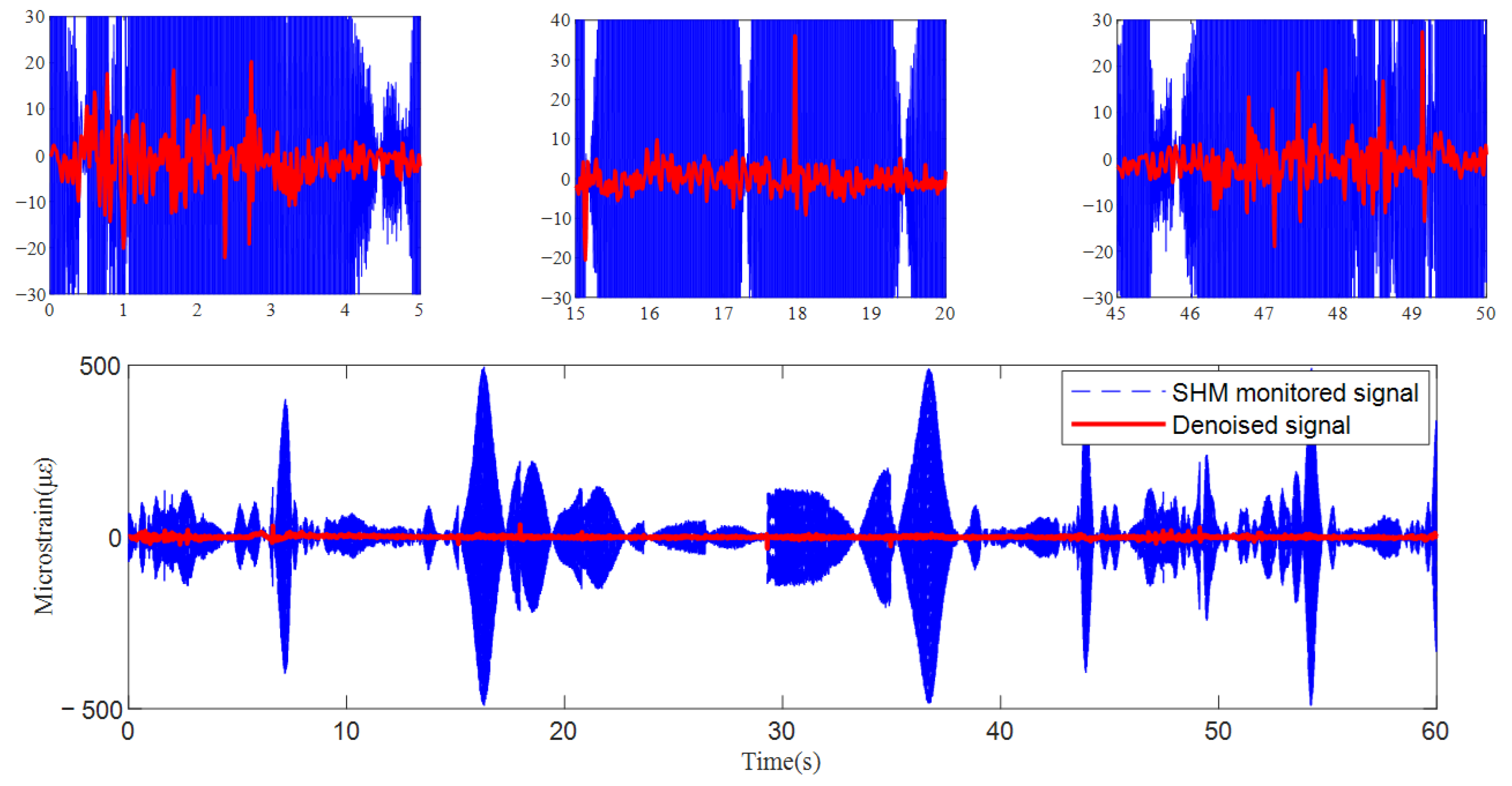
Figure 12 illustrates the application of the $EMD$ algorithm to the time history of field strain measurement from the first hanger. It is shown that the raw data were heavily polluted by noise. The spectrum of $IM{F}_1$ stood out sharply between 49 Hz to 50 Hz, indicating that the original signal received interference from the electrical noise with a frequency of 50 Hz. This component had much greater amplitude than the vibration component related to the bridge vibration. The spectrum of $IM{F}_2$ was a typical pattern of white noise, and the spectra of $IM{F}_3$ and $IM{F}_4$ were similar to those in Figure 10. The remainder was considered to be thermal-induced strain. Hence, a threshold of 3 was adopted to remove the noise and reconstruct the signal. As shown in Figure 13, the raw strain data collected from the monitoring system were seriously distorted; therefore, they could not be used directly. The $EMD$ algorithm worked quite well in filtering noise and obtaining the signal that could reflect the vibration behavior in the bridge.

4. Statistical Analysis of Stress Spectrum

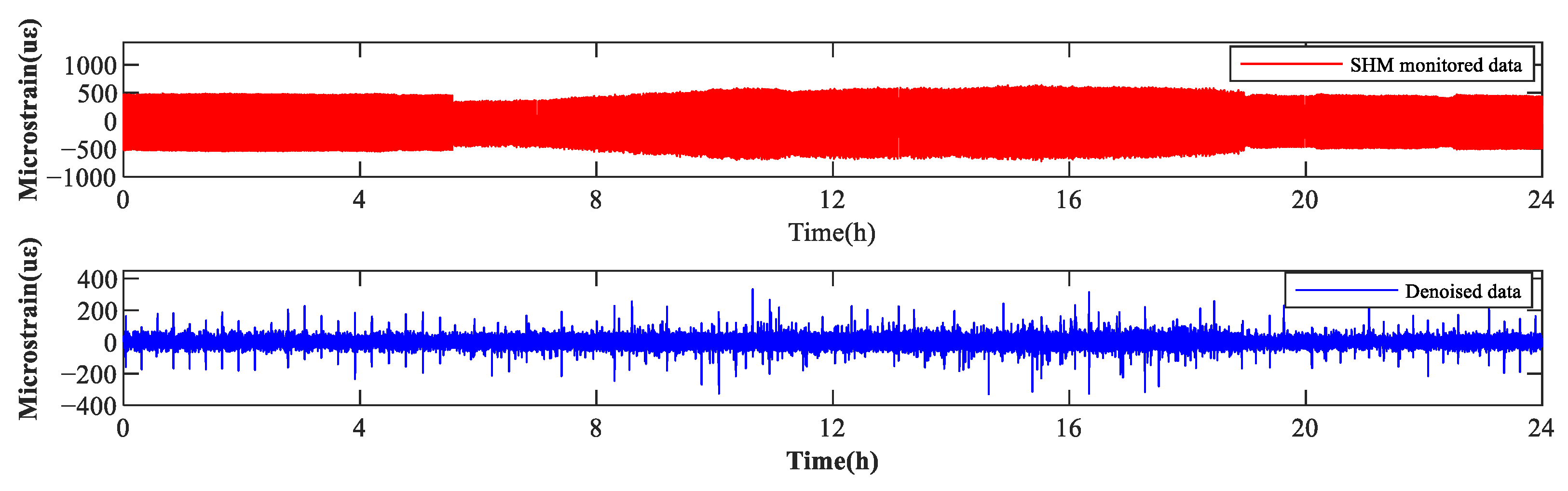
Although other loadings such as temperature, humidity, and wind were also applied to the bridge, Ye et al. [26] proposed that it was unnecessary to separate the strain response by different loadings since the count of stress range only depended on the deviation calculation between the peak and the valley in each stress cycle. As the sampling frequency was 100 Hz, a huge number of tiny stress pulses were formed in the strain histories. It is unreasonable to count very small pulses as individual stress cycles; thus, a stress cycle counting method should be used to remove the irregular pulses. The rain-flow counting algorithm [27] can separate small stress ranges from larger ones such that a number of continuous small variable stress can be eliminated. Therefore, the rain-flow counting algorithm was employed to improve computation efficiency. The strain data monitored in the period from July 2020 to June 2021 were selected in this study. The strain data were absent on a few days for reasons such as rust-preventing coating. Hence, the strain data were only collected on 159 days during this period. The duration of 1 day (24 h) was adopted as the time unit in the statistical analysis of stress cycles. All strain data were filtered using the EMD algorithm to first remove noise, as shown in Figure 14.

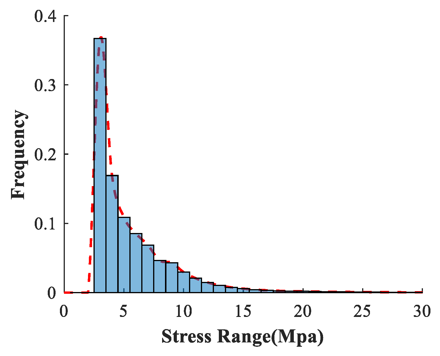
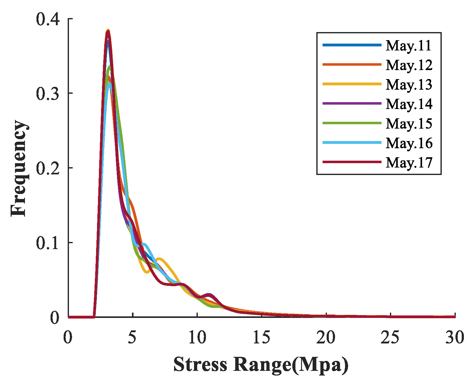
Subsequently, the statistical daily stress spectrum could be obtained by executing the rain-flow cycle counting technique. Figure 15 shows the histograms of typical daily stress spectra specifying a resolution of 1 MPa for the stress range interval in normal traffic conditions. The amplitudes less than 2 MPa are not shown for clarity. The daily stress spectra are represented by curves in Figure 16.

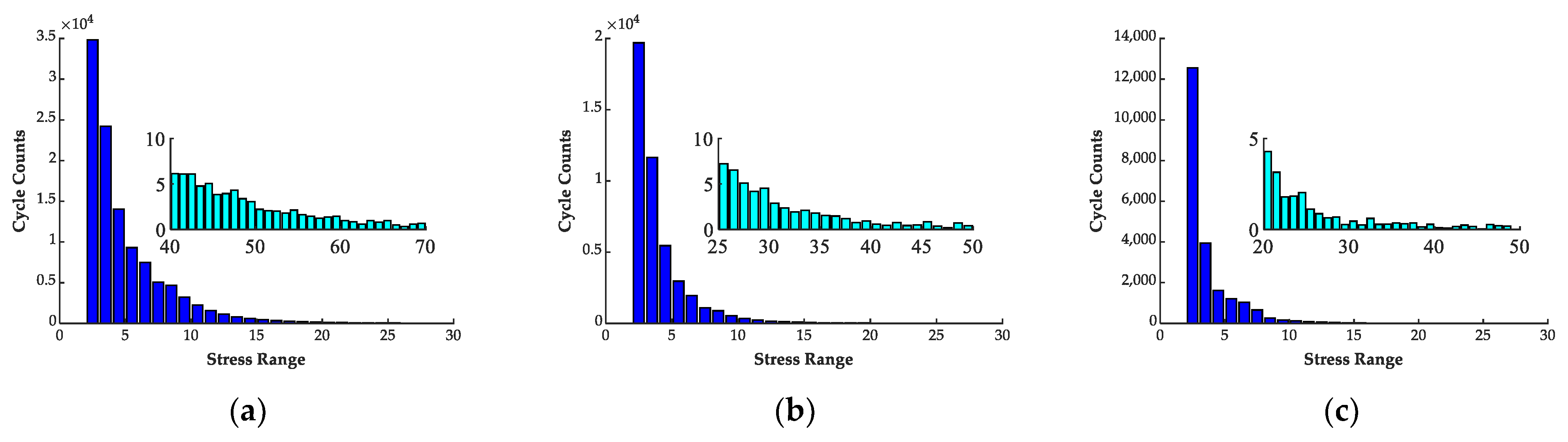
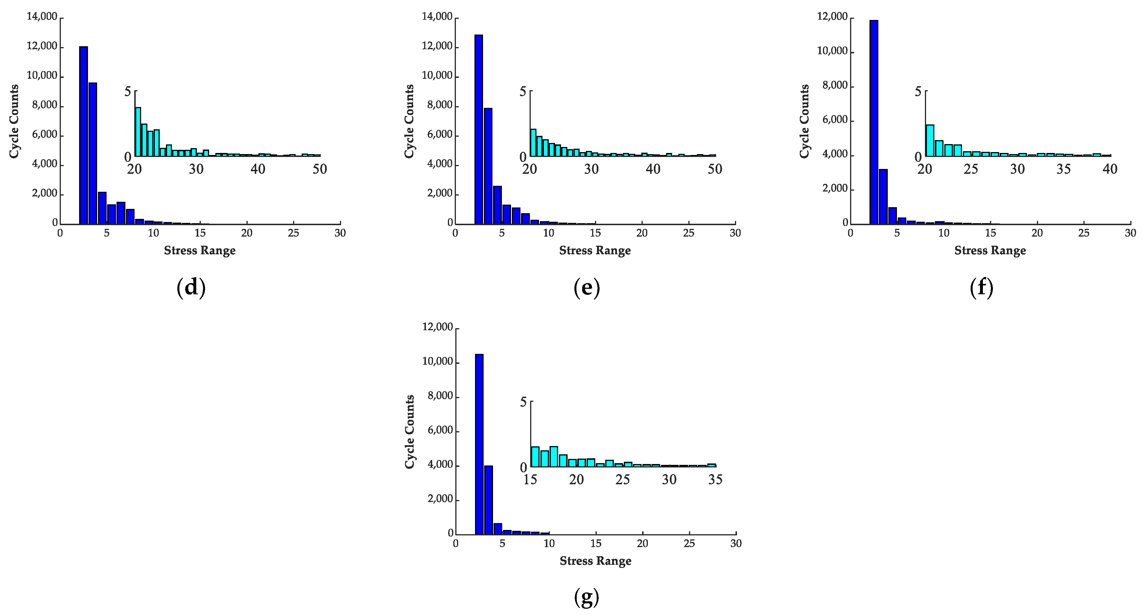
The standard daily stress spectrum which was obtained by averaging the 159 day stress is given in Figure 17. The range of the daily stress spectrum gradually decreased with the increase in hanger length. The shortest hanger (the first hanger) had a stress range of approximately 70 MPa, while the longest hanger (the seventh hanger) had a stress range within 30 MPa. More detailed statistics are available in

Table 3. Statistics of standard daily stress spectrum.

Hanger Number	Stress Range (MPa)
	0–2	2–10	11–20	21–30	31–40	41–50	51–60	61–70	71–80	81–90	91–100
1	1,525,030	92,152.0	7861.8	672.5	151.6	46.8	17.4	7.3	3.2	2.2	1.3
2	1,641,476	44,229.2	1142.8	99.0	17.0	5.2	2.7	1.3	1.3	1.0	0.4
3	1,731,491	21,476.0	399.7	16.7	3.3	1.4	0.9	0.4	0.4	0.3	0.2
4	1,722,854	28,229.3	504.2	13.6	1.9	1.2	0.6	0.2	0.2	0.2	0.1
5	1,655,334	26,888.2	403.6	9.1	1.8	1.0	0.7	0.3	0.2	0.1	0.1
6	1,657,919	13,131.8	27.6	2.3	0.4	0.2	0.1	0.1	0.0	0.1	0.0
7	1,684,762	16,863.7	129.6	2.4	0.3	0.2	0.1	0.1	0.0	0.0	0.0

.

5. Fatigue Assessment

5.1. According to the Chinese Code for Design of Steel Structures

Part 16 of the Chinese Code for Design of Steel Structures (GB50017-2017) is commonly used in fatigue damage calculation and life assessment for steel structures in China, according to the allowable stress range methodology and fatigue damage cumulative theory. The variable stress range fatigue problem can be converted into an equivalent constant stress range fatigue problem. When the general equivalent stress range $\Delta \sigma$ satisfies Equation (5), a structural component or connection is considered as reaching its critical fatigue safety state.

$$\{{}_{\Delta \sigma ={(({[\Delta \sigma ]}_{5\times {10}^6})\frac{Cz}{n})}^{\frac{1}{{\beta }_{z+2}}},\hspace{1em}\hspace{1em}5\times {10}^6<n<1\times {10}^8}^{\Delta \sigma ={(\frac{Cz}{n})}^{\frac{1}{{\beta }_z}},\hspace{1em}\hspace{1em}n<5\times {10}^6},$$

(5)

where $C_z$ and ${\beta }_z$ are determined according to GB50017-2017 as $C_z=2\times {10}^{12}$ and ${\beta }_z=3$; ${[\Delta \sigma ]}_{5\times {10}^6}$ is the allowable fatigue stress range when the number of fatigue stress cycles $n_{}$ reaches $5\times {10}^6$, which is determined according to the GB50017-2017 as 74 MPa.

According to the Palmgren–Miner linear damage accumulation theory, the fatigue damage accumulation index $D$ is expressed as

$$D={\displaystyle \sum \frac{n_i({\sigma }_i){\beta }_z}{C_z}}+{\displaystyle \sum \frac{n_j({\sigma }_j){\beta }_z}{{C_z}^{\prime }}},$$

(6)

$${C_z}^{\prime }={(\Delta {\sigma }_{5\times {10}^{{}^6}})}^2{C}_z,$$

(7)

where $n_i$ is the stress cycle number when the stress range $\Delta {\sigma }_i$ satisfies $\Delta {\sigma }_{[5\times {10}^6]}<\Delta {\sigma }_i$, and $n_j$ is the stress cycle number when $\Delta {\sigma }_L<\Delta {\sigma }_j\le \Delta {\sigma }_{[5\times {10}^6]}$. This means that the structural component or connection may reach fatigue failure when $D=1$. After obtaining the standard daily stress spectra, the fatigue life of the connection can be evaluated accordingly. For a variable stress range, $\Delta {\sigma }_{eq}$ can be obtained as

$$\Delta {\sigma }_e{}_q={\left[\frac{{\displaystyle \sum n_i{(\Delta {\sigma }_i)}^{{\beta }_z}}+{\left({[\Delta \sigma ]}_{5\times {10}^6}\right)}^{-2}{\displaystyle \sum n_j{(\Delta {\sigma }_j)}^{{\beta }_z+2}}}{2\times {10}^6}\right]}^{1/{\beta }_z},$$

(8)

where the equivalent number cycles of $\Delta {\sigma }_{eq}$ is $2\times {10}^6$. Thus, the fatigue life of the structural component, which is normally represented in terms of the number of years, can be calculated as

$$Y=\frac{C_Z}{365\times 2\times {10}^6\times \Delta {\sigma }_{eq}{}^{{\beta }_z}}.$$

(9)

5.2. According to Eurocode 3

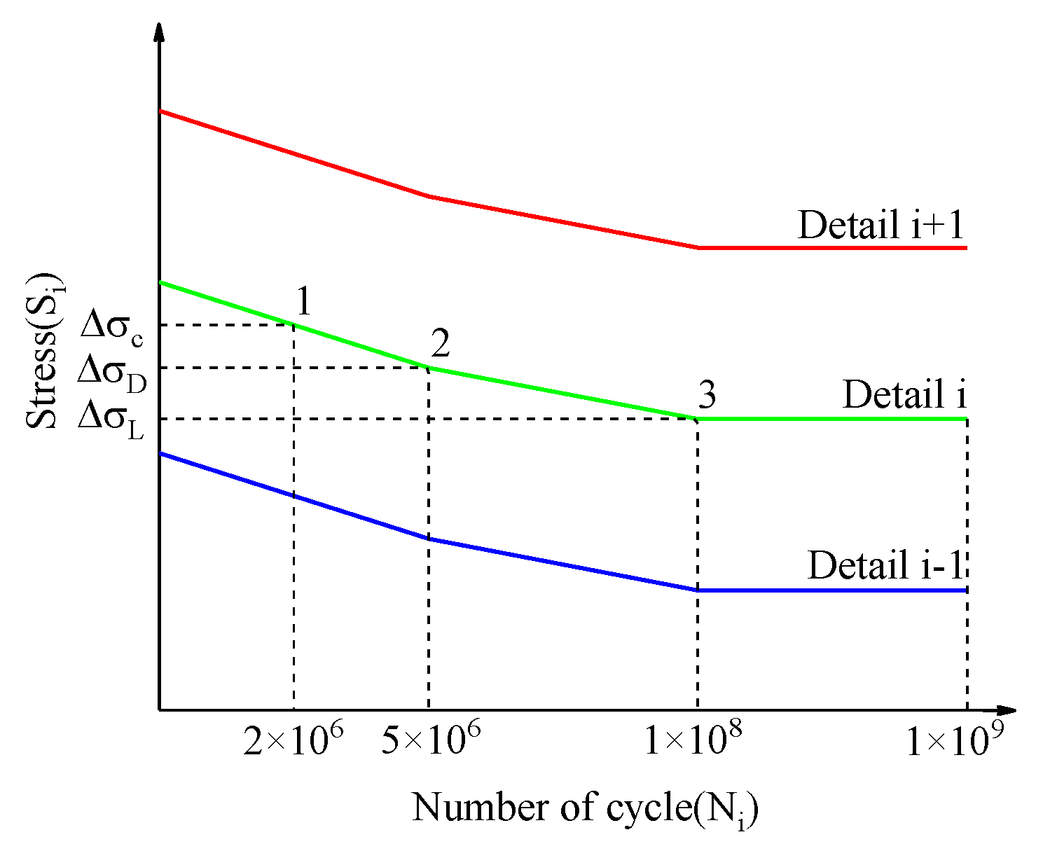
The S–N curve, obtained from the experimental results for different materials and different categories of welded details, was applied to calculate the cumulative fatigue damage of structural components. Each S–N curve provided in Eurocode 3 is composed of two oblique line segments and a horizontal one. For different detail categories, the curves satisfy a parallel relationship.

As shown in Figure 18, the slope of the first line segment from point 1 to point 2 was equal to 3, while that of the second segment from point 2 to point 3 was equal to 5. $\Delta {\sigma }_C$ is the stress range level when the number of fatigue stress cycles $N_i$ reaches $2\times {10}^6$. $\Delta {\sigma }_D$ is the constant-amplitude fatigue limit, or the stress range level when $N_i$ reaches $5\times {10}^6$. $\Delta {\sigma }_L$ is the cutoff stress range limit value, or the stress range level when $N_i$ reaches $1\times {10}^8$. No fatigue damage is expected to happen when $\Delta {\sigma }_i<\Delta {\sigma }_L$, according to the stipulation in this code.

The structural component fatigue life, which is expressed as the number of stress cycles $N_i$ under various stress levels, is supposed to satisfy the following equation:

$$\Delta {\sigma }_i{}^k\cdot N_i=\{{}_{K_D=\Delta {\sigma }_D{}^5\cdot 5\times {10}^6,\hspace{1em}\hspace{1em}5\times {10}^6<N_i\le {10}^8}^{K_C=\Delta {\sigma }_C{}^3\cdot 2\times {10}^6,\hspace{1em}\hspace{1em}{N}_i\le 5\times {10}^6},$$

(10)

where $k$ is the reciprocal of the slope of an oblique line segment, and $K_C$ and $K_D$ are coefficients of S–N curve. The coefficients are determined according to Eurocode 3 as $K_C=2\times {10}^{12}$, $K_D=1.08719\times {10}^{16}$, $\Delta {\sigma }_C=100 \mathrm{MPa}$, $\Delta {\sigma }_D=73.7 \mathrm{MPa}$, and $\Delta {\sigma }_L=40.4613 \mathrm{MPa}$ when the weld joint is categorized as detail 100, which can be used in the subsequent calculation of fatigue life.

The fatigue damage index $D$ in cases of stress with variable amplitude can be expressed as

$$D={\displaystyle \sum _{}\frac{n_i\cdot \Delta {\sigma }_i{}^3}{K_C}}+{\displaystyle \sum _{}\frac{n_j\cdot \Delta {\sigma }_i{}^5}{K_D}},$$

(11)

where $n_i$ is the stress cycle number when the stress range $\Delta {\sigma }_i$ satisfies $\Delta {\sigma }_D<\Delta {\sigma }_i$, and $n_j$ is the stress cycle number when $\Delta {\sigma }_L<\Delta {\sigma }_j\le \Delta {\sigma }_D$. The total repeated stress cycles during the whole fatigue load-bearing duration $N_d$ can be calculated as follows:

$$N_d={\displaystyle \sum _{\Delta {\sigma }_D\le \Delta {\sigma }_i\le \Delta {\sigma }_C}{n}_i+}{\displaystyle \sum _{\Delta {\sigma }_L\le \Delta {\sigma }_j<\Delta {\sigma }_D}{n}_j}.$$

(12)

According to the equivalent principle of fatigue damage, the variable-amplitude stress cycle is equivalent to a constant-amplitude stress cycle, and the equivalent stress range $S_{eq}$ is expressed as

$$S_{eq}={[\frac{{\displaystyle \sum _{\Delta {\sigma }_i>\Delta {\sigma }_{{}_D}}(n_i\cdot \Delta {\sigma }_i{}^3)/K_c+{\displaystyle \sum _{\Delta {\sigma }_L<\Delta {\sigma }_j\le \Delta {\sigma }_{{}_D}}(n_j\cdot \Delta {\sigma }_j{}^5)/K_D}}}{N_{\mathrm{d}}/K_D}]}^{1/5}.$$

(13)

Herein, the fatigue damage accumulation index $D$ is rewritten as

$$D=\frac{N_d\cdot {\mathrm{S}}_{eq}{}^5}{K_D}.$$

(14)

Obviously, fatigue failure of a structural component happens when $D=1$. On the basis of the daily monitoring of repeated dynamic stresses, the corresponding daily cycle number $N_d$ and equivalent stress range $S_{eq}$ can be calculated from Equations (12) and (13), respectively. Thus, the fatigue life in terms of the number of years can be presented as

$$Y=\frac{K_D}{365\cdot N_d\cdot {\mathrm{S}}_{eq}{}^5}.$$

(15)

5.3. According to AASHTO

The fatigue assessment of structural components in the AASHTO specifications is based on the same experimental data that correlate the magnitude of stress range ($S_i$) with the number of cycles to fatigue failure ($N$) for various types of detail:

$$N=A{S}_i{}^{-3},$$

(16)

where N is number of stress cycles to fatigue failure, $S_i$ is nominal stress range at a fatigue detail, and A is the detail category constant.

Since the S–N curve was developed primarily under constant-amplitude cyclic loading, the actual variable-amplitude cyclic loading on the structural components in the bridge can be equivalently expressed with an effective stress range:

$$S_{re}={({\displaystyle \sum {\gamma }_i{S}_{ri}{}^3})}^{1/3},$$

(17)

where $S_{re}$ is effective stress range of a variable-amplitude stress range histogram, $S_{ri}$ is the $i_{th}$ stress range in the stress range histogram, ${\gamma }_i=n_i/N$ is the ratio of occurrence of stress range $S_{ri}$ in the histogram, $n_i$ is number of occurrences of stress range $S_{ri}$, and $N$ is the total number of occurrences of all stress cycles in the histogram. That is, all stress ranges lower than $0.5CAFL$ are excluded in the calculation of effective stress range $S_{re}$. According to AASHTO specifications, $A=20.0\times {10}^{11} {\mathrm{MPa}}^3$ and $CAFL=82.75 \mathrm{MPa}$ when the weld joint is categorized as detail $B^{\prime }$.

According to the fatigue damage cumulative theory, the daily damage $D_i$ attributed to $S_{ri}$ is denoted as $D_i=n_i/N_i$ and $N_i=A/s_i{}^3$; thus, the total daily damage is $D={\displaystyle \sum D_i}=(N\times S_{re}{}^3)/A$. The structural fatigue failure happens when $D=1$. Thus, the fatigue assessment life is calculated as

$$Y=\frac{A}{365\times N\times S_{re}{}^3}.$$

(18)

5.4. Consideration of the Growth of Traffic Volume

With the noticeable annual growth of traffic volume, the bridge will suffer a growing amount of vehicle load; hence, the variation trend of the fatigue life should be considered. This increasing traffic flow leads to a continuous increase in the fatigue load effect on the bridge structure. Deng et al. [28,29] demonstrated that the traffic flow, except for some of occasional emergencies, would not exhibit unlimited nonlinear growth. Thus, a linearly increasing model was adopted to calculate the stress cycle times in the duration of the serving life. The cumulative number of stress cycles $N_t$ of structural component during the service period of $Y$ years can be written as

$$N_t=365\cdot N_d\cdot Y\cdot \left(1+\frac{\left(Y-1\right)\alpha }{2}\right),$$

(19)

where $\alpha$ is the vehicle load growth coefficient. According to the number of vehicles recorded by the Statistical Yearbook in Xiamen from 2005 to 2020, it is reasonable to take $\alpha$ as 2% (medium term) and 5% (long term). The updated fatigue cumulative damage index $D$ by Eurocode 3 is rewritten as

$$D=\frac{N_t\cdot S_{eq}{}^5}{K_D}=365\cdot N_d\cdot Y\cdot \left(1+\frac{\left(Y-1\right)\alpha }{2}\right)\frac{S_{eq}{}^5}{K_D}.$$

(20)

The welded detail of the structural component reaches its fatigue life $Y$ (years) when $D=1$; then, $Y$ can be calculated accordingly. The same computation process can be carried out according to Equations (9) and (18) derived using the calculation methods from Code GB50017-2017 and AASHTO.

5.5. Assessment Results

In the Tian Yuan Bridge, each hanger acts as spring support to the main girder. A large proportion of vehicle loads applied on the slab deck are transferred to the arch rib by all hangers. Hence, the safety of hangers is vital for the whole bridge. To reduce the heavy statistical workload of huge stress cycles, the low-value cycles in which the stress range is below 2 MPa are neglected in the fatigue life assessment method [26].

Table 4. Estimated fatigue life of tested hangers (in years).

Hanger Number	GB50017-2017			Eurocode 3			AASHTO
	0%	2%	5%	0%	2%	5%	0%	2%	5%
1	669	212	145	657	211	143	447	167	115
2	2525	455	298	2505	453	297	2006	401	264
3	7566	821	531	7531	819	529	6157	736	477
4	14,094	1138	731	13,922	1131	724	10,856	993	639
5	13,677	1121	720	13,559	1115	717	10,523	977	629
6	55,197	2299	1466	55,018	2296	1464	44,400	2058	1313
7	77,840	2740	1745	76,200	2711	1726	62,348	2447	1559

lists the estimated fatigue life. All tested hangers satisfy the fatigue safety criterion in the bridge’s designed life expectancy (100 years). However, the vehicle load growth significantly decreases the remaining life even if a small increase rate (2% or 5%) is considered. Thus, bridge maintenance is strongly advised to focus on the growth of traffic volume, and updating the fatigue assessment of the hangers is mandatory in the future service period.

Special attention should be paid to the shortest hanger. When the traffic volume growth is not considered, the estimated remaining life of the first hanger is 669 years, 657 years, and 447 years. This is much less than that of the longest hanger, the seventh hanger. The observation herein agrees with the previous study [30] that a shorter hanger generally suffers a more severe risk of fatigue damage.

In addition, it can be seen that the fatigue assessment results by the three codes were quite different. The calculated values of fatigue life by Eurocode 3 were close to those obtained by Chinese code GB50017-2017, because both codes use trilinear S–N curves with the same slope. However, AASHTO uses a bilinear S–N curve, which results in larger fatigue damage because all stress amplitudes have the same effect on cumulative damage.

BS5400 [31] states that high-stress amplitude will enlarge the initial defects of the components, resulting in a lower cutoff stress range. However, the stress amplitude below the cutoff stress range will also contribute to the accumulation of damage as time grows. In order to evaluate the fatigue life of components more safely and comprehensively, the influence of low stress amplitude on the fatigue life assessment is also discussed in this study.

Table 5. Effect of low stress on fatigue life on the first hanger.

Code	$\left[\mathit{\sigma }\right]\ge {[\mathit{\sigma }]}_{\mathit{L}}$			$[\mathit{\sigma }]\ge 0.5{[\mathit{\sigma }]}_{\mathit{L}}$			${[\mathit{\sigma }]}_{\mathit{L}}=0$
	0%	2%	5%	0%	2%	5%	0%	2%	5%
GB50017-2017	669	212	145	512	182	125	474	173	119
Eurocode 3	657	211	143	509	181	124	472	173	119
AASHTO	447	167	115	203	101	72	91	58	44

lists the estimated results in the first hanger when the effect of low stress range is considered. As can be seen, the variation of fatigue life calculated according to AASHTO is obvious, and the fatigue life decreases from 447 years to 91 years. The reason is that the main component of the total damage turns from high-stress amplitude at low frequencies to low-stress amplitude at high frequencies according to AASHTO when the effect of low stress amplitude is considered. Comparatively, GB50017-2017 and Eurocode 3 use trilinear S–N curves, and the main components of the total damage are still dominated by high stress amplitudes with low cycle counts. There is a significant reduction in fatigue life under the influence of both increasing traffic load and low stress range. Correspondingly, it is necessary to consider the growth of traffic and the effect of low stress range when assessing the life of bridge components.

6. Conclusions

A strain monitoring-based fatigue life assessment of the stiff hangers in the operational arch bridge with the regular serving condition was proposed in this study, and the measured data in a period of 159 days were used to validate the feasibility of this presented approach. An FE model of the VBI system was constructed, on the basis of which the measurement location in the stiff hangers could be determined. Then, a statistical analysis was carried out, and different daily stress spectra were derived using the rain-flow counting technique to calculate the stress range and respective occurrence frequencies over a time interval of 24 h. The estimated fatigue life of seven typical hangers was calculated using the average daily stress spectra. Subsequently, the different estimated results according to Chinese code GB50017-2017, Eurocode 3, and AASHTO were comparatively analyzed. The influence of noticeable annual growth in traffic volume and low stress range on the fatigue life was also discussed. The following conclusions could be drawn:

(i)

The bending effect at the end zone of the hanger induces uneven axial stress in the key connecting weld lines. Simulation calculations have great significance in determining the monitoring location in stiff hangers. The EMD technique is applicable in the preprocessing of extensive SHM data.

(ii)

In average traffic service conditions, each involved hanger showed steady dynamic behavior during a continuous measuring duration of 159 days. The shortest hanger showed comparatively higher stress ranges in the statistical histogram.

(iii)

According to the estimated results based on three reference codes, the stipulation in AASHTO formulated a relatively higher cutoff stress range than the other two codes. Therefore, its calculated fatigue life was shorter. The fatigue damage assessed referring to GB50017-2017 and Eurocode 3 had a similar calculation progress since the S–N curves were different. When the contribution of low-stress amplitude to fatigue damage was considered, the fatigue life was significantly reduced when using AASHTO specifications. Moreover, the annual traffic load growth had a great influence on prospective fatigue life.

(iv)

Comparing the estimated fatigue life of all measured hangers, it was verified that the shortest hanger showed more severe fatigue damage than longer hangers. This is consistent with [30], which showed that the shortest hanger transferred relatively complicated stress as it was adjacent to the area where arch rib went through the girder to its skewback. Additionally, it suffered a more distinct dynamic effect as it was closer to the expansion joint compared with other hangers. However, the intrinsic reason for the difference between longer hangers is worthy of further research and investigation.

References

- Xu, J.; Chen, W. Behavior of wires in parallel wire stayed cable under general corrosion effects. J. Constr. Steel Res. 2013, 85, 40–47. [Google Scholar] [CrossRef]
- Deng, Y.; Li, A.-Q.; Feng, D.-m.; Chen, X.; Zhang, M. Service life prediction for steel wires in hangers of a newly built suspension bridge considering corrosion fatigue and traffic growth. Struct. Control Health Monit. 2020, 27, e2642. [Google Scholar] [CrossRef]
- Zhou, Y.; Deng, N.; Yang, T. A Study on the Strength and Fatigue Properties of Seven-Wire Strands in Hangers under Lateral Bending. Appl. Sci. 2020, 10, 2160. [Google Scholar] [CrossRef] [Green Version]
- Lan, C.; Xu, Y.; Liu, C.; Li, H.; Spencer Jr, B. Fatigue life prediction for parallel-wire stay cables considering corrosion effects. Int. J. Fatigue 2018, 114, 81–91. [Google Scholar] [CrossRef]
- Manuel Garcia-Guerrero, J.; Jose Jorquera-Lucerga, J. Effect of Stiff Hangers on the Longitudinal Structural Behavior of Tied-Arch Bridges. Appl. Sci. 2018, 8, 258. [Google Scholar] [CrossRef] [Green Version]
- Zhong, W.; Ding, Y.-L.; Song, Y.-S.; Zhao, H.-W. Fatigue Behavior Evaluation of Full-Field Hangers in a Rigid Tied Arch High-Speed Railway Bridge: Case Study. J. Bridge Eng. 2018, 23, 05018003. [Google Scholar] [CrossRef]
- Song, Y.-S.; Ding, Y.-L.; Zhong, W.; Zhao, H. Reliable Fatigue-Life Assessment of Short Steel Hanger in a Rigid Tied Arch Bridge Integrating Multiple Factors. J. Perform. Constr. Facil. 2018, 32, 04018038. [Google Scholar] [CrossRef]
- Tochaei, E.N.; Fang, Z.; Taylor, T.; Babanajad, S.; Ansari, F. Structural monitoring and remaining fatigue life estimation of typical welded crack details in the Manhattan Bridge. Eng. Struct. 2021, 231, 111760. [Google Scholar] [CrossRef]
- Ni, Y.Q.; Chen, R. Strain monitoring based bridge reliability assessment using parametric Bayesian mixture model. Eng. Struct. 2021, 226, 111406. [Google Scholar] [CrossRef]
- Flanigan, K.A.; Lynch, J.P.; Ettouney, M. Probabilistic fatigue assessment of monitored railroad bridge components using long-term response data in a reliability framework. Struct. Health Monit. Int. J. 2020, 19, 2122–2142. [Google Scholar] [CrossRef]
- An, Y.; Guan, D.; Ding, Y.; Ou, J. Fast Warning Method for Rigid Hangers in a High-Speed Railway Arch Bridge Using Long-Term Monitoring Data. J. Perform. Constr. Facil. 2017, 31, 04017103. [Google Scholar] [CrossRef]
- Zhuang, M.; Miao, C.; Chen, R. Fatigue performance analysis and evaluation for steel box girder based on structural health monitoring system. Struct. Durab. Health Monit. 2020, 14, 51. [Google Scholar] [CrossRef]
- Deng, Y.; Zhang, M.; Feng, D.-M.; Li, A.-Q. Predicting fatigue damage of highway suspension bridge hangers using weigh-in-motion data and machine learning. Struct. Infrastruct. Eng. 2021, 17, 233–248. [Google Scholar] [CrossRef]
- Li, S.; Zhu, S.; Xu, Y.-L.; Chen, Z.-W.; Li, H. Long-term condition assessment of suspenders under traffic loads based on structural monitoring system: Application to the Tsing Ma Bridge. Struct. Control Health Monit. 2012, 19, 82–101. [Google Scholar] [CrossRef]
- Liu, Z.; Guo, T.; Hebdon, M.H.; Zhang, Z. Corrosion fatigue analysis and reliability assessment of short suspenders in suspension and arch bridges. J. Perform. Constr. Facil. 2018, 32, 04018060. [Google Scholar] [CrossRef]
- Chen, B.; Li, X.; Xie, X.; Zhong, Z.; Lu, P. Fatigue Performance Assessment of Composite Arch Bridge Suspenders Based on Actual Vehicle Loads. Shock Vib. 2015, 2015, 659092. [Google Scholar] [CrossRef] [Green Version]
- Yu, Y.; Kurian, B.; Zhang, W.; Cai, C.; Liu, Y. Fatigue damage prognosis of steel bridges under traffic loading using a time-based crack growth method. Eng. Struct. 2021, 237, 112162. [Google Scholar] [CrossRef]
- Di, J.; Ruan, X.; Zhou, X.; Wang, J.; Peng, X. Fatigue assessment of orthotropic steel bridge decks based on strain monitoring data. Eng. Struct. 2021, 228, 111437. [Google Scholar] [CrossRef]
- Lei, J.; Zhou, Z.; Liu, T.; Wang, Z.; Zhang, W. Impact Behavior of Stiff Hangers in Arch Bridge Due to Moving Vehicles. Struct. Eng. Int. 2022, 2020, 1–10. [Google Scholar] [CrossRef]
- Deng, L.; Cai, C.S. Development of dynamic impact factor for performance evaluation of existing multi-girder concrete bridges. Eng. Struct. 2010, 32, 21–31. [Google Scholar] [CrossRef]
- Huang, D.Z.; Wang, T.L.; Shahawy, M. Impact Studies of Multigirder Concrete Bridges. J. Struct. Eng.Asce 1993, 119, 2387–2402. [Google Scholar] [CrossRef]
- Feng, D.; Scarangello, T.; Feng, M.Q.; Ye, Q. Cable tension force estimate using novel noncontact vision-based sensor. Measurement 2017, 99, 44–52. [Google Scholar] [CrossRef]
- Jie, W.U.; Xiamin, H.U.; Qiao, Y.; Teng, Y.U.; Zhu, S.; Jing, M.A. EMD-wavelet filtering based on cross-validation and its application in bridge dynamic monitoring. J. Vib. Shock 2017, 36, 212–217. [Google Scholar]
- Barbosh, M.; Singh, P.; Sadhu, A. Empirical mode decomposition and its variants: A review with applications in structural health monitoring. Smart Mater. Struct. 2020, 29, 093001. [Google Scholar] [CrossRef]
- Ding, H.; Shen, Q.; Du, S. Structural Condition Assessment of the Herringbone Middle Pylon of the Taizhou Bridge Using SHM Strain Data. J. Sens. 2017, 2017, 4269758. [Google Scholar] [CrossRef] [Green Version]
- Ye, X.W.; Ni, Y.Q.; Wong, K.Y.; Ko, J.M. Statistical analysis of stress spectra for fatigue life assessment of steel bridges with structural health monitoring data. Eng. Struct. 2012, 45, 166–176. [Google Scholar] [CrossRef]
- Nieslony, A. Determination of fragments of multiaxial service loading strongly influencing the fatigue of machine components. Mech. Syst. Signal Process. 2009, 23, 2712–2721. [Google Scholar] [CrossRef]
- Deng, Y.; Liu, Y.; Feng, D.-M.; Li, A.-Q. Investigation of fatigue performance of welded details in long-span steel bridges using long-term monitoring strain data. Struct. Control Health Monit. 2015, 22, 1343–1358. [Google Scholar] [CrossRef]
- Kondoh, M.; Okuda, M.; Kawaguchi, K.; Yamazaki, T. Design Method of a Hanger System for Long-Span Suspension Bridge. J. Bridge Eng. 2001, 6, 176–182. [Google Scholar] [CrossRef]
- ZHANG, K.; YANG, J. Dynamic Response Analysis and Redesign on Short Suspenders of Bridge. J. Wuhan Univ. Technol. 2017, 41, 934–937, 942. [Google Scholar]
- BS5400-10; Steel, Concrete and Composite Bridges—Part 10: Code of Practice for Fatigu. British Standards Institution: London, UK, 2002.
Figure 1.
Flowchart of strain monitoring-based fatigue assessment method.
Figure 2.
Panoramic view of the Tian Yuan Bridge.
Figure 3.
Elevation of the bridge and sketch of girder section (unit: m(ft)).
Figure 4.
Details of the hanger: (a) picture; (b) section view; (c) location to the slab.
Figure 5.
Detailed view of the finite element model: (a) cross-section of girder; (b) cross-section of arch rib; (c) bridge FE model.
Figure 6.
The first three mode shapes of the bridge in FE model: (a) first-order; (b) second-order; (c) third-order.
Figure 7.
FE model of HS20-44 truck.
Figure 8.
Stress distribution in the connection area.
Figure 9.
Simulated strain time history.
Figure 10.
Application of EMD to time history of simulated strain from the first hanger (SNR = 7 dB): (a) time domain; (b) frequency domain.
Figure 11.
Comparison between the original signal and the filtered signal: (a) time domain; (b) frequency domain.
Figure 12.
Application of EMD to strain measurement in the first hanger: (a) time domain; (b) frequency domain.
Figure 13.
Comparison between original signal and filtered signal (the first hanger).
Figure 14.
Original and filtered strain at the critical location in the first hanger on 14 August 2020.
Figure 15.
Histograms of daily stress spectra.
Figure 16.
Curves of daily stress spectra.
Figure 17.
Histograms of the standard daily stress spectrum (a–g): the first hanger to the seventh hanger.
Figure 18.
S–N curves in Eurocode 3.