Analytical View of Nonlinear Delay Differential Equations Using Sawi Iterative Scheme

Abstract

This paper presents the idea of the Sawi iterative scheme (SIS) to derive the analytical solution of nonlinear delay differential equations (DDEqs). We apply the Sawi transform to construct a recurrence relation which is now easy to handle and the implementation of homotopy perturbation method (HPM) reduces the nonlinear components to obtain a series solution. This series is independent of any assumption and restriction of variables that may ruin the actual problem. A transformation that keeps the differential equations consistent is known as a differential equation symmetry. It is very simple and easy to obtain the solution of these differential equations in the presence of such symmetries. We deal with this approach in a very simple way and obtain the results in the form of convergence. We also demonstrate the graphical solution to show that this approach is very authentic and valid for linear and nonlinear problems.

1. Introduction

The mathematical modeling of systems where the reactions to the stresses occur not immediately but after a specific non-negligible period is called delay differential equations. It has a broad variety of phenomena in many disciplines, including population structure, microbiology, pharmacology, cell biology, artificial neural, finance, shipping and aviation navigator guidance, electromagnetics, etc. [1,2]. Most of the time, the analytical solution of such equations is not trivial. Finding an exact solution for the nonlinear PDEs is very tricky, and it is still a challenging issue to solve these nonlinear PDEs in most cases. Moreover, there are various strategies for their solution. A symmetry of differential equations refers to a transformation that maps (smooth) solutions to solutions, just like with systems of algebraic equations. Symmetries can be found through the solution of a connected set of ordinary differential equations. The most basic type of symmetry is a group of point transformations on the space of independent and dependent variables. The symmetry structure of the system consists of ordinary and partial differential equations. We observe that the strategy of differential equations given line symmetry predicts a cumulative symmetry of a scheme of these differential equations. As a result, various researchers and scientists have studied multiple novel methods for obtaining the analytical solution that are reasonably close to the precise solutions, such as Jacobi elliptic functions method [3], the Fuzzy Sawi decomposition method [4], Exp (-$\Phi$ ($\eta$))-expansion method [5], the first integral method [6], modified extended tanh method [7], Chebyshev-Tau method [8], new Kudryashov’s method [9], sub-equation method [10], modified exponential rational method [11], Fibonacci collocation method [12], modified extended tanh-expansion [13], residual power series (RPS) method [14] and Adomian decomposition method [15].

Consider a general form of DDEqs for ${\displaystyle x\left(t\right)\in {\mathbb{R}}^n}$ such as

$$\begin{array}{c}\hfill \frac{d}{dt}x\left(t\right)=f\left(t,x\left(t\right),x_t\right),\end{array}$$

(1)

where ${\displaystyle x_t=\{x\left(\tau \right):\tau \le t\}}{x}_t=\{x\left(\tau \right):\tau \le t\}$ shows the progression of the solution. In Equation (1), ${\displaystyle f}$ is a functional operator from ${\displaystyle \mathbb{R}\times {\mathbb{R}}^n\times C^1(\mathbb{R},{\mathbb{R}}^n)}{\displaystyle \mathbb{R}\times {\mathbb{R}}^n\times C^1(\mathbb{R},{\mathbb{R}}^n)}$ to ${\displaystyle {\mathbb{R}}^n.}{\mathbb{R}}^n$.

Dehghan and Salehi [16] used a variational iteration approach and Adomian decomposition scheme to obtain the analytical solution of the time delay model. Luo et al. [17] employed the Mohand transform to investigate the semi analytical solution of DDEqs. Wang and Fu [18] presented the idea of a homotopy analysis strategy for nonlinear differential problems with time delay. Xu and Lin [19] suggested a simplified reproducing kernel method for the fractional DDEqs. Anakira [20] employed the modification of the residual power series scheme to investigate the analytical solution of DDEqs.

The homotopy perturbation method (HPM) [21,22] is an efficient and authentic scheme for obtaining an enormous class of differential problems with a simple calculation. This scheme does not allow the adoption of any perturbation, discretization, or linearization. This strategy provides us with the solution in a polynomial form. In recent years, a lot of researchers used HPM to obtain the approximate solution for various classes of differential problems [23,24,25] and show that HPM is an authentic and fast approach compared to others. Mishra et al. [26] introduced some transformations for finding the solution of typical problems because these techniques convert them into simpler problems.

The Sawi transform is very easy to implement for differential problems comparef with the variational iteration method (VIM), Laplace transform, and Homotopy analysis method (HAM), since VIM involves integration and produces a constant of integration, Laplace transform involves the convolution theorem and HAM considered some assumptions. In this article, we coupled the Sawi transform and HPM to construct the strategy of SIS and obtain the approximate solution of DDEqs in the form of series. HPM is used to handle nonlinear components. The Sawi transform has the advantage of reducing the computational work and the error of analytical results towards the precise solution. We observe that HPM is a very efficient technique for solving nonlinear phenomena. Results show that this approach is quite simple to use and saves time over other approaches. This article is structured as: Section 2 discusses the concept of the Sawi transform with some property functions. In Section 3, we introduce the fundamental concept of HPM to overcome the nonlinear components. Section 4 demonstrates the basic idea of SIS to handle the nonlinear problems. We illustrate three numerical examples to show the performance of SIS in Section 5 whereas the conclusion is discussed in Section 6.

2. Sawi Transform

In this segment, we present some definitions of the Sawi transform and its differential properties to construct the idea of SIS.

Definition 1.

Let $\vartheta \left(t\right)$ be a function precise for $t\ge 0$, then

$$\mathcal{L}\left\{\vartheta \left(t\right)\right\}=F\left(\theta \right)={\int }_0^{\infty }\vartheta \left(t\right)e^{-\theta t}dt,$$

is called the Laplace transform.

Definition 2.

The Sawi transform for a function $\vartheta \left(\theta \right)$ is defined as [27]

$$\begin{array}{c}\hfill S\left[\vartheta \left(t\right)\right]=R\left(\theta \right)=\frac{1}{{\theta }^2}{\int }_0^{\infty }\vartheta \left(t\right)e^{-{\displaystyle \frac{t}{\theta }}}dt,t\ge 0,k_1\le \theta \le k_2,\end{array}$$

here S is termed as the Sawi transform. If $R\left(\theta \right)$ is the Sawi transform of a function $\vartheta \left(t\right)$ then $\vartheta \left(t\right)$ is the inverse of $R\left(v\right)$ so that,

$$\begin{array}{c}\hfill S^{-1}\left[R\left(\theta \right)\right]=\vartheta \left(t\right),S^{-1}issaidtobeinverseSawitransform.\end{array}$$

Definition 3.

If $S\left\{{\vartheta }_1\left(t\right)\right\}=R_1\left(\theta \right)$ and $S\left\{{\vartheta }_2\left(t\right)\right\}=R_2\left(\theta \right)$, then [28,29]

$$\begin{array}{c}\hfill S\{a{\vartheta }_1\left(t\right)+b{\vartheta }_2\left(t\right)\}=S\left\{a{\vartheta }_1\left(t\right)\right\}+bS\left\{{\vartheta }_2\left(t\right)\right\},\end{array}$$

The Sawi transform yields linear properties such as

$$\begin{array}{c}\hfill S\{a{\vartheta }_1\left(t\right)+b{\vartheta }_2\left(t\right)\}=a{R}_1\left(t\right)+b{R}_2\left(t\right).\end{array}$$

Definition 4.

If $S\left\{\vartheta \right(t\left)\right\}=R\left(\theta \right)$, we can consider the differential properties such as

(a) 

$S\left\{{\vartheta }^{\prime }\left(t\right)\right\}={\displaystyle \frac{R\left(\theta \right)}{\theta }}-{\displaystyle \frac{\vartheta \left(0\right)}{{\theta }^2}},$

(b) 

$S\left\{{\vartheta }^{\prime \prime }\left(t\right)\right\}={\displaystyle \frac{R\left(\theta \right)}{{\theta }^2}}-{\displaystyle \frac{\vartheta \left(0\right)}{{\theta }^3}}-{\displaystyle \frac{{\vartheta }^{\prime }\left(0\right)}{{\theta }^2}},$

(c) 

$S\left\{{\vartheta }^m\left(t\right)\right\}={\displaystyle \frac{R\left(\theta \right)}{{\theta }^m}}-{\displaystyle \frac{\vartheta \left(0\right)}{{\theta }^{m+1}}}-{\displaystyle \frac{{\vartheta }^{\prime }\left(0\right)}{{\theta }^m}}-\cdots -{\displaystyle \frac{{\vartheta }^{m-1}\left(0\right)}{{\theta }^2}}.$

3. Basic Idea of the HPM

This segment presents the concept of HPM with the consideration of a nonlinear functional equation [30]. Consider

$$\begin{array}{c}\hfill A\left(\vartheta \right)-g\left(h\right)=0,h\in \Omega ,\end{array}$$

(2)

with conditions

$$\begin{array}{c}\hfill B\left(\vartheta ,\frac{\partial \vartheta }{\partial n}\right)=0,h\in \Gamma ,\end{array}$$

(3)

here A and B are identified as general functional and boundary operator respectively, $g\left(h\right)$ is source term with $\Gamma$ as a interval of the domain $\Omega$. We can now split A such that $A_1$ is said to be a linear and $A_2$ be a nonlinear operator. Thus, we can write Equation (2) as

$$\begin{array}{c}\hfill A_1\left(\vartheta \right)+A_2\left(\vartheta \right)-g\left(h\right)=0.\end{array}$$

(4)

Consider $H(\varsigma ,p):\Omega \times [0,1]\to \mathbb{H}$, such that it is suitable for

$$\begin{array}{c}\hfill H(\vartheta ,p)=(1-p)[A_1\left(\varsigma \right)-A_1\left({\varsigma }_0\right)]+p[A_1\left(\varsigma \right)-A_2\left(\varsigma \right)-g\left(h\right)],\end{array}$$

or

$$\begin{array}{c}\hfill H(\varsigma ,p)=A_1\left(\varsigma \right)-A_1\left({\varsigma }_0\right)+qL\left({\varsigma }_0\right)+p[A_2\left(\varsigma \right)-g\left(h\right)]=0,\end{array}$$

here $p\in [0,1]$, is homotopy element and ${\varsigma }_0$ is an initial approximation of Equation (2), which is appropriate for the boundary conditions. The study of HPM declares that p is assumed as a minimal variable and the result of Equation (2) can be expressed in the shape of p

$$\begin{array}{cc}\hfill \varsigma & ={\varsigma }_0+p{\varsigma }_1+p^2{\varsigma }_2+p^3{\varsigma }_3+\cdots =\sum _{i=0}^{\infty }{p}^i{\varsigma }_i.\hfill \end{array}$$

(5)

Consider $p=1$, we get particular of Equation (5) as

$$\begin{array}{c}\hfill \varsigma =\underset{p\to 1}{lim}\varsigma ={\varsigma }_0+{\varsigma }_1+{\varsigma }_2+{\varsigma }_3+\cdots =\sum _{i=0}^{\infty }{\varsigma }_i.\end{array}$$

(6)

The nonlinear terms are obtained as

$$\begin{array}{c}\hfill A_2\left(\varsigma \right)=\sum _{n=0}^{\infty }{p}^n{H}_n\left(\varsigma \right),\end{array}$$

where $H_n\left(\varsigma \right)$ is defined as

$$\begin{array}{c}\hfill H_n({\varsigma }_0+{\varsigma }_1+\cdots +{\varsigma }_n)=\frac{1}{n!}\frac{{\partial }^n}{\partial p^n}{\left(A_2\left(\sum _{i=0}^{\infty }{p}^i{\varsigma }_i\right)\right)}_{p=0},n=0,1,2,\cdots .\end{array}$$

This result in Equation (6) generally converges as the rate of convergence depends on the nonlinear operator $A_2$ [31,32]. Moreover, the following judgments are made

(i)

The second order derivative of $A_2$ with respect to v must be small, as the parameter p may be reasonably large, i.e., $p\to 1$

(ii)

$\parallel A_1^{-1}\left(\frac{\partial A_2}{\partial \varsigma }\right)\parallel$ must be smaller than one, so that, the series converges, with $A_1^{-1}$ being the inverse of the linear operator $A_1$.

4. Strategy of SIS

This part segment contains the strategy of Sawi iterative scheme (SIS) for the analytical solution of nonlinear DDEqs. We describe this strategy by considering a second order nonlinear differential equation such as,

$$\begin{array}{c}\hfill {\vartheta }^{\prime }\left(t\right)+\vartheta \left(t\right)+g\left(\vartheta \right)=g\left(t\right),\end{array}$$

(7)

with initial condition

$$\begin{array}{c}\hfill \vartheta \left(0\right)=a,\end{array}$$

(8)

where $\vartheta$ is a function in time domain t, $g\left(\vartheta \right)$ represents the nonlinear component, $g\left(t\right)$ is known with a and b arbitrary constants. Now, Equation (7) becomes

$$\begin{array}{c}\hfill {\vartheta }^{\prime }\left(t\right)=-\vartheta \left(t\right)-g\left(\vartheta \right)+g\left(t\right).\end{array}$$

(9)

Employing ST on Equation (9), we get

$$\begin{array}{c}\hfill S\left[{\vartheta }^{\prime }\left(t\right)\right]=S[-\vartheta \left(t\right)-g\left(\vartheta \right)+g\left(t\right)].\end{array}$$

Using the properties functions of ST, we obtain

$$\begin{array}{c}\hfill \frac{R\left(\theta \right)}{\theta }-\frac{\vartheta \left(0\right)}{{\theta }^2}=-S[\vartheta \left(t\right)+g\left(\vartheta \right)-g\left(t\right)].\end{array}$$

Hence $R\left(\theta \right)$ is evaluated using Equation (8) such as

$$\begin{array}{c}\hfill R\left[\theta \right]=\frac{a}{\theta }-\theta S[\vartheta \left(t\right)+g\left(\vartheta \right)-g\left(t\right)].\end{array}$$

(10)

Operating inverse Sawi transform, on Equation (10), we get

$$\begin{array}{c}\hfill \vartheta \left(t\right)=G\left(t\right)-S^{-1}\left[\theta S\left\{\vartheta \left(t\right)+g\left(\vartheta \right)\right\}\right],\end{array}$$

(11)

This Equation (11) is called the iteration term of Equation (7) and where

$$\begin{array}{c}\hfill G\left(t\right)=S^{-1}\left[\frac{a}{\theta }+\theta g\left(t\right)\right].\end{array}$$

We introduce HPM in such a way that

$$\begin{array}{c}\hfill \vartheta \left(t\right)=\sum _{i=0}^{\infty }{p}^i{\vartheta }_i\left(t\right)={\vartheta }_0+p^1{\vartheta }_1+p^2{\vartheta }_2+\cdots ,\end{array}$$

(12)

and nonlinear terms $g\left(\vartheta \right)$ are evaluated by considering an algorithm,

$$\begin{array}{c}\hfill g\left(\vartheta \right)=\sum _{i=0}^{\infty }{p}^i{H}_i\left(\vartheta \right)=H_0+p^1{H}_1+p^2{H}_2+\cdots ,\end{array}$$

(13)

where the $H_n^{\prime }s$ are He’s polynomials and derived as;

$$\begin{array}{c}\hfill H_n({\vartheta }_0+{\vartheta }_1+\cdots +{\vartheta }_n)=\frac{1}{n!}\frac{{\partial }^n}{\partial p^n}{\left(g\left(\sum _{i=0}^{\infty }{p}^i{\vartheta }_i\right)\right)}_{p=0},n=0,1,2,\cdots \end{array}$$

(14)

Using Equations (12)–(14) in Equation (11) and comparing the similar powers of p we get a series such as

$$\begin{array}{cc}\hfill p^0& :{\vartheta }_0\left(t\right)=G\left(t\right),\hfill \\ \hfill p^1& :{\vartheta }_1\left(t\right)=-S^{-1}\left[\theta S\left\{{\vartheta }_0\left(t\right)+H_0\left(\vartheta \right)\right\}\right],\hfill \\ \hfill p^2& :{\vartheta }_2\left(t\right)=-S^{-1}\left[\theta S\left\{{\vartheta }_1\left(t\right)+H_1\left(\vartheta \right)\right\}\right],\hfill \\ \hfill p^3& :{\vartheta }_3\left(t\right)=-S^{-1}\left[\theta S\left\{{\vartheta }_2\left(t\right)+H_2\left(\vartheta \right)\right\}\right],\hfill \\ \hfill & ⋮\hfill \end{array}$$

On proceeding this process, we obtain

$$\begin{array}{c}\hfill \vartheta \left(t\right)={\vartheta }_0+{\vartheta }_1+{\vartheta }_2+\cdots =\sum _{i=0}^{\infty }{\vartheta }_i.\end{array}$$

(15)

Equation (15) is the analytical solution of nonlinear differential Equation (9).

5. Numerical Applications

In this portion, we study the strategy of SIS to evaluate the analytical solution of nonlinear DDEqs. The solution series approaches the precise solution with few iterations and shows the accuracy of this approach.

5.1. Example 1

Consider a nonlinear 1st order DDEq

$$\begin{array}{c}\hfill {\vartheta }^{\prime }\left(t\right)=1-2{\vartheta }^2\left(\frac{t}{2}\right),\end{array}$$

(16)

with the initial condition

$$\begin{array}{c}\hfill \vartheta \left(0\right)=0,\end{array}$$

(17)

Using ST on Equation (16) and then evaluating, we get

$$\begin{array}{c}\hfill \frac{R\left(\theta \right)}{\theta }-\frac{\vartheta \left(0\right)}{{\theta }^2}=S[1-2{\vartheta }^2\left(\frac{t}{2}\right)].\end{array}$$

Using the initial condition, we get

$$\begin{array}{c}\hfill \frac{R\left(\theta \right)}{\theta }-0=\frac{1}{\theta }-S\left[2{\vartheta }^2\left(\frac{t}{2}\right)\right].\end{array}$$

Hence $R\left(\theta \right)$ is evaluated such as

$$\begin{array}{c}\hfill R\left(\theta \right)=1-\theta S\left[2{\vartheta }^2\left(\frac{t}{2}\right)\right].\end{array}$$

(18)

Applying inverse ST on Equation (18), we obtain

$$\begin{array}{c}\hfill \vartheta \left(t\right)=t-S^{-1}\left[\theta S\left\{2{\vartheta }^2\left(\frac{t}{2}\right)\right\}\right].\end{array}$$

(19)

Now, we use HPM on the above equation, and obtain

$$\begin{array}{c}\hfill \sum _{i=0}^{\infty }{p}^i{\vartheta }_i\left(t\right)=t-S^{-1}\left[2\theta S\left\{\sum _{i=0}^{\infty }{p}^i{\vartheta }_i^2\left(\frac{t}{2}\right)\right\}\right].\end{array}$$

(20)

We are now able to compare the similar powers of p to get a series such as

$$\begin{array}{cc}\hfill p^0& :{\vartheta }_0\left(t\right)=t,\hfill \\ \hfill p^1& :{\vartheta }_1\left(t\right)=-S^{-1}\left[2\theta S\left\{{\vartheta }_0^2\left(\frac{t}{2}\right)\right\}\right]=-\frac{t^3}{6},\hfill \\ \hfill p^2& :{\vartheta }_2\left(t\right)=-S^{-1}\left[2\theta S\left\{2{\vartheta }_0\left(\frac{t}{2}\right){\vartheta }_1\left(\frac{t}{2}\right)\right\}\right]=\frac{t^5}{120},\hfill \\ \hfill p^3& :{\vartheta }_3\left(t\right)=-S^{-1}\left[2\theta S\left\{2{\vartheta }_2\left(\frac{t}{2}\right){\vartheta }_0\left(\frac{t}{2}\right)+{\vartheta }_1^2\left(\frac{t}{2}\right)\right\}\right]=-\frac{t^7}{5040},\hfill \\ \hfill p^4& :{\vartheta }_4\left(t\right)=-S^{-1}\left[2\theta S\left\{2{\vartheta }_3\left(\frac{t}{2}\right){\vartheta }_0\left(\frac{t}{2}\right)+2{\vartheta }_1\left(\frac{t}{2}\right){\vartheta }_2\left(\frac{t}{2}\right)\right\}\right]=\frac{t^9}{362,880},\hfill \\ \hfill & ⋮.\hfill \end{array}$$

On proceeding this process,

$$\begin{array}{c}\hfill \begin{array}{cc}\hfill \vartheta \left(t\right)& ={\vartheta }_0\left(t\right)+{\vartheta }_1\left(t\right)+{\vartheta }_2\left(t\right)+{\vartheta }_3\left(t\right)+{\vartheta }_4\left(t\right)+\cdots ,\hfill \\ \hfill & =t-\frac{t^3}{3!}+\frac{t^5}{5!}-\frac{t^7}{7!}+\frac{t^9}{9!}+\cdots .\hfill \end{array}\end{array}$$

(21)

which yields

$$\begin{array}{c}\hfill \vartheta \left(t\right)=sin\left(t\right).\end{array}$$

(22)

In Figure 1, we demonstrate the graphical error among the analytical solution obtained by SIS and the precise solution of Section 5.1 at $0\le t\le 5$. The graphical results show that the analytical and the exact solutions are very close to each other. It seems that the suggested approach is very efficient and authentic for finding the analytical view of nonlinear DDEqs.

5.2. Example 2

Consider a nonlinear 2nd order DDEq

$$\begin{array}{c}\hfill {\vartheta }^{″}\left(t\right)=\frac{3}{4}\vartheta \left(t\right)+\vartheta \left(\frac{t}{2}\right)-t^2+2,\end{array}$$

(23)

with the initial condition

$$\begin{array}{c}\hfill \vartheta \left(0\right)=0,{\vartheta }^{\prime }\left(0\right)=0.\end{array}$$

(24)

Using ST on Equation (23) and then evaluating, we get

$$\begin{array}{c}\hfill \frac{R\left(\theta \right)}{{\theta }^2}-\frac{\vartheta \left(0\right)}{{\theta }^3}-\frac{{\vartheta }^{\prime }\left(0\right)}{{\theta }^2}=S\left[\frac{3}{4}\vartheta \left(t\right)+\vartheta \left(\frac{t}{2}\right)-t^2+2\right].\end{array}$$

Using the initial condition, we get

$$\begin{array}{c}\hfill R\left(\theta \right)={\theta }^{2}S\left[\frac{3}{4}\vartheta \left(t\right)+\vartheta \left(\frac{t}{2}\right)-t^2+2\right].\end{array}$$

In other words, it becomes

$$\begin{array}{c}\hfill R\left(\theta \right)=-2{\theta }^3+2\theta +{\theta }^{2}S\left[\frac{3}{4}\vartheta \left(t\right)+\vartheta \left(\frac{t}{2}\right)\right].\end{array}$$

(25)

Applying inverse ST on Equation (25), we obtain

$$\begin{array}{c}\hfill \vartheta \left(t\right)=-\frac{t^4}{12}+t^2+S^{-1}\left[{\theta }^{2}S\left\{\frac{3}{4}\vartheta \left(t\right)+\vartheta \left(\frac{t}{2}\right)\right\}\right].\end{array}$$

(26)

Now, we use HPM on above equation, we get

$$\begin{array}{c}\hfill \sum _{i=0}^{\infty }{p}^i{\vartheta }_i\left(t\right)=t^2-\frac{t^4}{12}+S^{-1}[{\theta }^{2}S\left\{\frac{3}{4}\sum _{i=0}^{\infty }{p}^i{\vartheta }_i\left(t\right)+\sum _{i=0}^{\infty }{p}^i{\vartheta }_i\left(\frac{t}{2}\right\}\right].\end{array}$$

(27)

We are now able to compare the similar power of p to get the series such as

$$\begin{array}{cc}\hfill p^0& :{\vartheta }_0\left(t\right)=S^{-1}\left[{\theta }^{2}S\left\{\frac{3}{4}{\vartheta }_0\left(t\right)+{\vartheta }_0\left(\frac{t}{2}\right)\right\}\right]=t^2-\frac{t^4}{12},\hfill \\ \hfill p^1& :{\vartheta }_1\left(t\right)=S^{-1}\left[{\theta }^{2}S\left\{\frac{3}{4}{\vartheta }_1\left(t\right)+{\vartheta }_1\left(\frac{t}{2}\right)\right\}\right]=\frac{t^4}{12}-\frac{13t^6}{5760},\hfill \\ \hfill p^2& :{\vartheta }_2\left(t\right)=S^{-1}\left[{\theta }^{2}S\left\{\frac{3}{4}{\vartheta }_2\left(t\right)+{\vartheta }_2\left(\frac{t}{2}\right)\right\}\right]=\frac{13t^6}{5760}-\frac{91t^8}{\mathrm{2,949,120}},\hfill \\ \hfill p^3& :{\vartheta }_3\left(t\right)=S^{-1}\left[{\theta }^{2}S\left\{\frac{3}{4}{\vartheta }_3\left(t\right)+{\vartheta }_3\left(\frac{t}{2}\right)\right\}\right]=\frac{91t^8}{\mathrm{2,949,120}}-\frac{17,563t^8}{\mathrm{67,947,724,800}},\hfill \\ \hfill & ⋮.\hfill \end{array}$$

On proceeding this process,

$$\begin{array}{c}\hfill \begin{array}{cc}\hfill \vartheta \left(t\right)& =\vartheta \left(0\right)+{\vartheta }_0\left(t\right)+{\vartheta }_1\left(t\right)+{\vartheta }_2\left(t\right)+{\vartheta }_3\left(t\right)+{\vartheta }_4\left(t\right)+\cdots \hfill \\ \hfill & =t^2-\frac{\mathrm{17,563}{t}^8}{\mathrm{67,947,724,800}}+\cdots .\hfill \end{array}\end{array}$$

(28)

which yields

$$\begin{array}{c}\hfill \vartheta \left(t\right)=t^2.\end{array}$$

(29)

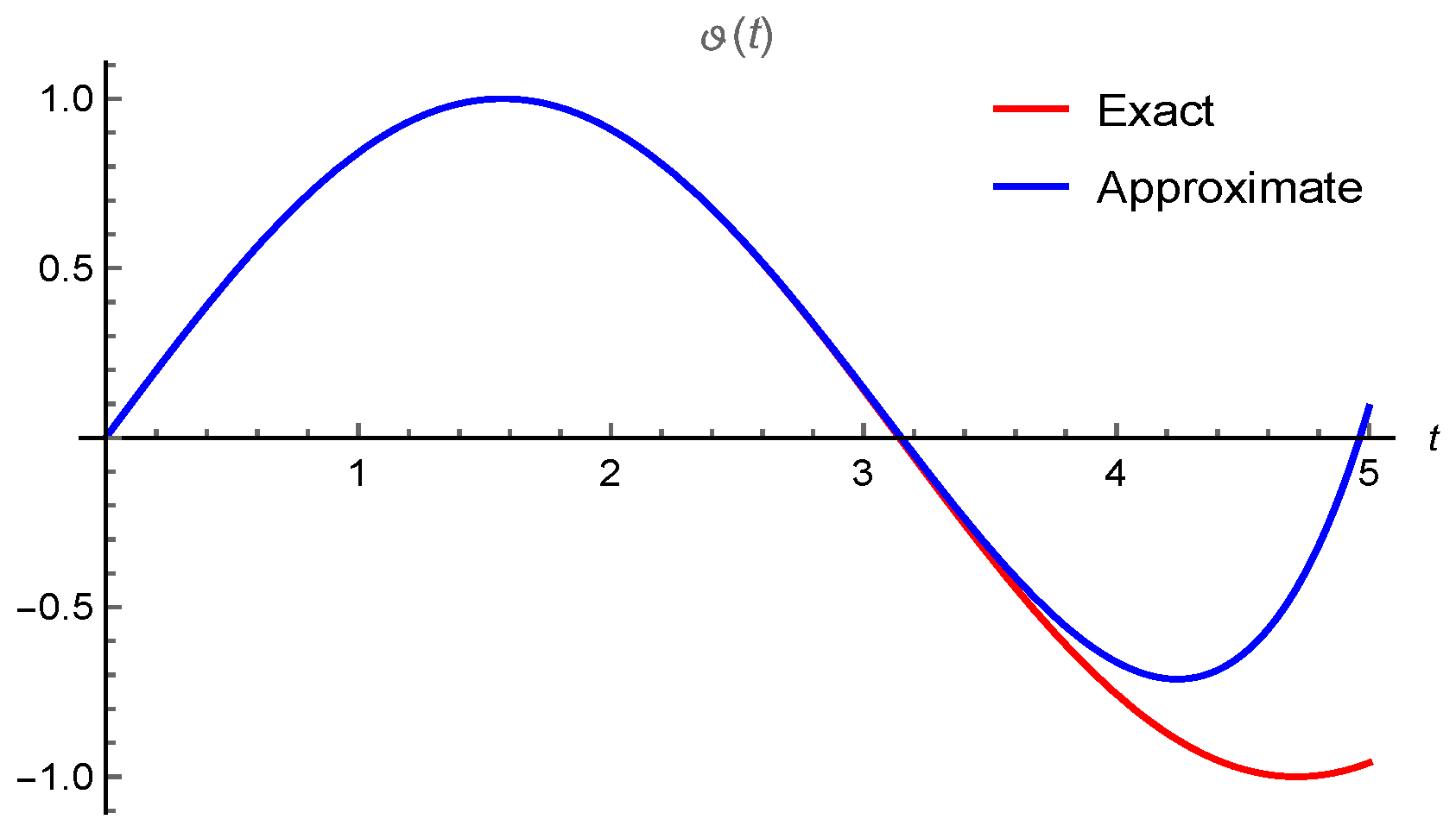
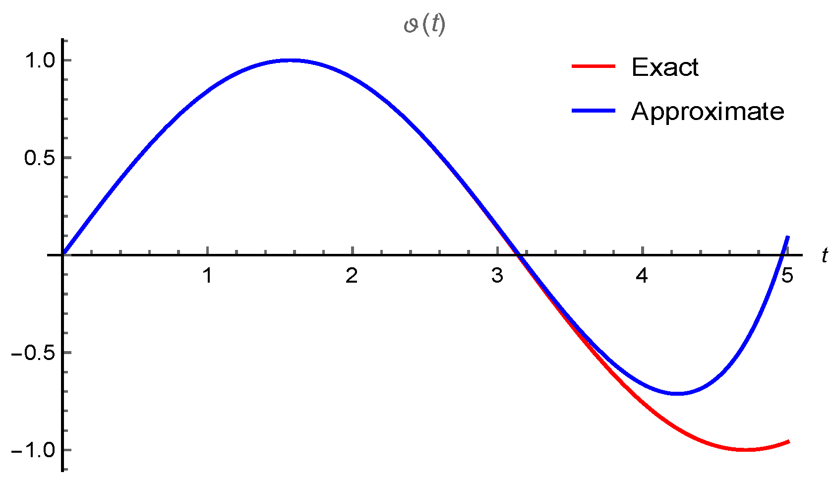
In Figure 2, we demonstrate the graphical error among the analytical solution obtained by SIS and the precise solution of Section 5.2 at $0\le t\le 8$. The graphical results show that the analytical and the exact solutions are very close to each others. It seems that the suggested approach is very efficient and authentic for finding the analytical view of nonlinear DDEqs.

5.3. Example 3

Consider a nonlinear 2nd order DDEq

$$\begin{array}{c}\hfill {\vartheta }^{\prime \prime }\left(t\right)=-\vartheta \left(t\right)+5{\vartheta }^2\left(\frac{t}{2}\right),\end{array}$$

(30)

with the initial condition

$$\begin{array}{c}\hfill \vartheta \left(0\right)=1,{\vartheta }^{\prime }\left(0\right)=-2.\end{array}$$

(31)

Using ST on Equation (30) and then evaluating, we get

$$\begin{array}{c}\hfill \frac{R\left(\theta \right)}{{\theta }^2}-\frac{\vartheta \left(0\right)}{{\theta }^3}-\frac{{\vartheta }^{\prime }\left(0\right)}{{\theta }^2}=S[-\vartheta \left(t\right)+5{\vartheta }^2\left(\frac{t}{2}\right)].\end{array}$$

Using initial condition, we get

$$\begin{array}{c}\hfill R\left(\theta \right)=\frac{1}{\theta }-2-S[\vartheta \left(t\right)-5{\vartheta }^2\left(\frac{t}{2}\right)].\end{array}$$

(32)

Applying inverse ST on Equation (32), we obtain

$$\begin{array}{c}\hfill \vartheta \left(t\right)=1-2t-S^{-1}\left[{\theta }^{2}S\left\{\vartheta \left(t\right)-5{\vartheta }^2\left(\frac{t}{2}\right)\right\}\right].\end{array}$$

(33)

Now, we use HPM on above equation, we get

$$\begin{array}{c}\hfill \sum _{i=0}^{\infty }{p}^i{\vartheta }_i\left(n\right)=1-2t-S^{-1}\left[{\theta }^{2}S\left\{\sum _{i=0}^{\infty }{p}^i{\vartheta }_i\left(t\right)-5\sum _{i=0}^{\infty }{p}^i{\vartheta }_i^2\left(\frac{t}{2}\right)\right\}\right].\end{array}$$

(34)

We are now able to compare the similar power of p to get the series such as

$$\begin{array}{cc}\hfill p^0& :{\vartheta }_0\left(t\right)=1-2t,\hfill \\ \hfill p^1& :{\vartheta }_1\left(t\right)=-S^{-1}\left[{\theta }^{2}S\left\{{\vartheta }_0\left(t\right)-5{\vartheta }_0^2\left(\frac{t}{2}\right)\right\}\right]=2t^2-\frac{4}{3}{t}^3-\frac{5}{6}{t}^4,\hfill \\ \hfill p^2& :{\vartheta }_2\left(t\right)=-S^{-1}\left[{\theta }^{2}S\left\{2{\vartheta }_0\left(\frac{t}{2}\right){\vartheta }_1\left(\frac{t}{2}\right)\right\}\right]=\frac{1}{4}{t}^4-\frac{7}{20}{t}^5+\frac{21}{576}{t}^6-\frac{5}{126}{t}^7,\hfill \\ \hfill & ⋮.\hfill \end{array}$$

On proceeding this process,

$$\begin{array}{c}\hfill \begin{array}{cc}\hfill \vartheta \left(t\right)& ={\vartheta }_0\left(t\right)+{\vartheta }_1\left(t\right)+{\vartheta }_2\left(t\right)+{\vartheta }_3\left(t\right)+{\vartheta }_4\left(t\right)+\cdots ,\hfill \\ \hfill & =1-2t+2t^2-\frac{4}{3}{t}^3+\frac{2}{3}{t}^4-\frac{7}{20}{t}^5+\frac{21}{576}{t}^6-\frac{5}{126}{t}^7+\cdots .\hfill \end{array}\end{array}$$

(35)

which yields

$$\begin{array}{c}\hfill \vartheta \left(t\right)=e^{-2t}.\end{array}$$

(36)

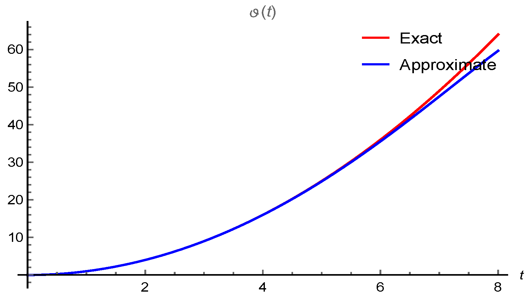
In Figure 3, we demonstrate the graphical error among the analytical solution obtained by SIS and the precise solution of Section 5.3 at $0\le t\le 1$. The graphical results show that the analytical and the exact solutions are very close to each other. It seems that the suggested approach is very efficient and authentic for finding the analytical view of nonlinear DDEqs.

5.4. Example 4

Consider a nonlinear 3rd order DDEq

$$\begin{array}{c}\hfill {\vartheta }^{‴}\left(t\right)=2{\vartheta }^2\left(\frac{t}{2}\right)-1,\end{array}$$

(37)

with the initial condition

$$\begin{array}{c}\hfill \vartheta \left(0\right)=0,{\vartheta }^{\prime }\left(0\right)=1,{\vartheta }^{″}\left(0\right)=0.\end{array}$$

(38)

Using ST on Equation (37) and then evaluating, we get

$$\begin{array}{c}\hfill \frac{R\left(\theta \right)}{{\theta }^3}-\frac{\vartheta \left(0\right)}{{\theta }^4}-\frac{{\vartheta }^{\prime }\left(0\right)}{{\theta }^3}-\frac{{\vartheta }^{″}\left(0\right)}{{\theta }^2}=S[2{\vartheta }^2\left(\frac{t}{2}\right)-1].\end{array}$$

Using the initial condition, we get

$$\begin{array}{c}\hfill \frac{R\left(\theta \right)}{{\theta }^3}-\frac{1}{{\theta }^3}=S\left[2{\vartheta }^2\left(\frac{t}{2}\right)\right]-\frac{1}{\theta }.\end{array}$$

Hence $R\left(\theta \right)$ is evaluated as

$$\begin{array}{c}\hfill R\left(\theta \right)=1-{\theta }^2+{\theta }^{3}S\left[2{\vartheta }^2\left(\frac{t}{2}\right)\right].\end{array}$$

(39)

Applying inverse ST on Equation (39), we obtain

$$\begin{array}{c}\hfill \vartheta \left(t\right)=t-\frac{t^3}{6}+S^{-1}\left[{\theta }^{3}S\left\{2{\vartheta }^2\left(\frac{t}{2}\right)\right\}\right].\end{array}$$

(40)

Now, we use HPM on the above equation, and obtain

$$\begin{array}{c}\hfill \sum _{i=0}^{\infty }{p}^i{\vartheta }_i\left(t\right)=t-\frac{t^3}{6}+S^{-1}\left[2{\theta }^{3}S\left\{\sum _{i=0}^{\infty }{p}^i{\vartheta }_i^2\left(\frac{t}{2}\right)\right\}\right].\end{array}$$

(41)

We are now able to compare the similar powers of p to get a series such as

$$\begin{array}{cc}\hfill p^0& :{\vartheta }_0\left(t\right)=t-\frac{t^3}{6},\hfill \\ \hfill p^1& :{\vartheta }_1\left(t\right)=S^{-1}\left[2{\theta }^{3}S\left\{{\vartheta }_0^2\left(\frac{t}{2}\right)\right\}\right]=\frac{t^5}{120}-\frac{t^7}{5040},\hfill \\ \hfill p^2& :{\vartheta }_2\left(t\right)=S^{-1}\left[2{\theta }^{3}S\left\{2{\vartheta }_0\left(\frac{t}{2}\right){\vartheta }_1\left(\frac{t}{2}\right)\right\}\right]=\frac{t^9}{362,880}-\frac{t^{11}}{39,916,800},\hfill \\ \hfill & ⋮.\hfill \end{array}$$

On proceeding this process,

$$\begin{array}{c}\hfill \begin{array}{cc}\hfill \vartheta \left(t\right)& ={\vartheta }_0\left(t\right)+{\vartheta }_1\left(t\right)+{\vartheta }_2\left(t\right)+{\vartheta }_3\left(t\right)+{\vartheta }_4\left(t\right)+\cdots ,\hfill \\ \hfill & =t-\frac{t^3}{3!}+\frac{t^5}{5!}-\frac{t^7}{7!}+\frac{t^9}{9!}-\frac{t^{11}}{11!}+\cdots .\hfill \end{array}\end{array}$$

(42)

which yields

$$\begin{array}{c}\hfill \vartheta \left(t\right)=sin\left(t\right).\end{array}$$

(43)

In Figure 4, we demonstrate the graphical error among the analytical solution obtained by SIS and the precise solution of Section 5.4 at $0\le t\le 5$. The graphical results show that the analytical and the exact solutions are very close to each other. It seems that the suggested approach is very efficient and authentic for finding the analytical view of nonlinear DDEqs.

6. Conclusions

In the present study, we successfully obtain the approximate solution of delay differential equations using a Sawi iterative scheme. We observe that the Sawi transform deals with the recurrence relation without any hypothesis and the discretization of the variables whereas HPM allows a better strategy to establish the rate of convergence of the series solution. The initial conditions help us to derive the iteration terms of the illustrated problems. We obtain a successive series solution that converges to the exact solution very swiftly. All the calculations and the graphical representation are made with Mathematica software. These graphical representations show that SIS is ultimately appropriate for nonlinear DDEqs. We predict that this strategy is helpful for other nonlinear fractional DDEqs and we aim to investigate their solution with fast convergence the future research.

References

- Rezazadeh, H.; Younis, M.; Eslami, M.; Bilal, M.; Younas, U. New exact traveling wave solutions to the (2+ 1)-dimensional chiral nonlinear schrödinger equation. Math. Model. Nat. Phenom. 2021, 16, 38. [Google Scholar] [CrossRef]
- Eslami, M. Exact traveling wave solutions to the fractional coupled nonlinear schrodinger equations. Appl. Math. Comput. 2016, 285, 141–148. [Google Scholar] [CrossRef]
- Gepreel, K.A.; Nofal, T.A.; Al-Thobaiti, A.A. The modified rational jacobi elliptic functions method for nonlinear differential difference equations. J. Appl. Math. 2012, 2012, 427479. [Google Scholar] [CrossRef] [Green Version]
- Georgieva, A.; Pavlova, A. Fuzzy sawi decomposition method for solving nonlinear partial fuzzy differential equations. Symmetry 2021, 13, 1580. [Google Scholar] [CrossRef]
- Islam, R.; Alam, M.N.; Hossain, A.; Roshid, H.; Akbar, M. Traveling wave solutions of nonlinear evolution equations via exp (-ϕ (η))-expansion method. Glob. J. Sci. Front. Res. 2013, 13, 63–71. [Google Scholar]
- Eslami, M.; Rezazadeh, H. The first integral method for wu–zhang system with conformable time-fractional derivative. Calcolo 2016, 53, 475–485. [Google Scholar] [CrossRef]
- Raslan, K.; Ali, K.K.; Shallal, M.A. The modified extended tanh method with the riccati equation for solving the space-time fractional ew and mew equations, Chaos. Solitons Fractals 2017, 103, 404–409. [Google Scholar] [CrossRef]
- Nejla, G.; Emine, G.K.; Yusuf, G. Chebyshev-tau method for the linear klein-gordon equation. Int. J. Phys. Sci. 2012, 7, 5723–5728. [Google Scholar]
- Rezazadeh, H.; Ullah, N.; Akinyemi, L.; Shah, A.; Mirhosseini-Alizamin, S.M.; Chu, Y.-M.; Ahmad, H. Optical soliton solutions of the generalized non-autonomous nonlinear schrödinger equations by the new kudryashov’s method. Results Phys. 2021, 24, 104179. [Google Scholar] [CrossRef]
- Gepreel, K.A.; Al-Thobaiti, A. Exact solutions of nonlinear partial fractional differential equations using fractional sub-equation method. Indian J. Phys. 2014, 88, 293–300. [Google Scholar] [CrossRef]
- Althobaiti, A.; Althobaiti, S.; El-Rashidy, K.; Seadawy, A.R. Exact solutions for the nonlinear extended kdv equation in a stratified shear flow using modified exponential rational method. Results Phys. 2021, 29, 104723. [Google Scholar] [CrossRef]
- Cakmak, M.; Alkan, S. A numerical method for solving a class of systems of nonlinear pantograph differential equations. Alex. Eng. J. 2022, 61, 2651–2661. [Google Scholar] [CrossRef]
- Nuruddeen, R.I.; Aboodh, K.S.; Ali, K.K. Analytical investigation of soliton solutions to three quantum zakharov-kuznetsov equations. Commun. Theor. Phys. 2018, 70, 405. [Google Scholar] [CrossRef]
- Alaroud, M.; Al-Smadi, M.; Ahmad, R.R.; Din, U.K.S. An analytical numerical method for solving fuzzy fractional volterra integro-differential equations. Symmetry 2019, 11, 205. [Google Scholar] [CrossRef] [Green Version]
- Duan, J.-S.; Rach, R.; Wazwaz, A.-M. Higher order numeric solutions of the lane–emden-type equations derived from the multi-stage modified adomian decomposition method. Int. J. Comput. Math. 2017, 94, 197–215. [Google Scholar] [CrossRef]
- Dehghan, M.; Salehi, R. Solution of a nonlinear time-delay model in biology via semi-analytical approaches. Comput. Phys. Commun. 2010, 181, 1255–1265. [Google Scholar] [CrossRef]
- Luo, X.; Habib, M.; Karim, S.; Wahash, H.A. Semianalytical approach for the approximate solution of delay differential equations. Complexity 2022, 2022, 1049561. [Google Scholar] [CrossRef]
- Khan, H.; Liao, S.-J.; Mohapatra, R.; Vajravelu, K. An analytical solution for a nonlinear time-delay model in biology. Commun. Nonlinear Sci. Numer. Simul. 2009, 14, 3141–3148. [Google Scholar] [CrossRef]
- Xu, M.-Q.; Lin, Y.-Z. Simplified reproducing kernel method for fractional differential equations with delay. Appl. Math. Lett. 2016, 52, 156–161. [Google Scholar] [CrossRef]
- Anakira, N. A new accurate procedure for solving nonlinear delay differential equations. J. Math. Comput. Sci. 2021, 11, 4673–4685. [Google Scholar]
- He, J.-H. Homotopy perturbation technique. Comput. Methods Appl. Mech. Eng. 1999, 178, 257–262. [Google Scholar] [CrossRef]
- He, J.-H. Homotopy perturbation method: A new nonlinear analytical technique. Appl. Math. Comput. 2003, 135, 73–79. [Google Scholar] [CrossRef]
- Khuri, S.A.; Sayfy, A. A laplace variational iteration strategy for the solution of differential equations. Appl. Math. Lett. 2012, 25, 2298–2305. [Google Scholar] [CrossRef]
- Nadeem, M.; Li, F. He–laplace method for nonlinear vibration systems and nonlinear wave equations, Journal of Low Frequency Noise. Vib. Act. Control. 2019, 38, 1060–1074. [Google Scholar]
- Ganji, D.; Sadighi, A. Application of he’s homotopy-perturbation method to nonlinear coupled systems of reaction-diffusion equations. Int. J. Nonlinear Sci. Numer. Simul. 2006, 7, 411–418. [Google Scholar] [CrossRef]
- Mishra, R.; Aggarwal, S.; Chaudhary, L.; Kumar, A. Relationship between sumudu and some efficient integral transforms. Int. J. Innov. Technol. Explor. Eng. 2020, 9, 153–159. [Google Scholar] [CrossRef]
- Attaweel, M.E.; Almassry, H.A. A new application of sawi transform for solving volterra integral equations and volterra integro-differential equations. Libyan J. Sci. 2019, 22, 64–77. [Google Scholar]
- Singh, G.P.; Aggarwal, S. Sawi transform for population growth and decay problems, International Journal of Latest Technology in Engineering. Manag. Appl. Sci. 2019, 8, 157–162. [Google Scholar]
- Higazy, M.; Aggarwal, S. Sawi transformation for system of ordinary differential equations with application. Ain Shams Eng. J. 2021, 12, 3173–3182. [Google Scholar] [CrossRef]
- Nadeem, M.; He, J.-H. The homotopy perturbation method for fractional differential equations: Part 2, two-scale transform. Int. J. Numer. Methods Heat Fluid Flow 2021, 32, 559–567. [Google Scholar] [CrossRef]
- Biazar, J.; Ghazvini, H. Convergence of the homotopy perturbation method for partial differential equations. Nonlinear Anal. Real World Appl. 2009, 10, 2633–2640. [Google Scholar] [CrossRef]
- MTurkyilmazoglu, M. Convergence of the homotopy perturbation method. Int. J. Nonlinear Sci. Numer. Simul. 2011, 12, 9–14. [Google Scholar] [CrossRef]
Figure 1.
2D graphical error of at .
Figure 2.
Figure 3.
Figure 4.
Publisher’s Note: MDPI stays neutral with regard to jurisdictional claims in published maps and institutional affiliations. |
© 2022 by the authors. Licensee MDPI, Basel, Switzerland. This article is an open access article distributed under the terms and conditions of the Creative Commons Attribution (CC BY) license (https://creativecommons.org/licenses/by/4.0/).
Share and Cite
MDPI and ACS Style
Nadeem, M.; Edalatpanah, S.A.; Mahariq, I.; Aly, W.H.F. Analytical View of Nonlinear Delay Differential Equations Using Sawi Iterative Scheme. Symmetry 2022, 14, 2430. https://doi.org/10.3390/sym14112430
AMA Style
Nadeem M, Edalatpanah SA, Mahariq I, Aly WHF. Analytical View of Nonlinear Delay Differential Equations Using Sawi Iterative Scheme. Symmetry. 2022; 14(11):2430. https://doi.org/10.3390/sym14112430
Chicago/Turabian StyleNadeem, Muhammad, Seyyed Ahmad Edalatpanah, Ibrahim Mahariq, and Wael Hosny Fouad Aly. 2022. "Analytical View of Nonlinear Delay Differential Equations Using Sawi Iterative Scheme" Symmetry 14, no. 11: 2430. https://doi.org/10.3390/sym14112430
Note that from the first issue of 2016, this journal uses article numbers instead of page numbers. See further details here.