Prediction of Marshall Stability and Marshall Flow of Asphalt Pavements Using Supervised Machine Learning Algorithms

Abstract

The conventional method for determining the Marshall Stability (MS) and Marshall Flow (MF) of asphalt pavements entails laborious, time-consuming, and expensive laboratory procedures. In order to develop new and advanced prediction models for MS and MF of asphalt pavements the current study applied three soft computing techniques: Artificial Neural Network (ANN), Adaptive Neuro-Fuzzy Inference System (ANFIS), and Multi Expression Programming (MEP). A comprehensive database of 343 data points was established for both MS and MF. The nine most significant and straightforwardly determinable geotechnical factors were chosen as the predictor variables. The root squared error (RSE), Nash–Sutcliffe efficiency (NSE), mean absolute error (MAE), root mean square error (RMSE), relative root mean square error (RRMSE), coefficient of determination (R²), and correlation coefficient (R), were all used to evaluate the performance of models. The sensitivity analysis (SA) revealed the rising order of input significance of MS and MF. The results of parametric analysis (PA) were also found to be consistent with previous research findings. The findings of the comparison showed that ANN, ANFIS, and MEP are all reliable and effective methods for the estimation of MS and MF. The mathematical expressions derived from MEP represent the novelty of MEP and are relatively reliable and simple. R_overall values for MS and MF were in the order of MEP > ANFIS > ANN with all values over the permissible range of 0.80 for both MS and MF. Therefore, all the techniques showed higher performance, possessed high prediction and generalization capabilities, and assessed the relative significance of input parameters in the prediction of MS and MF. In terms of training, testing, and validation data sets and their closeness to the ideal fit, i.e., the slope of 1:1, MEP models outperformed the other two models. The findings of this study will contribute to the choice of an appropriate artificial intelligence strategy to quickly and precisely estimate the Marshall Parameters. Hence, the findings of this research study would assist in safer, faster, and more sustainable predictions of MS and MF, from the standpoint of time and resources required to perform the Marshall tests.

1. Introduction

To endure climate conditions and traffic loads, various types of bituminous mixes are used for roadway pavements which must be effectively designed as bitumen and aggregate mixtures. Inadequate mechanical characteristics could lead to a variety of problems in road pavements such as low temperature or fatigue cracks, stripping, permanent deformations, etc. Such failure mechanisms reduce the pavement’s service life and pose major safety concerns for road users [1]. Consequently, it is critical to characterize the performance of mixtures in terms of their composition so that optimization based on performance might be done during the mix design process [2,3,4]. Experimental methods are currently utilized to assess the performance of bituminous mixes [5,6,7,8,9,10], which necessitate costly laboratory experiments in conjunction with skilled labor. As a result, any change in the composition of mixtures, whether it be in bitumen content or type or aggregate gradation, necessitates additional laboratory testing, increasing cost and time in the design process.

Numerous researchers have been working on developing numerical or mathematical relationships for the mechanical behavior of bituminous mixes that can quickly produce reliable and accurate predicted results for bituminous mixes. Advanced machine learning (ML) methods allow in-depth and rational analysis of material responses [11,12,13,14,15,16,17,18,19,20]. ML techniques have gained significant popularity in research due to their high reliability and prediction capabilities despite the fact that they are not based on physical testing procedures and they are being utilized in modeling and forecasting the complex behaviors of several pavement engineering materials [21,22,23,24,25,26]. Data mining procedures in material, civil, and pavement engineering, in particular, have been reported widely in the previous two decades, thanks to the swift development in the approaches of ML [27]. The soft computing methods (SCMs) or artificial intelligence techniques (AITs) that are developed recently, for example, artificial neural networks (ANNs) (sub-types are; multilayer perceptron neural network (MLPNN), Bayesian neural network (BNN), general regression neural network (GRNN), backpropagation neural network (BPNN), and k-nearest neighbor (KNN)), ANNs with their hybrid form, i.e., support vector machine (SVM), multivariate adaptive regression splines (MARS), eXtreme gradient boosting (XGBoost), adaptive neuro-fuzzy inference system (ANFIS), alternate decision trees), genetic algorithms (GAs), M5 model trees, evolutionary algorithms (EAs), ensemble random forest regression (ERFR), genetic expression programming (GEP), and MEP, have facilitated in the development of the various models in conjunction with conventional statistical models, e.g., regression, among many others [25,28,29,30,31,32,33,34,35,36,37,38]. Mechanistic learning has been frequently used to evaluate the estimating models for the development of intelligent structures [39]. Moreover, Giustolisi et al. (2007) suggested the categorization of different mathematical models into grey, black, and white colors [40]. The known parameters and variables, the white-box model (first type), are established on the basis of physical laws forming precise physical relationships, hence maximum transparency is provided. Although, it was argued by Shahin et al. (2009) that their underlying procedure is not entirely understood, making the formulation challenging and difficult [41]. Additionally, black box models depend on regressive data-driven techniques with unidentified functional forms of relationships among respective parameters that must be estimated. Finally, in grey-box models, it can be labelled as logical systems where mathematical frameworks more successfully assess the system’s behavior. The ANFIS and ANN due to (i) low transparency, (ii) the incapability to describe the underlying physical process, explicitly, and (iii) the inability to develop expressions of closed-form, are both classified as “black-box” models [42]. MEP, on the other hand, is categorized as a “grey-box model”, since its approach is simple and straightforward in order to conceptualize the physical phenomenon [43]. In the field of pavement engineering, although it is considered that the performance of models based on is decent while using ANFIS and ANN, on the other hand, MEP has also shown very good results [44], for which a comparative study needs to be conducted to verify the assumptions made and to gain further insights. With these uncertainties in sight, the current research study integrates ANN, ANFIS, and MEP to evaluate their ability to predict the MF and MS of asphalt pavements.

First and foremost, ANNs are problem-solving computational models, inspired by biological neural networks (NNs) that aim to mimic the biological structure of our nervous system and brain [29,45,46]. ANNs explicitly record the link between the corresponding input and output variables of the models [47], but they do not develop an empirical formulation, which limits their real-world applicability despite their better accuracy [39,48]. Secondly, Jang (1993) introduced ANFIS, a fuzzy inference system of the Sugeno or Takagi Sugeno Kang (TSK) type, based on the principle of ANNs [49,50]. ANFIS is a hybrid model that integrates both fuzzy algorithms and ANNs. It is vital to note that fuzzy logic (FL) incorporates elements of falsehood and truth and does not behave in the same way as 1′s and 0′s logic [51]. Lastly, MEP, a method of genetic programming (GP), has been proven as an efficient and alternative approach in the prediction of complex and nonlinear problems [44]. Oltean and Dumitrescu (2002) were the first ones to suggest the MEP approach [52]. The problem of having several computer programs could be encoded into a single chromosome using this method. Through computation procedure, the best encoded predicting expression can be constructed and easily changed to meet the practical applications. The development of prediction models using the MEP approach has seen a rise in the previous decade due to its advantage of easy implementation, high efficiency, and prediction accuracy, in the field of material engineering. This method has been successfully used to forecast the tensile and compressive strength [53], Marshall parameters [44], classification of soil [54], reloading and secant moduli of soil deformation [55], peak ground acceleration [56], etc. Hence, MEP is feasible to estimate the MS and MF of asphalt pavements, which is reinforced by past relevant research studies of this method on specific material engineering problems.

Traditional statistical studies were used to derive prior correlations for the MS and MF of asphalt pavements, which had shortcomings such as: (i) fewer data points, (ii) governing parameters had smaller correlations, and (iii) the absence of an integrated comparative evaluation, among others [42]. Furthermore, the test of MS and MF takes time, while their determination in the laboratory is also time-consuming and costly [57,58]. A number of studies have previously employed basic input parameters for the prediction of the MS and MF of asphalt pavements using ANN and ANFIS approaches [57,59,60,61,62,63,64,65,66]. As a result, the goal of this research study is the construction of models that reliably predict the MS and MF of asphalt pavements using major input parameters that are determined simply and economically. Three soft computing approaches, i.e., ANN, ANFIS, and MEP, were used to construct prediction expressions for MS and MF. Eight properties were used in input parameters, i.e., Percentage of Aggregates (P_s), Percentage Asphalt Content (P_b), Bulk Specific Gravity of Compacted Aggregate (G_mb), Bulk Specific Gravity of Aggregate (G_sb), Maximum Specific Gravity Paving Mix (G_mm), Percentage of Voids in Mineral Aggregate (VMA), Percentage of Air Voids (V_a), and Percentage Voids Filled by Bitumen (VFA). MS (Corrected Stability in Kg), and MF (Flow in 0.25 mm) were the output parameters of this study. The major objectives of this research study were (i) the construction of MEP-based prediction expressions, (ii) the investigation of the feasibility study for ANN and ANFIS approaches, and (iii) the comparison of the MEP-based model with models of ANN, and ANFIS, for prediction of MS and MF. 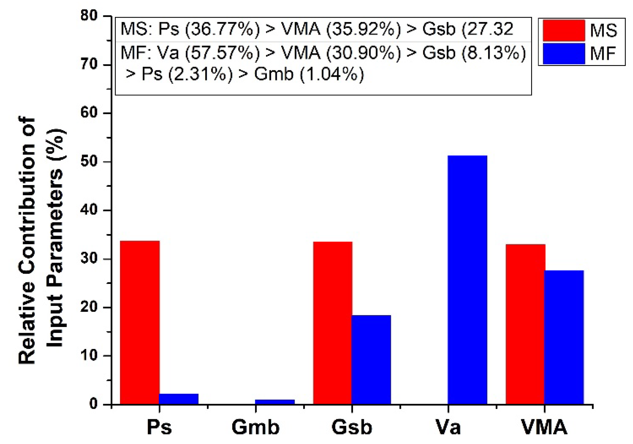The ANN, ANFIS, and MEP models were evaluated by means of several statistical error checks, such as root square error (RSE), Nash–Sutcliffe efficiency (NSE), mean absolute error (MAE), relative root mean square error (RRMSE), regression coefficient (R²), and correlation coefficient (R). Furthermore, PA was performed, and results were evaluated to determine the negative and positive effects of input variables by employing sensitivity analysis.

2. Overview of Soft-Computing Approaches

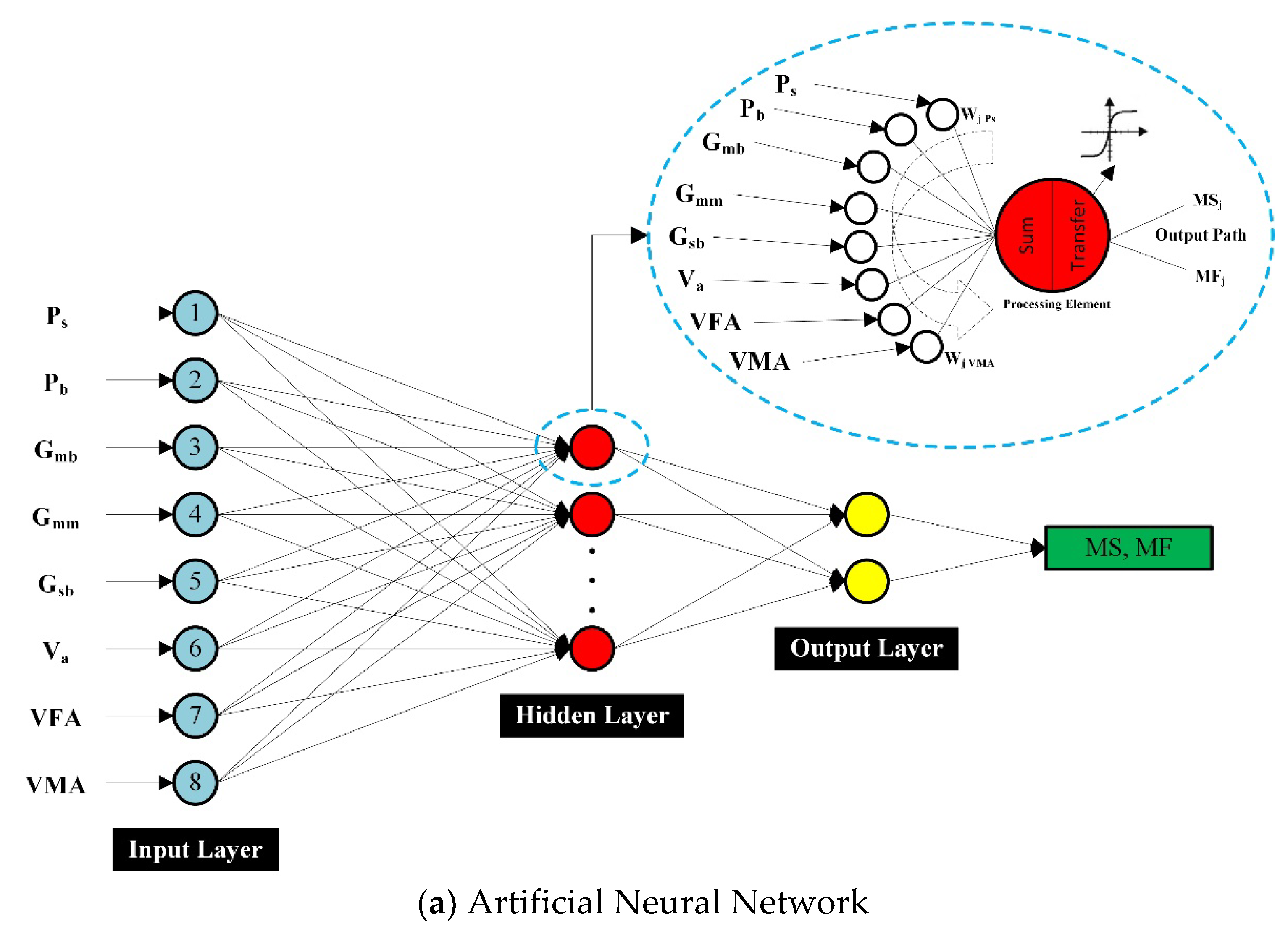
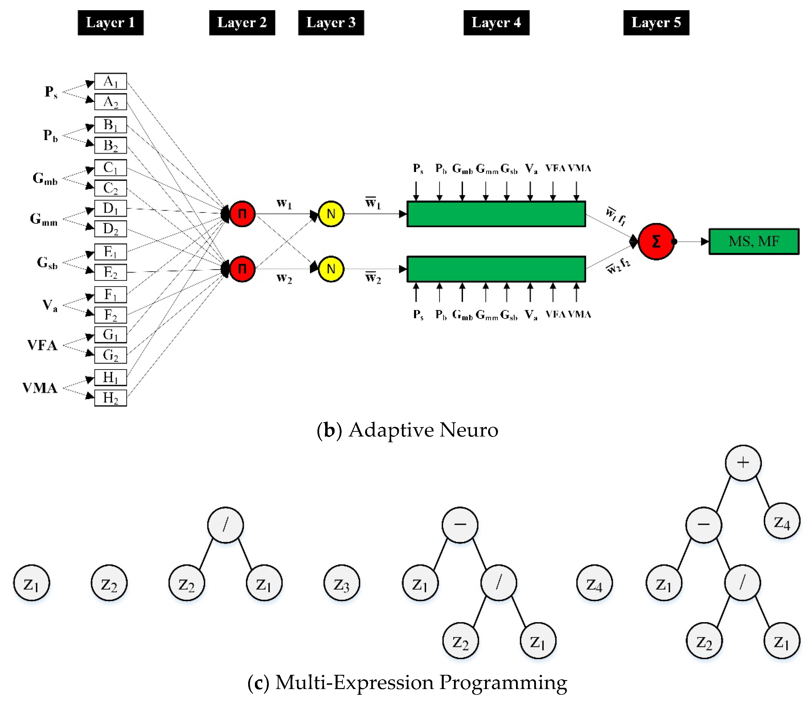
ANNs are computer algorithms that can accurately forecast and categorize data-processing challenges [67,68,69]. They consist of mathematical models based on the properties of biological neuron networks that are similar to the human brain [51,70]. ANNs have layered structures which have diversified arrangements of processing elements (PEs) or nodes; (i) an input layer consisting of an independent set of parameters, (ii) a hidden layer(s) consisting of various hidden parameters better known as hidden neurons, and (iii) an output layer, which consists of target parameters (Figure 1a) [39,71]. Eight different characteristics of asphalt concrete were chosen as the input parameter for the prediction of the corresponding output parameters, i.e., MS and MF, as shown in Figure 1. Each individual input parameter in the preceding layer was multiplied by the appropriate connection weight, in a hidden layer. On each node, the sum of weighted input signals is added with a cutoff value (θ_j). The collected input (I_j) then goes through a transfer function (nonlinear) in the transfer phase. Linear, sigmoid, logistic, hyperbolic, and stepped are among the most frequently utilized activation transfer functions (ATFs) [39,72]. ATF is a major and significant characteristic of NNs, and it has a considerable impact on the functioning of the ANN model as it helps in the induction of nonlinearity to NNs, implying that selecting a feasible ATF is of critical importance [73]. Multi-state activation functions (MSAFs) were previously utilized in the improvement of deep neural networks (DNNs) models [74], softmax ATFs [75], swish ATFs [76], the tangent hyperbolic and logistic sigmoid ATFs [77], ATFs of transcendental type parametric algebraic [78], etc. In this research study, more specifically, PURELIN (linear–transfer–function), and TRANSIG (BPNN’s transfer functions with an output ranging from +1 to −1, and are related to bipolar sigmoid), are utilized in order to increase the number of the transfer function as well as neurons in each layer, thus helping to improve the statistical measures for the training set, but lowering the precision of testing and validation datasets [79,80,81]. Dorofki et al. (2012) discovered, by applying several statistical parameters, that the performance of Log-sigmoid (transfer function) was determined as the best, as it is differentiable, bounded, and continuous. However, Purelin (transfer function) yielded even further improved results [82]. Accordingly, PE (MSj or MFj) is acquired as the subsequent output parameter. It is essential to specify here that the output of the first PE contributes to the input of the next PE. For the output layer and hidden layer, each neuron performs the logistic function in Equation (1), which was utilized as the AF [83]. Additionally, Equations (1)–(3) show the procedure mentioned above.

$$f_h\left(z\right)=\frac{1}{1+e^{-z}}$$

(1)

$$I_j=\left\{\left(w_{j P_s }\times P_s+w_{j P_b}\times P_b+w_{j G_{mb}}\times G_{mb}\dots w_{j VMA}\times VMA\right)\right\}+{\theta }_j \mathrm{Summation}$$

(2)

$$M{S}_j or M{F}_j=f\left(I_j\right) \mathrm{Transfer}$$

(3)

The learning or training phase begins when the propagation of information is started by the ANNs from the input layer, and then weights are updated, consistent with the predefined rules, in order to find the best combination of weights to yield the least amount of error possible. Then a new testing set is utilized to validate the trained model. More details of the technique and the evolution of ANN modelling are explained in greater length elsewhere and are outside the scope of this study [39,46,84,85,86,87,88].

An intriguing computational intelligence modeling method, ANFIS, blends generalization capability of ANNs with FL’s reasoning capability. ANFIS has an enhanced estimating ability and is an effective substitute for the computation of complex and nonlinear problems with high accuracy [89,90,91]. It uses training data for learning with any sophisticated mathematical model, then generates the results onto a fuzzy inference system (FIS), similar to ANNs [70,92]. Similar to the process used by ANNs, the ANFIS tool in MATLAB R2020b starts training output and input variables for the evaluation of output and input mapping. A simple FIS consists of several processes, one of which is the entering of inputs to aid the fuzzification of fuzzy sets according to the activation of linguistic rules. Following this, particular guidelines are either established by a professional or could be derived from arithmetic data. Inference is the succeeding step that involves the mapping of fuzzy sets according to predefined rules. The final output values are obtained once fuzzy sets have been defuzzified. To put it another way, the ANFIS approach is made up of five basic stages: (i) datasets, (ii) development of ANFIS, (iii) setting of variables, (iv) training and validating the datasets, and (v) outputs or results. Additionally, Figure 1b, shows the architecture of ANFIS for eight input parameters (P_s, P_b, G_sb, G_mb, G_mm, VMA, V_a, and VFA) with circles and squares denoting the fixed and adaptive nodes, respectively. The first-order of the Sugeno model depicts ANFIS architecture, by using two IF-THEN rules.

Tue Rules:

Rule 1: IF (P_s is A₁) and (P_b is B₁)

Then, Equation (4) states that,

{f₁ = p₁(P_s) + q₁(P_b) + r₁}

(4)

Rule 2: IF (P_s is A₂) and (P_b is B₂)

Then, according to Equation (5)

{f₂ = p₂(P_s) + q₂(P_b) + r₂}

(5)

where f_n denotes the fuzzy output (MS and MF) for input (P_s, P_b, G_mb … VFA) to the fuzzy extent, A_n and B_n denote the sets of fuzzy, and p_n, r_n, and q_n denote the parameters for shape derived during the training period.

An ANFIS model is made up of five layers [90], as can be shown. These layers and their functions are described in detail here.

Layer 1: the adaptive PEs in the first layer, known as the fuzzification layer, produce outputs in the form of Equations (6) and (7) which explains the functions of the fuzzy membership of the model’s input variables, and the base of initial fuzzy rule, as follows;

$$O_i^1={\mu }_{Ai}\left(P_s\right), \mathrm{i} =1, 2$$

(6)

$$O_i^1={\mu }_{Bi-2}\left(P_b\right), \mathrm{i} =3, 4$$

(7)

where μ represents the weight obtained while linking the function of fuzzy membership, and ${\mu }_{Ai}\left(P_s\right)$ in conjunction with ${\mu }_{Bi-2}\left(P_b\right)$ discriminates the method of implementing the function of fuzzy membership. Equation (8) states ${\mu }_{Ai}\left(P_s\right)$ for a function of the bell-shaped membership,

$${\mu }_{Ai}\left(P_s\right)=\frac{1}{1+{\left(\frac{P_s-c_i}{a_i}\right)}^{b^i}}$$

(8)

where a_i, b_i, and c_i are the parameters impacting the function of the membership.

Layer 2: This layer’s output is predefined rules’ firing strength for a pattern of specified input. The nodes in the second layer perform basic multiplication and are constant, with output variables as follows (Equation (9)),

$$O_i^2=w_i={\mu }_{Ai}\left(P_s\right)·{\mu }_{Bi}\left(P_b\right) \mathrm{i} =1, 2$$

(9)

Layer 3: The nodes in this layer are fixed and are similar as they were in the second layer, such that the firing strengths of the preceding layer are normalized, and thus Equation (10) represents the outputs;

$$O_i^3=\overline{w_i}=\frac{w_i}{w_1+w_2} \mathrm{i} =1, 2$$

(10)

Layer 4: The adaptive nodes of this layer, and their outputs are characterized as products of a first-order polynomial, and normalized firing strength, with the first-order Sugeno model taken into account. Thus, the output is given by (Equation (11));

$$O_i^4=\overline{w_i}{f}_i=\overline{w_i}\left\{p_i\left(P_s\right)+q_i\left(P_b\right)+r_i\right\}$$

(11)

Layer 5: In the fifth layer, there is one fixed node (Σ) that performs the addition of weighted result of rules received from the subsequent layer, yielding the model’s output as Equation (12);

$$O_i^5={\displaystyle \sum }_{i=1}^2\overline{w_i}{f}_i=\frac{{{\displaystyle \sum }}_{i=1}^2{w}_i{f}_i}{w_1+w_2}$$

(12)

It is essential to note that only the first and fourth layers of the ANFIS architecture are adaptive. In the first layer, the three adaptive parameters, i.e., a_i, b_i, and c_i (premise-parameters) are linked to functions of input membership. Likewise, the three adaptable variables, i.e., p_i, q_i, and r_i, also known as consequent parameters, are found in the fourth layer, and are related to the first-order polynomial [93,94].

GAs are stochastic methods for finding and optimizing the solutions to a problem based on natural and genetic selection principles [95]. GAs generate a chain of binary strings which express the solution using traditional optimization techniques. GP was introduced by Koza, in 1992, as an extension of GAs by developing string expressions into computer-friendly programs, such as functional programming or tree structures [96,97,98]. GP is a symbolic technique of optimization that applies Darwin’s natural selection principle to computer programs for the solution of a problem. The major purpose of the GP is to find a program based on fitness function by the connection of known input parameters with known output parameters. Generally, there are three forms of GP: graph-based, linear-based, and tree-based [99,100]. The efficiency of linear-based GP is more than its other types since it does not require slow or expensive interpreters. Consequently, it allows a more appropriate value for the linear-based GP, in order to enhance the model’s precision in actual timeframes [101,102,103].

While considering accuracy and efficiency, in this investigation, linear-based GP also known as MEP was utilized to forecast the MS and MF of asphalt pavements. The MEP encodes solutions using linear chromosomes. The MEP encodes solutions using linear chromosomes. A chromosome can store various solutions (computer programs). The best of the encoded solutions, which represent the chromosome, is chosen by comparing the fitness values of the computer programs. The algorithm of MEP begins by creating computer programs of a random population. To construct the best computer program, MEP continue to follow the below-mentioned steps until it achieves the termination condition [52,104]:

• Using the binary tournament approach, two parents are chosen and recombined with a probability of fixed crossover.
• By recombining the two parents, two offspring are obtained.
• The mutation of the offspring takes place by the replacement of the best individual with the worst in the current population.

MEP is represented in the same way as C and Pascal compliers translate mathematical statements to machine code [54,99]. A string of expressions represents the genes of MEP. The length of the chromosome (length of code), which remains constant throughout the computation period, is used to determine the number of genes. Each gene has either one or two terminals (a constituent of terminal set T) as well as a function symbol (a constituent of function set F). To obtain a syntax accurate program, the first gene of the chromosome must be a terminal which is selected randomly from ‘T’. A pointer to function arguments is included in a gene containing a function. The generated terminal indices in a specific gene have lower values than the gene’s chromosome position.

The following is an illustration of the MEP chromosome:

• G₀: z₁
• G₁: z₂
• G₂: G₁/G₀
• G₃: z₃
• G₄: G₀ − G₂
• G₅: z₄
• G₆: G₄ + G₅

The terminal set T = {z₁, z₂, z₃, z₄}, and the function set F = {+, /, −} are utilized in this example. The genes of MEP can be converted into computer code by traversing the code of chromosomes from top to bottom. Figure 1c shows the relevant gene trees. G₀ = z₁, G₁ = z₂, G₃ = z₃, and G₅ = z₄ are the genes that encode a single terminal. Gene 2 denotes the operation/(division) on the operands at chromosome positions 0 and 1 with the expression G₂ = z₂/z₁. Gene 4 denotes operation subtraction on the operands at positions 0 and 2 making the expression as ${\mathrm{G}}_4={\mathrm{z}}_1-\frac{{\mathrm{z}}_2}{{\mathrm{z}}_1}$. Lastly, ${\mathrm{G}}_6={\mathrm{z}}_1-\frac{{\mathrm{z}}_2}{{\mathrm{z}}_1}+{\mathrm{z}}_4$. Hence, the chromosome could be visualized as a forest of gene trees (Figure 1c) each of which has several expressions, after determining the fitness of entire expressions in the chromosome of MEP [105].

3. Research Methodology

3.1. Data Division and Pre-Processing

Comprehensive and detailed datasets of 343 data points were developed for the development of predicting models utilizing ANN, ANFIS, and MEP approaches. The data points were acquired from numerous construction firms engaged in Pakistani road development projects. Values from 25 distinct, newly constructed road projects in Pakistan were used to create the full dataset for Asphalt Wearing Course (AWC). The Marshall Tests were carried out in recognized laboratories of numerous Pakistani construction enterprises, and they received the proper Pakistan Engineering Council’s (PEC) approval in compliance with the ASTM standard. Bitumen of grade 60/70 was used in all the collected datasets. Furthermore, all the respective tests related to bitumen, coarse and fine aggregates were conducted with their results in the range as specified according to the relevant ASTM Standards. The distribution of the datasets determines the efficacy of the developed models [29]. Characteristics of the data, the relationship between input and out parameters, and the size of the data all play critical roles in the model’s accuracy [106]. According to prior research, including too many inputs with a low correlation with output might increase the model’s complexity and have a negative impact on the performance of the model [107]. Hence, for the prediction of MS and MF, eight input parameters were chosen for ANN, ANFIS, and MEP approaches.

Table 1. Descriptive Statistics of the Input Parameters and Output Parameters utilized in ANN, ANFIS, and MEP models.

Parameters	Unit	Mean	Median	Standard Deviation	Coefficient of Variation	Minimum	Maximum	Range	Skewness	Kurtosis
OUTPUTS
MS	kg	1358	1372	109.40	8.06	1024	1680	656.000	−0.129	0.838
MF	0.25 mm	10.97	10.90	1.70	15.46	6.40	15.10	8.700	−0.057	−0.476
INPUTS
Ps	%	95.94	95.90	0.66	0.68	94.50	97.50	3.000	0.083	−0.472
Pb	%	4.06	4.10	0.66	16.16	2.50	5.50	3.000	−0.083	−0.472
Gmb	g/cm3	2.363	2.355	0.032	1.344	2.290	2.431	0.141	0.413	−0.474
Gmm	g/cm3	2.501	2.495	0.038	1.507	2.427	2.599	0.172	0.497	−0.212
Gsb	g/cm3	2.660	2.655	0.033	1.238	2.625	2.751	0.126	1.486	1.744
Va	%	5.50	5.25	1.53	27.82	2.20	9.85	7.649	0.646	−0.155
VFA	%	62.81	63.89	10.06	16.02	34.82	83.65	48.836	−0.498	−0.355
VMA	%	14.79	14.68	0.72	4.87	13.24	17.39	4.142	0.692	1.192

shows the descriptive statistics for all input parameters evaluated in this study. It shows units of all the parameters, mean and median (data center), standard deviation and coefficient of variance (dispersion), minimum and maximum (data extremes), and skewness and kurtosis (shapes of distribution), making the interpretation of the datasets relatively straightforward. The numbers in Table 1 give an understanding of the common material indices that influence the MS and MF of asphalt pavements. The MS and MF of the AWC are found to range from 1024 to 1680 and 6.40 to 15.10, respectively. The parameters shown in Table 1 are recommended for calculating the MS and MF of AWC using AI techniques in this research study.

The Spearman rank coefficient of correlation was used for determining the correlation of output parameters, i.e., MS and MF based on the distribution of all input parameters, as shown in

Table 2. Correlation for parameters of MS.

	Ps	Pb	Gmb	Gmm	Gsb	Va	VFA	VMA	MS
Ps	1
Pb	−1	1
Gmb	−0.3697	0.3697	1
Gmm	0.6758	−0.6758	0.3504	1
Gsb	0.0874	−0.0874	0.6770	0.6963	1
Va	0.9321	−0.9321	−0.5002	0.6356	0.0838	1
VFA	−0.9538	0.9538	0.4636	−0.6518	−0.0245	−0.9857	1
VMA	−0.0921	0.0921	−0.3039	−0.0874	0.3075	0.1646	−0.0035	1
MS	0.0901	−0.0901	0.5236	0.2662	0.1727	−0.1788	0.0854	−0.6560	1

and

Table 3. Correlation for parameters of MF.

	Ps	Pb	Gmb	Gmm	Gsb	Va	VFA	VMA	MF
Ps	1
Pb	−1	1
Gmb	−0.3697	0.3697	1
Gmm	0.6758	−0.6758	0.3504	1
Gsb	0.0874	−0.0874	0.6770	0.6963	1
Va	0.9321	−0.9321	−0.5002	0.6356	0.0838	1
VFA	−0.9538	0.9538	0.4636	−0.6518	−0.0245	−0.9857	1
VMA	−0.0921	0.0921	−0.3039	−0.0874	0.3075	0.1646	−0.0035	1
MF	−0.9029	0.9029	0.4555	−0.5247	0.1522	−0.8625	0.9084	0.2242	1

, respectively. Previous research has shown that combining too many inputs with a low correlation with the desired output has a detrimental impact on the model’s performance with an increase in its complexity [107,108]. A transitory phase taken from an adventure, a reversal, or their combination, is referred to as “complex”. The computational difficulty of evaluating a problem is referred to as the computational complexity of the problem [109]. A spatial object, space, or a surface’s spatial complexity is described as the level of complexity necessary to reduce the structure of a two- or high-dimension item. The more different classes there are inside a spatial object, space, or surface, the more complicated it will be [110]. As a result, the necessity of complexity of geospatial data for maintaining and processing huge pavements datasets is critical, because, with an increase in the spatial complexity of the region, it takes more time and allows less precision in the environment management plan [111]. A common challenge in applications involving ML algorithms is the multi-collinearity problem, which emerged as a result of the interdependence of the input parameters [112]. It has the power to weaken the links between variables, which would reduce the effectiveness of the models being created. To avoid this issue, it has been recommended that the R between two input parameter values be smaller than 0.8 [113,114]. There is no possibility of multi-collinearity among input parameters during modelling, as shown by the fact that R is computed for all input parameter combinations and that R is smaller than the prescribed limit, or 0.8, in Table 2 and Table 3. Only variables with values of 1 or close to 1 have direct relationships with one another, such as the relationship of Ps and Pb with Va, VFA, and MF. The high values of multi-collinearity between these parameters are inevitable and cannot be avoided. However, in this study, the effectiveness of these parameters in the developed models (with/without) was assessed through a trial and error approach and no decline in the performance of any model was found when these parameters were incorporated in the models. Finally, eight input parameters were chosen in developing the ANN, ANFIS, and MEP models as predictors of the output parameters, based on the evidence presented. It is obvious that all parameters, particularly P_s, P_b, V_a, and VFA, have a significant impact in the case of MF, whilst the MS is mostly influenced by G_mb and VMA. The Pearson coefficients of P_s and P_b for MS, on the other hand, are extremely low values of 0.0901 for both parameters. It reveals that there is no substantial association between these feature parameters, indicating that the data lacks multivariate collinearity, and is relatively inappropriate for modelling [25,108,115]. Following the acquisition of data points, available data sets are usually divided into three subsets: training, testing, and validation [32,106].

3.2. Model Structure and Performance

The selection of the parameters affecting them significantly is the initial step in developing the appropriate models. After running many trials and comprehensive literature reviews [44,60,63,64,65,66,116,117,118], MS and MF have been shown to be dependent on the following eight parameters:

$$MS, MF=f\left(P_s, P_b, G_{mb}, G_{mm}, G_{sb}, V_a, VFA, VMA\right)$$

(13)

where; $P_s$: Percentage of Aggregates, $P_b$: Percentage Asphalt Content, $G_{mb}$: Bulk Specific Gravity of Compacted Aggregate, $G_{mm}$: Maximum Specific Gravity Paving Mixture, $G_{sb}$: Specific Gravity of Aggregate, $V_a$: Percentage of Air Voids, VMA: Percentage of Voids in Mineral Aggregate, and VFA: Percentage Voids Filled by Bitumen.

Both ANN and the ANFIS models were created in the MATLAB R2020b environment, utilizing the NN and FL toolbox, respectively. For the training of both models for MS and MF, 239 (70%) data points were used by a random distribution of the data, whilst the remaining 30% data points, i.e., 104, were set aside for testing and validation (15% each), in order to check the precision and generalization capability of the trained models predicting, MS and MF [119]. The time length and accuracy of training required in the training of the models are critical while comparing the efficiency of models developed using AI techniques [106]. There were eight input nodes in the input layer, in this research study, representing $P_s$, $P_b$, $G_{mb}$, $G_{mm}$, $G_{sb}$, $V_a$, VFA, and VMA, and the output layer had MS and MF for ANN. Furthermore, to accomplish the optimal performance at the requisite number of hidden layers, trial and error techniques might be used [83]. From a solo hidden layer, with 2 to 300 neurons, to several hidden layers (1 to 5), with a different number of neurons in each layer, the number of hidden layers was changed. To determine whether the implemented NN was appropriate, a number of parameters, including network validation performance in the form of average regression value, mean squared error (MSE), the number of iterations (Epochs) to achieve minimum training time, and error with respect to the number of neurons, were assessed. After using the algorithm of Levenberg–Marquardt and the selection of a randomized division of data, the optimum number for the hidden neurons was found to be 10 with one hidden layer. Additionally, the network type was chosen as the feed-forward backpropagation (FFBP).

Table 4. Parameter Setting for ANN Model.

Parameter	MS & MF
Network type	FFBP
No. of hidden neurons	10
Number of hidden layers	1
Transfer function for hidden layer	TANSIG
Transfer function for output layer	PURELIN
Training algorithm	Levenberg–Marquardt
Learning rate	0.01
Number of nonlinear parameters	18
Number of epochs	35

lists the statistical parameters for modeling with ANN in this study.

Since ANFIS restrains one output, dissimilar to ANNs, the outputs were addressed independently while keeping a set of input parameters the same as they were in the ANNs model development. To see the optimum results, identical training, testing, and validation datasets were utilized in ANN modeling. Because of the enormous amount of data points in a specified database, a FIS was initially generated by using sub-cluster (subtractive-clustering), with hybrid-optimization techniques, i.e., backpropagation and least square, for the training of FIS by the construction of trimf (triangular membership function) [120]. Venkatesh and Bind (2020) also recommended using the grid proportioning technique when the number of inputs is six or less [68].

Table 5. Parameter Setting for ANFIS Model.

Parameter	MS & MF
Number of linear parameters	66
Number of nonlinear parameters	120
Number of fuzzy rules	6
Number of MFs	6
Total number of parameter	186
Training epoch number	50
Training error goal	0
Number of nodes	60
Fuzzy structure	Sugeno
FIS type	Sub clustering
MF type	Trimf
Output function	linear
Optimization method	Hybrid

lists the various configuration parameters for the training of ANFIS models.

The percentages for all three datasets (i.e., training, testing, validation) were kept the same as they were in ANN and ANFIS models for the development of an accurate model to predict MS and MF, and for a comparison analysis. The software utilized for this study for the model development of MEP was the MEPX version: 2021.08.05.0-beta. The software required a number of code parameters to be set. The number of programs in a population size is defined as population size. The number of generations determines the number of computations to be performed before ending a program’s run. Increasing either parameter lengthens the program’s execution time. The mutation probability and crossover probability define the likelihood of an offspring being subjected to mutation and crossover operators, respectively. When the type of crossover is uniform it denotes that the offspring genes are transferred from one to another parent at random. The quantity of genes encoded in each chromosome defines the code length.

Two steps were performed to construct the model with the best code parameters. To begin, typical code parameters were taken from prior studies that used the MEP technique to tackle similar problems. The training data was used to establish the initial ideal combination of parameters by employing a trial and error approach. Second, the impact of each parameter of the code on the accuracy of prediction was examined using the first optimal combination as a starting point. That is, to investigate the impact of a particular code parameter, where one parameter was changed while others were kept constant with the initial best combination.

Table 6. Parameter Setting for MEP Model.

Parameters	MS and MF
Subpopulation Size	100
Code Length	500
Crossover Type	Uniform
Measure of Error	MAE
Crossover Probability	0.9
Mathematical Operators	+, −, /, ×, Sqrt, Power, Exp, Sin, Cos, Tan
Mutation Probability	0.01
Functions	2
Variables	2
Tournament Size	2
Num Generations	1000

shows the parameter setting for the current MEP model development.

3.3. Evolution Criteria and Performance Measures

The performance evaluation of the developed models, i.e., ANN, ANFIS, and MEP, in a subset of training, testing, and validation for prediction of MS and MF was assessed using six standard analytical measuring tools which included coefficient of determination (R²), correlation coefficient (R), root mean square error (RMSE), relative root mean square error (RRMSE), mean absolute error (MAE), relative square error (RSE), and Nash–Sutcliffe efficiency (NSE) [32,34,36,42,121]. Additionally, for all proposed developed models, the performance index (PI) was calculated, which is mostly dictated by RRMSE and R [29]. Equations (14)–(20) are used to define the performance measures:

$$\mathrm{R}=\frac{{{\displaystyle \sum }}_{\mathrm{i}=1}^{\mathrm{n}}\left({\mathrm{ac}}_{\mathrm{i}}-{\overline{\mathrm{ac}}}_{\mathrm{i}}\right)\left({\mathrm{pr}}_{\mathrm{i}}-{\overline{\mathrm{pr}}}_{\mathrm{i}}\right)}{\sqrt{{{\displaystyle \sum }}_{\mathrm{i}=1}^{\mathrm{n}}{\left({\mathrm{ac}}_{\mathrm{i}}-{\overline{\mathrm{ac}}}_{\mathrm{i}}\right)}^2{{\displaystyle \sum }}_{\mathrm{i}=1}^{\mathrm{n}}{\left({\mathrm{pr}}_{\mathrm{i}}-{\overline{\mathrm{pr}}}_{\mathrm{i}}\right)}^2}}$$

(14)

$$MAE=\frac{{{\displaystyle \sum }}_{i=1}^n\left|a{c}_i-p{r}_i\right|}{n}$$

(15)

$$\mathrm{RMSE}=\sqrt{\frac{{{\displaystyle \sum }}_{\mathrm{i}=1}^{\mathrm{n}}{\left({\mathrm{ac}}_{\mathrm{i}}-{\mathrm{pr}}_{\mathrm{i}}\right)}^2}{\mathrm{n}}}$$

(16)

$$\mathrm{RSE}=\frac{{{\displaystyle \sum }}_{\mathrm{i}=1}^{\mathrm{n}}{\left({\mathrm{ac}}_{\mathrm{i}}-{\mathrm{pr}}_{\mathrm{i}}\right)}^2}{{{\displaystyle \sum }}_{\mathrm{i}=1}^{\mathrm{n}}{\left({\overline{\mathrm{ac}}}_{\mathrm{i}}-{\mathrm{ac}}_{\mathrm{i}}\right)}^2}$$

(17)

$$\mathrm{RRMSE}=\frac{1}{\left|\overline{\mathrm{ac}}\right|}\sqrt{\frac{{{\displaystyle \sum }}_{\mathrm{i}=1}^{\mathrm{n}}{\left({\mathrm{ac}}_{\mathrm{i}}-{\mathrm{pr}}_{\mathrm{i}}\right)}^2}{\mathrm{n}}}$$

(18)

$$\mathrm{PI}=\frac{\mathrm{RRMSE}}{1+\mathrm{R}}$$

(19)

$$\mathrm{NSE}=1-\frac{{{\displaystyle \sum }}_{\mathrm{i}=1}^{\mathrm{n}}{\left({\mathrm{ac}}_{\mathrm{i}}-{\mathrm{pr}}_{\mathrm{i}}\right)}^2}{{{\displaystyle \sum }}_{\mathrm{i}=1}^{\mathrm{n}}{\left({\mathrm{ac}}_{\mathrm{i}}-{\overline{pr}}_i\right)}^2}$$

(20)

where ac_i and pr_i represent the ith actual and predicted results, respectively. ${\overline{ac}}_i$ and ${\overline{pr}}_i$ represent the average of the actual and the predicted results, respectively. n represents the total number of samples. The correlation coefficient, i.e., R between actual and predicted values, is used to measure the performance of the developed models. The results where R > 0.8 shows that there is a high correlation between the actual and predicted values [31]. The R value, on the other hand, is unaffected by the output division and multiplication. Hence, R² was considered due to its unbiased estimation, and comparatively higher performance outcomes. R² values that are equal to one and are near to one another indicate, that model took use of the majority of the input parameters’ variability [25,99]. The RMSE is a common metric among provided measures as large errors are treated more efficiently than minor ones. A RMSE value that is near to or equal to 0 depicts that the prediction error is modest [122,123]. Nevertheless, it does not ensure optimal performance in al scenarios. Consequently, MAE was computed, which is extremely useful in the presence of continuous and smooth data [124]. Hence, high model calibration is represented by a higher R value, and lower MAE, RSE, RRMSE, RMSE, and NSE values. Moreover, according to Gandomi et al. (2011), PI has a range between 0 and infinity, with a value closer to 0 indicating a strong model performance.

In various methods of ML, due to an excess of datapoints, models tend to over-fit [125]. As a result, there are fewer training errors and more testing errors. In order to pick an optimal predictive model that overcomes the problem of overfitting, the objective function (O_bF), written as Equation (21) is minimized [29].

$$O_b\mathrm{F}=\left(\frac{{\mathrm{n}}_{\mathrm{Tr}}-{\mathrm{n}}_{\mathrm{Te}}}{\mathrm{n}}\right){\mathrm{PI}}_{\mathrm{Tr}}+2\left(\frac{{\mathrm{n}}_{\mathrm{Te}}}{\mathrm{n}}\right){\mathrm{PI}}_{\mathrm{Te}}$$

(21)

where subscripts T_r and T_e denote the training and testing (or validation) of data points, and n is the number of data points. Because it considers the effect of R, RRMSE, and the relative percentage for entries of datasets, a lower value of O_bF, i.e., equal or near to 0, denotes the best prediction model. In this research study, 10 different fitting parameter combinations were tested, and the one with the lowest O_bF was chosen.

4. Results and Discussions

4.1. Comparison Plot for ANN, ANFIS and MEP

Figure 2 visually depicts the cross plots of predicted and experimental data values by suggested models employing ANN, ANFIS, and MEP techniques. As seen by considerably reduced statistical error measures, the predicting models captured the effect of all input parameters accurately for the estimation of MS and MF. The performance of the predicting models is better when the points are closer to the regression line [90,126]. For both MS and MF, the regression coefficient (R²) is above 90% for all three datasets, i.e., training, validation, and testing. In the case of datasets for training and testing datasets for both MS and MF, R²MEP > R²ANIS > R²ANN. In the case of validation datasets of MF, R²ANFIS > R²MEP > R²ANN, while on the other hand for MS it was R²MEP > R²ANIS > R²ANN. Likewise, the MEP model has the highest value of correlation coefficient, R for both MS and MF, followed by ANFIS and ANN (i.e., 0.968, 0.968, and 0.958 for MS, and 0.978, 0.975, and 0.964 for MF, respectively). It depicts a high correlation between the input parameters when the values of R are higher [127]. Furthermore, in the case of MS and MF, the MEP model surpassed the other models in terms of closeness for all data subsets, i.e., training, testing, and validation of the ideal fit (1:1) of the slope, closely followed by the ANFIS model. The error histograms (Figure 3) show that the ANN, ANFIS, and MEP models exhibit that the error range for MS between −40 and 40 kg is about 87.76%, 90.09%, and 90.38% of the data points, respectively. Furthermore, the error range for MF between −0.5 and 0.5 (0.25 mm) is 84.84%, 88.05%, and 91.84% for ANN, ANFIS, and MEP models, respectively. It implies that attention to error scattering is primarily on the value of zero.

The training, testing, and validation datasets have been split in Figure 4, which shows the comparative outcomes of the three models. In addition, the full datasets were subjected to Multilinear Regression Analysis (MLR), and the corresponding equations are shown in Figure 4. The MLR model is used to establish a link between a large number of dependent and independent parameters. The value of the predicted parameter is expressed as a linear function of one or more predicting parameters, as proposed in this study for the MLR model. Furthermore, throughout the validation phase, the performance of the MLR model was observed to drop (regarding statistical indicators), which is one of the fundamental flaws of model-based regression.

4.2. ANN, ANFIS, and MEP Models Results and Assessment

As suggested by Frank and Todeschini (1994), to be in an acceptable range, the ratio of data points and the number of input parameters must be equal to or greater than 3 and, ideally, it should be larger than 5 [128]. The ratio in this research study is 239/8 = 29.9 (for training datasets) and 52/8 = 6.5 (for testing and validation datasets) for both MS and MF, which are both significantly higher than the recommended criteria. Comparing models solely on the basis of R² is insufficient to identify the best performance. As a result, the proposed developed models were tested for robustness using a number of statistical measures.

Table 7. Summary of statistical calculations, objective functions, and PI for ANN, ANFIS, and MEP models.

Model	Statistical Parameter	ANN			ANFIS			MEP
		Tra	Tes	Val	Tra	Tes	Val	Tra	Tes	Val
MS	R	0.954	0.950	0.970	0.961	0.966	0.977	0.965	0.968	0.971
	MAE	24.36	29.94	23.88	23.56	25.33	21.53	20.89	21.02	22.12
	RMSE	31.46	36.33	29.30	29.25	32.22	25.47	27.58	29.01	28.34
	RSE	0.090	0.100	0.060	0.078	0.078	0.046	0.069	0.064	0.057
	RRMSE	0.023	0.027	0.021	0.022	0.024	0.019	0.020	0.022	0.021
	PI	0.012	0.014	0.011	0.011	0.012	0.009	0.010	0.011	0.010
	NSE	0.910	0.900	0.940	0.922	0.922	0.954	0.931	0.936	0.943
	ObF	0.044			0.044			0.044
MF	R	0.961	0.973	0.959	0.972	0.980	0.972	0.979	0.982	0.973
	MAE	0.36	0.37	0.33	0.30	0.31	0.27	0.27	0.29	0.25
	RMSE	0.47	0.44	0.44	0.40	0.38	0.35	0.35	0.36	0.34
	RSE	0.076	0.054	0.092	0.056	0.040	0.059	0.043	0.036	0.057
	RRMSE	0.042	0.041	0.040	0.036	0.035	0.032	0.032	0.033	0.032
	PI	0.022	0.021	0.021	0.018	0.018	0.016	0.016	0.017	0.016
	NSE	0.924	0.946	0.909	0.944	0.960	0.941	0.957	0.964	0.943
	ObF	0.044			0.044			0.044

summarizes the values of performance standards in the form of statistical indicators for all the datasets (i.e., training, testing, and validation) for MS and MF in order to compare and analyze the performance of recommended developed models.

4.2.1. ANN Model

The NN toolbox available in MATLAB might be used to generate ANN regression plots for predicted versus experimental values of MS and MF, which are not presented here owing to space constraints. Furthermore, Table 7 shows that the overall R value is greater than 0.958 for MS, indicating that the model has a strong predictive capacity (0.954 for training, 0.950 for testing, and 0.970 for validation). In the case of MF, on the other hand, the R values for training, testing, and validation are 0.961, 0.973, and 0.959, respectively, with an overall R value of 0.964, as shown in Table 7. For training datasets the errors, i.e., RSE, RMSE, MAE, RRMSE, and PI are small; however, for testing datasets, they are greater, and for validation datasets, these values are the smallest, as shown in Table 7. This is due to an accompanying flaw; the overfitting of the resulting developed model which prevents a clear depiction of probable relationships between variables. Furthermore, the ANN’s local minima problem, in which an optimizing process frequently finished at a locally optimized state rather than globally, might lead to incorrect results [25]. The O_bF for MS and MF models is 0.044 (where ideally O_bF ≈ 0), which is within the allowed range and overfitting is also limited. Consequently, the existing models could be suitably used on the unseen data.

4.2.2. ANFIS Model

All three datasets utilized in the formulation of the ANN model were used as inputs into the ANFIS model for optimizing the raw values, but the results obtained from the ANFIS model differed from that of the ANN model. In the case of MS, the R values for training, testing, and validation are 0.961, 0.966, and 0.977, while in the case of MF they are 0.972, 0.980, and 0.972, respectively, Table 7 shows that the overall R values for MS and MF are 0.968 and 0.975, respectively, indicating that the ANFIS model has a high prediction capability. Since the squared values of such large values of R are near to unity, they can be considered satisfactory [83]. The magnitude of errors, i.e., RSE, MAE, RRMSE, RMSE, and PI, followed the same pattern as it was in the formulation of the ANN model and discussed in Section 4.2.1. Moreover, the O_bF of MS and MF is 0.044, which is in line with previously established standards, and the model’s overfitting is greatly reduced. Therefore, these models could be efficiently used to estimate the MS and MF.

4.2.3. MEP Model

After the optimization of the database, which consisted of 343 data points for MS and MF, the MEP models were developed. Table 7 reveals that the R values for training datasets for MS and MF were 0.968 and 0.978, respectively. This demonstrates that the recommended models have a strong prediction capability. However, the R values of 0.968 and 0.971 for MS and 0.982 and 0.973 for testing and validation datasets, respectively. The very high values of testing and validation datasets in contrast to training datasets show a high performance of MEP models in accordance with the performance criteria [120]. In comparison with ANN- and ANFIS-developed models, MAE was found to be lower with values of 20.89, 21.02, and 22.12 for MS, and 0.27, 0.29, and 0.25 for MF for training, testing, and validation datasets, respectively. The values of statistical measures for MEP models are comparable with predictive models of the ANN and ANFIS. Furthermore, the O_bF for MS and MF show that issue of overfitting is also effectively handled for the models of MEP. Hence, the prediction models for MS and MF of AWC can be applied successfully, with the added advantage of the simple mathematical expression.

4.2.4. Performance Assessment and Comparison of Developed Models

There are currently no empirical models available to determine the MS and MF of AWC that include influencing parameters utilized in this research study. Table 7 shows that the actual and predicted outputs have a strong correlation, with the order MEP > ANFIS > ANN for training and testing datasets, while for validation datasets the order is ANFIS > MEP > ANN for both MS and MF. This might be the attributed to the random distribution of datasets. The choice of sampling indices in the training/testing/validation phases reportedly had a significant impact on the prediction capabilities [129]. The average of MAE is highest for ANN, and lowest for MEP, in the case of both MS and MF. As the errors for the RMSE measure are squared, it becomes clear that high-magnitude errors are given more weight. For the respective data points, the values of RSE, RMSE, MAE, and NSE are similar, indicating a superior generalization capability and capacity to estimate high-precision results for unseen data [32,108]. This suggests that the MEP technique has the lowest overall error values (MAE, RMSE, RSE, RRMSE, and NSE) followed by the ANFIS and ANN models. The MEP approach, which showed the lowest average MAE values, is thought to outperform the ANN and ANFIS approaches due to its capacity to increase the number of generations to reduce the targeted error with simplified expressions for the output parameters. Furthermore, in all three models, the values of PI, O_bF, and RRMSE approached zero, indicating that the proposed developed models are ideally formulated. The O_bF value of 0.044 for all three models, i.e., ANN, ANFIS, and MEP have advocated the overall effectiveness of all prediction models.

The external validation of MEP models for MS and MF was determined utilizing the criteria already available in the literature (

Table 8. Statistical Parameters for External Validation of MEP Models.

S. No.	Equation	Condition	MEP Model
			MS	MF
1	R	0.8 < R	0.968	0.978
2	$k=\frac{{{\displaystyle \sum }}_{i=1}^n\left(a{c}_i\times p{r}_i\right)}{{{\displaystyle \sum }}_i^{n}a{c}_i^2}$	0.85 < k < 1.15	0.9996	0.9997
3	$k^{\prime }=\frac{{{\displaystyle \sum }}_{i=1}^n\left(a{c}_i\times p{r}_i\right)}{{{\displaystyle \sum }}_{i=1}^{n}p{r}_i^2}$	0.85 < k′ < 1.15	1.0000	0.9993
4	$R_0^2=1-\frac{{{\displaystyle \sum }}_{i=1}^n{\left(p{r}_i-a{c}_i^{r0}\right)}^2}{{{\displaystyle \sum }}_{i=1}^n{\left(p{r}_i-\overline{p{r}_i}\right)}^2}$ ${R^{\prime }}_0^2=1-\frac{{{\displaystyle \sum }}_{i=1}^n{\left(a{c}_i-p{r}_i^{r0}\right)}^2}{{{\displaystyle \sum }}_{i=1}^n{\left(a{c}_i-\overline{a{c}_i}\right)}^2}$ $a{c}_i^{r0}=k\times p{r}_i$ $p{r}_i^{r0}=k^{\prime }\times a{c}_i$	$R_0^2\cong 1$ ${R^{\prime }}_0^2\cong 1$	1.0000 1.0000	1.0000 1.0000
5	$R_m=R^2\times \left(1-\left|\sqrt{R^2-R_0^2}\right|\right)$	Rm > 0.5	0.6959	0.7596
6	$m=\frac{R^2-R_0^2}{R^2}$	1 > m	−0.0698	−0.0446
7	$n=\frac{R^2-{R^{\prime }}_0^2}{R^2}$	1 > n	−0.0699	−0.0445

). According to Mollahasani et al. (2011), at least one line of the regression slope (k or k′) passing through the origin must attain a value equal to one. The performance of the indicators, m and n, should not have values larger than 0.1. A different external validation requirement was recommended by Roy and Roy in 2008, which specifies that R_m should be greater than 0.5, which is satisfied in this research study for both MEP models. Furthermore, $R_0^2$ (square correlation coefficient) and ${R^{\prime }}_0^2$ (correlation coefficient) between predicted and experimental values, must all be close to one [130]. Table 8 shows that the recommended MEP models succeed practically all of the requisite requirements, indicating the high prediction accuracy of both developed models.

When compared to the suggested AI techniques, MLR’s results of the actual and predicted values deviated significantly. For both MS and MF, the curves of the actual and the predicted values appear to be near to each other in all the cases (i.e., ANN, ANFIS, and MEP). The order of R is MEP > ANFIS > ANN for training and testing datasets while for validation datasets, the order is ANFIS > MEP > ANN for both MS and MF. This trend can be associated with a higher training of datasets for ANN and ANFIS models [83,90]. As the MEP technique offers simple mathematical equations, such as Equations (22) and (23) for forecasting the MS and MF, the proposed MEP models outperformed the other two models. The overall requirement of time for both MS and MF tests, using the proposed MEP models, is substantially cheaper and faster with the proposed equations than the conventional test approaches [62]. Consequently, the anticipated developed mathematical expressions are feasibly swift procedures to determine the MS and MF of AWC of asphalt pavements.

4.3. Formulation of MS and MF Using MEP

The MEP prediction algorithm takes into account a number of variables. The model generalization power of MEP will be influenced by parameter choices [54]. Above, Table 6 displays the hyperparameter settings. To get the best MEP parameterization, several runs were carried out. For each run, the hyperparameters of MEP were altered. These hyperparameters were chosen based on previously recommended values [44,131]. The equations generated by MEP do not include all the input parameters; rather, they choose the best combination of parameters to produce the best results, as can be seen in Equation (22) and Equation (23). The mathematical expressions were derived by decoding the programs acquired from MEP’s software as mentioned in Section 3.2. Equations (22) and (23) indicate the formulation which can be used to forecast MS and MF for AWC of asphalt pavements, respectively. The presented models are not only close in accordance with minimal agreeable standards for the development of an ideal model, but they are effective for the prediction of MS and MF depending on the datasets.

$$\begin{array}{ll}MS-AWC=& \left(\left(\left(\left(i+h\right)+\tan \left(c^k\right)\right)+\left(\left(\left(d\times e^f\right)+i\right)+h\right)\right)-\left(\left(\frac{\left(\frac{e^f}{k}+\frac{d-h}{k}\right)-g}{f+\sin \left(c\right)}\right)-\left(\sin \left(a\right)\times a\right)\right)-\tan \left(j\right)\right)\\ & -\left(\frac{e^f}{k}+\left(\left(\sqrt{c}\times a\right)-\left(\tan \left(e^f\right)+j\right)\right)\right)\end{array}$$

(22)

where: $a=VMA$; $b=VFA$; $c=e^{G_{sb}}+e^{G_{sb}}$; $d=P_s$; $f=G_{sb}$; $g=tan\left(V_a\right)$; $h=d\times sin\left(d\right)$; $i=b\times cos\left(a\right)$; $j=tan\left(f\times \sqrt{c}\right)$; and $k=e^{sin\left(c\right)}$.

$$MF-AWC=\left(\left(\left(d-sin\left(a\right)\right)+\left(b-f\right)\right)+\frac{sin\left(tan\left(a\right)\times a\right)}{{\left(f+j\right)}^g}\right)+sin\left(\frac{\frac{\frac{c}{i}}{\left(h^j+g\right)+\left(cos\left(h^j+g\right)+sin\left(d\right)\right)}}{a+tan\left(a\right)}\right)$$

(23)

where: $a=e^{G_{sb}}$; $b=VMA$; $c=VFA$; $d=G_{mb}$; $f=V_a$; $g=sin\left(P_s\right)$; $h=G_{sb}{}^{ka}$; $i=G_{sb}{}^{G_{sb}}$; $j=cos\left(e^a\right)$.

4.4. Sensitivity and Parametric Analysis

In this study, the sensitivity analysis (SA) and parametric analysis (PA) for the best-performing model were performed based on performance assessment and comparison analysis of the developed models which was MEP. The parameters used in Equations (22) and (23) were utilized in SA and PA. To begin, the SA ranks the input parameters according to their significance to evaluate how sensitive the proposed developed model is, to a specific variation in certain input parameters, being considered for the relevant model [83,106,132,133,134]. Input parameters are considered in the current research study, and their relative contribution to MS and MF is investigated by employing SA on MEP models using Equations (24) and (25).

$$K_i=N_{max}\left(x_i\right)-N_{min}\left(x_i\right)$$

(24)

$$S_a\left(\%\right)=\frac{K_i}{{{\displaystyle \sum }}_n^{j=1}{K}_i}\times 100$$

(25)

where $N_{min}\left(x_i\right)$ and $N_{max}\left(x_i\right)$ refer to the minimum and maximum of predicted values by models for ith domains, such that values for remaining input variables are considered as unity. Figure 5 depicts the results of SA for significant input values required for computing the MS and MF. Ps, VMA, and Gsb with 36.77%, 35.92%, and 27.32% relative contribution, are the most sensitive parameter for MS, respectively. In the case of MF, the order of sensitivity for significant input parameters is Va > VMA > Gsb > Ps > Gmb with 57.57%, 30.90%, 8.13%, 2.31%, and 1.04%, respectively.

Furthermore, PA is used to verify the strength of the MEP models and the efficiency of the most significant input parameters. For greater precision and to assess the prediction capability of the model, each individual input was adjusted by a precise increment while other input variables were held fixed at their average values. Figure 6 shows the predictive capacity of MEP models to forecast the MS and MF simulations with varied input parameters, i.e., Ps, Gmb, Gsb, Va, and VMA. The significance of Ps, Gmb, Gsb, Va, and VMA in controlling the MS and MF of AWC is well established. The data also show that for Gsb and VMA, MS and MF with Va for MF vary linearly and follow a rising trend, whereas, for the Gmb of MF, it follows a declining trend. Previous research studies in literature have found similar trends in PA for the prediction of MS and MF [44,57].

5. Conclusions

The conventional method for determining the Marshall Stability (MS) and Marshall Flow (MF) of asphalt pavements entails laborious, time-consuming, and expensive laboratory procedures. In this research study, three AI techniques, i.e., ANN, ANFIS, and MEP, are employed to determine the MS and MF of asphalt pavements. The findings of this work contribute to finding an appropriate AI strategy to quickly and precisely identify the MS and MF of the Marshall Parameters. The database for MS and MF was constructed from an extensive collection of the results from various construction companies working in Pakistan on different road projects.

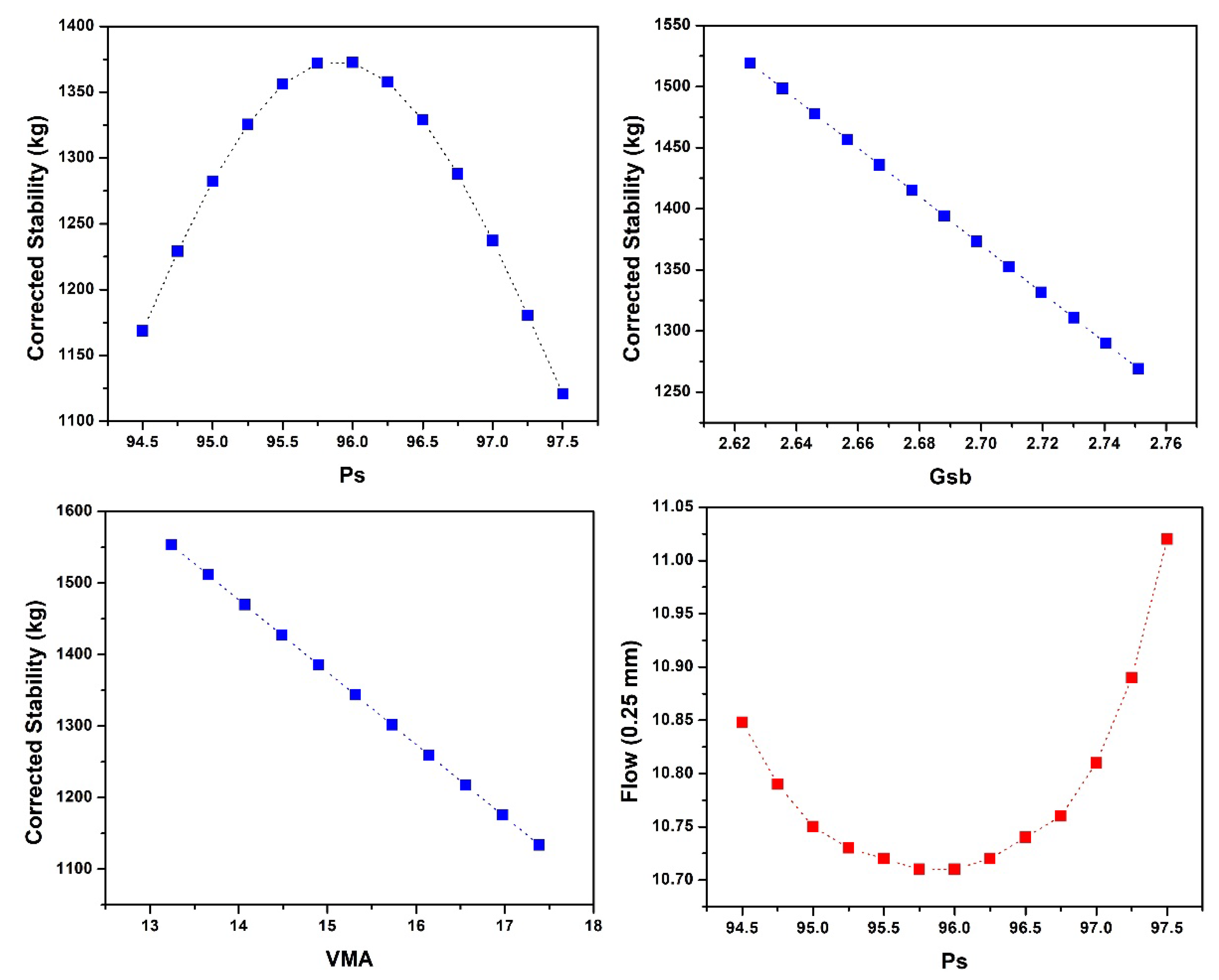
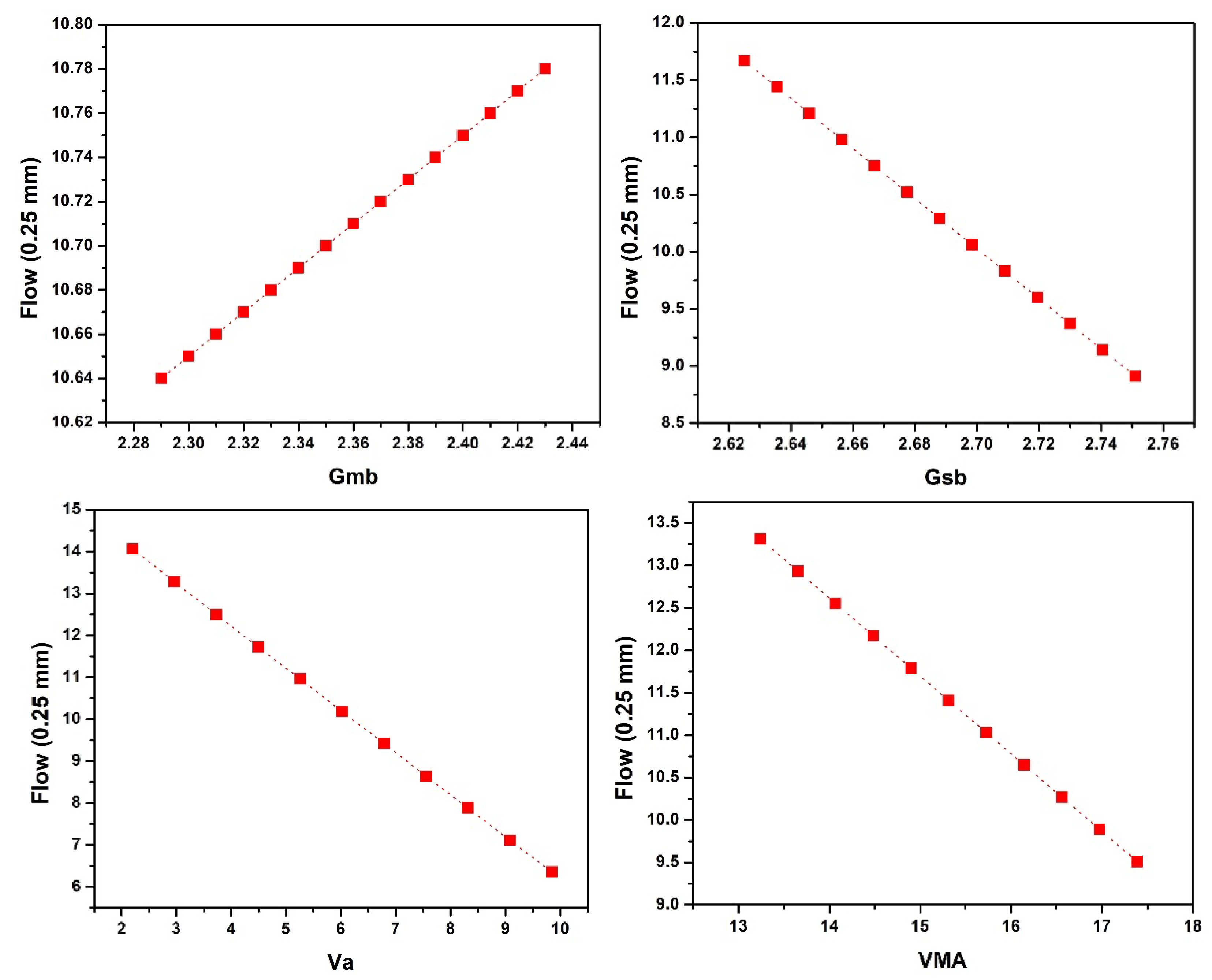
• According to the investigation on the influence of input parameters on MS and MF, it was concluded that with the increase in Ps, the MS first increases then drops, while MF first decreases and then rises. Downward linear trends were found for Gsb and VMA in the case of MS and Gsb, and Va and VMA in the case of MF. While in the case of MF, Gmb followed the upward linear trend.
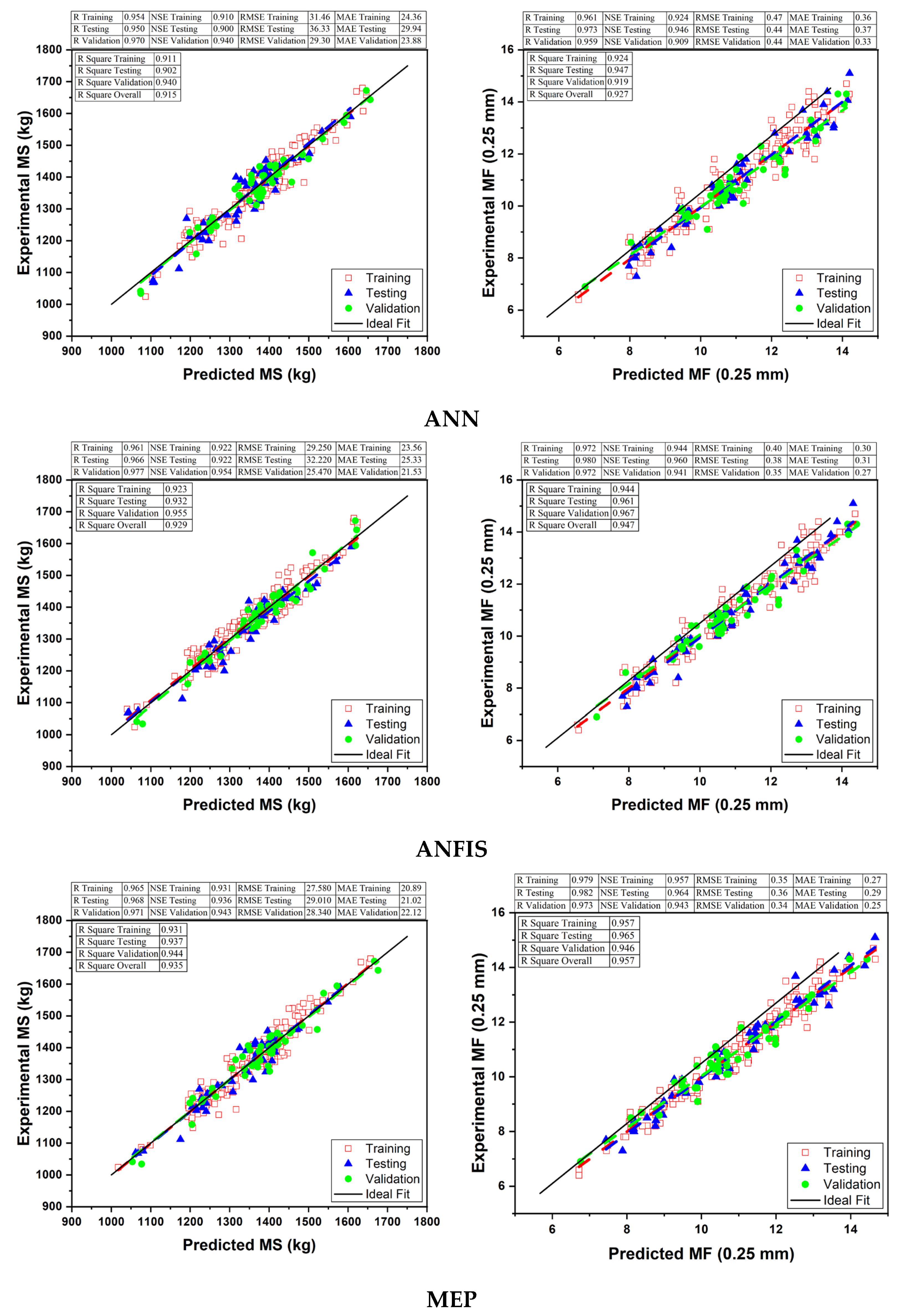
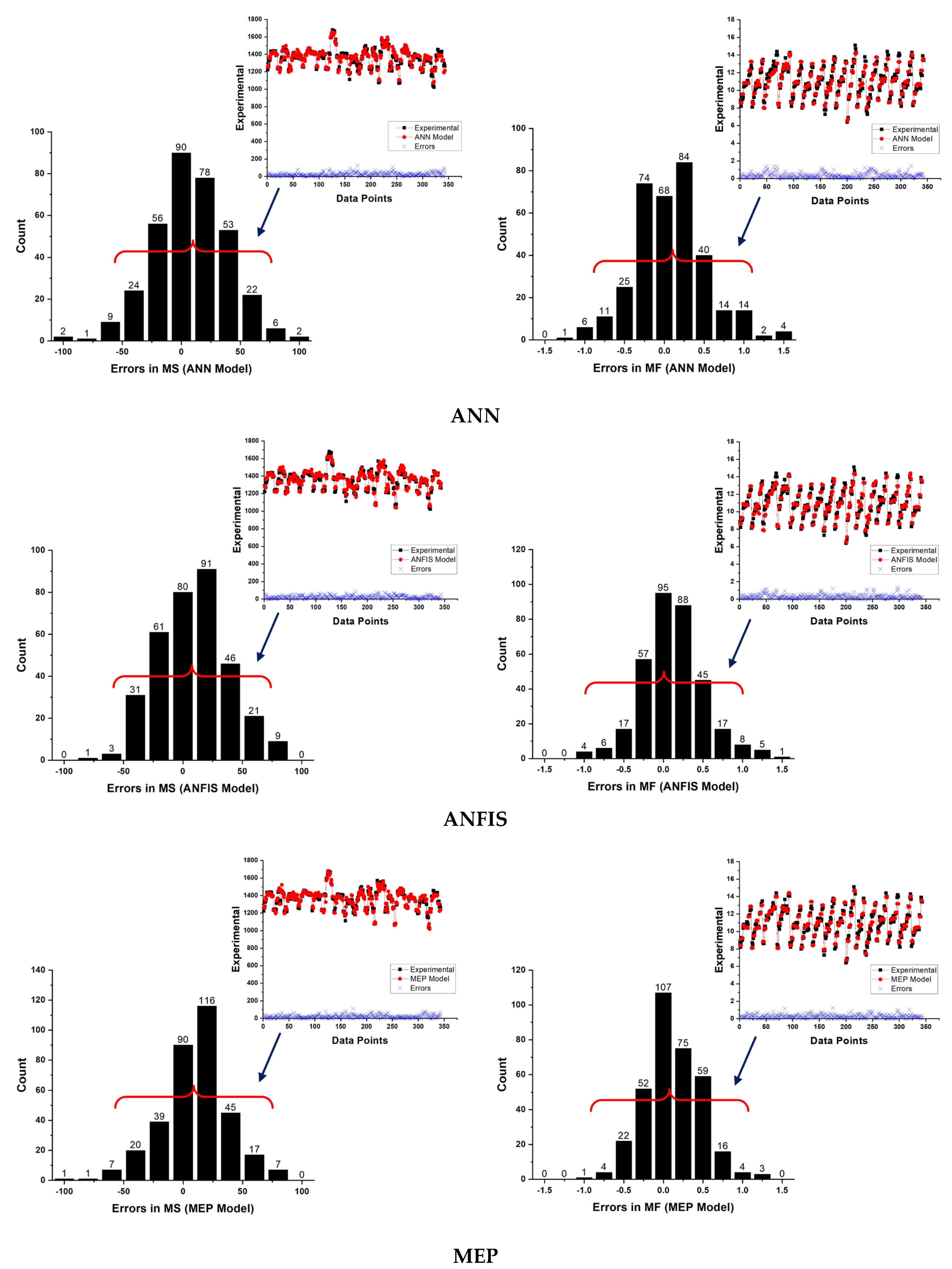
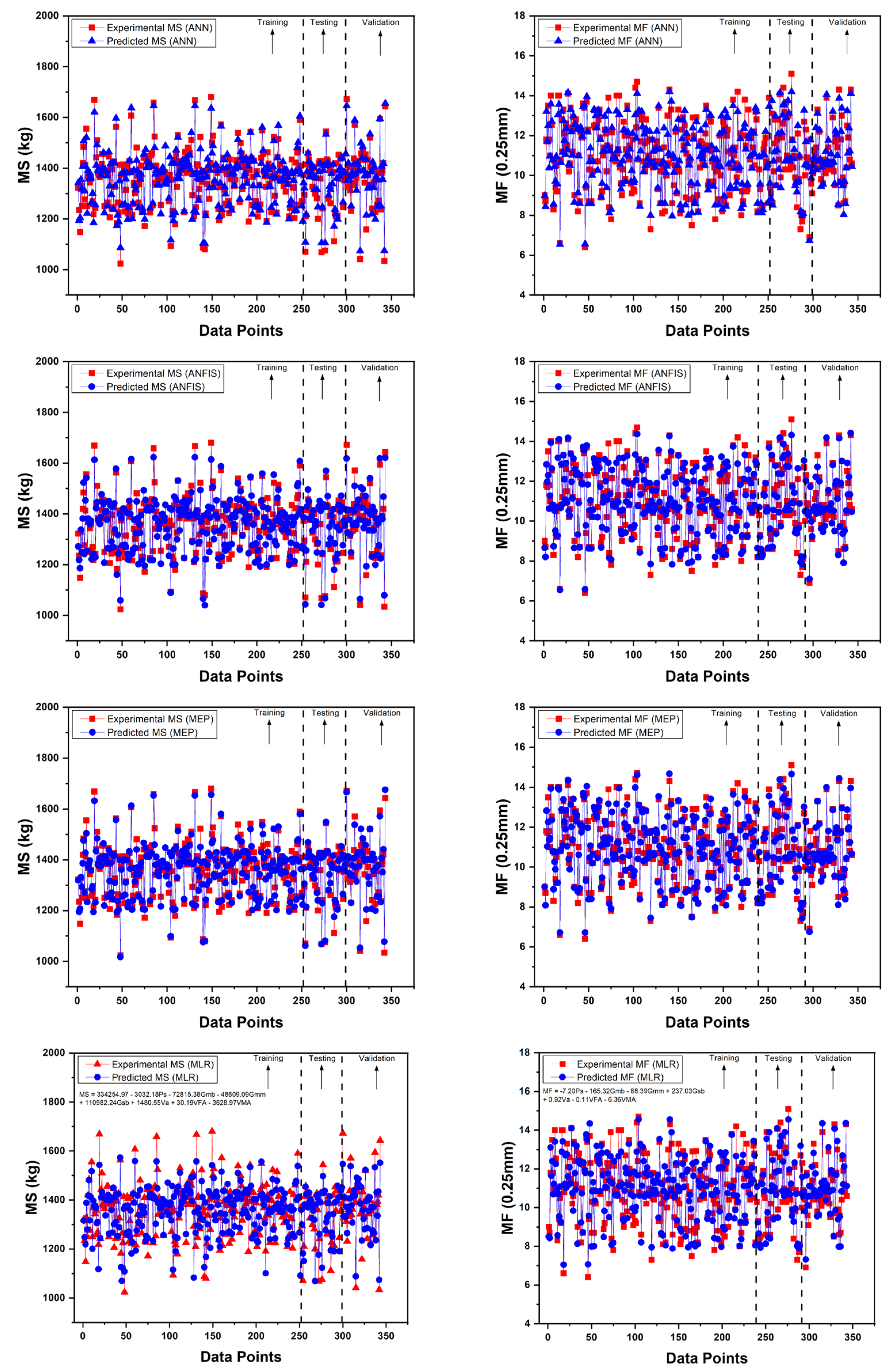
• Models based on ANN, ANFIS, and MEP have the ability to predict MS and MF with higher accuracy. Additionally, the MS and MF predicted while employing the MEP technique is better than ANN and ANFIS. The MEP approach simplifies the derivation of MS and MF while maintaining a reasonable level of accuracy between simulated and experimental data.
• To avoid the over-fitting of the employed approaches, i.e., ANN, ANFIS, and MEP, a variety of methods, including data division and preprocessing were utilized to minimize the complexity of the developed models. Sensitivity and parametric analysis were carried out, and are covered in length in the paper. The results of the parametric study were found to be inconsistent with the trends of previous research studies.
• All the models were evaluated using RSE, MAE, NSE, RMSE, RRMSE, R², and R. Overall, the comparison results show that all three approaches are effective and trustworthy for predicting the MS and MF of asphalt pavements; however, MEP technique outperformed ANN and ANFIS based on various statistical checks. MEP’s mathematical expressions (Equations (22) and (23)) are substantially simpler than the proposed models of ANN and ANFIS. The latter strategies, on the other hand, suffer from overfitting of data, NN’s limitations, and complexity in the network’s structure. It is suggested that the developed MEP models be used in everyday practice.
• The existing models can be used to estimate the MS and MF of asphalt pavements using basic geotechnical indices, which is an efficient, cost-effective, reliable, and time-saving solution to deal with the hectic and time-consuming process involved in the determination of MS and MF, leading to sustainable construction.

Ultimately, it is crucial to note that, based on the finding of this research study, AI techniques are extremely useful and robust tools for solving issues with complicated mechanisms, notably in the field of pavement engineering. The mathematical expressions can be intelligently generalized to previous data which is unseen. The authors also suggest that the outcomes of this research study be validated using other AI approaches, such as SVM, Ensemble Random Forest (ERF), and Gradient Boosted (GB). Because of their intrinsic flaws, such as model uncertainty, knowledge extraction, and interpretability, soft computing techniques are still facing opposition. To acquire a better understanding of the learning process, special emphasis must be made on gaining advanced knowledge about the hidden physical process, based on human expertise, or engineering judgement.

References

1. Miani, M.; Dunnhofer, M.; Rondinella, F.; Manthos, E.; Valentin, J.; Micheloni, C.; Baldo, N. Bituminous Mixtures Experimental Data Modeling Using a Hyperparameters-Optimized Machine Learning Approach. Appl. Sci. 2021, 11, 11710. [Google Scholar] [CrossRef]
2. Zhou, F.; Scullion, T.; Sun, L. Verification and modeling of three-stage permanent deformation behavior of asphalt mixes. J. Transp. Eng. 2004, 130, 486–494. [Google Scholar] [CrossRef]
3. Gandomi, A.H.; Alavi, A.H.; Mirzahosseini, M.R.; Nejad, F.M. Nonlinear genetic-based models for prediction of flow number of asphalt mixtures. J. Mater. Civ. Eng. 2011, 23, 248–263. [Google Scholar] [CrossRef]
4. Alavi, A.H.; Ameri, M.; Gandomi, A.H.; Mirzahosseini, M.R. Formulation of flow number of asphalt mixes using a hybrid computational method. Constr. Build. Mater. 2011, 25, 1338–1355. [Google Scholar] [CrossRef]
5. Dias, J.F.; Picado-Santos, L.; Capitão, S. Mechanical performance of dry process fine crumb rubber asphalt mixtures placed on the Portuguese road network. Constr. Build. Mater. 2014, 73, 247–254. [Google Scholar] [CrossRef]
6. Liu, Q.T.; Wu, S.P. Effects of steel wool distribution on properties of porous asphalt concrete. In Key Engineering Materials; Trans Tech Publications Ltd.: Zurich, Switzerland, 2014; pp. 150–154. [Google Scholar]
7. García, A.; Norambuena-Contreras, J.; Bueno, M.; Partl, M.N. Influence of Steel Wool Fibers on the Mechanical, Termal, and Healing Properties of Dense Asphalt Concrete; ASTM International: West Conshohocken, PN, USA, 2014. [Google Scholar]
8. Pasandín, A.; Pérez, I. Overview of bituminous mixtures made with recycled concrete aggregates. Constr. Build. Mater. 2015, 74, 151–161. [Google Scholar] [CrossRef] [Green Version]
9. Zaumanis, M.; Mallick, R.B.; Frank, R. 100% hot mix asphalt recycling: Challenges and benefits. Transp. Res. Procedia 2016, 14, 3493–3502. [Google Scholar] [CrossRef] [Green Version]
10. Wang, L.; Gong, H.; Hou, Y.; Shu, X.; Huang, B. Advances in pavement materials, design, characterisation, and simulation. Road Mater. Pavement Des. 2017, 18, 1–11. [Google Scholar] [CrossRef]
11. Erkens, S.; Liu, X.; Scarpas, A. 3D finite element model for asphalt concrete response simulation. Int. J. Geomech. 2002, 2, 305–330. [Google Scholar] [CrossRef]
12. Giunta, M.; Pisano, A.A. One-Dimensional Visco-Elastoplastic Constitutive Model for Asphalt Concrete. Multidiscip. Model. Mater. Struct. 2006, 2, 247–264. [Google Scholar] [CrossRef]
13. Underwood, S.B.; Kim, R.Y. Viscoelastoplastic continuum damage model for asphalt concrete in tension. J. Eng. Mech. 2011, 137, 732–739. [Google Scholar] [CrossRef]
14. Yun, T.; Richard Kim, Y. Viscoelastoplastic modeling of the behavior of hot mix asphalt in compression. KSCE J. Civ. Eng. 2013, 17, 1323–1332. [Google Scholar] [CrossRef]
15. Pasetto, M.; Baldo, N. Computational analysis of the creep behaviour of bituminous mixtures. Constr. Build. Mater. 2015, 94, 784–790. [Google Scholar] [CrossRef]
16. Di Benedetto, H.; Sauzéat, C.; Clec’h, P. Anisotropy of bituminous mixture in the linear viscoelastic domain. Mech. Time Depend. Mater. 2016, 20, 281–297. [Google Scholar] [CrossRef]
17. Pasetto, M.; Baldo, N. Numerical visco-elastoplastic constitutive modelization of creep recovery tests on hot mix asphalt. J. Traffic Transp. Eng. 2016, 3, 390–397. [Google Scholar] [CrossRef]
18. Darabi, M.K.; Huang, C.-W.; Bazzaz, M.; Masad, E.A.; Little, D.N. Characterization and validation of the nonlinear viscoelastic-viscoplastic with hardening-relaxation constitutive relationship for asphalt mixtures. Constr. Build. Mater. 2019, 216, 648–660. [Google Scholar] [CrossRef]
19. Anwar, M.K.; Shah, S.A.R.; Sadiq, A.N.; Siddiq, M.U.; Ahmad, H.; Nawaz, S.; Javead, A.; Saeed, M.H.; Khan, A.R. Symmetric performance analysis for mechanical properties of sustainable asphalt materials under varying temperature conditions: An application of DT and NDT digital techniques. Symmetry 2020, 12, 433. [Google Scholar] [CrossRef] [Green Version]
20. Arifuzzaman, M.; Aniq Gul, M.; Khan, K.; Hossain, S.Z. Application of artificial intelligence (ai) for sustainable highway and road system. Symmetry 2020, 13, 60. [Google Scholar] [CrossRef]
21. Kim, S.-H.; Kim, N. Development of performance prediction models in flexible pavement using regression analysis method. KSCE J. Civ. Eng. 2006, 10, 91–96. [Google Scholar] [CrossRef]
22. Laurinavičius, A.; Oginskas, R. Experimental research on the development of rutting in asphalt concrete pavements reinforced with geosynthetic materials. J. Civ. Eng. Manag. 2006, 12, 311–317. [Google Scholar] [CrossRef]
23. Shukla, P.K.; Das, A. A re-visit to the development of fatigue and rutting equations used for asphalt pavement design. Int. J. Pavement Eng. 2008, 9, 355–364. [Google Scholar] [CrossRef]
24. Rahman, A.A.; Mendez Larrain, M.M.; Tarefder, R.A. Development of a nonlinear rutting model for asphalt concrete based on Weibull parameters. Int. J. Pavement Eng. 2019, 20, 1055–1064. [Google Scholar] [CrossRef]
25. Zhang, W.; Zhang, R.; Wu, C.; Goh, A.T.C.; Lacasse, S.; Liu, Z.; Liu, H. State-of-the-art review of soft computing applications in underground excavations. Geosci. Front. 2020, 11, 1095–1106. [Google Scholar] [CrossRef]
26. Dobrescu, C. Dynamic Response of the Newton Voigt–Kelvin Modelled Linear Viscoelastic Systems at Harmonic Actions. Symmetry 2020, 12, 1571. [Google Scholar] [CrossRef]
27. Li, H.; Wu, A.; Wang, H. Evaluation of short-term strength development of cemented backfill with varying sulphide contents and the use of additives. J. Environ. Manag. 2019, 239, 279–286. [Google Scholar] [CrossRef]
28. Pham, B.T.; Tien Bui, D.; Dholakia, M.; Prakash, I.; Pham, H.V. A comparative study of least square support vector machines and multiclass alternating decision trees for spatial prediction of rainfall-induced landslides in a tropical cyclones area. Geotech. Geol. Eng. 2016, 34, 1807–1824. [Google Scholar] [CrossRef]
29. Gandomi, A.H.; Roke, D.A. Assessment of artificial neural network and genetic programming as predictive tools. Adv. Eng. Softw. 2015, 88, 63–72. [Google Scholar] [CrossRef]
30. Sathyapriya, S.; Arumairaj, P.; Ranjini, D. Prediction of unconfined compressive strength of a stabilised expansive clay soil using ANN and regression analysis (SPSS). Asian J. Res. Soc. Sci. Humanit. 2017, 7, 109–123. [Google Scholar] [CrossRef]
31. Alade, I.O.; Bagudu, A.; Oyehan, T.A.; Abd Rahman, M.A.; Saleh, T.A.; Olatunji, S.O. Estimating the refractive index of oxygenated and deoxygenated hemoglobin using genetic algorithm-support vector regression model. Comput. Methods Programs Biomed. 2018, 163, 135–142. [Google Scholar] [CrossRef]
32. Iqbal, M.F.; Liu, Q.-f.; Azim, I.; Zhu, X.; Yang, J.; Javed, M.F.; Rauf, M. Prediction of mechanical properties of green concrete incorporating waste foundry sand based on gene expression programming. J. Hazard. Mater. 2020, 384, 121322. [Google Scholar] [CrossRef]
33. Wu, Q.; Wu, B.; Hu, C.; Yan, X. Evolutionary Multilabel Classification Algorithm Based on Cultural Algorithm. Symmetry 2021, 13, 322. [Google Scholar] [CrossRef]
34. Shahin, M.A. Genetic programming for modelling of geotechnical engineering systems. In Handbook of Genetic Programming Applications; Springer: Berlin/Heidelberg, Germany, 2015; pp. 37–57. [Google Scholar]
35. Li, L.-L.; Liu, J.-Q.; Zhao, W.-B.; Dong, L. Fault Diagnosis of High-Speed Brushless Permanent-Magnet DC Motor Based on Support Vector Machine Optimized by Modified Grey Wolf Optimization Algorithm. Symmetry 2021, 13, 163. [Google Scholar] [CrossRef]
36. Çanakcı, H.; Baykasoğlu, A.; Güllü, H. Prediction of compressive and tensile strength of Gaziantep basalts via neural networks and gene expression programming. Neural Comput. Appl. 2009, 18, 1031–1041. [Google Scholar] [CrossRef]
37. Ozbek, A.; Unsal, M.; Dikec, A. Estimating uniaxial compressive strength of rocks using genetic expression programming. J. Rock Mech. Geotech. Eng. 2013, 5, 325–329. [Google Scholar] [CrossRef] [Green Version]
38. Khan, M.A.; Shah, M.I.; Javed, M.F.; Khan, M.I.; Rasheed, S.; El-Shorbagy, M.; El-Zahar, E.R.; Malik, M. Application of random forest for modelling of surface water salinity. Ain Shams Eng. J. 2022, 13, 101635. [Google Scholar] [CrossRef]
39. Das, S.K. 10 Artificial neural networks in geotechnical engineering: Modeling and application issues. Metaheuristics Water Geotech Transp. Eng. 2013, 45, 231–267. [Google Scholar]
40. Giustolisi, O.; Doglioni, A.; Savic, D.A.; Webb, B. A multi-model approach to analysis of environmental phenomena. Environ. Model. Softw. 2007, 22, 674–682. [Google Scholar] [CrossRef] [Green Version]
41. Shahin, M.A.; Jaksa, M.B.; Maier, H.R. Recent advances and future challenges for artificial neural systems in geotechnical engineering applications. Adv. Artif. Neural Syst. 2009, 2009, 308239. [Google Scholar] [CrossRef]
42. Mohammadzadeh, S.D.; Kazemi, S.-F.; Mosavi, A.; Nasseralshariati, E.; Tah, J.H. Prediction of compression index of fine-grained soils using a gene expression programming model. Infrastructures 2019, 4, 26. [Google Scholar] [CrossRef] [Green Version]
43. Zhang, Q.; Barri, K.; Jiao, P.; Salehi, H.; Alavi, A.H. Genetic programming in civil engineering: Advent, applications and future trends. Artif. Intell. Rev. 2021, 54, 1863–1885. [Google Scholar] [CrossRef]
44. Awan, H.H.; Hussain, A.; Javed, M.F.; Qiu, Y.; Alrowais, R.; Mohamed, A.M.; Fathi, D.; Alzahrani, A.M. Predicting Marshall Flow and Marshall Stability of Asphalt Pavements Using Multi Expression Programming. Buildings 2022, 12, 314. [Google Scholar] [CrossRef]
45. McCulloch, W.S.; Pitts, W. A logical calculus of the ideas immanent in nervous activity. Bull. Math. Biophys. 1943, 5, 115–133. [Google Scholar] [CrossRef]
46. Zacarias-Morales, N.; Pancardo, P.; Hernández-Nolasco, J.A.; Garcia-Constantino, M. Attention-inspired artificial neural networks for speech processing: A systematic review. Symmetry 2021, 13, 214. [Google Scholar] [CrossRef]
47. Shahin, M.A.; Jaksa, M.B.; Maier, H.R. Artificial neural network applications in geotechnical engineering. Aust. Geomech. 2001, 36, 49–62. [Google Scholar]
48. Yaman, M.A.; Abd Elaty, M.; Taman, M. Predicting the ingredients of self compacting concrete using artificial neural network. Alex. Eng. J. 2017, 56, 523–532. [Google Scholar] [CrossRef]
49. Jang, J.-S. ANFIS: Adaptive-network-based fuzzy inference system. IEEE Trans. Syst. Man Cybern. 1993, 23, 665–685. [Google Scholar] [CrossRef]
50. Sugeno, M. Industrial Applications of Fuzzy Control; Elsevier Science Inc.: Amsterdam, The Netherlands, 1985. [Google Scholar]
51. Mazari, M.; Rodriguez, D.D. Prediction of pavement roughness using a hybrid gene expression programming-neural network technique. J. Traffic Transp. Eng. 2016, 3, 448–455. [Google Scholar] [CrossRef] [Green Version]
52. Oltean, M.; Dumitrescu, D. Multi expression programming. J. Genet. Program. Evolvable Mach. 2002. Available online: https://www.researchgate.net/publication/2918165_Multi_Expression_Programming (accessed on 19 September 2022).
53. Baykasoğlu, A.; Güllü, H.; Çanakçı, H.; Özbakır, L. Prediction of compressive and tensile strength of limestone via genetic programming. Expert Syst. Appl. 2008, 35, 111–123. [Google Scholar] [CrossRef]
54. Alavi, A.H.; Gandomi, A.H.; Sahab, M.G.; Gandomi, M. Multi expression programming: A new approach to formulation of soil classification. Eng. Comput. 2010, 26, 111–118. [Google Scholar] [CrossRef]
55. Alavi, A.H.; Mollahasani, A.; Gandomi, A.H.; Bazaz, J.B. Formulation of secant and reloading soil deformation moduli using multi expression programming. Eng. Comput. 2012, 29, 173–197. [Google Scholar] [CrossRef]
56. Cabalar, A.F.; Cevik, A. Genetic programming-based attenuation relationship: An application of recent earthquakes in turkey. Comput. Geosci. 2009, 35, 1884–1896. [Google Scholar] [CrossRef]
57. Tapkın, S.; Çevik, A.; Uşar, Ü. Prediction of Marshall test results for polypropylene modified dense bituminous mixtures using neural networks. Expert Syst. Appl. 2010, 37, 4660–4670. [Google Scholar] [CrossRef]
58. Nguyen, H.-L.; Le, T.-H.; Pham, C.-T.; Le, T.-T.; Ho, L.S.; Le, V.M.; Pham, B.T.; Ly, H.-B. Development of hybrid artificial intelligence approaches and a support vector machine algorithm for predicting the marshall parameters of stone matrix asphalt. Appl. Sci. 2019, 9, 3172. [Google Scholar] [CrossRef] [Green Version]
59. Saffarzadeh, M.; Heidaripanah, A. Effect of asphalt content on the marshall stability of asphalt concrete using artificial neural networks. Sci. Iran. 2009, 16, 98–105. [Google Scholar]
60. Ozgan, E. Artificial neural network based modelling of the Marshall Stability of asphalt concrete. Expert Syst. Appl. 2011, 38, 6025–6030. [Google Scholar] [CrossRef]
61. Baldo, N.; Manthos, E.; Miani, M. Stiffness modulus and marshall parameters of hot mix asphalts: Laboratory data modeling by artificial neural networks characterized by cross-validation. Appl. Sci. 2019, 9, 3502. [Google Scholar] [CrossRef] [Green Version]
62. Shah, S.A.R.; Anwar, M.K.; Arshad, H.; Qurashi, M.A.; Nisar, A.; Khan, A.N.; Waseem, M. Marshall stability and flow analysis of asphalt concrete under progressive temperature conditions: An application of advance decision-making approach. Constr. Build. Mater. 2020, 262, 120756. [Google Scholar] [CrossRef]
63. Morova, N.; Sargin, Ş.; Terzi, S.; Saltan, M.; Serin, S. Modeling Marshall Stability of light asphalt concretes fabricated using expanded clay aggregate with Artificial Neural Networks. In Proceedings of the 2012 International Symposium on Innovations in Intelligent Systems and Applications, Trabzon, Turkey, 2–4 July 2012; pp. 1–4. [Google Scholar]
64. Morova, N.; Eriskin, E.; Terzi, S.; Karahancer, S.; Serin, S.; Saltan, M.; Usta, P. Modelling Marshall Stability of fiber reinforced asphalt mixtures with ANFIS. In Proceedings of the 2017 IEEE International Conference on INnovations in Intelligent SysTems and Applications (INISTA), Gdynia, Poland, 3–5 July 2017; pp. 174–179. [Google Scholar]
65. Serin, S.; Morova, N.; Sargın, Ş.; Terzi, S.; Saltan, M. Modeling Marshall stability of lightweight asphalt concretes fabricated using expanded clay aggregate with anfis. In Proceedings of the BCCCE—International Balkans Conference on Challenges of Civil Engineering, Epoka, Albania, 23–25 May 2013. [Google Scholar]
66. Mistry, R.; Roy, T.K. Predicting Marshall stability and flow of bituminous mix containing waste fillers by the adaptive neuro-fuzzy inference system. Rev. Construcción 2020, 19, 209–219. [Google Scholar] [CrossRef]
67. Fabani, M.P.; Capossio, J.P.; Román, M.C.; Zhu, W.; Rodriguez, R.; Mazza, G. Producing non-traditional flour from watermelon rind pomace: Artificial neural network (ANN) modeling of the drying process. J. Environ. Manag. 2021, 281, 111915. [Google Scholar] [CrossRef]
68. Venkatesh, K.; Bind, Y.K. ANN and neuro-fuzzy modeling for shear strength characterization of soils. Proc. Natl. Acad. Sci. USA 2020, 92, 243–249. [Google Scholar] [CrossRef]
69. Khan, M.A.; Aslam, F.; Javed, M.F.; Alabduljabbar, H.; Deifalla, A.F. New prediction models for the compressive strength and dry-thermal conductivity of bio-composites using novel machine learning algorithms. J. Clean. Prod. 2022, 350, 131364. [Google Scholar] [CrossRef]
70. Sada, S.; Ikpeseni, S. Evaluation of ANN and ANFIS modeling ability in the prediction of AISI 1050 steel machining performance. Heliyon 2021, 7, e06136. [Google Scholar] [CrossRef]
71. Kourgialas, N.N.; Dokou, Z.; Karatzas, G.P. Statistical analysis and ANN modeling for predicting hydrological extremes under climate change scenarios: The example of a small Mediterranean agro-watershed. J. Environ. Manag. 2015, 154, 86–101. [Google Scholar] [CrossRef] [PubMed]
72. Khan, M.A.; Zafar, A.; Farooq, F.; Javed, M.F.; Alyousef, R.; Alabduljabbar, H.; Khan, M.I. Geopolymer concrete compressive strength via artificial neural network, adaptive neuro fuzzy interface system, and gene expression programming with K-fold cross validation. Front. Mater. 2021, 8, 621163. [Google Scholar] [CrossRef]
73. Koçak, Y.; Şiray, G.Ü. New activation functions for single layer feedforward neural network. Expert Syst. Appl. 2021, 164, 113977. [Google Scholar] [CrossRef]
74. Cai, C.; Xu, Y.; Ke, D.; Su, K. Deep neural networks with multistate activation functions. Comput. Intell. Neurosci. 2015, 2015, 721367. [Google Scholar] [CrossRef] [Green Version]
75. Tang, C.; Luktarhan, N.; Zhao, Y. SAAE-DNN: Deep Learning Method on Intrusion Detection. Symmetry 2020, 12, 1695. [Google Scholar] [CrossRef]
76. Ramachandran, P.; Zoph, B.; Le, Q. Searching for Activation Functions. arXiv 2017, arXiv:1710.05941. [Google Scholar]
77. Xu, B.; Huang, R.; Li, M. Revise saturated activation functions. arXiv 2016, arXiv:1602.05980. [Google Scholar]
78. Naresh Babu, K.; Edla, D.R. New algebraic activation function for multi-layered feed forward neural networks. IETE J. Res. 2017, 63, 71–79. [Google Scholar] [CrossRef]
79. Malinov, S.; Sha, W.; McKeown, J. Modelling the correlation between processing parameters and properties in titanium alloys using artificial neural network. Comput. Mater. Sci. 2001, 21, 375–394. [Google Scholar] [CrossRef] [Green Version]
80. Tahani, M.; Vakili, M.; Khosrojerdi, S. Experimental evaluation and ANN modeling of thermal conductivity of graphene oxide nanoplatelets/deionized water nanofluid. Int. Commun. Heat Mass Transf. 2016, 76, 358–365. [Google Scholar] [CrossRef]
81. Tang, Y.-J.; Zhang, Q.-Y.; Lin, W. Artificial neural network based spectrum sensing method for cognitive radio. In Proceedings of the 2010 6th International Conference on Wireless Communications Networking and Mobile Computing (WiCOM), Shenzhen, China, 23–25 September 2010; pp. 1–4. [Google Scholar]
82. Dorofki, M.; Elshafie, A.H.; Jaafar, O.; Karim, O.A.; Mastura, S. Comparison of artificial neural network transfer functions abilities to simulate extreme runoff data. Int. Proc. Chem. Biol. Environ. Eng. 2012, 33, 39–44. [Google Scholar]
83. Hanandeh, S.; Ardah, A.; Abu-Farsakh, M. Using artificial neural network and genetics algorithm to estimate the resilient modulus for stabilized subgrade and propose new empirical formula. Transp. Geotech. 2020, 24, 100358. [Google Scholar] [CrossRef]
84. Alavi, A.H.; Gandomi, A.H. A robust data mining approach for formulation of geotechnical engineering systems. Eng. Comput. 2011, 28, 242–274. [Google Scholar] [CrossRef]
85. Nosratabadi, S.; Mosavi, A.; Duan, P.; Ghamisi, P.; Filip, F.; Band, S.S.; Reuter, U.; Gama, J.; Gandomi, A.H. Data science in economics: Comprehensive review of advanced machine learning and deep learning methods. Mathematics 2020, 8, 1799. [Google Scholar] [CrossRef]
86. Shahin, M.A. Artificial intelligence in geotechnical engineering: Applications, modeling aspects, and future directions. In Metaheuristics in Water, Geotechnical and Transport Engineering; Elsevier: Amsterdam, The Netherlands, 2013; pp. 169–204. [Google Scholar]
87. Sperotto, A.; Molina, J.-L.; Torresan, S.; Critto, A.; Marcomini, A. Reviewing Bayesian Networks potentials for climate change impacts assessment and management: A multi-risk perspective. J. Environ. Manag. 2017, 202, 320–331. [Google Scholar] [CrossRef]
88. Khan, K.; Ashfaq, M.; Iqbal, M.; Khan, M.A.; Amin, M.N.; Shalabi, F.I.; Faraz, M.I.; Jalal, F.E. Multi Expression Programming Model for Strength Prediction of Fly-Ash-Treated Alkali-Contaminated Soils. Materials 2022, 15, 4025. [Google Scholar] [CrossRef]
89. Akan, R.; Keskin, S.N. The effect of data size of ANFIS and MLR models on prediction of unconfined compression strength of clayey soils. SN Appl. Sci. 2019, 1, 843. [Google Scholar] [CrossRef] [Green Version]
90. Golafshani, E.M.; Behnood, A.; Arashpour, M. Predicting the compressive strength of normal and High-Performance Concretes using ANN and ANFIS hybridized with Grey Wolf Optimizer. Constr. Build. Mater. 2020, 232, 117266. [Google Scholar] [CrossRef]
91. Sadeghizadeh, A.; Ebrahimi, F.; Heydari, M.; Tahmasebikohyani, M.; Ebrahimi, F.; Sadeghizadeh, A. Adsorptive removal of Pb (II) by means of hydroxyapatite/chitosan nanocomposite hybrid nanoadsorbent: ANFIS modeling and experimental study. J. Environ. Manag. 2019, 232, 342–353. [Google Scholar] [CrossRef] [PubMed]
92. Khan, K.; Jalal, F.E.; Khan, M.A.; Salami, B.A.; Amin, M.N.; Alabdullah, A.A.; Samiullah, Q.; Arab, A.M.A.; Faraz, M.I.; Iqbal, M. Prediction Models for Evaluating Resilient Modulus of Stabilized Aggregate Bases in Wet and Dry Alternating Environments: ANN and GEP Approaches. Materials 2022, 15, 4386. [Google Scholar] [CrossRef] [PubMed]
93. Islam, M.; Jaafar, W.Z.W.; Hin, L.S.; Osman, N.; Hossain, A.; Mohd, N.S. Development of an intelligent system based on ANFIS model for predicting soil erosion. Environ. Earth Sci. 2018, 77, 186. [Google Scholar] [CrossRef]
94. Khan, S.; Ali Khan, M.; Zafar, A.; Javed, M.F.; Aslam, F.; Musarat, M.A.; Vatin, N.I. Predicting the ultimate axial capacity of uniaxially loaded cfst columns using multiphysics artificial intelligence. Materials 2021, 15, 39. [Google Scholar] [CrossRef]
95. Goldberg, D.E. Genetic Algorithms in Search, Optimization, and Machine Learning; Addison-Wesley Longman Publishing Co., Inc.: Boston, MA, USA, 1989. [Google Scholar]
96. Koza, J.R. Genetic Programming: On the Programming of Computers by Means of Natural Selection; MIT Press: Cambridge, MA, USA, 1992; Volume 1. [Google Scholar]
97. Khan, M.A.; Memon, S.A.; Farooq, F.; Javed, M.F.; Aslam, F.; Alyousef, R. Compressive strength of fly-ash-based geopolymer concrete by gene expression programming and random forest. Adv. Civ. Eng. 2021, 2021, 6618407. [Google Scholar] [CrossRef]
98. Javed, M.F.; Farooq, F.; Memon, S.A.; Akbar, A.; Khan, M.A.; Aslam, F.; Alyousef, R.; Alabduljabbar, H.; Rehman, S.K.U. New prediction model for the ultimate axial capacity of concrete-filled steel tubes: An evolutionary approach. Crystals 2020, 10, 741. [Google Scholar] [CrossRef]
99. Alavi, A.H.; Gandomi, A.H.; Nejad, H.C.; Mollahasani, A.; Rashed, A. Design equations for prediction of pressuremeter soil deformation moduli utilizing expression programming systems. Neural Comput. Appl. 2013, 23, 1771–1786. [Google Scholar] [CrossRef]
100. Cheng, Z.-L.; Zhou, W.-H.; Garg, A. Genetic programming model for estimating soil suction in shallow soil layers in the vicinity of a tree. Eng. Geol. 2020, 268, 105506. [Google Scholar] [CrossRef]
101. Wang, H.-L.; Yin, Z.-Y. High performance prediction of soil compaction parameters using multi expression programming. Eng. Geol. 2020, 276, 105758. [Google Scholar] [CrossRef]
102. Chu, H.-H.; Khan, M.A.; Javed, M.; Zafar, A.; Khan, M.I.; Alabduljabbar, H.; Qayyum, S. Sustainable use of fly-ash: Use of gene-expression programming (GEP) and multi-expression programming (MEP) for forecasting the compressive strength geopolymer concrete. Ain Shams Eng. J. 2021, 12, 3603–3617. [Google Scholar] [CrossRef]
103. Khan, M.A.; Farooq, F.; Javed, M.F.; Zafar, A.; Ostrowski, K.A.; Aslam, F.; Malazdrewicz, S.; Maślak, M. Simulation of depth of wear of eco-friendly concrete using machine learning based computational approaches. Materials 2021, 15, 58. [Google Scholar] [CrossRef] [PubMed]
104. Aldrees, A.; Khan, M.A.; Tariq, M.A.U.R.; Mustafa Mohamed, A.; Ng, A.W.M.; Bakheit Taha, A.T. Multi-Expression Programming (MEP): Water Quality Assessment Using Water Quality Indices. Water 2022, 14, 947. [Google Scholar] [CrossRef]
105. Oltean, M.; Grosan, C. A comparison of several linear genetic programming techniques. Complex Syst. 2003, 14, 285–314. [Google Scholar]
106. Maeda, T. How to Rationally Compare the Performances of Different Machine Learning Models? PeerJ Prepr. 2018, 6, 2167–9843. [Google Scholar]
107. Abunama, T.; Othman, F.; Ansari, M.; El-Shafie, A. Leachate generation rate modeling using artificial intelligence algorithms aided by input optimization method for an MSW landfill. Environ. Sci. Pollut. Res. 2019, 26, 3368–3381. [Google Scholar] [CrossRef]
108. Shah, M.I.; Javed, M.F.; Abunama, T. Proposed formulation of surface water quality and modelling using gene expression, machine learning, and regression techniques. Environ. Sci. Pollut. Res. 2021, 28, 13202–13220. [Google Scholar] [CrossRef]
109. Papadimitriou, F. What is Spatial Complexity? In Spatial Complexity; Springer: Berlin/Heidelberg, Germany, 2020; pp. 3–18. [Google Scholar]
110. Papadimitriou, F. The Probabilistic Basis of Spatial Complexity. In Spatial Complexity; Springer: Berlin/Heidelberg, Germany, 2020; pp. 51–61. [Google Scholar]
111. Papadimitriou, F. Modelling spatial landscape complexity using the Levenshtein algorithm. Ecol. Inform. 2009, 4, 48–55. [Google Scholar] [CrossRef]
112. Rekha, M. MLmuse: Correlation and Collinearity—How They Can Make or Break a Model. Correlation Analysis and Collinearity|Data Science|Multicollinearity|Clairvoyant Blog (clairvoyantsoft.com). 2019. Available online: https://blog.clairvoyantsoft.com/correlation-and-collinearity-how-they-can-make-or-break-a-model-9135fbe6936a (accessed on 11 June 2022).
113. Shrestha, N. Detecting multicollinearity in regression analysis. Am. J. Appl. Math. Stat. 2020, 8, 39–42. [Google Scholar] [CrossRef]
114. Kim, J.H. Multicollinearity and misleading statistical results. Korean J. Anesthesiol. 2019, 72, 558–569. [Google Scholar] [CrossRef] [Green Version]
115. Al-Jamimi, H.A.; Bagudu, A.; Saleh, T.A. An intelligent approach for the modeling and experimental optimization of molecular hydrodesulfurization over AlMoCoBi catalyst. J. Mol. Liq. 2019, 278, 376–384. [Google Scholar] [CrossRef]
116. Alawi, M.; Rajab, M. Determination of optimum bitumen content and Marshall stability using neural networks for asphaltic concrete mixtures. In Proceedings of the 9th WSEAS International Conference on Computers, World Scientific and Engineering Academy and Society (WSEAS), Athens, Greece, 11–13 July 2005. [Google Scholar]
117. Kandil, K.A. Modeling marshall stability and flow for hot mix asphalt using artificial intelligence techniques. Nat. Sci. 2013, 11, 106–112. [Google Scholar]
118. Ogundipe, O.M. Marshall stability and flow of lime-modified asphalt concrete. Transp. Res. Procedia 2016, 14, 685–693. [Google Scholar] [CrossRef] [Green Version]
119. Mozumder, R.A.; Laskar, A.I. Prediction of unconfined compressive strength of geopolymer stabilized clayey soil using artificial neural network. Comput. Geotech. 2015, 69, 291–300. [Google Scholar] [CrossRef]
120. Jalal, M.; Grasley, Z.; Nassir, N.; Jalal, H. RETRACTED: Strength and dynamic elasticity modulus of rubberized concrete designed with ANFIS modeling and ultrasonic technique. Constr. Build. Mater. 2020, 240, 117920. [Google Scholar] [CrossRef]
121. Alade, I.O.; Abd Rahman, M.A.; Saleh, T.A. Predicting the specific heat capacity of alumina/ethylene glycol nanofluids using support vector regression model optimized with Bayesian algorithm. Sol. Energy 2019, 183, 74–82. [Google Scholar] [CrossRef]
122. Alade, I.O.; Abd Rahman, M.A.; Saleh, T.A. Modeling and prediction of the specific heat capacity of Al2O3/water nanofluids using hybrid genetic algorithm/support vector regression model. Nano Struct. Nano Objects 2019, 17, 103–111. [Google Scholar] [CrossRef]
123. Kisi, O.; Shiri, J.; Tombul, M. Modeling rainfall-runoff process using soft computing techniques. Comput. Geosci. 2013, 51, 108–117. [Google Scholar] [CrossRef]
124. Shahin, M.A. Use of evolutionary computing for modelling some complex problems in geotechnical engineering. Geomech. Geoengin. 2015, 10, 109–125. [Google Scholar] [CrossRef] [Green Version]
125. Emamgholizadeh, S.; Bahman, K.; Bateni, S.M.; Ghorbani, H.; Marofpoor, I.; Nielson, J.R. Estimation of soil dispersivity using soft computing approaches. Neural Comput. Appl. 2017, 28, 207–216. [Google Scholar] [CrossRef]
126. Aslam, F.; Elkotb, M.A.; Iqtidar, A.; Khan, M.A.; Javed, M.F.; Usanova, K.I.; Khan, M.I.; Alamri, S.; Musarat, M.A. Compressive strength prediction of rice husk ash using multiphysics genetic expression programming. Ain Shams Eng. J. 2022, 13, 101593. [Google Scholar] [CrossRef]
127. Erzin, Y. Artificial neural networks approach for swell pressure versus soil suction behaviour. Can. Geotech. J. 2007, 44, 1215–1223. [Google Scholar] [CrossRef]
128. Frank, I.E.; Todeschini, R. The Data Analysis Handbook; Elsevier: Amsterdam, The Netherlands, 1994. [Google Scholar]
129. Dao, D.V.; Ly, H.-B.; Trinh, S.H.; Le, T.-T.; Pham, B.T. Artificial intelligence approaches for prediction of compressive strength of geopolymer concrete. Materials 2019, 12, 983. [Google Scholar] [CrossRef] [Green Version]
130. Roy, P.P.; Roy, K. On some aspects of variable selection for partial least squares regression models. QSAR Comb. Sci. 2008, 27, 302–313. [Google Scholar] [CrossRef]
131. Iqbal, M.F.; Javed, M.F.; Rauf, M.; Azim, I.; Ashraf, M.; Yang, J.; Liu, Q.-f. Sustainable utilization of foundry waste: Forecasting mechanical properties of foundry sand based concrete using multi-expression programming. Sci. Total Environ. 2021, 780, 146524. [Google Scholar] [CrossRef]
132. Trucchia, A.; Frunzo, L. Surrogate based Global Sensitivity Analysis of ADM1-based Anaerobic Digestion Model. J. Environ. Manag. 2021, 282, 111456. [Google Scholar] [CrossRef]
133. Derbel, M.; Hachicha, W.; Aljuaid, A.M. Sensitivity Analysis of the Optimal Inventory-Pooling Strategies According to Multivariate Demand Dependence. Symmetry 2021, 13, 328. [Google Scholar] [CrossRef]
134. Khan, M.A.; Zafar, A.; Akbar, A.; Javed, M.F.; Mosavi, A. Application of Gene Expression Programming (GEP) for the prediction of compressive strength of geopolymer concrete. Materials 2021, 14, 1106. [Google Scholar] [CrossRef]
Figure 1. Architecture of (a) ANN, (b) ANFIS, and (c) MEP.
Symmetry 14 02324 g001aSymmetry 14 02324 g001b
Figure 2. Comparison of Predicted and Actual Values.
Symmetry 14 02324 g002
Figure 3. Comparison of Error Histograms for MS and MF.
Symmetry 14 02324 g003
Figure 4. Comparison of the Proposed Models for MS and MF using ANN, ANFIS, MEP, and MLR.
Symmetry 14 02324 g004
Figure 5. Results of SA Regarding Input Parameters.
Symmetry 14 02324 g005
Figure 6. Results of PA for MS and MF using MEP.
Symmetry 14 02324 g006aSymmetry 14 02324 g006b