Monitoring Dropping Densities with Unmanned Aerial Vehicles (UAV): An Effective Tool to Assess Distribution Patterns in Field Utilization by Foraging Geese

Abstract

Counting of droppings is often, with great effect, used as an indirect method to monitor the appearance and usage of an area by a population covering longer time spans. However, manual detecting and counting of droppings can be time-consuming and tedious, and with a risk of resulting in course estimations. In this context, we studied the use of imaging from unmanned aerial vehicles (UAVs) as a novel and enhanced tool to estimate the dropping densities and distributions of field foraging Arctic migratory geese, such as pink-footed goose Anser brachyrhynchus and barnacle goose Branta leucopsis. Aided by analysis in geographical information systems (GIS), we sought to detect and use fine-scale changes in the within-field dropping densities to evaluate avoidance distance to selected landscape elements. Data in the form of aerial photos from farmed grassland and pastures were collected in areas adjacent to Limfjorden, Northern Jutland, Denmark. The UAV proved usable for detecting droppings from field foraging geese, but with the applied UAV technology only at a low flying altitude (≤3 m), which rendered traditional methods for georeferencing inapplicable. A revised protocol for georeferencing of single aerial photos triggered from low altitudes was successfully developed, which was considered suitable for future use. Analyses based on the performed UAV data sampling allowed for an unprecedented fine-scale estimation of distribution patterns of the goose droppings and further for determination of optimal sampling frequencies (≤12 × 12 m spacing between photo samples) for calculation of density patterns, which reflected differences in foraging activity of geese across whole fields. Contagious dispersions in dropping densities were detected in the majority of fields indicating local, within-field displacements of the geese, which were illustrated by interpolated heatmaps. Additionally, avoidance distances were assessed for four landscape elements and detected with consistent results for windbreaks (100 m), roads (175 m) and wind turbines (1100 m) throughout the ten surveyed fields.

1. Introduction

A substantial conservational concern is the increasing number and sizes of landscape elements, often anthropogenic in character, such as wind turbines and roads [1,2]. The placement of such elements often coincides with farmland in close proximity to nature-protected wetlands, which constitute important feeding grounds for staging migratory geese [3,4]. These elements may cause the geese to alter behaviour and create possible barrier zones around the anthropogenic structures avoided by the foraging geese, which may decrease the field utilisation and cause displacement effects, ultimately reducing the carrying capacity of the areas [3,5,6].

Denmark internationally plays an important role as a stopover site and wintering ground for several Arctic migratory populations of geese, accommodating at times up to 70% of the Svalbard population of pink-footed geese (Anser brachyrhynchus) and up to 20% of the Baltic population of barnacle geese (Branta leucopsis) [2,7]. With this follows a responsibility for monitoring and implementing appropriate conservation planning and strategies to mitigate possible conflicts between geese and human interests, and simultaneously ensure suitable stopover sites and feeding grounds to sustain the populations during the non-breeding season [3,8].

Different methods have been developed for monitoring and analysing the distribution and trends in bird populations with the aim of optimising the accuracy and usability of the collected data [9,10]. With respect to migratory waterfowl species, such as geese, the methods applied include direct visual observations of birds, either by optical means from the ground [11,12], manned aircraft [13,14] or, more recently, by unmanned aerial vehicle (UAV) imaging [6,15,16,17,18]. Another approach is the more indirect method of manual counts of bird dropping densities, which enables monitoring of the activity of a population covering a longer timespan [4,19].

Ground counts with telescopic optics or counts with a laser rangefinder are used to gather reliable information on the relative position of individual geese at a given point in time [20]. The drawbacks of this method are a high workload, and for laser rangefinders, the resulting data often include only a few individuals out of a flock of many [20,21]. Manned aerial counts are typically more accurate but are costly and pose substantial personal risks of accidents [22,23]. More recently, aerial photos obtained by UAV imaging of the foraging geese have been explored, which give precise data on the exact location of all the birds contained in a flock and typically yield a higher number of birds in comparison to ground counts [24,25,26,27]. Further, monitoring with UAVs is often less costly and generally reduces the hours spent working in the field [28,29]. Together with the development of improved geographical information systems (GIS), UAV imaging techniques and software development create new, game-changing opportunities to assess and improve wildlife monitoring [23,30,31,32]. However, as with manual ground counts, the drawbacks of UAV imaging are that the method only gives data on the actual and momentary position of the individual geese at a given point in time in the field. Additionally, the method poses the risk of disturbing the birds [23,33,34]. Counteracting these mentioned drawbacks, gathering information on dropping densities gives the ability to estimate the foraging activity of all birds occurring over a longer timespan throughout the field and with a minimal risk of disturbing the birds. The dropping count method is suitable to estimate the distribution of geese, as they are herbivores and produce droppings at short time intervals (of about 5 min) during feeding and, further, they feed on open areas with typically low vegetation [19,26,35]. This renders the detection of droppings possible with a timespan of 3–4 weeks before disintegration in conditions with intermittent precipitation, such as in Denmark [4]. However, the conventional process of sampling dropping densities in transects in the field is labour intensive, time-consuming and, further, is typically only performed at low sampling frequencies, with the resulting risk of uncertain detection of dropping densities.

The aim of this study was to explore and evaluate a novel approach to gathering information on field utilization of foraging geese by using UAV imaging in combination with an optimized GIS-based workflow to measure dropping density in the field. By applying UAV imaging, it was possible to reduce the time needed for both the collection and georeferencing of the droppings. Furthermore, using UAV imaging would allow for information on the dropping density and goose distribution in the field to be gathered, covering a longer foraging time span than possible with direct observations of the geese by either a manual ground count or UAV imaging. In the present study, we investigated (i) if it was possible to detect droppings from foraging geese by UAV imaging of farmland pastures and at which flight heights, (ii) whether it was possible to georeference UAV photos of detectable droppings, and (iii) to find an optimal spatial positioning and sampling frequency for the aerial photos, thereby enabling fine-scale estimation of distribution patterns in farmland fields. Finally, (iv) we investigated if dropping densities obtained with UAV can allow for fine-scale evaluation of avoidance distances to landscape elements.

2. Materials and Methods

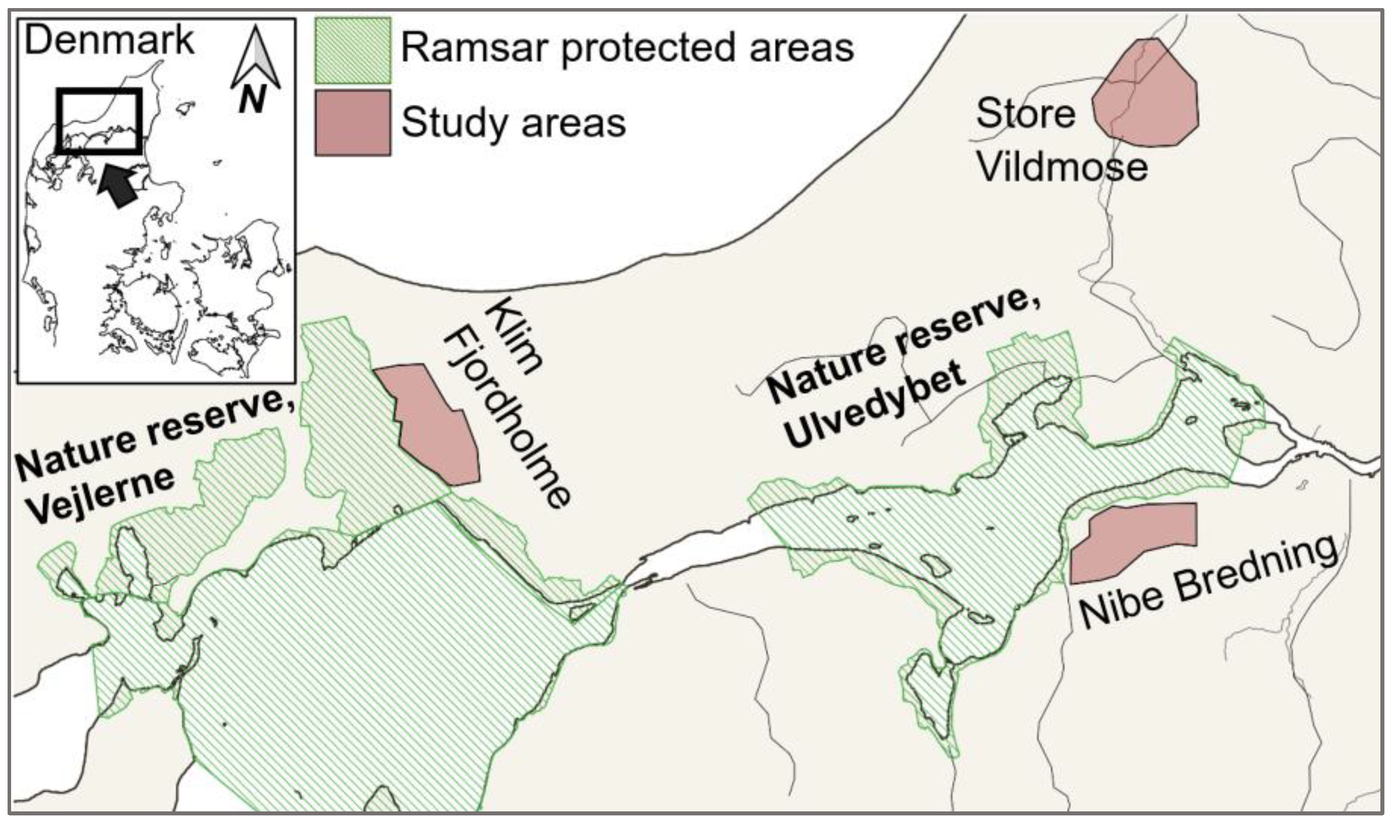
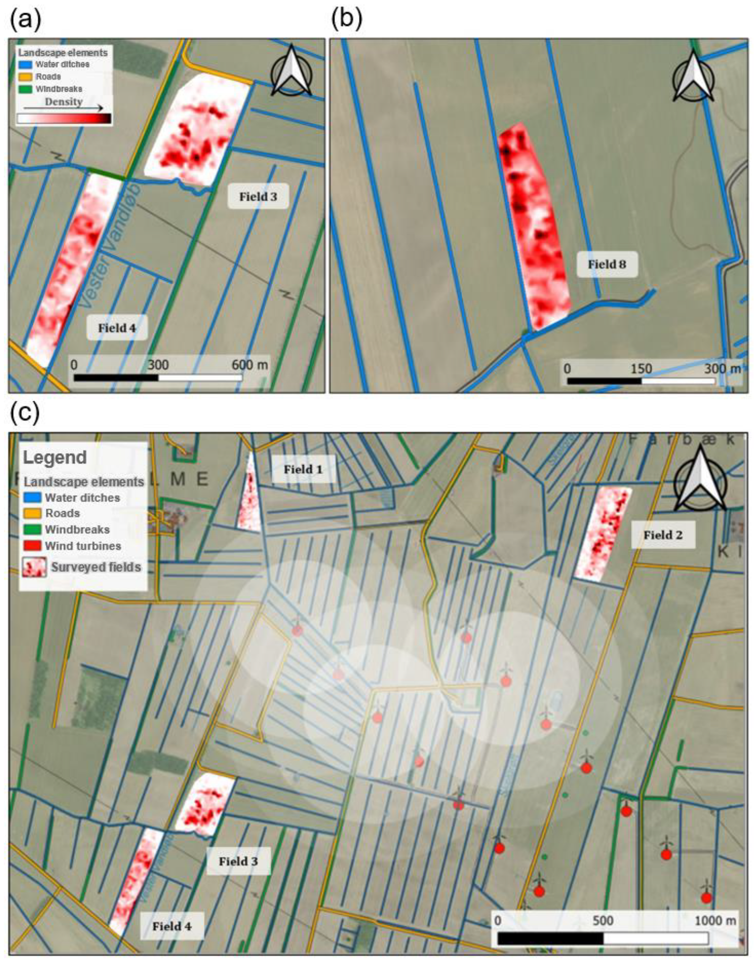
2.1. Study Area

Data were collected from 10 March to 18 April 2019 within three areas in northern Jutland, Denmark (Figure 1): Klim Fjordholme (57°04′40.8″ N 9°07′11.9″ E), Nibe Bredning (57°00′50.4″ N 9°43′39.7″ E) and Store Vildmose (57°14′22.3″ N 9°44′30.1″ E). During this period, the two focus species of the study, pink-footed goose (Anser brachyrhynchus) and barnacle goose (Branta leucopsis), still frequented the area on a regular basis before migrating north [8] and the weather allowed for longer consecutive dry field periods. The collecting areas were all important and regularly used as foraging areas for the spring staging geese and were located adjacent to wetland areas protected by the Ramsar convention, Vejlerne, Ulvedybet and Nibe Bredning [36,37,38]. Ten specific fields from these candidate areas, varying from 2.8–15.2 hectares (in total 58 ha), were chosen, which had the characteristics of cultivated grassland or pastures, allowing for the collection of data.

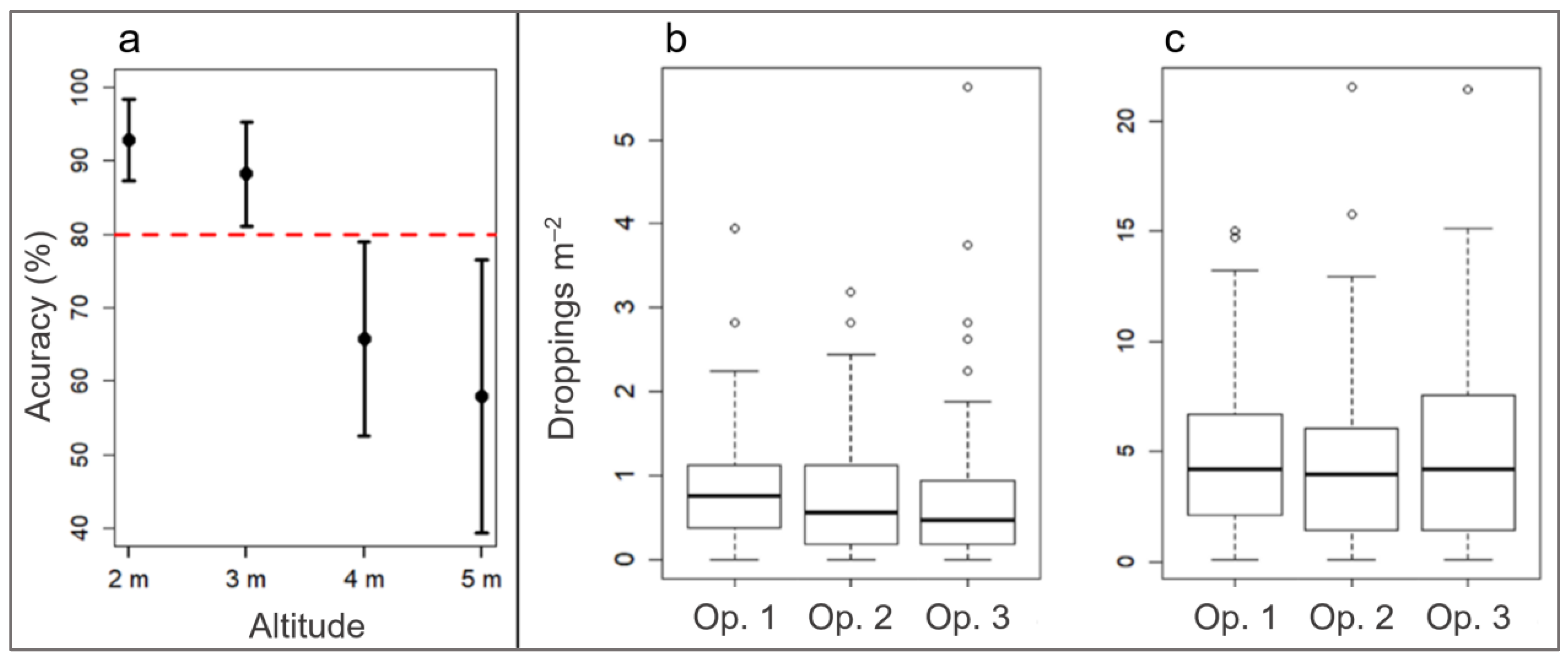
2.2. Maximum Flying Altitude

All aerial photos of goose droppings were collected using two similar consumer-grade UAVs, DJI Phantom 4 Pro and DJI Phantom 3 Pro Quadcopter (DJI Technology Co. Ltd., Shenzhen, China) [39], both of which are popular platforms for monitoring purposes [40,41]. Prior to data collection, the possibility of detecting and accuracy of counting droppings were tested by flying over a randomly chosen test field within the study area. Early in the study period, flights at altitudes of 5–10 m were performed but failed to produce useable results with respect to acceptable accuracy of dropping counts. A regular test of the maximum flying altitude was hence confined to the interval of altitudes between 2–5 m (Figure S1a,b). The UAV was flown over randomly placed visible circles of 40 cm in radius (0.53 m²). The number of droppings inside these circles was manually counted from the ground, and then photos were shot with the UAV at altitudes every meter from 2–5 m above the circles. For each altitude, 15 circle replicates were made. The visible number of droppings on all UAV photos was counted and compared to identify differences.

Due to confirmed normality (Shapiro-Wilk’s test) and homogeneity of variance (Bartlett’s test) for the different altitudes [42,43], a one-way analysis of variance (ANOVA) and a Tukey post-hoc test were used to test for significant differences in mean percent accuracy compared to the ground count. To visualise the results, 95% confidence intervals (CI) for the counting mean were determined for each altitude. Furthermore, in this study, it was considered an acceptable accuracy to the ground count if the entire 95% CI for the mean of a given flying altitude was located above 80% accuracy.

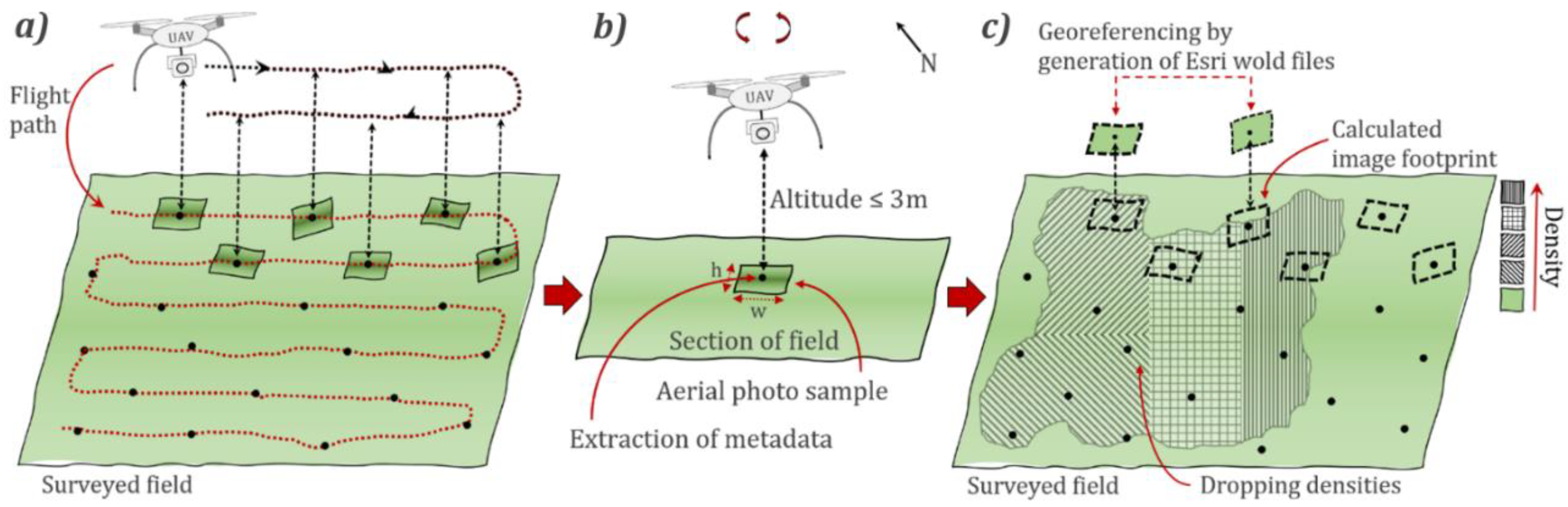
2.3. Data Collection

All UAV surveys of the ten selected fields were performed using the Pix4Dcapture application (version 4.5.0, Pix4D S.A., Prilly, Switzerland) with the integrated Free Flight mode, which was applied following the instructions described in a study from 2019 [44]. In the Free Flight mode, single photos were set to be triggered with the camera in a vertical position at intervals every time the UAV was moved three meters in any horizontal direction. These short intervals were kept to counteract the inevitable irregularity of the manual free flight and to ease the following data processing by allowing a thinning procedure with the purpose of creating regularly spaced sampling grids to enable the detection of fine-scale density alterations (Figure 2 and Supplementary Material, step ii). The fields were covered by flying in parallel lines running across the full length of the field, approximately 5–10 m distance apart. With the DJI GO application (version 3.1.52 and 4.0.6, DJI Technology Co. Ltd., Shenzhen, China), the camera shutter was set at a minimum of 1/150 of a second and the contrast was set to vivid in order to minimise image blur and enhance image details, respectively. The flying altitude above the ground, measured as the barometric altitude at take-off, was kept between 2–3 m, resulting in a photo covering an area on the ground of approximately 5 m². The maximum forward aircraft speed was 3 m/s. Airtime in the field surveyed by the UAV was approximately 30 min per hectare.

2.4. General Precision of Dropping Counts

As a precautionary measure, the precision of the dropping counts on the obtained UAV photo samples was blind-tested by comparing counting results from three different operators among the authors of this study. This was achieved by counting the areas of two test fields with different dropping densities, one with an observed high density of droppings (test field 1) and one with an observed low density of droppings (test field 2). The area covered by all three operators for test fields 1 and 2 was 389 m² distributed on 86 aerial photos and 107 m² distributed on 35 aerial photos, respectively. The photo samples collectively constituted an area of 496 m². The general counting precision was tested for significant differences using the non-parametric Kruskal Wallis test, as Bartlett’s test showed significant heterogeneity of variances (p < 0.05) [45]. Boxplots were made to illustrate the counting results for each person for the two fields, respectively.

2.5. Revised Georeferencing Workflow

By flying at altitudes below 10 m, it was not possible to automatically create orthomosaics via software such as DroneDeploy (DroneDeploy, Inc., San Francisco, CA, USA) or Pix4DMapper (Pix4D S.A., Prilly, Switzerland) of the aerial photos [46]. Consequently, it was necessary to develop a suitable practical procedure for georeferencing the UAV photos to obtain usable results, which would also be applicable for similar future studies (Figure 2). The revised georeferencing workflow was derived from descriptions in previous studies [31,47] but with several important modifications (detailed description in Supplementary Material S2). The method involved the retrieval of metadata contained in the aerial photos and generation of the Environmental Systems Research Institute (Esri) world file image extension in order to enable georeferencing in GIS software [48]. Following georeferencing of the aerial photos from the 10 fields, the single photos were then loaded into QGIS (version 3.16.14, QGIS Development Team 2022, Mountain View, CA, USA) as raster layers (Figure S3a–h). Finally, goose droppings on each of the 10 fields were manually identified and individually marked in QGIS using a shapefile point layer.

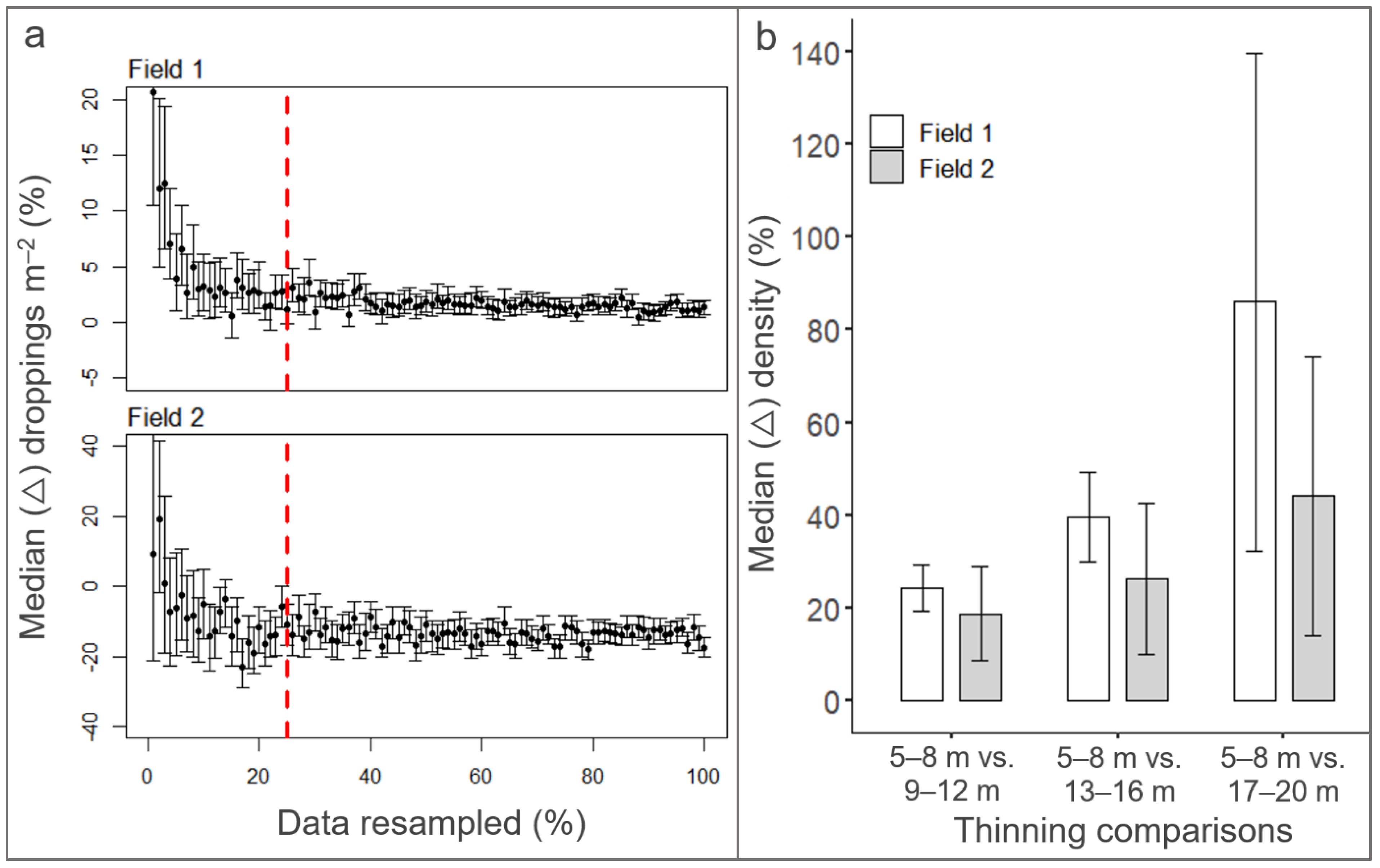
2.6. Sampling Frequency

Having georeferenced the aerial photos, an estimate of the upper limit for the spacing of the photos was performed to obtain an optimal spatial positioning in the surveying grid, applicable also for the future use of the method. The Free Flight mode, with manual horizontal piloting of the UAV, resulted in densely packed photos unequally scattered across the field. In order to create a grid of regularly spaced photo samples, thinning by the global positioning system (GPS) location of the photo centroid contained in the metadata was necessary (the protocol is described in Supplementary Material S2, step i, ii). Finding an applicable procedure to obtain a representative spacing and resulting sampling frequency of the aerial photos was an essential part of the methodology used in this study. This would minimize the working efforts of the method while simultaneously yielding a stable estimation of the dropping density (Figure 3).

The upper limit for spacing was examined by two different approaches (approaches 1 and 2) (Figure 3a,b). These approaches were tested on the two previously used test fields, which were chosen to represent the whole dataset; test field 1 had a relatively low density of droppings and a presumed low-density variation and skewness (later estimated as averaging 0.77 (0.58; 0.97 CI_95%) droppings/m² compared with a median of 0.39 (0.11; 0.50 CI_95%) droppings/m²), and test field 2 had a relatively high density of droppings with a presumed high-density variation (later estimated as averaging 6.77 (6.24; 7.22 CI_95%) droppings/m² compared to a median of 4.48 (3.99; 4.97 CI_95%) droppings/m²) (

Table 1. Properties of the 10 surveyed fields based on the 10 m sampling frequency. Listed are area (ha), number of photo samples (Ph. Samp.) from the 10 m thinning (n), median dropping density (M) per m² and mean dropping density ($\overline{\mathrm{x}}$) per m². The 95% confidence intervals ([95% CI]) are specified for both M and $\overline{\mathrm{x}}$. Further, the calculated index of dispersion (s²/$\overline{\mathrm{x}}$) and chi-square (x²) for each field are shown. Lastly, calculations of skewness (D’Agostino) and kurtosis (Anscombe-Glynn) are shown for each field and the corresponding significance levels (sign.) are specified (ns = nonsignificant, “*” < 0.05, “**” < 0.01 and “***” < 0.001).

Field (No.)	Area (ha)	Ph. Samp. (n)	Dropping Density (M)	Dropping Density ($\overline{\mathbf{x}}$)	Dispersion Index (s2/$\overline{\mathbf{x}}$)	Chi-Square (x2)	Skewness (Sign.)	Kurtosis (Sign.)
1 (test field)	2.7	106	0.31 [0.11; 0.50]	0.77 [0.58; 0.97]	1.38	144.90	1.82 (***)	6.59 (**)
2 (test field)	8.1	340	4.48 [3.99; 4.97]	6.77 [6.24; 7.22]	9.31	3156.36	2.89 (***)	14.80 (***)
3	3.3	215	1.01 [0.75; 1.28]	1.88 [1.61; 2.14]	2.93	884.48	2.01 (***)	7.43 (***)
4	7.8	282	0.60 [0.31; 0.89]	1.59 [1.30; 1.89]	2.94	629.19	1.95 (***)	6.89 (***)
5	3.9	155	0.15 [0.05; 0.26]	0.56 [0.45; 0.66]	1.46	410.32	2.14 (***)	7.47 (***)
6	5.0	181	1.19 [1.01; 1.36]	1.53 [1.36; 1.71]	0.80	122.76	0.78 (*)	2.85 (ns)
7	2.8	108	1.69 [1.42; 1.97]	2.22 [1.95; 2.50]	1.62	292.31	1.67 (***)	5.91 (*)
8	3.8	117	0.51 [0.39; 0.64]	0.67 [0.58; 0.82]	0.61	65.09	2.03 (***)	8.45 (***)
9	5.4	302	0.91 [0.43; 1.40]	1.79 [1.31; 2.27]	3.94	457.25	3.60 (***)	18.88 (***)
10	15.2	717	0.65 [0.52; 0.78]	1.30 [1.17; 1.42]	2.35	1682.77	2.27 (***)	9.80 (***)

). The discrepancy between the mean and median densities was due to the asymmetrical distribution, which was confirmed for both fields by significant values of skewness (all; p < 0.05). Initially, both test fields were thinned to approximately 5 m of spacing between each photo centroid. This was considered to represent the highest acceptable concentration of photos, as higher concentrations of photos would render the counting method practically unsuitable. This sampling corresponded to 7–9% coverage of the total area of the field, with each photo covering an average area of 4–5 m². All droppings visible on the photos were then manually counted in QGIS.

Approach 1 was performed by randomly sampling the initial photo layer of 5 m spacings with bootstrapping [49]. The goal was to determine the minimal aerial photo sampling necessary for a stable estimation of the average dropping density of the whole field (Figure 3a). The optimal spatial positioning was analysed with non-parametric bootstrapping, which was performed by randomly resampling 100 repeats of a given percentage ranging from 1–100% of the initial dataset, thereby yielding the corresponding spacing of photos ($Spacin{g}_{optimal}=\frac{Spacin{g}_{initial data}}{\% resampling of initial data}$). The mean value of the repeated samples at every percentage of the dataset was calculated together with 95% bias-corrected and accelerated (BCa) bootstrapped CI [49,50] in R [51].

In approach 2, the aim was, again, by thinning the aerial photos to determine the minimum photo sampling necessary while now simultaneously yielding a stable estimation of the differences in densities across the field (Figure 3b). In this approach, all photos with assigned numbers of droppings from the initial 5 m spacing layer were firstly binned at intervals of 5 m distances to fixed points on the two test fields. In both instances, the landscape elements were in the form of water ditches. The distances were calculated using the NNJoin plugin (version 1.3.1) in QGIS. Afterwards, the individual photos were thinned one meter at a time, starting from the initial 5 m distance and ending at 20 m, resulting in 16 thinning samples. The dropping density was then measured for each thinning sample for each distance interval to the fixed point. The differences between all 16 thinning samples (5–20 m) were determined by 95% CI of the mean, calculated as the differences in density between the thinning samples in every 5 m interval. Furthermore, to stabilise the variance and analyse 95% CI for the variance of the mean differences between comparisons, four thinning samples at a time were grouped together. The upper limit in differences for the photo thinning procedure was in the present study determined as a difference in variance not exceeding 40% relative to the mean of the grouped comparisons of 5–8 m.

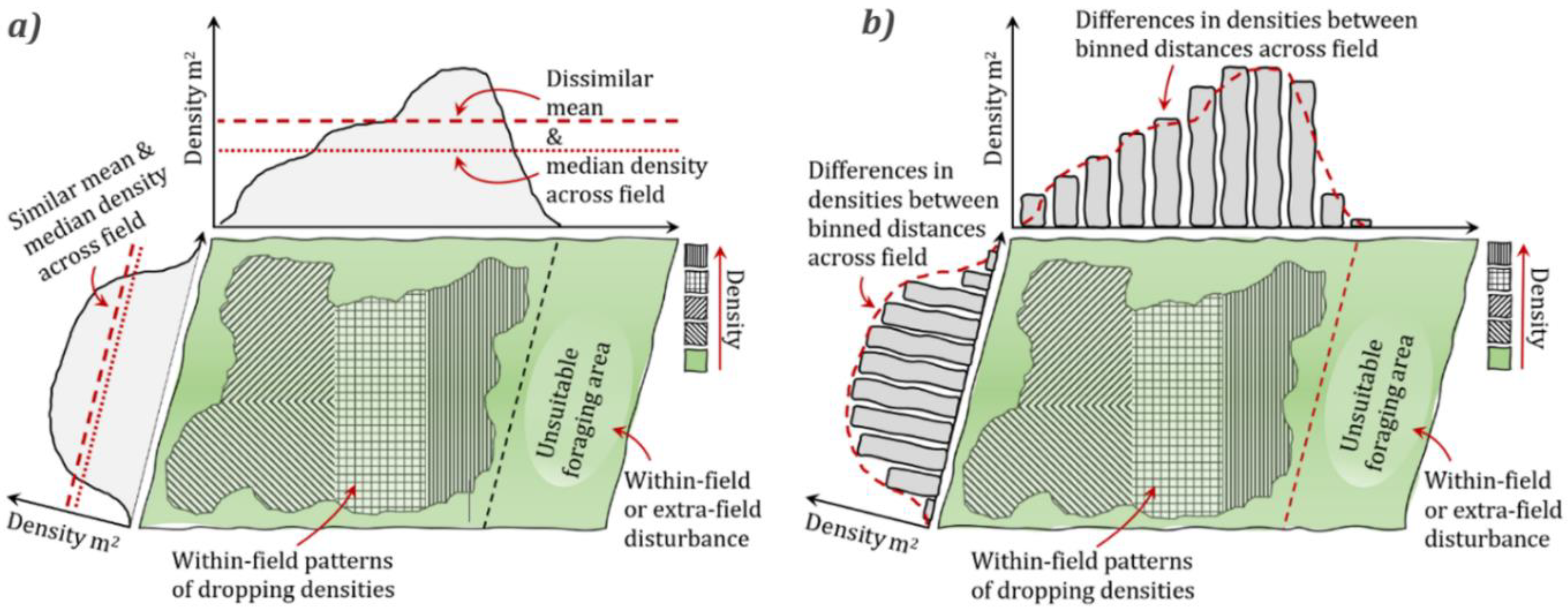
2.7. Analysis of Dropping Densities and Distribution Patterns

The distribution patterns of dropping densities in the fields were calculated by creating an index of dispersion ($inde{x}_{disp}=\frac{s^2}{\overline{\mathrm{x}}})$ to differentiate between randomly (<1), uniformly (≈1) or contagiously (clumped) (>1) dispersion [52]. Further, chi-square (χ²) values were calculated to support the evaluation of dispersion patterns, where higher values indicate a higher likelihood of clumped dispersions (${\chi }^2=inde{x}_{disp}\ast \left(n-1\right)$). Calculations of median density estimations and 95% confidence intervals (CIs) were performed for each field. Next, to perform an assessment of density distributions and field utilization, Shapiro–Wilk tests were initially performed, which showed non-normality (p = ns; all fields), allowing for calculations of skewness by the D’Agostino test [53] and kurtosis by the Anscombe–Glynn test [54].

Interpolated heatmaps over dropping densities were generated by the interpolation tool in QGIS with the TIN (triangulated irregular network) option applied. The counted dropping density for each photo position was used to interpolate with the closest other photo position. Areas covered by each photo position buffer were calculated as the area in m² of the smallest aerial photo in the field. The heatmaps were used to illustrate differences and distribution patterns of dropping densities in the surveyed fields.

Distances to all four chosen landscape elements, windbreaks, roads, water ditches and wind turbines, were measured from each of the aerial photos in the fields. Datasets for the chosen landscape elements were retrieved from the Danish Agency for Data Supply and Efficiency (SDFE), updated in 2019 [55,56]. The indexed dropping densities for all fields (consisting of 2523 aerial photos) were thinned in 25 m interval distances with respect to the three landscape elements, windbreaks, roads and water ditches, and 100 m intervals for wind turbines. Subsequently, the mean density and 95% confidence intervals were calculated for all intervals found in the combined fields.

Alterations in dropping densities were compared with the distances to the four different landscape elements, windbreaks, roads, water ditches and wind turbines. The densities for all aerial photos from all 10 fields were compared by creating a relative density index, which was achieved by dividing all dropping densities observed (obs_dens) in the field by the highest measured value for dropping density (max_dens) in the particular field. This yielded an index ranging from 0 to 1: $Density index=\frac{ob{s}_{dens}}{ ma{x}_{dens}}$. Mean densities were calculated based on 5% percentile distance intervals in the dataset and for each interval 95% bootstrapped (BCa) CI were calculated. Furthermore, to investigate the relationship between distance to landscape element and dropping density, Spearman’s rank sum correlation tests were used, and linear regressions were additionally performed.

3. Results

3.1. Maximum Flying Altitude

Accuracy in the detection of droppings of 93% and 88% compared to the manual control count from the ground could be seen when flying in altitudes ranging from 2 to 3 m above the field, respectively (Figure 4a). With further increased altitude, the accuracy dropped to 66% at 4 m and 58% at 5 m. A Tukey post-hoc test, computed based on an ANOVA, showed non-significant differences between altitudes of 2 and 3 m when compared to the ground count, whereas the altitudes of 4 and 5 m significantly differed (Figure S4 and Table S3). The flying altitudes of both 2 m and 3 m yielded 95% CI above 80%, thus qualifying both altitudes to be considered valid for the calculations of dropping densities in this study.

3.2. General Precision of Dropping Counts

No significant differences were observed when comparing the individual counting results from the three test operators for either of the two test fields chosen for validation of counting precision (both test fields with p-values > 0.05, Kruskal Wallis). This was further illustrated in boxplots showing similar values for the median, upper and lower quartiles (Figure 4b,c).

3.3. Revised Georeferencing of Aerial Photos

In this study, the development of a practical procedure for georeferencing aerial photos obtained by low altitude UAV imaging proved successful. Through the creation of Esri world files, the aerial photos could automatically be recognised and georeferenced by GIS software, which was tested in both QGIS and ArcMap (Supplementary Material S2, step i, iii and Figure S3). An important element for reliable georeferencing in this study was precise measurements of flight altitude. The occurrence of deviations in the readings of the barometric altitude during UAV flights was measured in the field up to ±0.3 m, which, at the lowest altitude of 2 m, corresponded to a possible 15% divergence in results.

3.4. Sample Frequency of Aerial Photos

High reliability of the calculated mean dropping density for the whole field (approach 1) was observed with bootstrap resampling down to 25% of the data contained in the initial sample of 5 m spacing between aerial photos, which was equivalent to a thinning of up to 20 m spacings between the photos (Figure 5a). Resampling below 25% of the dataset resulted in increasing variations in estimated mean densities and with varying CI. At 5% of the resampled data, equivalent to thinning of 100 m spacing between the aerial photos, the CI varied by up to 40%.

Thinning the aerial photos resulted, for both test fields, in increasing difference and variability in the observed distribution patterns of dropping densities across the field when compared with the initial thinning sample of 5 m spacings between the aerial photos (Figure S5, part 1–2). Subsequently, a comparison (approach 2) of the thinning samples 5–8 m against 9–12 m showed a difference of 25% for test field 1 and 35% for test field 2, both below the limit of 40% difference in dropping density and considered acceptable in this study (Figure 5b). In contrast, comparisons of 5–8 m thinning samples against 13–16 m and 17–20 m thinning samples both showed variations in dropping densities higher than 40%. Thus, a 10 m thinning of the aerial photos was henceforth applied as an acceptable spacing (Figure S6).

3.5. Dropping Density and Distribution Patterns

All estimations of the distribution patterns were based on the 10 m spacing of the aerial photos. This corresponded to an area of 2–4% out of the total field area covered by the aerial photos. The calculated index of dispersion showed that the dropping densities were contagiously distributed across the field for eight of the ten surveyed fields, with index values exceeding 1 (Table 1). For two of the fields, the dispersal could be considered randomly distributed, with values of dispersion being 0.61 and 0.80, respectively (Table 1).

Interpolation of the dropping densities by heatmaps illustrated the tendency to a contagious distribution pattern in the fields (Figure 6a,b and Figure S7). Low dropping densities could be seen at the edges for contagious distributed fields (e.g., fields 3 and 4), whereas more evenly distributed densities across the field could be seen on fields with non-contagious dropping densities (e.g., field 8).

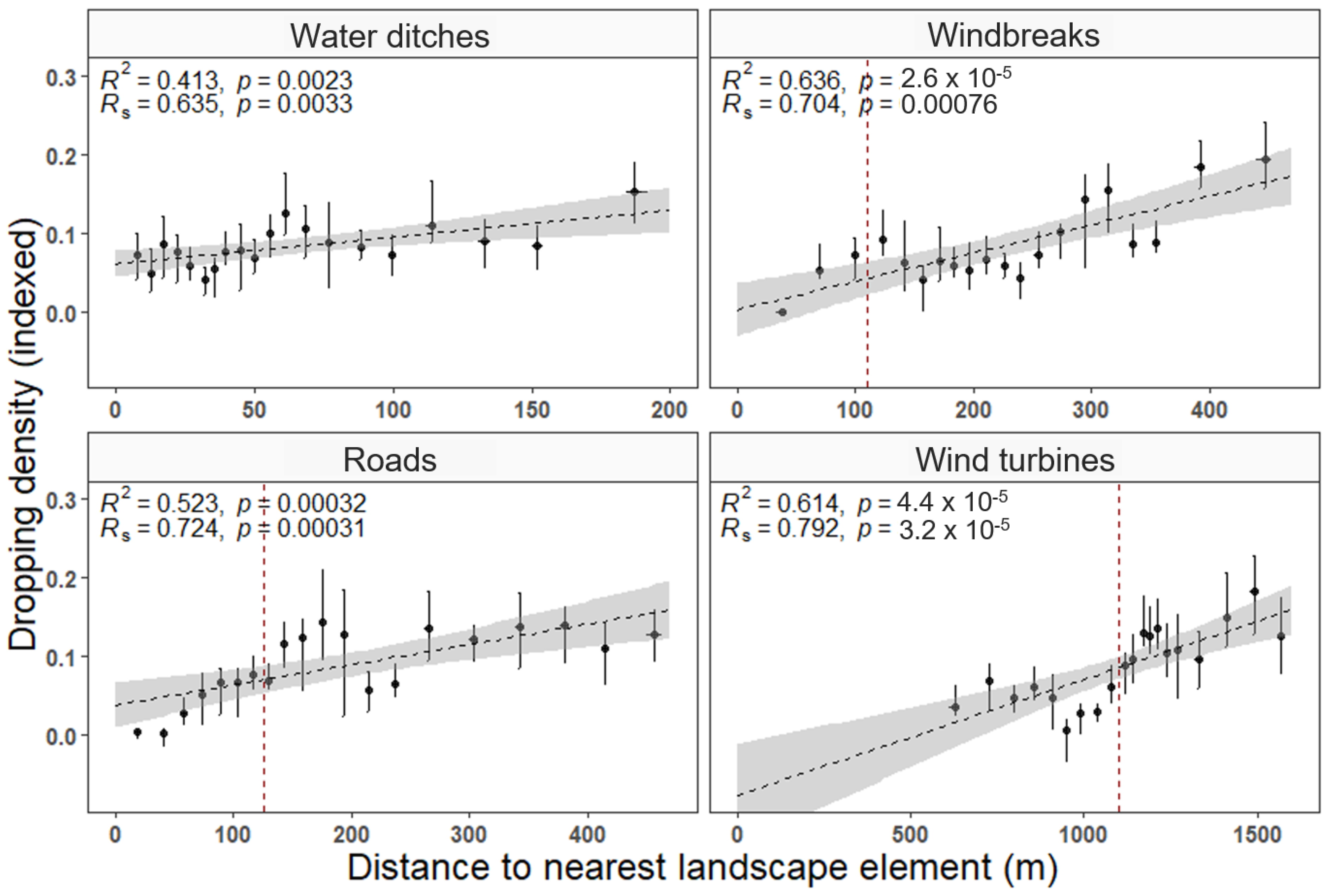
3.6. Avoidance Distances to Landscape Elements

Avoidance distances were detected for the three landscape elements, windbreaks, roads and wind turbines, with significant differences when comparing the indexed dropping densities across all surveyed fields (Figure 7). For windbreaks, a consistently lowered dropping density was observed up to 110 m with significant decreases below 75 m. For roads, the dropping density was affected up to 125 m with significant decreases below 100 m. Lastly, for wind turbines, the dropping density was significantly affected up to 1100 m (Figure 6c). For distances to water ditches, alternations in dropping density were detected with a significant tendency towards lowered density with decreased distance to the element, but no clear avoidance distances could be determined. Furthermore, for windbreaks, roads and wind turbines, local peaks appeared right after the avoidance distance ceased to influence the densities, which indicated a tendency to a skewed distribution of the dropping density.

4. Discussion

4.1. Detection of Droppings from Foraging Geese by UAV Imaging

This study showed that with UAV imaging, it was possible to detect droppings from foraging geese with acceptable accuracy, but only at low altitudes (≤3 m). It was demonstrated that flying altitude is an essential factor for reliable surveying of goose droppings with the present imaging technology available for lightweight and consumer-level UAVs with standard optical equipment [30]. To obtain acceptable results at higher altitudes, enhanced and more specialized camera equipment should be applied, exceeding that of the two quadcopters used in this study.

With flying at a low altitude came several challenges and limitations to the practical use of UAVs for the dropping count method. Certain conditions should be met, such as even surfaces in the surveyed fields, low vegetation, no protruding obstacles and keen visual observance of the UAV at all times with respect to deviations in altitude and ground levels. This imposes a substantial limit on the areas and fields applicable for surveying in general. Fortunately, the target species of geese in this study, the pink-footed goose and barnacle goose, prefer feeding in farmed areas where these conditions are often met, and such sites, in turn, were plentiful in the studied areas. The fieldwork further indicated that the most reliable results were obtained in fields with farmed grassland or pastures and that fields with winter cereals produced less accurate results, as gravel and small stones could be misidentified as droppings. Furthermore, March 2019 was particularly wet, with a precipitation rate reaching 106 mm for the month compared with the average of 45 mm [57]. This resulted in fields with newly sown crops or bare soil, which have a high washout of material, thus lowering the persistence time of goose droppings in general and on fields with bare soil in particular. On the other hand, cultivated grassland had a capacity to absorb precipitation at a higher rate beneath the mat of vegetation, leaving the goose droppings more or less unaffected [58].

The blinded counting precision test revealed a high coherence in density estimations between the three operators, all of whom had no previous experience with respect to dropping counts. This study, therefore, showed that the obtained results for dropping counts on aerial photos collected with UAVs did not depend on specific personal qualifications or previous experiences among the operators.

4.2. Successful Establishment of Revised Georeferencing Workflow

The procedure for georeferencing was time-consuming to establish but was, in the end, successful and proved afterwards to be readily applicable to the dataset. Followingly, the protocol for this revised georeferencing procedure was considered universal and thus usable for future studies requiring a similar approach and where the creation of orthomosaics is not possible. However, precautions must be taken, especially with respect to occurring deviations in the barometric altitude of the used UAVs with the potential to affect the resulting ground sample distance (GSD) and subsequent calculations of the covered m². This would not have posed a problem if the rendering of orthomosaics had been possible [31]. For use in this study, though, the measured altitude deviations of ±0.3 m during the fieldwork corresponded to ≤15% divergent results and were considered acceptable. This was acceptable as the deviations appeared equally frequent as an increase or decrease in altitude resulting in fluctuations being random with a following non-skewed sampling.

4.3. Optimal Sampling Frequencies

The results for the sampling frequency of the aerial photos firstly suggested that the average dropping density for the whole field could be highly accurately estimated with up to 20 m spacing between the photo samples and with an acceptable accuracy with spacing up to around 100 m. However, density estimations between the different parts of the field suggested that the maximum spacing between samples should not exceed 12 m. A separation of 10 m between the photo samples, corresponding to 2–4% coverage of the field, was therefore accepted as sufficiently accurate for purposes such as determining field utilisation and avoidance distances to different landscape elements. These results challenged the methodology used in other studies investigating avoidance distances by measuring dropping densities of foraging geese, where manual ground counts inside circles have been done in grids with frequencies ranging from spacings between the samples of 25 × 200 m in a study from 2000 [4] and up to 150 × 150 m in a study from 2014 [59]. Such spacings will most likely produce inconsistent results if accurate estimations of gradients in dropping density across the field are the desired outcome. However, the 5 m distance intervals to fixed points used in this study could be too fine a scale if more crude estimations are sufficient.

4.4. Assessment of Distribution Patterns and Avoidance Distances

The detection of varying distribution patterns in dropping densities on the surveyed fields in relation to the presence of external landscape elements (Figure 6) indicated that the use of UAV surveys is a useful tool to analyse and assess the behaviour of foraging geese by the indirect method of dropping counts. The highly contagious, skewed and asymmetrical dispersion patterns detected in almost all fields indicated that the behaviour of the foraging geese was likely influenced by external factors, which is in accordance with previous studies investigating dropping densities [4,60]. These factors could be stress-related effects from the surrounding landscape elements or human activities, such as possible hunting or recreational activities, which potentially can reduce the field utilisation by the geese [4,5,61]. Additionally, foraging preferences and unevenly scattered food sources on the investigated fields, perhaps resulting from some fields being partially water covered during periods of heavy precipitation earlier this spring, might also have played an important role in the fine-scale and within-field habitat selection of the geese [60].

The interpolated heatmaps further illustrated differences in density gradients with respect to both types of and distance to different landscape elements (Figure 6 and Figure 7). On the heatmaps, fields surrounded by windbreaks and roads showed a pronounced clustering away from these elements and often towards the middle of the field. In contrast to this, fields only surrounded by water ditches and no other elements nearby showed the least contagious distribution patterns (Figure 6b). This supports our assumption that water ditches can be considered the least disturbing landscape element (authors’ observations and notes). Consequently, in our study, water ditches were primarily used as a reference to check the robustness of the estimation of avoidance distances to the other landscape elements. The finding of minor decreases in density close to water ditches could be an effect of narrow buffer stripes of less nutrient-rich grass, reducing the value and attractiveness for foraging and thus should not be considered as a direct avoidance effect [3].

The significant decreases in densities for the remaining three investigated elements, wind turbines, windbreaks and roads, suggest pronounced avoidance distances to these. The results for windbreaks and roads were consistent with results found in previous studies using manual ground counts of droppings for Arctic migratory geese (pink-footed goose, greater white-fronted goose (Anser albifrons) and red-breasted goose (Branta ruficollis)) with affected dropping densities of up to 110 m for windbreaks [4,5]. For roads, the result of avoidance distances up to 125 m again corresponded well to a study from 2000 [4], which reported a 50% decrease in dropping densities of up to 150 m from larger roads. However, the results deviated from a study from 2018 [5], which found no observable avoidance distances to roads. Reasons for such inconsistencies might be due to differing usage and type of road, possibly provoking differing responses and creating varying levels of habituation.

For wind turbines, the lack of observable droppings on the UAV photos up to a radius of 600 m and further significant lowered densities up to 1100 m far exceeded the 200 m avoidance distance for clustered windfarms previously reported in 2000, despite the fact that this study [4] investigated one of the same areas as in our study, namely the Vattenfall windfarm at Klim Fjordholme. However, the wind turbines have since been replaced, and their size has increased from 67 m to more than twice the height, now reaching 150 m [62]. This increased height has most likely affected the avoidance distance to the wind turbines and very possibly in a nonlinear pattern. Another study [5] found in their study area of Bulgaria affected dropping densities at distances reaching 900 m to wind turbines of 125 m in height, suggesting that avoidance behaviour is possible at these larger distances.

General uncertainties and complications connected to dropping counts as a method to estimate avoidance distances must, however, be considered. Firstly synergistic effects of multiple landscape elements must be considered together with season and activities such as hunting [4,7]. Consequently, the variation in dropping densities indicating behavioural instabilities may also be influenced by factors, such as positive or negative spatial autocorrelations, which might occur in the study area depending on the number and character of disturbing landscape elements [63]. Also, factors such as the distribution of feeding items and standing water in the fields can possibly influence the dispersion of geese. Furthermore, it has been argued that the detection of uneven distribution patterns of the geese may be partly due to periods of roosting in the middle of the field after feeding rather than avoiding feeding at the edges because of disturbance effects [60].

Interestingly, some general and convergent tendencies were observed between the telescopic bird counts and the measured dropping densities, indicating that both the number of days with foraging geese and the number of geese present per visit determine dropping densities in the fields (authors’ notes). A combination of the two methods is therefore reasonable and will provide a broader understanding of field utilisation, where bird counts offer information on species, flock size and behaviour and where dropping counts more accurately reflect the long-term dispersion of the geese and possible avoidance distances to landscape elements.

4.5. Fields of Application

This study demonstrated that UAV imaging of dropping densities could be used as a novel and improved approach in nature management to monitor field utilisation of foraging geese. By combining UAV flights for data collection and GIS-based analysis, our method showed great potential for effective and precise detection and monitoring of shifting patterns and asymmetrical distributions, the applicability of which we evaluated for the detection of avoidance distances to landscape elements.

By using UAV imaging, improvements were demonstrated in several aspects of the fieldwork. The improvements included a quicker semi-automatic data collection with highly accurate and possible extensive photo sampling and with a reduced workload of man-hours in the field. Analyses based on the performed UAV data sampling showed that it was possible to gain unprecedented precise and realistic fine-scale estimates of density patterns for field foraging spring staging geese, pink-footed goose and barnacle goose. Furthermore, the method proved to be less invasive in terms of disturbance of the geese than manual counting in the field, as the fields can be readily surveyed with the geese absent. Additionally, during data sampling, geese foraging on adjacent fields were observed to habituate quickly to the UAV and would often forage close by and within 30 m while the data collection was performed.

However, the data processing was time-consuming as the counts on the aerial photos had to be done manually due to the existing technology of UAV and computer software available for this study. Because of the high heterogeneity of the fields, thresholding and automatic counting of droppings on the photos by existing software such as ImageJ (ImageJ, U. S. National Institutes of Health, Bethesda, MD, USA) [64] or GSA ImageAnalyser (GSA GmbH, Rostock, Germany) [65] were not applicable. To enable an easier and computer-based recognition of goose droppings for future monitoring, the camera technology of the UAV would have to be improved. This could be achieved by applying specialized filters allowing for certain wavelengths of near ultraviolet light (NUV) to be detected [66]. As animal faeces can be detected by the use of NUV light [67,68] this could, for future studies, possibly lead to far easier detection of animal faeces and, in this case, goose droppings. Additionally, it can be argued that dropping counts with UAV is best applied for estimations of the relative density in the field and not measurements of the absolute density, as the results may vary according to different conditions in the field, including the type of crops and freshness of the droppings. Finally, it was difficult to distinguish between species-specific droppings, which, however, was of minor importance in this study as the fields were predominately used by the target goose species.

References

1. Madsen, J.; Roland, O.; Fox, T. Indspil Til Forvaltning af Bramgås, Aarhus University; DCE—Danish Centre for Environment and Energy: Aarhus, Denmark, 2015; pp. 1–18. [Google Scholar]
2. Madsen, J.; Cottaar, F.; Amstrup, O.; Asfergi, T.; Bak, M.; Bakken, J.; Frikke, J.; Goma, V.; Gundersen, O.M.; Günther, K.; et al. SVALBARD PINK-FOOTED GOOSE, Aarhus University; DCE—Danish Centre for Environment and Energy: Aarhus, Denmark, 2016; pp. 5–13. [Google Scholar]
3. Chudzińska, M.E.; Van Beest, F.M.; Madsen, J.; Nabe-Nielsen, J. Using habitat selection theories to predict the spatiotemporal distribution of migratory birds during stopover—A case study of pink-footed geese Anser brachyrhynchus. Oikos 2015, 124, 851–860. [Google Scholar] [CrossRef] [Green Version]
4. Larsen, J.K.; Madsen, J. Effects of wind turbines and other physical elements on field utilization by pink-footed geese (Anser brachyrhynchus): A landscape perspective. Landsc. Ecol. 2000, 15, 755–764. [Google Scholar] [CrossRef]
5. Harrison, A.L.; Petkov, N.; Mitev, D.; Popgeorgiev, G.; Gove, B.; Hilton, G.M. Scale-dependent habitat selection by wintering geese: Implications for landscape management. Biodivers. Conserv. 2017, 27, 167–188. [Google Scholar] [CrossRef]
6. Bech-Hansen, M.; Kallehauge, R.M.; Bruhn, D.; Castenschiold, J.H.F.; Gehrlein, J.B.; Laubek, B.; Jensen, L.F.; Pertoldi, C. Effect of Landscape Elements on the Symmetry and Variance of the Spatial Distribution of Individual Birds within Foraging Flocks of Geese. Symmetry 2019, 11, 1103. [Google Scholar] [CrossRef] [Green Version]
7. Fox, A.D.; Elmberg, J.; Tombre, I.M.; Hessel, R. Agriculture and herbivorous waterfowl: A review of the scientific basis for improved management. Biol. Rev. 2017, 92, 854–877. [Google Scholar] [CrossRef]
8. Tombre, I.M.; Høgda, K.A.; Madsen, J.; Griffin, L.R.; Kuijken, E.; Shimmings, P.; Rees, E.; Verscheure, C. The onset of spring and timing of migration in two arctic nesting goose populations: The pink-footed goose Anser bachyrhynchus and the barnacle goose Branta leucopsis. J. Avian Biol. 2008, 39, 691–703. [Google Scholar] [CrossRef]
9. Bibby, C.; Burgess, N.; Hill, D.; Mustoe, S. Bird Census Techniques; Academic Press: London, UK, 2000; ISBN 0-12-095831-7. [Google Scholar]
10. Rosenstock, S.S.; Anderson, D.R.; Giesen, K.M.; Carter, M.F. Landbird Counting Techniques: Current Practices and an Alternative. Auk 2012, 119, 46–53. [Google Scholar] [CrossRef]
11. Burnham, K.P.; Anderson, D.R.; Laake, J.L. Estimation of Density from Line Transect Sampling of Biological Populations. J. R. Stat. Soc. Ser. A 1980, 144, 369. [Google Scholar] [CrossRef]
12. Frikke, J.; Laursen, K. Rastende vandfugle i Vadehavet 1980–2010. Dansk Ornitol. Foren. Tidsskr. 2013, 1, 4–26. [Google Scholar]
13. Laursen, K.; Frikke, J.; Kahlert, J. Accuracy of ‘total counts’ of waterbirds from aircraft in coastal waters. Wildlife Biol. 2008, 14, 165–175. [Google Scholar] [CrossRef] [Green Version]
14. Kempf, N.; Günther, K.; Fritz, V. Rastvögel auf Sandinseln im schleswig-holsteinischen Wattenmeer im Mai und September 2012. Die Vogelwelt 2015, 135, 167–183. [Google Scholar]
15. Sardá-Palomera; Bota, F.; Viñolo, G.; Pallarés, O.; Sazatornil, V.; Brotons, L.; Gomáriz, S.; Sadra, F.; Sardà-Palomera, F.; Bota, G.; et al. Fine-scale bird monitoring from light unmanned aircraft systems. Ibis 2012, 154, 177–183. [Google Scholar] [CrossRef]
16. Hodgson, J.C.; Baylis, S.M.; Mott, R.; Herrod, A.; Clarke, R.H. Precision wildlife monitoring using unmanned aerial vehicles. Sci. Rep. 2016, 6, 22574. [Google Scholar] [CrossRef] [Green Version]
17. Christie, K.S.; Gilbert, S.L.; Brown, C.L.; Hatfield, M.; Hanson, L. Unmanned aircraft systems in wildlife research: Current and future applications of a transformative technology. Front. Ecol. Environ. 2016, 14, 241–251. [Google Scholar] [CrossRef]
18. Wirsing, A.J.; Johnston, A.N.; Kiszka, J.J. Foreword to the Special Issue on “The rapidly expanding role of drones as a tool for wildlife research”. Wildl. Res. 2022, 49, I–V. [Google Scholar] [CrossRef]
19. Madsen, J. Relations between Change in Spring Habitat Selection and Daily Energetics of Pink-Footed Geese Anser brachyrhynchus. Ornis Scand. (Scandinavian J. Ornithol.) 1985, 16, 222–228. [Google Scholar] [CrossRef]
20. Ransom, D.; Pinchak, W.E.; Ransom, D.; Pinchak, W.E. Assessing accuracy of a laser rangefinder in estimating grassland bird density. Wildl. Soc. Bull. 2019, 31, 460–463. [Google Scholar]
21. Brennan, A.; Block, W.M.; Gutiérrez, R.J. Habitat use by mountain quail in Northern California. Condor 1987, 89, 66–74. [Google Scholar] [CrossRef]
22. Sasse, D.B. Job-related mortality of wildlife workers in the United States, 1937–2000. Wildl. Soc. Bull. 2003, 31, 1015–1020. [Google Scholar] [CrossRef]
23. McEvoy, J.F.; Hall, G.P.; McDonald, P.G. Evaluation of unmanned aerial vehicle shape, flight path and camera type for waterfowl surveys: Disturbance effects and species recognition. PeerJ 2016, 4, 1–21. [Google Scholar] [CrossRef] [Green Version]
24. Rasmussen, L.-M. Optællinger af Kolonirugende Fugle pa Fotos Optaget Med Drone Ved SNEUM Engsø, pa Langli og Holme i Limfjorden Maj 2017; Aarhus University, Institut for Bioscience: Copenhagen, Denmark, 2017. [Google Scholar]
25. Bech-Hansen, M.; Kallehauge, R.M.; Lauritzen, J.M.S.; Sørensen, M.H.; Laubek, B.; Jensen, L.F.; Pertoldi, C.; Bruhn, D. Evaluation of disturbance effect on geese caused by an approaching unmanned aerial vehicle. Bird Conserv. Int. 2019, 30, 1–7. [Google Scholar] [CrossRef]
26. Hong, S.J.; Han, Y.; Kim, S.Y.; Lee, A.Y.; Kim, G. Application of Deep-Learning Methods to Bird Detection Using Unmanned Aerial Vehicle Imagery. Sensors 2019, 19, 1651. [Google Scholar] [CrossRef] [PubMed] [Green Version]
27. Linchant, J.; Lisein, J.; Semeki, J.; Lejeune, P.; Vermeulen, C. Are unmanned aircraft systems (UASs) the future of wildlife monitoring? A review of accomplishments and challenges. Mamm. Rev. 2015, 45, 239–252. [Google Scholar] [CrossRef]
28. Valle, R.G.; Scarton, F. Drone-conducted counts as a tool for the rapid assessment of productivity of Sandwich Terns (Thalasseus sandvicensis). J. Ornithol. 2021, 162, 621–628. [Google Scholar] [CrossRef]
29. Marchowski, D. Drones, automatic counting tools, and artificial neural networks in wildlife population censusing. Ecol. Evol. 2021, 11, 16214–16227. [Google Scholar] [CrossRef] [PubMed]
30. Hughes, A.; Teuten, E.; Starnes, T.; Cowie, N.; Swinfield, T.; Humpidge, R.; Williams, J.; Bridge, D.; Casey, C.; Asque, A.; et al. Drones for GIS—Best Practice; version 2; Royal Society for the Protection of Birds Conservation: Edinburgh, UK, 2020.
31. Gotovac, D.; Kružić, S.; Gotovac, S.; Papić, V. A model for automatic geomapping of aerial images mosaic acquired by UAV. 2017 2nd Int. Multidiscip. Conf. Comput. Energy Sci. Split. 2017, 2017, 1–6. [Google Scholar]
32. Corcoran, E.; Winsen, M.; Sudholz, A.; Hamilton, G. Automated detection of wildlife using drones: Synthesis, opportunities and constraints. Methods Ecol. Evol. 2021, 12, 1103–1114. [Google Scholar] [CrossRef]
33. Vas, E.; Lescroël, A.; Duriez, O.; Boguszewski, G.; Grémillet, D. Approaching birds with drones: First experiments and ethical guidelines. Biol. Lett. 2015, 11, 201407. [Google Scholar] [CrossRef] [Green Version]
34. Mulero-Pázmány, M.; Jenni-Eiermann, S.; Strebel, N.; Sattler, T.; Negro, J.J.; Tablado, Z. Unmanned aircraft systems as a new source of disturbance for wildlife: A systematic review. PLoS ONE 2017, 12, e0178448. [Google Scholar] [CrossRef] [Green Version]
35. Owen, M. The Selection of Feeding Site by White-Fronted Geese in Winter. J. Appl. Ecol. 1971, 8, 905–917. [Google Scholar] [CrossRef]
36. Koester, V. The Ramsar Convention. In The Ramsar Convention On the Conservation of Wetlands; Ramsar Convention Bureau International Union for Conservation of Nature and Natural Resources: Gland, Switzerland, 1989; pp. 1–15. ISBN 8750374036. [Google Scholar]
37. Fox, A.D.; Ebbinge, B.S.; Mitchell, C.; Heinicke, T.; Aarvak, T.; Colhoun, K.; Clausen, P.; Dereliev, S.; Faragö, S.; Koffijberg, K.; et al. Current estimates of goose population sizes in western Europe, a gap analysis and an assessment of trends. Ornis Svecica 2010, 20, 115–127. [Google Scholar] [CrossRef] [Green Version]
38. Kjeldsen, J.P. Nordjyllands Fugle 2017. Available online: http://nordjyllandsfugle.dk/ (accessed on 10 July 2022).
39. DJI PHANTOM 4 PRO Specs. Available online: https://www.dji.com/dk/phantom-4-pro/info#specs (accessed on 1 November 2021).
40. Barr, J.R.; Green, M.C.; DeMaso, S.J.; Hardy, T.B. Drone Surveys Do Not Increase Colony-wide Flight Behaviour at Waterbird Nesting Sites, But Sensitivity Varies Among Species. Sci. Rep. 2020, 10, 3781. [Google Scholar] [CrossRef] [Green Version]
41. Castenschiold, J.H.F.; Bregnballe, T.; Bruhn, D.; Pertoldi, C. Unmanned Aircraft Systems as a Powerful Tool to Detect Fine-Scale Spatial Positioning and Interactions between Waterbirds at High-Tide Roosts. Animals 2022, 12, 947. [Google Scholar] [CrossRef] [PubMed]
42. Shapiro, S.S.; Wilk, M.B. An Analysis of Variance Test for Normality (Complete Samples). Biometrika 1965, 52, 591–611. [Google Scholar] [CrossRef]
43. Shanks, A.M.; Hutton, J.C. Bartlett’s Test. Work. Pap. 1986, 8, 1–5. [Google Scholar]
44. Davis, J. Mapping with the Phantom 3 Professional & Pix4Dcapture; Institute for Geographic Information Science, San Francisco State University: San Francisco, CA, USA, 2019. [Google Scholar]
45. Kruskal, W.H.; Wallis, W.A. Use of Ranks in One-Criterion Variance Analysis Stable. J. Am. Stat. Assoc. 1952, 47, 583–621. [Google Scholar] [CrossRef]
46. Hawkins, S. Using a drone and photogrammetry software to create orthomosaic images and 3D models of aircraft accident sites. In Proceedings of the Isasi Seminar, Reykjavik, Iceland, 17–20 October 2016; pp. 1–26. [Google Scholar]
47. Hemerly, E.M. Automatic georeferencing of images acquired by UAV’s. Int. J. Autom. Comput. 2014, 11, 347–352. [Google Scholar] [CrossRef] [Green Version]
48. Esri FAQ: What Is the Format of the World File Used for Georeferencing Images? Available online: https://support.esri.com/en/technical-article/000002860. (accessed on 1 April 2022).
49. DiCiccio, T.J.; Efron, B. Bootstrap Confidence Intervals. Stat. Sci. 1996, 11, 189–228. [Google Scholar] [CrossRef]
50. Flater, M.D. R Package ‘bootBCa.’: Function to Find Nonparametric BCa Intervals, Version 1.0. 2014. Available online: https://www.nist.gov/system/files/documents/itl/ssd/cs/bootBCa-manual.pdf (accessed on 10 July 2022).
51. R Development Core Team. R: A Language and Environment for Statistical Computing; R Foundation for Statistical Computing: Vienna, Austria, 2022. [Google Scholar]
52. Fowler, J.; Cohen, L.; Jarvis, P. Probabillity Distributions as Models of Dispersion. In Practical Statistics for Field Biology; John Wiley & Sons: Hoboken, NJ, USA, 1998; pp. 62–73. ISBN 0-471-98296-2. [Google Scholar]
53. D’Agostino, R.B.; Belanger, A.; D’Agostino, R.B., Jr. A suggestion for using powerful and informative tests of normality. Am. Stat. 1990, 44, 316–321. [Google Scholar]
54. Anscombe, F.J.; Glynn, W.J. Distribution of the kurtosis statistic b2 for normal statistics. Biometrika 1983, 70, 227–234. [Google Scholar] [CrossRef]
55. SDFE Styrelsen for Dataforsyning og Effektivisering. Available online: https://kortforsyningen.dk/content/fot-via-kortforsyningen (accessed on 22 May 2022).
56. GeoDanmark FOTspecifikation Version 5.1. Available online: http://geodanmark.nu/onewebmedia/DKPDFSpec6-Alt_B4.pdf (accessed on 10 July 2022).
57. Danish Meteorological Institute (DMI) Rekordvåd Marts 2019. Available online: https://www.dmi.dk/nyheder/2019/rekordvaad-marts-2019/ (accessed on 15 March 2022).
58. Podhrázská, J.; Uhlĺřová, J.; Hejduk, S. Evaluation of crop effects on runoff and washout of soil from the surface of agricultural land. Soil Water Res. 2009, 4, 142–148. [Google Scholar] [CrossRef] [Green Version]
59. Harrison, A.L.; Hilton, G.M. Fine-scale distribution of geese in relation to key landscape elements in coastal Dobrudzha, Bulgaria. Prelim. Rep. WWT Slimbr. 2014, 28. [Google Scholar]
60. Gill, J.A. Habitat Choice in Pink-Footed Geese: Quantifying the Constraints Determining Winter Site Use. J. Appl. Ecol. 1996, 33, 884–892. [Google Scholar] [CrossRef]
61. Laursen, K.; Kahlert, J.; Frikke, J. Factors affecting escape distances of staging waterbirds. Wildlife Biol. 2005, 11, 13–19. [Google Scholar] [CrossRef] [Green Version]
62. Achermann, C. Vindmøller ved Klim Fjordholme; Jammerbugt Kommune: Aabybro, Denmark, 2012. [Google Scholar]
63. Biswas, S.R.; Xiang, J.; Li, H. Disturbance Effects on Spatial Autocorrelation in Biodiversity: An Overview and a Call for Study. Diversity 2021, 13, 167. [Google Scholar] [CrossRef]
64. Rasband, S. ImageJ, U.S. National Institutes of Health, Bethesda, Maryland, USA. Available online: https://imagej.nih.gov/ij/ (accessed on 10 July 2022).
65. Bansemer, S.; Scheel, T. GSA Image Analyser; GSA GmbH: Rostock, Germany, 2022. [Google Scholar]
66. Kaye, T.G.; Pittman, M. Fluorescence-based detection of field targets using an autonomous unmanned aerial vehicle system. Methods Ecol. Evol. 2020, 11, 890–898. [Google Scholar] [CrossRef]
67. Kellie, A.; Dain, S.J.; Banks, P.B. Ultraviolet properties of Australian mammal urine. J. Comp. Physiol. A Neuroethol. Sens. Neural Behav. Physiol. 2004, 190, 429–435. [Google Scholar] [CrossRef] [PubMed]
68. Smith, S.L.; Hagedorn, C.; Fisher, J.A.; McDonald, J.L.; Hartel, P.G.; Mantripragada, N.S.; Dickerson, J.W.; Belcher, C.N.; Gentit, L.C.; Saluta, M.A.; et al. Exposing water samples to ultraviolet light improves fluorometry for detecting human fecal contamination. Water Res. 2007, 41, 3629–3642. [Google Scholar] [CrossRef]
69. Harvey, P. ExifTool Tag Names. Available online: http://owl.phy.queensu.ca/~phil/exiftool/TagNames/index.html (accessed on 10 July 2022).
70. Pix4Dcapture Ground Sampling Distance (GSD). Available online: https://support.pix4d.com/hc/en-us/articles/202560249-TOOLS-GSD-calculator (accessed on 10 July 2022).
71. Pix4Dcapture Camera Data Sheet. Available online: https://www.pix4d.com/product/pix4dmapper-photogrammetry-software (accessed on 10 July 2022).
Figure 1. Study area in the northern part of Jutland, Denmark. Red shaded areas indicate the investigated arable foraging sites in connection to important roost sites and Ramsar protected wetlands (green shaded areas). The fields surveyed with unmanned aerial vehicles (UAV) were distributed according to manual pre-counts of geese in the three foraging areas.
Symmetry 14 02175 g001
Figure 2. Flowchart reflecting the protocol for the georeferencing workflow for single aerial photo sampling (step-by-step details in Supplementary Material S2). (a) Unmanned aerial vehicle (UAV) surveys of the targeted fields were conducted, thereby yielding individual aerial photo samples with embedded metadata. (b) The metadata were extracted and used to calculate the image footprint on the field and orientation against north. (c) From spatial transformations derived from the metadata, an Esri world file was generated for each photo sample, and subsequent automated recognition and georeferencing in GIS software were obtained. Detection and counting of droppings on the aerial photos were performed in GIS software, which enabled fine-scale spatial annotations.
Symmetry 14 02175 g002
Figure 3. Flowcharts reflecting the objective for approaches 1 (a) and 2 (b) were both performed to determine the minimum photo sampling frequencies necessary while simultaneously sustaining a stable estimation of dropping densities in the field. In approach 1 (a), the objective was to determine the upper limit for thinning the photo samples while retaining a reliable estimation for the mean and median density of the whole field. In approach 2 (b), the objective was again to determine the upper limit for thinning the aerial photo samples while now sustaining a stable fine-scale estimation of the differences in density patterns across the field. For approach 2 this was achieved at the micro-scale level by binning the photo samples at intervals of 5 m distance to fixed points on the two test fields and comparing the results across different thinning regimes (5–20 m spacing between samples).
Symmetry 14 02175 g003
Figure 4. Detection of droppings on aerial photos (a) and accuracy of counting droppings between different operators (b,c). (a) The accuracy of detection of droppings at flying altitudes of 2, 3, 4 and 5 m compared with the corresponding ground count. All tests were performed in circles of 40 cm in radius (0.53 m2). The number of replications was 15 (n = 15). Vertical lines represent 95% confidence intervals (CIs). The horizontal line represents the lower limit of 80% accuracy from the ground count, wherein all of the 95% CI of the mean should be located to be considered valid in this study. b,c) Boxplots for counting precision among three different operators (Op. 1, Op. 2 and Op. 3) on the two test fields 1 (b) and 2 (c). The density was measured as droppings per m2 of the total counted area of test fields 1 and 2, of 389 m2 and 107 m2, respectively.
Symmetry 14 02175 g004
Figure 5. Results for approaches 1 (a) and 2 (b) to determine an optimal sampling frequency. For approach 1 (determination of median density of the whole field), the results, as median differences (∆), are shown for the bootstrapped resampling of the median density per m2 for test fields 1 and 2. Vertical lines represent 95% bias-corrected and accelerated (BCa) confidence intervals (CIs), and the red dashed vertical line indicates 25% resampling of the data. The resampling percentage resulted in high reliability for the calculated median dropping density. For approach 2 (determination of density patterns across the field), the relative difference in dropping density per m2 for test fields 1 and 2 were tested at intervals of 5 m from 0–80 m to the nearest fix point (water ditch). Each of the 16 thinning samples (5–20 m spacings of aerial photos) was then compared with each other, and the median difference was calculated. In order to allow for a more stable comparison, the thinning samples were grouped four at a time (5–8, 9–12, 13–16 and 17–20 m). The grouped interval of 5–8 m was used as the base with which the other grouped intervals were compared. Vertical lines represent 95% CI. The total number of registered droppings was 1316 for test field 1 and 41,191 for test field 2 at 5 m spacing of photos. The area of the tested fields was 2.7 and 8.1 hectares for test fields 1 and 2, respectively.
Symmetry 14 02175 g005
Figure 6. Map sections extracted from QGIS show examples of interpolated heatmaps for the dropping densities of (a) two contagiously distributed fields with possible disturbance from surrounding landscape elements, windbreaks and roads, and (b) one field with a more randomly distributed density and only water ditches surrounding the field in a radius of +200 m. (c) The possible effects of landscape elements on the complete study area at Klim Fjordholme, in proximity to several landscape elements, including wind turbines, roads and windbreaks. Closest wind turbines to the investigated fields are circled with radiating shading. The heatmap values span from zero droppings (white colour) to the maximum number of droppings per aerial photo of the particular field (dark red colour).
Symmetry 14 02175 g006
Figure 7. Alterations in dropping densities compared with distances to the four different landscape elements, windbreaks, roads, water ditches and wind turbines. The densities are shown for all aerial photos from all 10 fields, which were compared by creating a relative density index, where one is the aerial photo with the highest density per m2 in a particular field, and zero is the aerial photo with the lowest density. Median densities are calculated based on 5% percentile distance intervals in the dataset. Vertical and horizontal lines represent 95% bias-corrected and accelerated (BCa) bootstrapped confidence intervals (CI). For each landscape element, linear regression is depicted (dotted line), adhering to standard error (SE) for R2 and p-values for the regression slope. Spearman’s rank sum correlation values are depicted (Rs). Consistently decreased densities at lowered distances are denoted for three of the four landscape elements (dashed red vertical lines). Tests were performed and denoted for each landscape element (Rs). The total number of aerial photos for all fields was 2523, and the number of individual droppings was 35,385 in total.
Symmetry 14 02175 g007