
Energy of Vague Fuzzy Graph Structure and Its Application in Decision Making

1
Shenzhen Tourism College, Jinan University, Shenzhen 518053, China
2
Guangdong Polytechnic of Science and Technology, Guangzhou 510640, China
3
Department of Mathematics, University of Mazandaran, Babolsar 4741613534, Iran
4
School of Mathematics, Damghan University, Damghan 3671641167, Iran
*
Author to whom correspondence should be addressed.
Symmetry 2022, 14(10), 2081; https://doi.org/10.3390/sym14102081
Submission received: 6 September 2022
/
Revised: 27 September 2022
/
Accepted: 2 October 2022
/
Published: 6 October 2022
Abstract
:Vague graphs (VGs), belonging to the fuzzy graphs (FGs) family, have good capabilities when faced with problems that cannot be expressed by FGs. The notion of a VG is a new mathematical attitude to model the ambiguity and uncertainty in decision-making issues. A vague fuzzy graph structure (VFGS) is the generalization of the VG. It is a powerful and useful tool to find the influential person in various relations. VFGSs can deal with the uncertainty associated with the inconsistent and indeterminate information of any real-world problems where fuzzy graphs may fail to reveal satisfactory results. Moreover, VGSs are very useful tools for the study of different domains of computer science such as networking, social systems, and other issues such as bioscience and medical science. The subject of energy in graph theory is one of the most attractive topics that is very important in biological and chemical sciences. Hence, in this work, we extend the notion of energy of a VG to the energy of a VFGS and also use the concept of energy in modeling problems related to VFGS. Actually, our purpose is to develop a notion of VFGS and investigate energy and Laplacian energy (LE) on this graph. We define the adjacency matrix (AM) concept, energy, and LE of a VFGS. Finally, we present three applications of the energy in decision-making problems.
1. Introduction
In this modern epoch of technology, modeling uncertainties in engineering, computer sciences, social sciences, medical sciences, and economics is growing extensively. Classical mathematical methods are not always useful for dealing with such problems. FG models are advantageous mathematical tools for solving problems in various aspects. Fuzzy graphical models are obviously better than graphical models because of the natural existence of vagueness and ambiguity. The subject of a fuzzy set (FS) was introduced by Zadeh [1] in 1995. After the introduction of fuzzy sets, FS theory has included a large research field. Since then, the theory of FSs has become a vigorous area of research in different disciplines including life sciences, management, statistic, graph theory, and automata theory. The subject of FGs was proposed by Rosenfeld [2]. Kaufmann [3] presented the definitions of FGs from the Zadeh fuzzy relations in 1973. Akram et al. [4,5,6] introduced several concepts in FGs. Some of these product operations on FGs were presented by Mordeson and Peng [7]. Gau and Buehrer [8] proposed the concept of vague set (VS) in 1993 by replacing the value of an element in a set with a subinterval of . One type of FG is VG. VGs have a variety of applications in other sciences, including biology, psychology, and medicine. Moreover, a VG can concentrate on determining the uncertainties coupled with the inconsistent and indeterminate information of any real-world problems where FGs may not lead to adequate results. Ramakrishna [9] introduced the concept of VGs and studied some of their properties. After that, Akram et al. [10] introduced vague hypergraphs. Borzoei and Rashmanlou [11,12,13] investigated different subjects of VGs. Rao et al. [14,15,16] studied certain properties of domination in vague incidence graphs. Shi et al. [17,18] investigated the domination of product VGs with an application in transportation. Qiang et al. [19] defined novel concepts of domination in vague graphs. New concepts of coloring in vague graphs are presented by Krishna [20]. A graph structure (GS) is a generalization of simple graphs. GSs are very useful in the study of different domains of computer science and computational intelligence. Borzoei and Rashmanlou [21] presented the concept of the maximal product of graphs under a vague environment. Akram et al. [22,23,24] investigated certain types of vague cycles, vague trees, and Cayley vague graphs. First, Sampathkumar [25] introduced the notion of a GS. Fuzzy graph structures (FGSs) are more useful than GSs because they involve the uncertainty and ambiguity of many real-world phenoms. Dinesh [26] introduced the notion of FGSs and investigated some related concepts. Ramakrishna and Dinesh [27] expressed generalized FGSs. Kosari et al. [28,29] presented the notion of VG structure with an application in the medical diagnosis, and they studied a novel description of VG with an application in transportation systems. VGSs are the generalization of FGSs and are powerful tools in the explanation of some structures. Moreover, VFGSs are more applicable than GSs because they confront the uncertainty and ambiguity of many real-world problems. Specific properties of a VFGS are investigated, including the order of a VFGS, the degree of a vertex, and various types of energy in VFGS. Talebi et al. [30] studied the interval-valued fuzzy graph with an application in energy industry management.
Tchier et al. [31] expressed a new group decision-making technique under picture fuzzy soft expert information. Alolaiyan et al. [32] presented a novel MADM framework under q-Rung orthopair fuzzy bipolar soft sets. Akram et al. [33,34] introduced a new notion of pythagorean fuzzy matroids with application and also expressed new results of group decision-making with fermatean fuzzy soft expert knowledge.
Gutman [35], in 1978, presented the notion of graph energy. Certain bounds on energy are discussed in [36,37,38]. The energy of the graph is extended to the energy of FG by Anjali and Sunil Mathew [39] in 2013. Moreover, the energy of an FG is extended to the energy of an intuitionistic fuzzy graph by Praba and Deepa [40] in 2014. Naz et al. [41] extended the energy of an FG to the energy of a bipolar fuzzy graph in 2018. Shi et al. [42] extended the energy on picture fuzzy graphs in 2022. In 2006, Gutman and Zhou [43] defined the Laplacian energy (LE) of a graph as the sum of the absolute deviations (i.e., the distance from the mean) of the eigenvalues of its Laplacian Matrix (LM). Although VGs are better at expressing uncertain variables than FGs, they do not perform well in many real-world situations, such as IT management. Therefore, when the data come from several factors, it is necessary to use VFGSs. Belonging to the FG family, VFGSs have good capabilities when facing problems that cannot be expressed by VGs and GSs. VFGSs have several applications in real-life systems and applications where the level of information inherited in the system varies with time and has different accuracy levels. In this paper, we developed the energy on a VFGS and investigated its properties. We want to solve real problems through the energy applications of this graph. Considering the decision making, a method was suggested to rank the available options using the VFGS and its LE.
2. Preliminaries
Definition 1
([30]). A fuzzy graph on a graph is a pair where ξ is a fuzzy set on W, and χ is a fuzzy set on E, such that,
for all
Definition 2
([8]). A vague set (VS) Q is a pair on set W, where and are real valued functions which can be defined on so that,
Definition 3
Definition 4
The order of G is defined as
Definition 5
([25]). A graph structure (GS) contains a non-empty set W with relations on set W that are separated such that each relation is symmetric and irreflexive. The GS can be described as similar as a graph, where each edge is labeled as .
Definition 6
([27]). Suppose ζ be the FS on W and be FSs on , respectively. If for all , then is called FGS of GS .
is named a VFGS of a GS if is a VS on W, and for every , is a VS on such that:
Note that , for all and , , where W and are named the underlying vertex set and underlying i-edge set of G, respectively.
Example 1.
Consider a graph structure , where , , , and . Suppose Q, , , and is a vague fuzzy subset of W, , , and , respectively, such that
Then, is a VFGS on as shown in Figure 1.
Definition 7.
Two vertices that are connected by an edge are named adjacent. The AM for a graph is a matrix with n rows and m columns, , and its entries are defined by
Definition 8.
The spectrum of a matrix is defined as a set of its eigenvalues, and we denote it with . The eigenvalues , of the AM of G are the eigenvalues of G. The spectrum of the AM of G is the ; the eigenvalues of the graph satisfy the following relations:
Definition 9.
The energy of a graph G is denoted by and is defined as the sum of the absolute values of the eigenvalues of , that is,
where is an eigenvalues of
Theorem 1.
Suppose that G is a graph with l vertices and k edges and is the AM of G then
All the essential notations are shown in Table 1.
3. Energy of a Vague Fuzzy Graph Structure
In this section, we express a new notion of the extension of the energy of an FGS called VFGS. We define the notion of energy of a VFGS which can be used in real science.
Definition 10.
The AM of a VFGS, is defined as , where , is a square matrix as in which , where and represent the strength of relationship between and , respectively.
Definition 11.
The energy of a VFGS is defined as the following:
with
where and are eigenvalues of and , respectively.
Example 2.
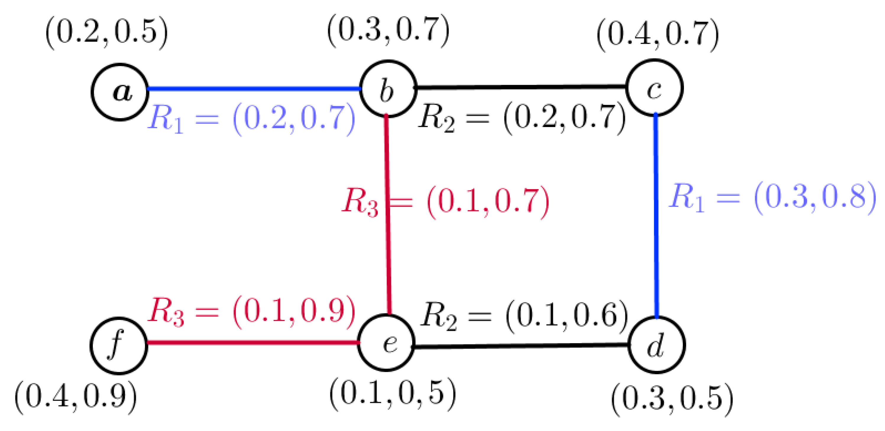
Consider a GS , where , , and . Suppose Q, , , and is a vague fuzzy subset of W, , , and , respectively, then, is a VFGS on as shown in Figure 2, such that
The AMs and energy of each degree of G are obtained as follows:
Therefore, the energy of a VFGS is equal to
Theorem 2.
Suppose that is a VFGS and is its AM. If and are the eigenvalues of and , respectively, then,
Proof.
where
- (I)
- Since is a symmetric matrix with zero trace, its eigenvalues are real with a sum equal to zero.
- (II)
- By effect properties of the matrix, we have
Hence,
Moreover, we have,
where
Hence,
□
Theorem 3.
Let be a VFGS and be the AM of G. Then,
- (I)
- (II)
Proof.
(I) Applying Cauchy–Schwarz inequality to the vectors and
with n entries, we obtain:
By comparing the coefficients of in the characteristic polynomial
we have
By replacing (3) in (2), we obtain
Replacing (4) in (1), we obtain:
Therefore,
Since
also, since
so,
Thus,
Similarly, we can prove cases (II). □
Theorem 4.
Suppose is a VFGS and is a AM of If then
Proof.
(I) If is a symmetric matrix with zero trace, then , where is the maximum eigenvalue of . If is the adjacency matrix of a VFG G, then, , where . Moreover, since
Applying Cauchy–Schwarz unequality to the vectors and
with entries, we obtain
Replacing (5) in (6), we must have
Now, the function decreases on the interval
Moreover,
So,
Therefore, (7) implies
Similarly, we can prove cases (II). □
Theorem 5.
Suppose is a VFGS. Then,
Proof.
Let be a VSFG. If , then by usual calculus, it is clear to show that is maximized when Replacing this value of g in place of , we must have .
Similarly, it is easy to show that . Hence, . □
Definition 12.
Suppose is a VFGS on n vertices. The degree matrix of G is an diagonal matrix, which is defined as:
Definition 13.
The of a VFGS is defined as , where and are the degrees matrix and AM of a VFGS, respectively.
Definition 14.
The of a VFGS is defined as the following:
where
and are the eigenvalues of and .
Example 3.
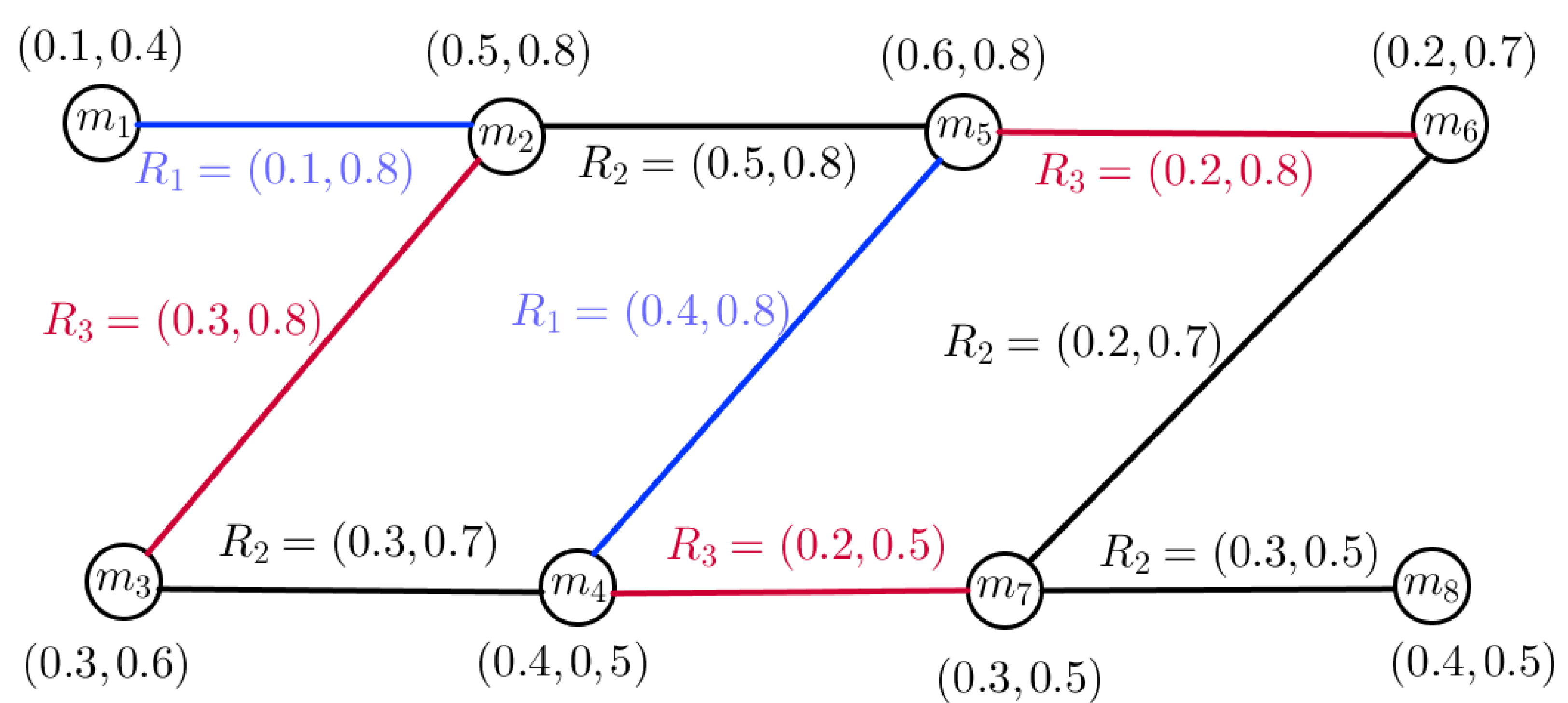
Consider a GS , where , , and . Suppose Q, , and are a vague fuzzy subset of W, , and , respectively, then, is a VFGS on as shown in Figure 3, such that
The AMs and energy of each degree of G are obtained as follows:
Therefore, the energy of a VFGS is equal to
The degree matrix and are as follows:
According to the relationship , we have
After computing, we have and
According to the relationship , we have
After computing, we have and
Therefore, the of a VFGS is equal to
Theorem 6.
Suppose that is a VSFG and is the of G. If and are the eigenvalues of and , then
Proof.
where
- (I)
- Since is a symmetric matrix with non-negative Laplacian eigenvalues, therefore,Then, , similarly, .
- (II)
- By tracing the properties of the matrix, we have
Hence,
Similarly, the other relations are fixed. □
Theorem 7.
Suppose is a VFGS on n vertices and is the of G, then
- (I)
- (II)
Proof.
(I) Applying Cauchy–Schwarz inequality to the vectors and
with n entries, we obtain
since
Therefore, we have
Similarly, we can prove cases (II). □
Theorem 8.
Suppose is a VFGS and is a of G. Then
- (I)
- (II)
Proof.
Using the Caushy–Schwarz inequality, we obtain
Since
Therefore,
Similarly, we can prove cases (II). □
4. Applications of the Energy VFGS in Decision Making
4.1. Designing an Organizational Communication System
In the real world, communication is very important in every sector, and one of the things we want to talk about is organizational communication. Organizational communication has attracted the attention of many behavioral and organizational science thinkers to the extent that many organizational difficulties have been analyzed and suitable solutions have been found for them. Some thinkers of organizational communication, such as management consultants who have been studying organizational inadequacies in recent years, believe that many of the issues and problems governing organizations are a result of incorrect communication context and lack of attention to the subtleties of organizational communication. If the managers were aware of these issues, they would probably perform their work more effectively and efficiently. With the continuation of interactions between employees, communication networks are formed naturally. Because duties, relations, and memberships are changing, the connections are not fixed and permanent. According to these concepts, we present an example of multiple organizational relationships and examine the importance and impact of multiple relationships in increasing the efficiency and success of an organization.
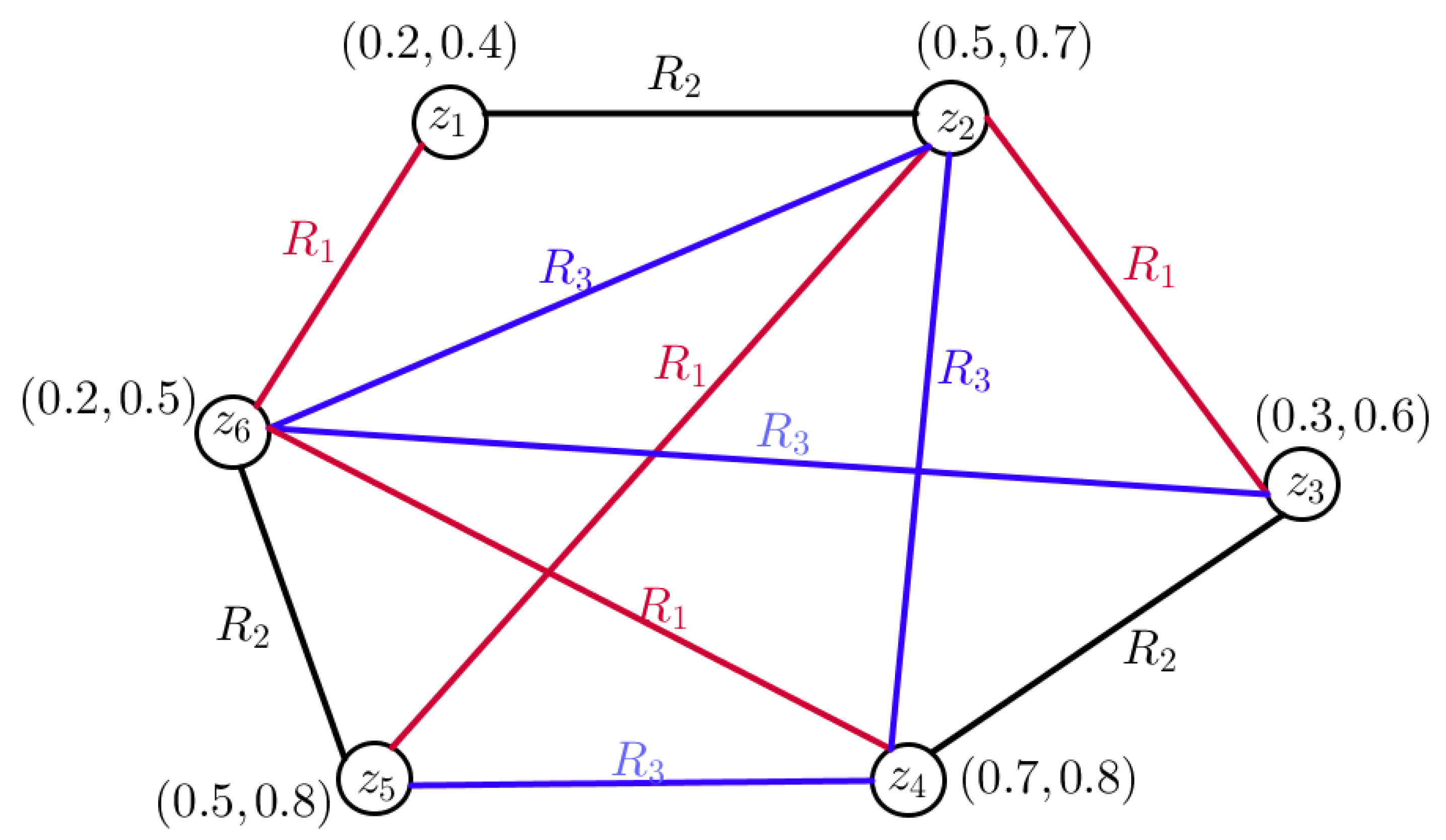
In this example, we consider education organization as a graph whose vertices include organization management (), financial vice president (), education unit (), educational vice president (), technology unit (), and research unit (). In this educational organization, we want to examine the three desired relationships between the introduced units’ efficient manpower (), improving the scientific and educational level (), and the relationship between salaries and benefits in raising the quality and efficiency of the organization ().
Here, we consider a set of units Q and a set of relations . Consider organization management, financial vice president, education unit, educational vice president, technology unit, research unit } as a set of units in an education organization and efficient manpower, improving the scientific and educational level, } as sets of relations between units of an education organization.
Now, in Figure 4, we assume is the VFGS, where is the set of vertices and , , and are sets of relations between vertices in this graph.
In Figure 4, it is clear that there are three different relationships between the units; we first obtain the energy of each relationship. The AMs and energy of each degree of G are obtained as follows:
Therefore, the energy of a VFGS is equal to
The degree matrix and are as follows:
According to the relationship , we have
After computing, we have and
According to the relationship , we have
After computing, we have and
According to the relationship , we have
After computing, we have and
Therefore, the of a VFGS is equal to .
In this application, we can clearly see that if the amount of energy in the relationships between the units is greater, the units have a greater impact on each other. Here, it is clear that the energy in is more than others. Therefore, the educational vice president unit and technology unit, education unit and research unit, education unit and educational vice president unit, and education unit and research unit have a greater effect on each other.
4.2. Role of Virtual Social Networks on Cultural Communication
Virtual space has entered many areas of life in different human societies in such a way that it is used for various purposes, including business, games and entertainment, and similar work activities, and the beneficiaries of individuals and institutions use these virtual spaces to facilitate work or provide special services. Currently, social networks are the inhabitants of the turbulent ocean of the Internet. Networks play an essential role in the world’s media equations with virtual socialism. The virtual space is formed depending on social constructions, and technological growth, media convergence, and related issues are different outputs in different social conditions. Virtual social networks, such as Twitter, Instagram, Facebook, WhatsApp, Telegram, etc., which provide the opportunity to meet people from different cultures with different languages and ethnicities, are very important in intercultural communication, and since in Iran the application of virtual social networks is widespread, these virtual social networks are considered an important source for the intercultural communication of Iranians. Due to the fact that today’s era is the era of communication and virtual space, it is not possible to communicate in this space without accepting cultures and accepting cultures without taking into account customs and beliefs and, ultimately, creating a common culture. Therefore, the main issue of this application is the role of virtual social networks in cultural communication in Iran.
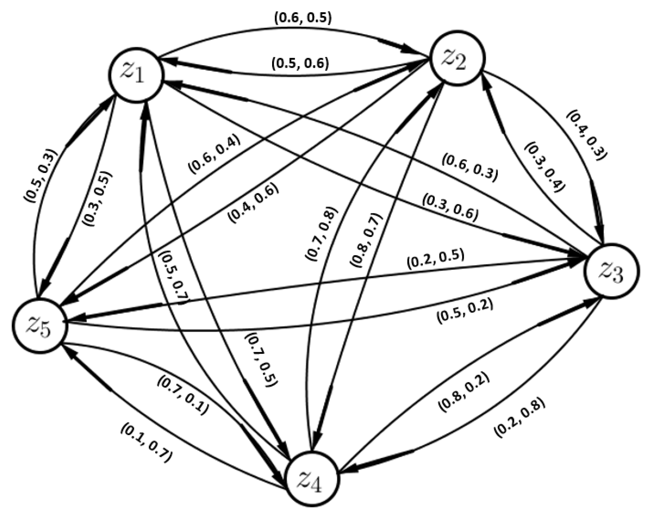
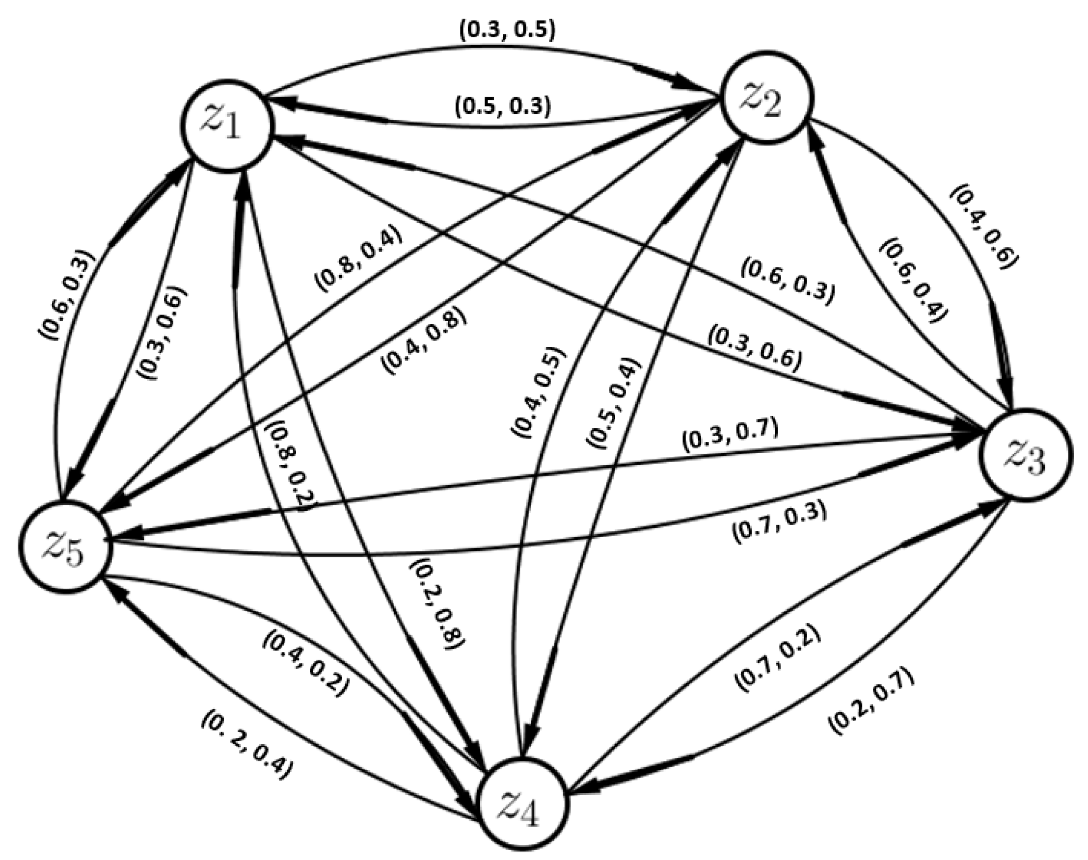
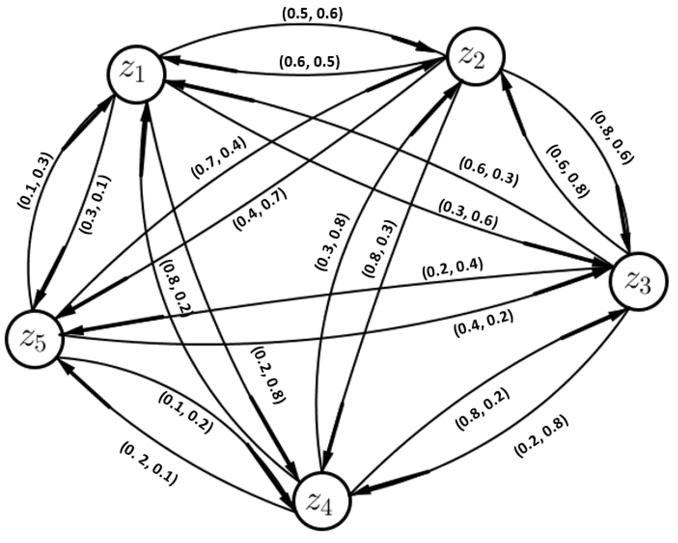
We used five platforms : Twitter (), Instagram (), Facebook (), WhatsApp (), and Telegram () to investigate the role of virtual space in cultural communication. Meanwhile, we invited four experts in the field of cultural issues to examine each of these platforms’ vague fuzzy preference relations (VFPRs) as follows:
The VFDGs corresponding to VFPRs given in matrices are shown in Figure 5, Figure 6, Figure 7 and Figure 8, respectively
The energy of each VFDG is calculated as:
, and
Then, the weight of each expert can be calculated as:
Here,
Therefore, the weight vector of four experts is:
Compute the averaged vague fuzzy element (VFE) of the platforms (Twitter (), Instagram(), Facebook (), WhatsApp (), and Telegram ()) over all the other testing venues for the experts by the vague fuzzy averaging (VFA) operator:
The aggregation results are listed in Table 2.
Compute a collective VFE of the platforms ( Twitter (), Instagram (), Facebook (), WhatsApp(), and Telegram ()) over all the other platforms using the vague fuzzy weighted averaging (VFWA) operator [32]:
Therefore, Twitter (, Instagram (, Facebook (, Whatsapp (, and Telegram (
Compute the score functions [33] of and rank all the platforms ( Twitter (), Instagram (), Facebook (), WhatsApp (), and Telegram ()) according to the values of (Twitter (), Instagram (), Facebook (), WhatsApp (), and Telegram()).
Then, Thus, the best platform is WhatsApp.
4.3. Role of Advertising Tools in Raising the Quality Level of Advertising Companies
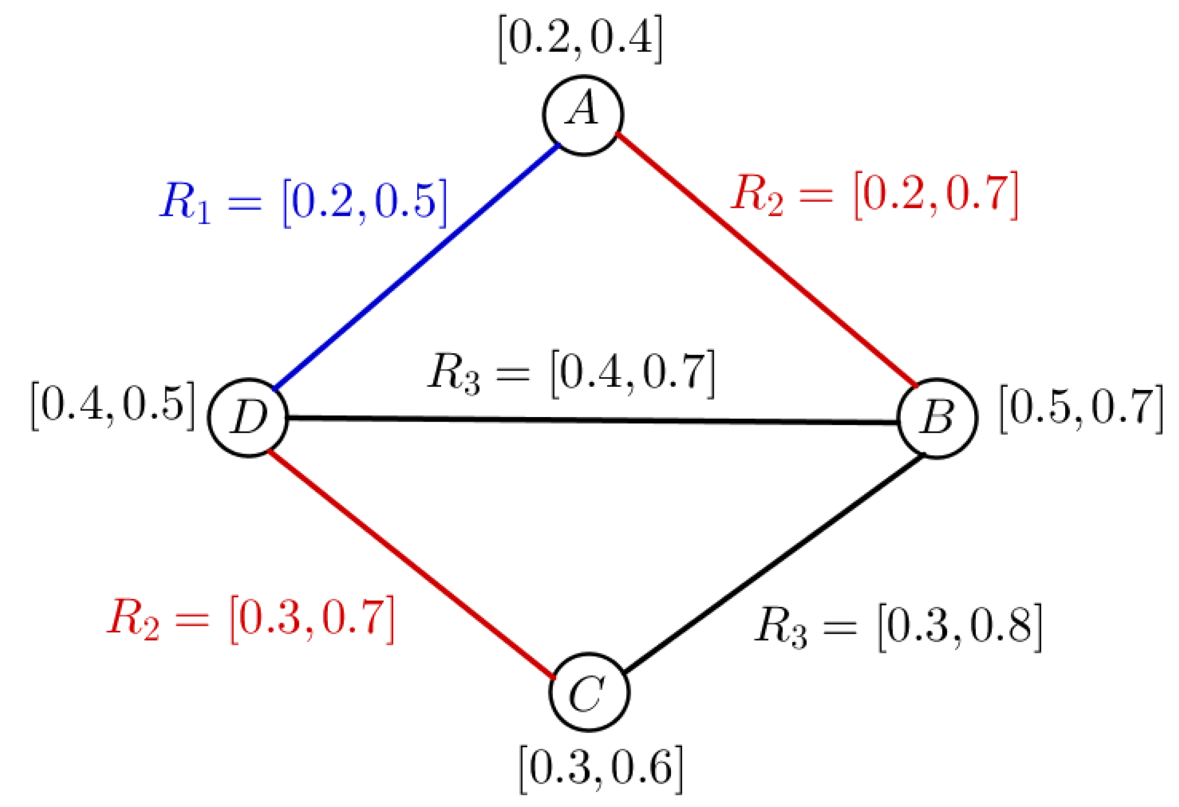
An advertising company is a company that creates, plans, and manages all aspects of advertising for its customers. Advertising companies can specialize in a specific field and branch of advertising, such as interactive advertising, or comprehensively provide services and use all advertising tools such as websites, social media, online advertising, etc. Brochures, catalogs, instant messaging with direct mail, print media, television ads, sales invitations, etc., are among the advertising tools that the advertising company uses to operate in this field. In this part, four advertising companies signed contracts among themselves to raise the quality level of their work. In these contracts, the companies defined relationships between themselves. In their meeting, these four companies expressed the factors that can affect their work promotion, among which are the right price regarding the quality, the professional production group, company services, and customer orientation. We assume that there are four advertising companies with the names , and D. We define the relationships between them as follows,
Consider as a set of advertising companies and creating television teasers (), designing and printing billboards (), advertising photography () } as sets of relations between advertising companies.
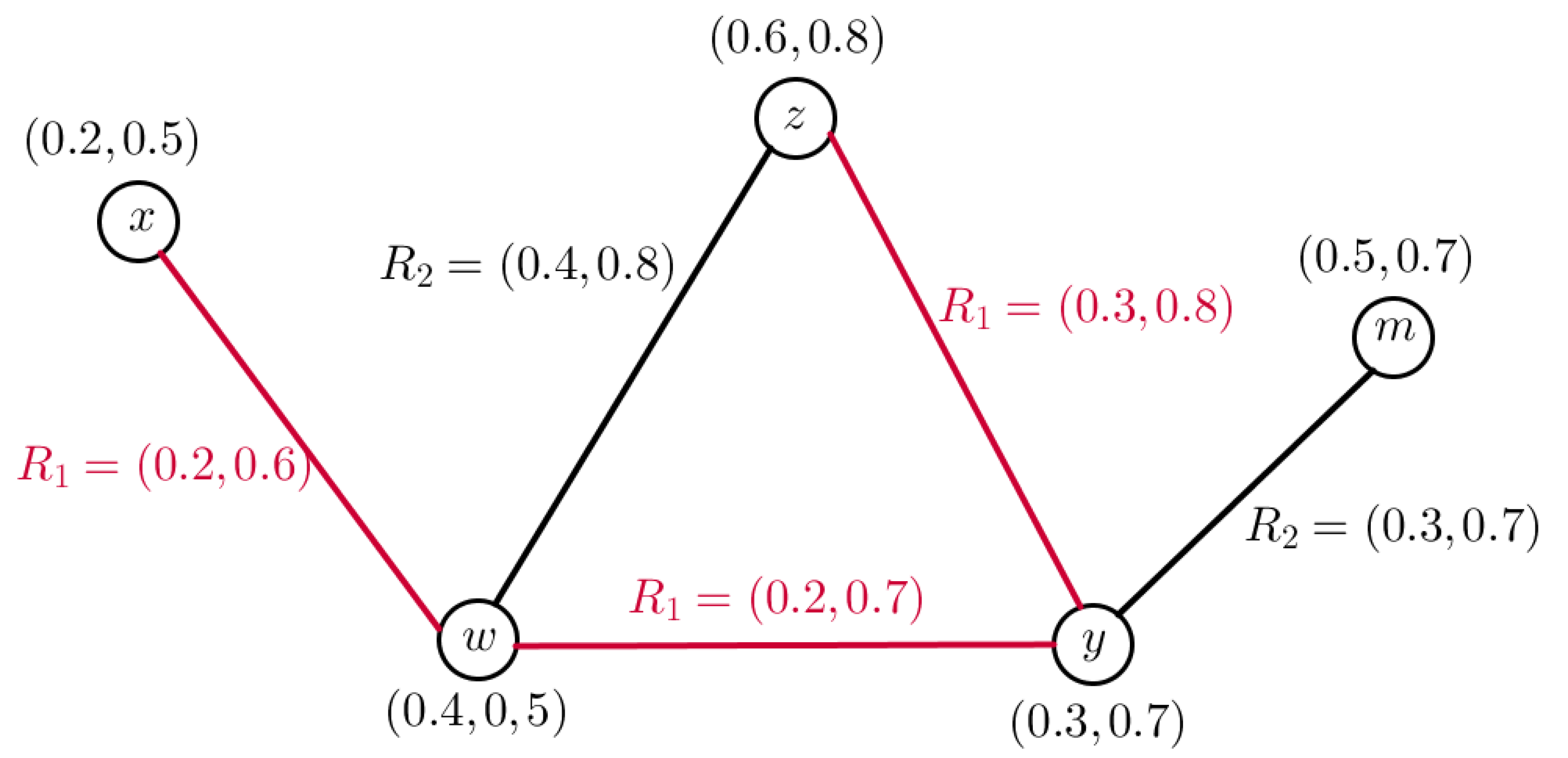
Now, in Figure 9, we assume is the VFGS, where is the set of vertices and , and are sets of relations between vertices in this graph.
In Figure 9, it is clear that there are three different relationships between the advertising companies; we first obtain the energy of each relationship. The AMs and energy of each degree of G are obtained as follows:
Therefore, the energy of a VFGS is equal to
The degree matrix and are as follows:
According to the relationship , we have
After computing, we have and
According to the relationship , we have
After computing, we have and
According to the relationship , we have
After computing, we have and
Therefore, the of a VFGS is equal to
.
In this application, we can clearly see that if the amount of energy in the relationships between the advertising companies is greater, they have a greater impact on each other. Here, it is clear that the energy in is more than others. Therefore, in order to raise the quality level of their work, two companies A and B, and also two companies C and D, can cooperate in the field of designing and printing advertising billboards.
5. Conclusions
Graph theory has many applications in solving different problems of several domains, including networking, planning, and scheduling. VGSs are very valuable tools for the study of various domains of computational intelligence and computer science. Optimization, neural networks, and operations research can be mentioned among the applications of VGSs in different sciences. Since many parameters in real-world networks are specifically related to the concept of energy, this concept has become one of the most extremely used concepts in graph theory. However, the energy in FG is so important because of the confrontation with uncertain and ambiguous topics. This concept becomes more interesting when we know that we are dealing with an FG called VFGS. This led us to examine the energy in VFGSs. So, in this work, we presented the notion of the energy of a VFGS and investigated some of its properties. We obtained the energy of the VFGS by using the eigenvalues of the AM and calculating its spectrum. Moreover, we expanded the concept of the LE on a VFGS. Finally, three applications of the VFGS in decision making are presented. In our future work, we will investigate the concepts of domination set, vertex covering, and independent set in VGSs and give applications of different types of domination in VGSs and other sciences.
Author Contributions
S.L., C.W. and A.A.T.; methodology, C.W., M.M. and S.L.; validation, C.W. and A.A.T.; formal analysis, S.L. and M.M.; investigation, M.M., A.A.T. and C.W.; data curation, A.A.T., C.W. and S.L.; writing—original draft preparation, S.L. and A.A.T.; writing—review and editing, C.W., A.A.T. and M.M.; visualization, M.M., S.L. and C.W.; supervision, C.W. and project administration, S.L. and A.A.T.; funding acquisition, S.L. All authors have read and agreed to the published version of the manuscript.
Funding
(1) the Special Projects in Key Fields of Colleges and Universities of Guangdong Province (New Generation Information Technology) under Grant No.2021ZDZX1113. (2) Continuing Education Quality Improvement Project of Department of Education of Guangdong Province under Grant No.JXJYGC2021FY0415. 5G+ Smart Community Education Demonstration Base.
Conflicts of Interest
The authors declare no conflict of interest.
References
- Zadeh, L.A. Fuzzy set. Inf. Control. 1965, 8, 338–353. [Google Scholar] [CrossRef] [Green Version]
- Rosenfeld, A. Fuzzy graphs. In Fuzzy Sets and Their Applications; Zadeh, L.A., Fu, K.S., Shimura, M., Eds.; Academic Press: New York, NY, USA, 1975; pp. 77–95. [Google Scholar]
- Kaufmann, A. Introduction a la Theorie des Sour-Ensembles Flous; Masson et Cie: Paris, France, 1973; Volume 1. [Google Scholar]
- Akram, M.; Sitara, M.; Saeid, A.B. Residue product of fuzzy graph structures. J. Multiple-Valued Log. Soft Comput. 2020, 34, 365–399. [Google Scholar]
- Akram, M.; Sitara, M. Certain fuzzy graph structures. J. Appl. Math. Comput. 2019, 61, 25–56. [Google Scholar] [CrossRef]
- Sitara, M.; Akram, M.; Yousaf, M. Fuzzy graph structures with application. Mathematics 2019, 7, 63. [Google Scholar] [CrossRef] [Green Version]
- Mordeson, J.N.; Chang-Shyh, P. Operations on fuzzy graphs. Inf. Sci. 1994, 79, 159–170. [Google Scholar] [CrossRef]
- Gau, W.M.L.; Buehrer, D.J. Vague sets. IEEE Trans. Syst. Man Cybern. 1993, 23, 610–614. [Google Scholar] [CrossRef]
- Ramakrishna, N. Vague graphs. Int. J. Comput. Cogn. 2009, 7, 51–58. [Google Scholar]
- Akram, M.; Gani, N.; Saeid, A.B. Vague hypergraphs. J. Intell. Fuzzy Syst. 2014, 26, 647–653. [Google Scholar] [CrossRef]
- Rashmanlou, H.; Borzooei, R.A. Vague graphs with application. J. Intell. Fuzzy Syst. 2016, 30, 3291–3299. [Google Scholar] [CrossRef]
- Rashmanlou, H.; Samanta, S.; Pal, M.; Borzooei, R.A. A Study on Vague Graphs; Springer: Berlin/Heidelberg, Germany, 2016; Volume 5, pp. 12–34. [Google Scholar]
- Borzooei, R.A.; Rashmanlou, H. Domination in vague graphs and its applications. J. Intell. Fuzzy Syst. 2015, 29, 1933–1940. [Google Scholar] [CrossRef]
- Rao, Y.; Kosari, S.; Shao, Z. Certain properties of vague graphs with a novel application. Mathematics 2020, 8, 1647. [Google Scholar] [CrossRef]
- Rao, Y.; Kosari, S.; Shao, Z.; Qiang, X.; Akhoundi, M.; Zhang, X. Equitable domination in vague graphs with application in medical sciences. Front. Phys. 2021, 9, 635–642. [Google Scholar] [CrossRef]
- Rao, Y.; Kosari, S.; Shao, Z.; Cai, R.; Xinyue, L. A Study on Domination in vague incidence graph and its application in medical sciences. Symmetry 2020, 12, 11. [Google Scholar] [CrossRef]
- Shi, X.; Kosari, S. Certain Properties of Domination in Product Vague Graphs With an Application in Medicine. Front. Phys. 2021, 9, 680634. [Google Scholar] [CrossRef]
- Shi, X.; Kosari, S. New Concepts in the Vague Graph Structure with an Application in Transportation. J. Funct. Spaces 2022, 2022. [Google Scholar] [CrossRef]
- Qiang, X.; Akhoundi, M.; Kou, Z.; Liu, X.; Kosari, S. Novel Concepts of Domination in Vague Graph With Application in Medicine. Math. Probl. Eng. 2021, 2021, 6121454. [Google Scholar] [CrossRef]
- Kumar, P.K.; Lavanya, S.; Broumi, S.; Rashmanlou, H. New Concepts of Coloring in Vague Graphs With Application. J. Intell. Fuzzy Syst. 2017, 33, 1715–1721. [Google Scholar] [CrossRef]
- Hoseini, B.S.; Akram, M.; Hosseini, M.S.; Rashmanlou, H.; Borzooei, R.A. Maximal Product of Graphs under Vague Environment. Math. Comput. Appl. 2020, 25, 10. [Google Scholar]
- Akram, M.; Farooq, A.; Saeid, A.B.; Shum, K.P. Certain types of vague cycles and vague trees. J. Intell. Fuzzy Syst. 2015, 28, 621–631. [Google Scholar] [CrossRef]
- Akram, M.; Samanta, S.; Pal, M. Cayley Vague Graphs. J. Fuzzy Math. 2017, 25, 1–14. [Google Scholar]
- Akram, M.; Feng, F.; Sarwar, S.; Jun, Y.B. Certain types of vague graphs. U.P.B. Sci. Bull. Ser. A 2014, 76, 141–154. [Google Scholar]
- Sampathkumar, E. Generalized graph structures. Bull. Kerala Math. Assoc. 2006, 3, 65–123. [Google Scholar]
- Dinesh, T. A Study on Graph Structures, Incidence Algebras and Their Fuzzy Analogues. Ph.D. Thesis, Kannur University, Kannur, India, 2011. [Google Scholar]
- Ramakrishnan, R.V.; Dinesh, T. On generalised fuzzy graph structures. Appl. Math. Sci. 2011, 5, 173–180. [Google Scholar]
- Kosari, S.; Rao, Y.; Jiang, H.; Liu, X.; Wu, P.; Shao, Z. Vague graph Structure with Application in medical diagnosis. Symmetry 2020, 12, 1582. [Google Scholar] [CrossRef]
- Kou, Z.; Kosari, S.; Akhoundi, M. A Novel Description on Vague Graph with Application in Transportation Systems. J. Math. 2021, 2021, 4800499. [Google Scholar] [CrossRef]
- Qiang, X.; Xiao, Q.; Khan, A.; Talebi, A.A.; Sivaraman, A.K.; Mojahedfar, M. A Study on Interval-Valued Fuzzy Graph with Application in Energy Industry Management. Hindawi Discret. Dyn. Nat. Soc. 2022, 2022, 8499577. [Google Scholar] [CrossRef]
- Tchier, F.; Ali, G.; Gulzar, M.; Pamucar, D.; Ghorai, G. A New Group Decision-Making Technique under Picture Fuzzy Soft Expert Information. Entropy 2021, 23, 1176. [Google Scholar] [CrossRef]
- Ali, G.; Alolaiyan, H.; Pamucar, D.; Asif, M.; Lateef, N. A Novel MADM Framework under q-Rung Orthopair Fuzzy Bipolar Soft Sets. Mathematics 2021, 9, 2163. [Google Scholar] [CrossRef]
- Asif, M.; Akram, M.; Ali, G. Pythagorean Fuzzy Matroids with Application. Symmetry 2020, 12, 423. [Google Scholar] [CrossRef] [Green Version]
- Akram, M.; Ali, G.; Alcantud, J.C.R.; Riaz, A. Group decision-making with Fermatean fuzzy soft expert knowledge. Artif. Intell. Rev. 2022, 55, 5349–5389. [Google Scholar] [CrossRef]
- Gutman, I. The energy of a graph. Ber. Math. Statist. Sekt. Forschungszentram Graz 1978, 103, 1–22. [Google Scholar]
- Brualdi, R.A. Energy of a graph. Notes to AIM Workshop on Spectra of Families of Atrices Described by Graphs, Digraphs, and Sign Patterns. 2006. Available online: https://aimath.org/WWN/matrixspectrum/matrixspectrum.pdf (accessed on 3 September 2007).
- Liu, H.; Lu, M.; Tian, F. Some upper bounds for the energy of graphs. J. Math. Chem. 2007, 42, 377–386. [Google Scholar] [CrossRef]
- Gutman, I. The energy of a graph: Old and new results. In Algebraic Combinatorics and Applications; Betten, A., Kohner, A., Laue, R., Wassermann, A., Eds.; Springer: Berlin/Heidelberg, Germany, 2001; pp. 196–211. [Google Scholar]
- Anjali, N.; Sunil, M. Energy of a fuzzy graph. Ann. Fuzzy Math. Inf. 2013, 6, 455–465. [Google Scholar]
- Praba, B.; Deepa, G. Energy of an intuitionistic fuzzy graph. Ital. J. Pure Appl. Math. 2014, 32, 431–444. [Google Scholar]
- Naz, S.; Ashraf, S.; Karaaslan, F. Energy of a bipolar fuzzy graph and its application in decision making. Ital. J. Pure Appl. Math. 2018, 40, 339–352. [Google Scholar]
- Shi, X.; Kosari, S.; Talebi, A.A.; Sadati, S.H.; Rashmanlou, H. Investigation of the main energies of picture fuzzy graph and its applications. Int. J. Comput. Intell. Syst. 2022, 15, 31. [Google Scholar] [CrossRef]
- Gutman, I.; Zhou, B. Laplacian energy of a graph. Linear Algebra Appl. 2006, 414, 29–37. [Google Scholar] [CrossRef]
Figure 1.
VFGS

Figure 2.
VFGS

Figure 3.
VFGS

Figure 4.
VFGS

Figure 5.
Platforms’ vague fuzzy preference relation

Figure 6.
Platforms’ vague fuzzy preference relation

Figure 7.
Platforms’ vague fuzzy preference relation

Figure 8.
Platforms’ vague fuzzy preference relation

Figure 9.
VFGS


Table 1.
Some essential notations.
| Notation | Meaning |
|---|---|
| FS | Fuzzy Set |
| FG | Fuzzy Graph |
| VS | Vague Set |
| VG | Vague Graph |
| GS | Graph Structure |
| AM | Adjacency Matrix |
| LE | Laplacian Energy |
| LM | Laplacian Matrix |
| FGS | Fuzzy Graph Structure |
| VFGS | Vague Fuzzy Graph Structure |
| VFA | Vague Fuzzy Averaging |
| VFE | Vague Fuzzy Element |
| VFPR | Vague Fuzzy Preference Relation |
| VFWA | Vague Fuzzy Weighted Averaging |
Table 2.
The aggregation results of the experts.
| Experts | The Overall Results of the Experts |
|---|---|
Publisher’s Note: MDPI stays neutral with regard to jurisdictional claims in published maps and institutional affiliations. |
© 2022 by the authors. Licensee MDPI, Basel, Switzerland. This article is an open access article distributed under the terms and conditions of the Creative Commons Attribution (CC BY) license (https://creativecommons.org/licenses/by/4.0/).
Share and Cite
MDPI and ACS Style
Li, S.; Wan, C.; Talebi, A.A.; Mojahedfar, M. Energy of Vague Fuzzy Graph Structure and Its Application in Decision Making. Symmetry 2022, 14, 2081. https://doi.org/10.3390/sym14102081
AMA Style
Li S, Wan C, Talebi AA, Mojahedfar M. Energy of Vague Fuzzy Graph Structure and Its Application in Decision Making. Symmetry. 2022; 14(10):2081. https://doi.org/10.3390/sym14102081
Chicago/Turabian StyleLi, Shitao, Chang Wan, Ali Asghar Talebi, and Masomeh Mojahedfar. 2022. "Energy of Vague Fuzzy Graph Structure and Its Application in Decision Making" Symmetry 14, no. 10: 2081. https://doi.org/10.3390/sym14102081
Note that from the first issue of 2016, this journal uses article numbers instead of page numbers. See further details here.