Fault Tolerant Addressing Scheme for Oxide Interconnection Networks

Abstract

The symmetry of an interconnection network plays a key role in defining the functioning of a system involving multiprocessors where thousands of processor-memory pairs known as processing nodes are connected. Addressing the processing nodes helps to create efficient routing and broadcasting algorithms for the multiprocessor interconnection networks. Oxide interconnection networks are extracted from the silicate networks having applications in multiprocessor systems due to their symmetry, smaller diameter, connectivity and simplicity of structure, and a constant number of links per node with the increasing size of the network can avoid overloading of nodes. The fault tolerant partition basis assigns unique addresses to each processing node in terms of distances (hops) from the other subnets in the network which work in the presence of faults. In this manuscript, the partition and fault tolerant partition resolvability of oxide interconnection networks have been studied which include single oxide chain networks ($SOXCN$), rhombus oxide networks ($RHOXN$) and regular triangulene oxide networks ($RTOXN$). Further, an application of fault tolerant partition basis in case of region-based routing in the networks is included.

1. Introduction and Preliminaries

The accessibility of low-cost, efficient microprocessors and memory chips has recently encouraged researchers to create and work on multiprocessor interconnection networks. Interconnection networks are used to exchange data among the various processors in multistage networks. Thus, the implementation of a system involving multiprocessors depends upon interconnection networks. The key parameters driving the performance of the interconnection network are symmetry and simplicity of its structure and efficiency in routing and broadcasting messages. The fault tolerance in connectivity is also an important factor that improves the working capacity of an interconnection network. Chen et al. [1] introduced a unique addressing scheme for the nodes of hexagonal meshes by wrapping these meshes systematically, which facilitates routing and broadcasting. The same systematic wrapping was used by Olson et al. [2] for fault tolerant routing in torus and hexagonal meshes. In [3], new addressing, routing and broadcasting algorithms were proposed for honeycomb networks of higher dimensions. In [4], the routing algorithm partitions the network into subnets which are further divided into segments providing more freedom in placing turn restrictions as compared to other algorithms, which ensures deadlock freedom and better connectivity among the subnets. In [5], region-based routing puts the destinations into subnets allowing a significant reduction in the sizes of routing tables. Recently, Azhar et al. [6] has discussed the use of fault tolerant addressing schemes in mesh-related networks. Bossard et al. [7] discussed the occurrence of faults as clusters in the larger networks and focused on the topological properties of the interconnection networks. For further study on addressing, routing and broadcasting see [8,9,10,11].

Silicates are produced by the chemical reaction of sand with metal oxides and metal carbonates. The basic building block of these silicates is the tetrahedron structure $Si{O}_4$ arranged in a different symmetrical manner. The end nodes in a $Si{O}_4$ structure depict oxygen atoms and the node at the center represents the silicon atoms which are called oxygen nodes and silicon nodes, respectively. Deleting silicon atoms from silicate networks gives different types of oxide networks. The oxide networks under discussion possess all the aforementioned characteristics of the interconnection networks. The $SOXCN(1,m)$ interconnection networks have order (number of nodes) $2m+1$ and $3m$ edges, where m is the number of edges in a row line. The $RHOXN\left(n\right)$ interconnection networks have order $3n^2+2n$ and $6n^2$ edges with n corner vertices. The $RTOXN\left(n\right)$ interconnection networks of order $\frac{3n^2+9n+2}{2}$ and $3n^2+6n$ edges with n number of row lines. This shows that the order of these networks is at most quadratic functions whereas in hypercube we get exponential function. The symmetry in these structures helps to divide nodes into certain clusters or regions. The fault tolerant addressing schemes assign unique code (representation) to each node of the network in terms of the distances from other subnets (regions) that even if one of the subnets is not accessible then other subnets can still uniquely identify the nodes in terms of distances from the remaining subnets. The current research trends in metric-related graph parameters and characteristics of these oxide networks motivated us to study region-based fault tolerant addressing schemes for interconnection networks. The most recent research on graph theoretic properties of different types of oxide, silicate and triangulene interconnection networks can be seen in [12,13,14,15]. In our current study, we have calculated the partition and fault tolerant partition dimensions of $SOXCN$, $RHOXN$ and $RTOXN$ interconnection networks.

A subcollection of nodes with minimal size is called a metric basis if each node of the network is at a specific distance from nodes in the subcollection. The uniqueness of metric basis motivated, Slater [16] and Melter et al. [17] independently introduced this notion in 1975 and 1976. These sets were used for navigation of robots [18] and location of functional groups in chemistry [19] in 1996 and 2000, respectively. In 2015, Garey et al. [20] established the fact that the computation of metric basis in a network is NP-hard. A resolving partition of a network is the partition of the node set having each node of the network uniquely classified in terms of the distances from sets in the partition. The minimal cardinality of sets in a resolving partition is termed the partition dimension of the network. This notion was presented in 2000 by Chartrand et al. [21].

Consider a connected network W with node set, $V\left(W\right)$ and edge set, $E\left(W\right)$. We denote the distance of a node p from the node q of the network by $d(p,q)$. The distance of a node q from a subset A of $V\left(W\right)$ is $d(q,A)=min\left\{d\right(q,t\left)\right|t\in A\}$ and neighborhood of a node p in W is $N\left(p\right)=\{q\in V(W\left)\right|pq\in E\left(W\right)\}$. Let $\mathsf{\Omega }=\{x_1,x_2,\dots ,x_m\}$ be an ordered set of nodes, the vector $r\left(q\right|\mathsf{\Omega })=(d(q,x_1),d(q,x_2),\dots ,d(q,x_m))$ is called the representation of the node q with respect to $\mathsf{\Omega }$. The set $\mathsf{\Omega }$ is called the resolving set of W if each node of the network has a distinct representation. The metric dimension of a network is the minimal size of a resolving set, symbolized as $dim\left(W\right)$. Let $\mathsf{\Lambda }=\{A_1,A_2,\dots ,A_m\}$ be an ordered $m-$ partition of the node set of the network W and $r\left(q\right|\mathsf{\Lambda })=(d(q,A_1),d(q,A_2),\dots ,d(q,A_m))$ be the partition representation of node q with respect to $\mathsf{\Lambda }$. An $m-$ partition is called a resolving partition of a network if the representations of all nodes of the network are distinct whereas its least cardinality is called the partition dimension of W, symbolized as $pd\left(W\right)$. Chartrand et al. [21] gave the basic rules interrelating these two parameters of the networks which are given in the following proposition.

Proposition 1

([21]). If W is a connected network of order $n\ge 2$, then

• $pd\left(W\right)\le dim\left(W\right)+1$;
• W is path if and only if $pd\left(W\right)=2$;
• W is the complete network if and only if $pd\left(W\right)=n$.

In 2015, the partition dimension of certain classes of tree graphs was studied in [22]. In 2017, the partition dimension of lollipop and Jahangir graphs was computed in [23]. In 2019, the partition dimensions were studied for fullerene and cycle books graphs in [24] and [25], respectively. Additional research on partition dimension can be found in [26,27].

In 2020, the notion of $\kappa -$ partition dimension of networks was presented by Moreno et al. [28]. If the representation vectors are distinct for each node of the network, in at least $\kappa$ places, then the partition is known as the $\kappa -$ partition generator of the network. A generator of minimal size is known as $\kappa -$ partition basis. The minimal size of $\mathsf{\Lambda }$ is known as the $\kappa -$ partition dimension of the network, represented by $p{d}_{\kappa }\left(W\right)$. The $p{d}_2\left(W\right)$ is termed as a fault tolerant partition dimension. The $p{d}_2\left(W\right)$ was computed for some important graphs in [6,29,30,31,32,33,34]. Furthermore, the following lemma characterizes the graphs with a fault tolerant partition dimension bounded below by 4 and will be used in computing the fault tolerant partition dimension of $SOXCN$, $RHOXN$ and $RTOXN$ interconnection networks in the forthcoming subsections.

Lemma 2

([33]). Let W be a graph of order $n\ge 5$. If W has a node of degree at least 4, then $p{d}_2\left(W\right)\ge 4$.

Main Results

The research conducted in this manuscript leads to the following results.

• For $n=2m+1$ and $m\ge 2$,
  $pd\left(SOXCN\right(1,m\left)\right)=3$ and $p{d}_2\left(SOXCN(1,m)\right)=4$.
• For $n\ge 2$,
  $pd\left(RHOXN\right(n\left)\right)=3$ and $p{d}_2\left(RHOXN\left(n\right)\right)=4$.
• For $n\ge 2$,
  $pd\left(RTOXN\right(n\left)\right)=3$ and $p{d}_2\left(RTOXN\left(n\right)\right)=4$.

In Section 2, the partition dimension of $SOXCN$, $RHOXN$ and $RTOXN$ interconnection networks is computed. The fault tolerant partition dimension of these interconnection networks is computed in Section 3. In Section 4, we apply the partition and fault tolerant basis to create a novel addressing scheme for region-based routing in the networks. The results are summarized and an open problem is proposed in Section 5.

2. Partition Dimension of Interconnection Networks

In this section, we describe $SOXCN$, $RHOXN$ and $RTOXN$ interconnection networks and compute the partition dimension of these networks.

2.1. Partition Dimension of $SOXCN(1,m)$ Interconnection Networks

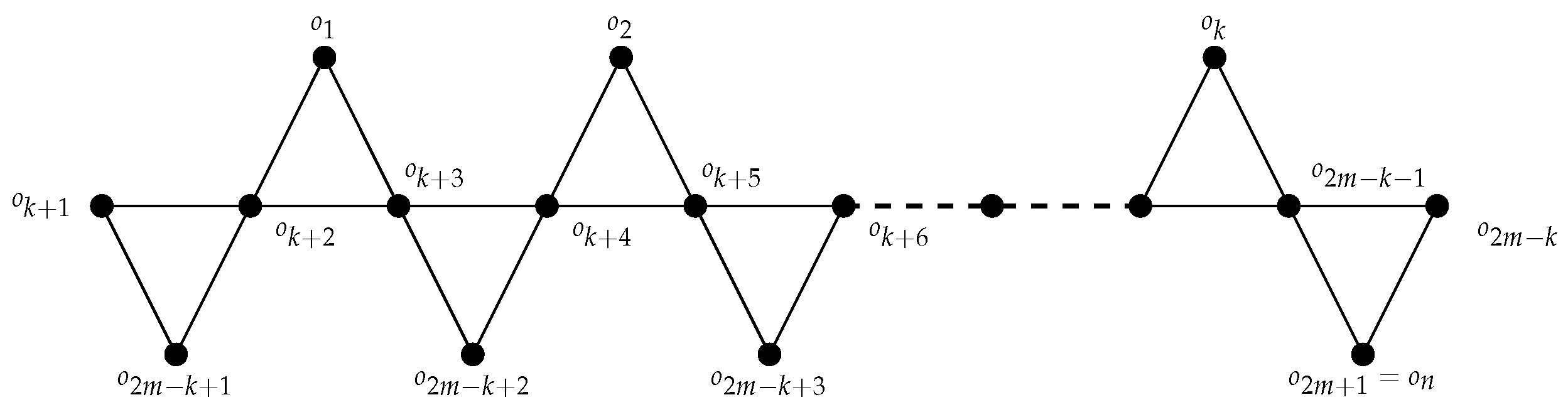
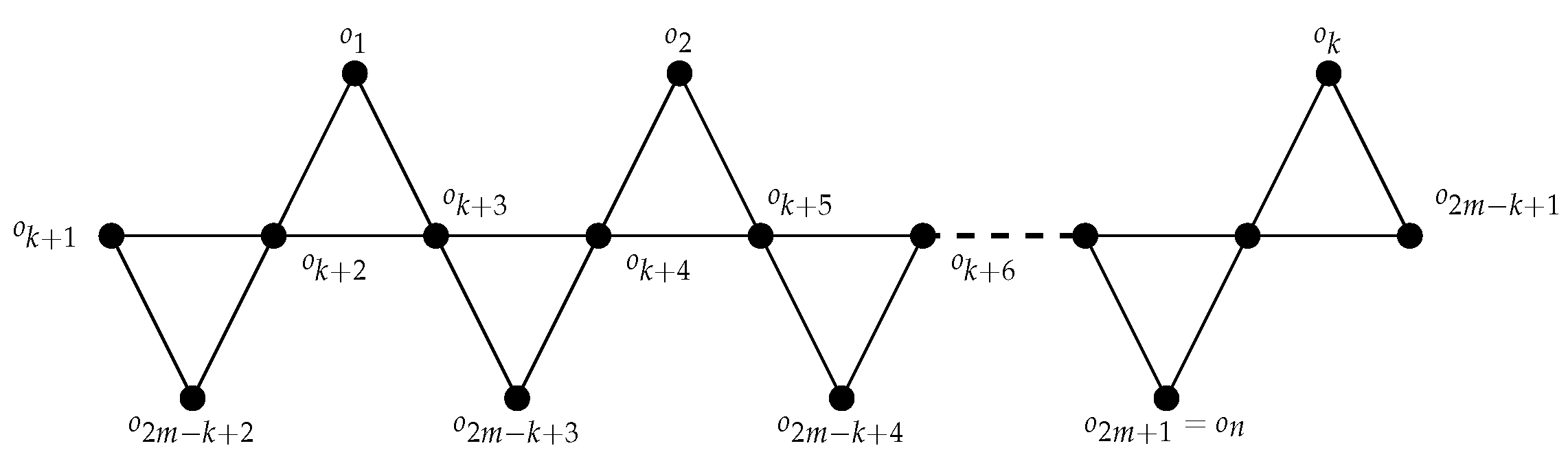
Consider the $SOXCN(1,m)$ interconnection networks with $2m+1$ nodes and $3m$ edges, where m is the number of edges in a row line. The graphs of $SOXCN$ with odd and even number m are shown in Figure 1 and Figure 2.

In the subsequent theorem, $pd\left(SOXCN\right(1,m\left)\right)$ is computed.

Theorem 3.

Consider $SOXCN(1,m)$ interconnection networks of order n with $n=2m+1$ for $m\ge 2$, then $pd\left(SOXCN\right(1,m\left)\right)=3$.

Proof. 

Let $\mathsf{\Lambda }=\{A_1,A_2,A_3\}$ be the partitioning set of $V\left(SOXCN\right(1,m\left)\right)$. The proof has two parts.

Case 1: 

When $n=2m+1$ with odd m and $k=\lfloor \frac{m}{2}\rfloor$, where m is the number of edges in a row line. Let $A_1=\left\{o_i\right|1\le i\le m+k\},A_2=\left\{o_{m+k+1}\right\}$ and $A_3=\left\{o_i\right|m+k+2\le i\le 2m+1=n\}$. The $r\left(o_i\right|\mathsf{\Lambda })$ are organized in Table 1.

Case 2: 

When $n=2m+1$ with even m and $k=\lfloor \frac{m}{2}\rfloor$, where m is the number of edges in a row line. Let $A_1=\left\{o_i\right|1\le i\le m+k-1\},A_2=\{o_{m+k},o_{m+k+1}\}$ and $A_3=\left\{o_i\right|m+k+2\le i\le 2m+1=n\}$. The $r\left(o_i\right|\mathsf{\Lambda })$ are organized in Table 2. It is easy to check from Table 1 and Table 2 that each representation is different. This implies that $pd\left(SOXCN\right(1,m\left)\right)\le 3$ and from Proposition 1 we conclude that, $pd\left(SOXCN\right(1,m\left)\right)=3$ for $m\ge 2$.

□

Table 1. $r\left(o_i\right|\mathsf{\Lambda })$ for $SOXCN(1,m)$ when $n=2m+1$ with odd m and $k=\lfloor \frac{m}{2}\rfloor$.

Nodes ${\mathit{o}}_{\mathit{i}}$	Distance from ${\mathit{A}}_1$	Distance from ${\mathit{A}}_2$	Distance from ${\mathit{A}}_3$
$1\le i\le k$	0	$m-2i+1$	2
$k+1\le i\le m+k$	0	$3k-i+2$	1
$i=m+k+1$	1	0	1
$m+k+2\le i\le 2m+1$	1	$4m-2i+3$	0

Table 1. $r\left(o_i\right|\mathsf{\Lambda })$ for $SOXCN(1,m)$ when $n=2m+1$ with odd m and $k=\lfloor \frac{m}{2}\rfloor$.

Nodes ${\mathit{o}}_{\mathit{i}}$	Distance from ${\mathit{A}}_1$	Distance from ${\mathit{A}}_2$	Distance from ${\mathit{A}}_3$
$1\le i\le k$	0	$m-2i+1$	2
$k+1\le i\le m+k$	0	$3k-i+2$	1
$i=m+k+1$	1	0	1
$m+k+2\le i\le 2m+1$	1	$4m-2i+3$	0

Table 2. $r\left(o_i\right|\mathsf{\Lambda })$ for $SOXCN(1,m)$ when $n=2m+1$ with even m and $k=\lfloor \frac{m}{2}\rfloor$.

Nodes ${\mathit{o}}_{\mathit{i}}$	Distance from ${\mathit{A}}_1$	Distance from ${\mathit{A}}_2$	Distance from ${\mathit{A}}_3$
$1\le i\le k-1$	0	$m-2i$	2
$i=k$	0	1	2
$k+1\le i\le m+k-1$	0	$3k-i$	1
$i=m+k$	1	0	1
$i=m+k+1$	1	0	2
$m+k+2\le i\le 2m+1$	1	$4m-2i+3$	0

Table 2. $r\left(o_i\right|\mathsf{\Lambda })$ for $SOXCN(1,m)$ when $n=2m+1$ with even m and $k=\lfloor \frac{m}{2}\rfloor$.

Nodes ${\mathit{o}}_{\mathit{i}}$	Distance from ${\mathit{A}}_1$	Distance from ${\mathit{A}}_2$	Distance from ${\mathit{A}}_3$
$1\le i\le k-1$	0	$m-2i$	2
$i=k$	0	1	2
$k+1\le i\le m+k-1$	0	$3k-i$	1
$i=m+k$	1	0	1
$i=m+k+1$	1	0	2
$m+k+2\le i\le 2m+1$	1	$4m-2i+3$	0

2.2. Partition Dimension of $RHOXN\left(n\right)$ Interconnection Networks

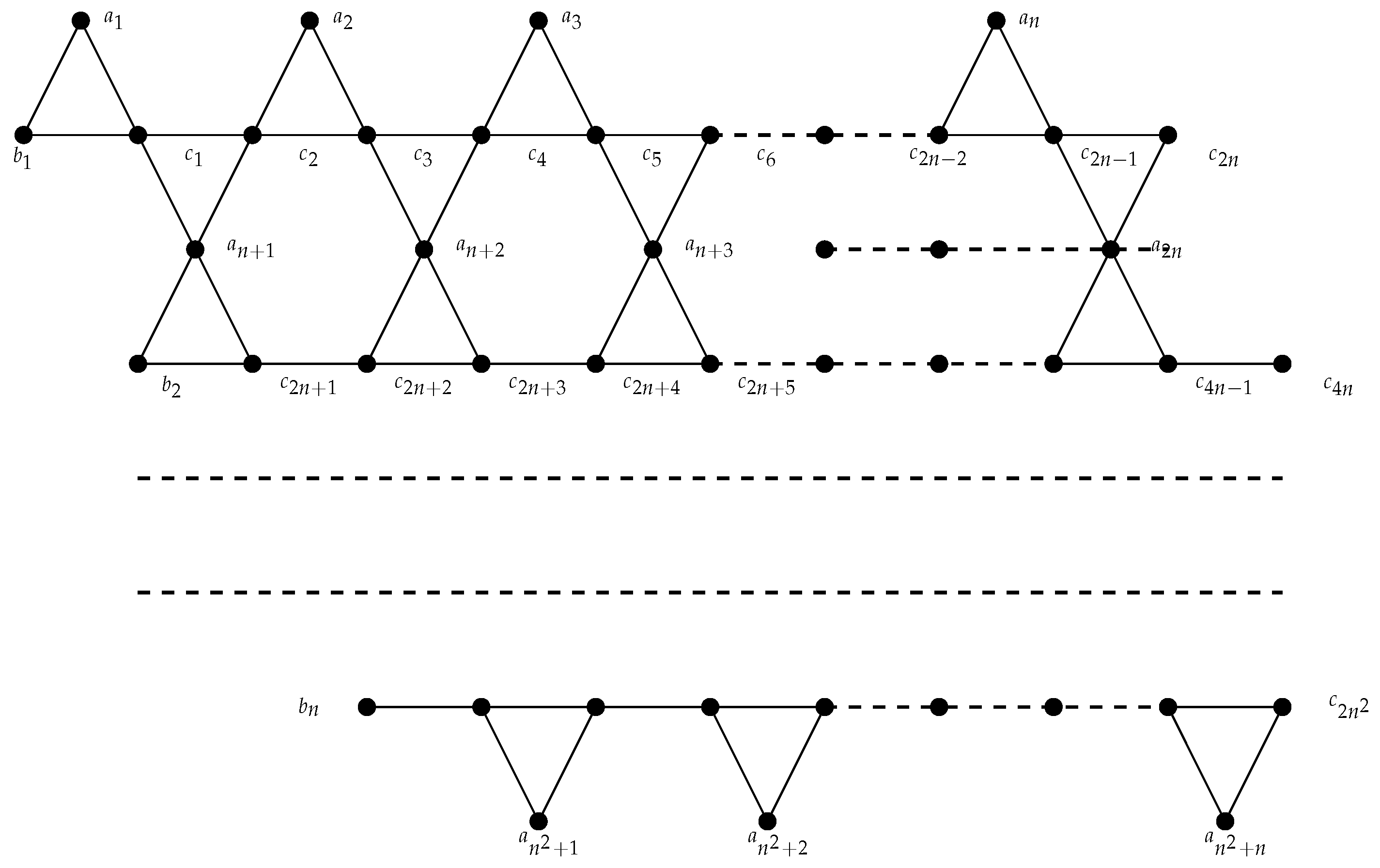
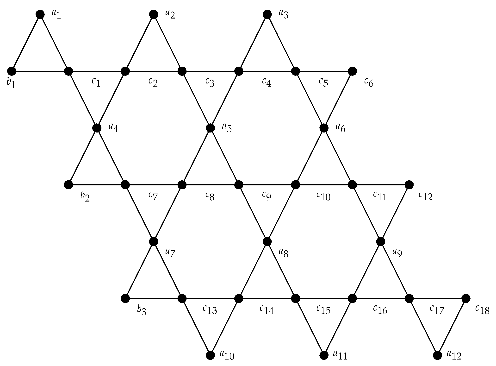
Consider the $RHOXN\left(n\right)$ interconnection networks of order $3n^2+2n$. The graph of $RHOXN\left(n\right)$ is shown in Figure 3 whereas Figure 4 elaborates the graph of $RHOXN\left(3\right)$.

In the subsequent theorem, $pd\left(RHOXN\right(n\left)\right)$ is computed.

Theorem 4.

Consider $RHOXN\left(n\right)$ interconnection networks of order $3n^2+2n$ for $n\ge 2$, then $pd\left(RHOXN\right(n\left)\right)=3$.

Proof. 

Assume that $\mathsf{\Lambda }=\{A_1,A_2,A_3\}$ be the partitioning set of $V\left(RHOXN\right(n\left)\right)$.

Let $A_1=\left\{a_i\right|1\le i\le n^2\}\cup \left\{c_i\right|1\le i\le 2n^2\},A_2=\left\{b_i\right|1\le i\le n\}$ and

$A_3=\left\{a_i\right|n^2+1\le i\le n^2+n\}$. The $r\left(a_i\right|\mathsf{\Lambda })$, $r\left(b_i\right|\mathsf{\Lambda })$ and $r\left(c_i\right|\mathsf{\Lambda })$ are organized in Table 3, Table 4 and Table 5, respectively.

It is easy to check from Table 3, Table 4 and Table 5 that each representation is different. This implies that $pd\left(RHOXN\right(n\left)\right)\le 3$ and from Proposition 1 we conclude that, $pd\left(RHOXN\right(n\left)\right)=3$ for $n\ge 2$. □

Table 3. $r\left(a_i\right|\mathsf{\Lambda })$ for $RHOXN\left(n\right)$.

Nodes ${\mathit{a}}_{\mathit{i}}$	Distance from ${\mathit{A}}_1$	Distance from ${\mathit{A}}_2$	Distance from ${\mathit{A}}_3$
$1\le i\le n$	0	$2i-1$	$2n$
$n+1\le i\le 2n$	0	$2(i-n)-1$	$2n-2$
$2n+1\le i\le 3n$	0	$2(i-2n)-1$	$2n-4$
⋮	⋮	⋮	⋮
$n^2-n+1\le i\le n^2$	0	$2(i-(n^2-n))-1$	2
$n^2+1\le i\le n^2+n$	1	$2(i-n^2)-1$	0

Table 3. $r\left(a_i\right|\mathsf{\Lambda })$ for $RHOXN\left(n\right)$.

Nodes ${\mathit{a}}_{\mathit{i}}$	Distance from ${\mathit{A}}_1$	Distance from ${\mathit{A}}_2$	Distance from ${\mathit{A}}_3$
$1\le i\le n$	0	$2i-1$	$2n$
$n+1\le i\le 2n$	0	$2(i-n)-1$	$2n-2$
$2n+1\le i\le 3n$	0	$2(i-2n)-1$	$2n-4$
⋮	⋮	⋮	⋮
$n^2-n+1\le i\le n^2$	0	$2(i-(n^2-n))-1$	2
$n^2+1\le i\le n^2+n$	1	$2(i-n^2)-1$	0

Table 4. $r\left(b_i\right|\mathsf{\Lambda })$ for $RHOXN\left(n\right)$.

Nodes ${\mathit{b}}_{\mathit{i}}$	Distance from ${\mathit{A}}_1$	Distance from ${\mathit{A}}_2$	Distance from ${\mathit{A}}_3$
$1\le i\le n$	1	0	$2n-2i+2$

Table 4. $r\left(b_i\right|\mathsf{\Lambda })$ for $RHOXN\left(n\right)$.

Nodes ${\mathit{b}}_{\mathit{i}}$	Distance from ${\mathit{A}}_1$	Distance from ${\mathit{A}}_2$	Distance from ${\mathit{A}}_3$
$1\le i\le n$	1	0	$2n-2i+2$

Table 5. $r\left(c_i\right|\mathsf{\Lambda })$ for $RHOXN\left(n\right)$.

Nodes ${\mathit{c}}_{\mathit{i}}$	Distance from ${\mathit{A}}_1$	Distance from ${\mathit{A}}_2$	Distance from ${\mathit{A}}_3$
$1\le i\le 2n$	0	i	$2n-1$
$2n+1\le i\le 4n$	0	$i-2n$	$2n-3$
$4n+1\le i\le 6n$	0	$i-4n$	$2n-5$
⋮	⋮	⋮	⋮
$2n^2-2n+1\le i\le 2n^2$	0	$i-(2n^2-2n)$	1

Table 5. $r\left(c_i\right|\mathsf{\Lambda })$ for $RHOXN\left(n\right)$.

Nodes ${\mathit{c}}_{\mathit{i}}$	Distance from ${\mathit{A}}_1$	Distance from ${\mathit{A}}_2$	Distance from ${\mathit{A}}_3$
$1\le i\le 2n$	0	i	$2n-1$
$2n+1\le i\le 4n$	0	$i-2n$	$2n-3$
$4n+1\le i\le 6n$	0	$i-4n$	$2n-5$
⋮	⋮	⋮	⋮
$2n^2-2n+1\le i\le 2n^2$	0	$i-(2n^2-2n)$	1

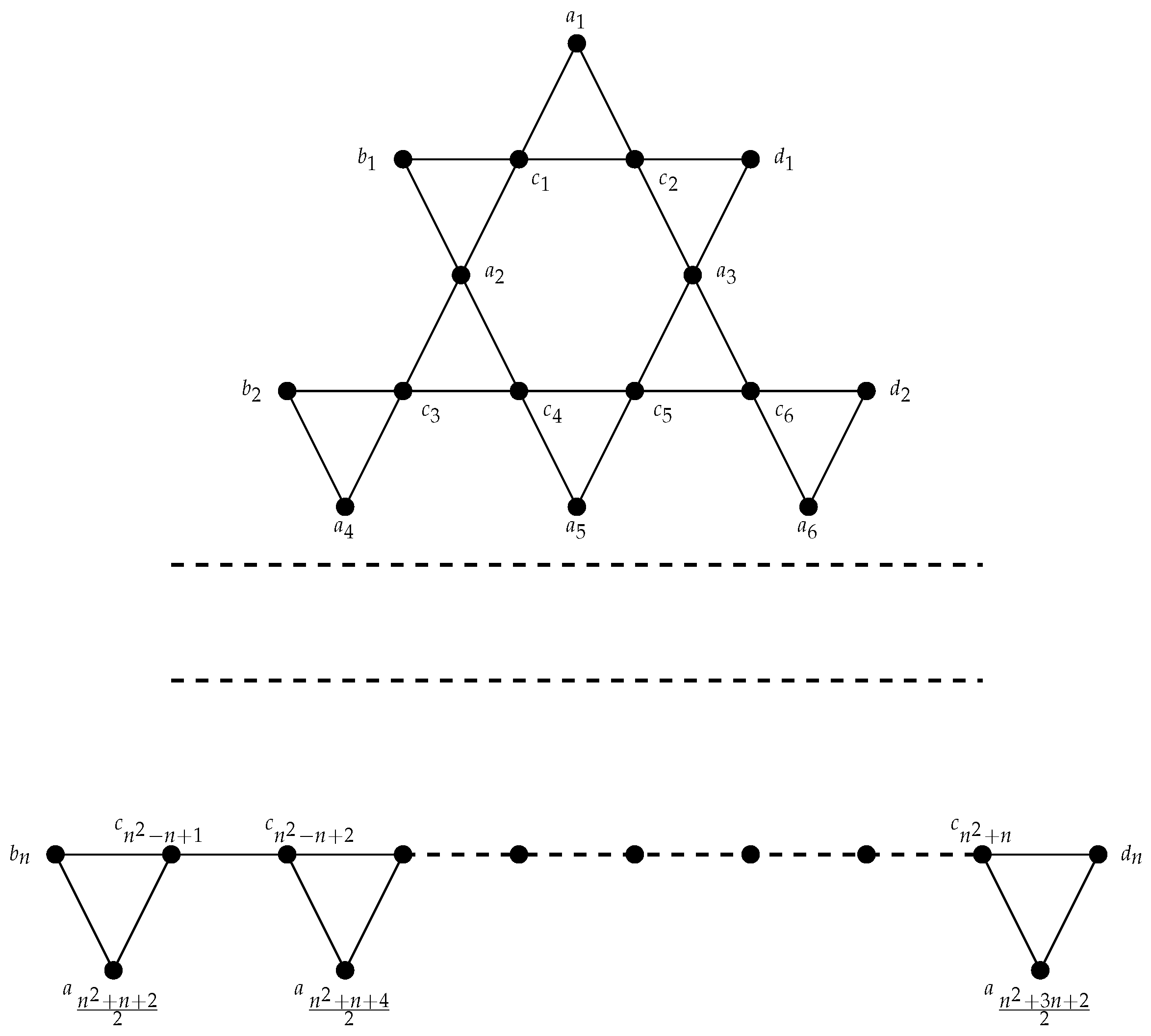
2.3. Partition Dimension of $RTOXN\left(n\right)$ Interconnection Networks

Consider the $RTOXN\left(n\right)$ interconnection networks of order $\frac{3n^2+9n+2}{2}$. The graph of $RTOXN\left(n\right)$ is shown in Figure 5.

Theorem 5.

Consider $RTOXN\left(n\right)$ interconnection networks of order $\frac{3n^2+9n+2}{2}$ for $n\ge 2$, then $pd\left(RTOXN\right(n\left)\right)=3$.

Proof. 

Assume that $\mathsf{\Lambda }=\{A_1,A_2,A_3\}$ be the partitioning set of $V\left(RTOXN\right(n\left)\right)$.

Let $A_1=\left\{a_i\right|1\le i\le \frac{n^2+n}{2}\}\cup \left\{c_i\right|1\le i\le n^2+n\}\cup \left\{d_i\right|1\le i\le n\},A_2=\left\{b_i\right|1\le i\le n\}$ and $A_3=\left\{a_i\right|\frac{n^2+n+2}{2}\le i\le \frac{n^2+3n+2}{2}\}$.

The $r\left(a_i\right|\mathsf{\Lambda })$, $r\left(b_i\right|\mathsf{\Lambda })$, $r\left(c_i\right|\mathsf{\Lambda })$ and $r\left(d_i\right|\mathsf{\Lambda })$ are organized in Table 6, Table 7, Table 8 and Table 9, respectively.

It is easy to check from Table 6, Table 7, Table 8 and Table 9 that each representation is different. This implies that $pd\left(RTOXN\right(n\left)\right)\le 3$ and from Proposition 1 we conclude that, $pd\left(RTOXN\right(n\left)\right)=3$ for $n\ge 2$. □

Table 6. $r\left(a_i\right|\mathsf{\Lambda })$ for $RTOXN$.

Nodes ${\mathit{a}}_{\mathit{i}}$	Distance from ${\mathit{A}}_1$	Distance from ${\mathit{A}}_2$	Distance from ${\mathit{A}}_3$
$i=1$	0	2	$2n$
$2\le i\le 3$	0	$2i-{\alpha }_0,{\alpha }_0=3$	$2(n-1)$
$4\le i\le 6$	0	$2i-{\alpha }_1$	$2(n-2)$
$7\le i\le 10$	0	$2i-{\alpha }_2$	$2(n-3)$
⋮	⋮	⋮	⋮
$\frac{n^2-n+2}{2}\le i\le \frac{n^2+n}{2}$	0	$2i-{\alpha }_{n-2}$	2
$\frac{n^2+n+2}{2}\le i\le \frac{n^2+3n+2}{2}$	1	$2i-{\alpha }_{n-1}$	0
		${\alpha }_k=k^2+3k+3$

Table 6. $r\left(a_i\right|\mathsf{\Lambda })$ for $RTOXN$.

Nodes ${\mathit{a}}_{\mathit{i}}$	Distance from ${\mathit{A}}_1$	Distance from ${\mathit{A}}_2$	Distance from ${\mathit{A}}_3$
$i=1$	0	2	$2n$
$2\le i\le 3$	0	$2i-{\alpha }_0,{\alpha }_0=3$	$2(n-1)$
$4\le i\le 6$	0	$2i-{\alpha }_1$	$2(n-2)$
$7\le i\le 10$	0	$2i-{\alpha }_2$	$2(n-3)$
⋮	⋮	⋮	⋮
$\frac{n^2-n+2}{2}\le i\le \frac{n^2+n}{2}$	0	$2i-{\alpha }_{n-2}$	2
$\frac{n^2+n+2}{2}\le i\le \frac{n^2+3n+2}{2}$	1	$2i-{\alpha }_{n-1}$	0
		${\alpha }_k=k^2+3k+3$

Table 7. $r\left(b_i\right|\mathsf{\Lambda })$ for $RTOXN$.

Nodes ${\mathit{b}}_{\mathit{i}}$	Distance from ${\mathit{A}}_1$	Distance from ${\mathit{A}}_2$	Distance from ${\mathit{A}}_3$
$1\le i\le n$	1	0	$2n-2i+1$

Table 7. $r\left(b_i\right|\mathsf{\Lambda })$ for $RTOXN$.

Nodes ${\mathit{b}}_{\mathit{i}}$	Distance from ${\mathit{A}}_1$	Distance from ${\mathit{A}}_2$	Distance from ${\mathit{A}}_3$
$1\le i\le n$	1	0	$2n-2i+1$

Table 8. $r\left(c_i\right|\mathsf{\Lambda })$ for $RTOXN$.

Nodes ${\mathit{c}}_{\mathit{i}}$	Distance from ${\mathit{A}}_1$	Distance from ${\mathit{A}}_2$	Distance from ${\mathit{A}}_3$
$1\le i\le 2$	0	i	$2n-1$
$3\le i\le 6$	0	$i-{\gamma }_0,{\gamma }_0=2$	$2n-3$
$7\le i\le 12$	0	$i-{\gamma }_1$	$2n-5$
⋮	⋮	⋮	⋮
$n^2-3n+3\le i\le n^2-n$	0	$i-{\gamma }_{n-3}$	3
$n^2-n+1\le i\le n^2+n$	0	$i-{\gamma }_{n-2}$	1
		${\gamma }_k=k^2+3k+2$

Table 8. $r\left(c_i\right|\mathsf{\Lambda })$ for $RTOXN$.

Nodes ${\mathit{c}}_{\mathit{i}}$	Distance from ${\mathit{A}}_1$	Distance from ${\mathit{A}}_2$	Distance from ${\mathit{A}}_3$
$1\le i\le 2$	0	i	$2n-1$
$3\le i\le 6$	0	$i-{\gamma }_0,{\gamma }_0=2$	$2n-3$
$7\le i\le 12$	0	$i-{\gamma }_1$	$2n-5$
⋮	⋮	⋮	⋮
$n^2-3n+3\le i\le n^2-n$	0	$i-{\gamma }_{n-3}$	3
$n^2-n+1\le i\le n^2+n$	0	$i-{\gamma }_{n-2}$	1
		${\gamma }_k=k^2+3k+2$

Table 9. $r\left(d_i\right|\mathsf{\Lambda })$ for $RTOXN$.

Nodes ${\mathit{d}}_{\mathit{i}}$	Distance from ${\mathit{A}}_1$	Distance from ${\mathit{A}}_2$	Distance from ${\mathit{A}}_3$
$1\le i\le n$	0	$2i+1$	$2n-2i+1$

Table 9. $r\left(d_i\right|\mathsf{\Lambda })$ for $RTOXN$.

Nodes ${\mathit{d}}_{\mathit{i}}$	Distance from ${\mathit{A}}_1$	Distance from ${\mathit{A}}_2$	Distance from ${\mathit{A}}_3$
$1\le i\le n$	0	$2i+1$	$2n-2i+1$

3. Fault Tolerant Partition Dimension of Interconnection Networks

In the forthcoming subsections, the fault tolerant partition dimension of $SOXCN$, $RHOXN$ and $RTOXN$ interconnection networks is computed.

3.1. Fault Tolerant Partition Dimension of $SOXCN(1,m)$ Interconnection Networks

In the subsequent theorem, $p{d}_2\left(SOXCN(1,m)\right)$ is computed.

Theorem 6.

Consider $SOXCN(1,m)$ interconnection networks of order n with $n=2m+1$ for $m\ge 2$, then $p{d}_2\left(SOXCN(1,m)\right)=4$.

Proof. 

Let $\mathsf{\Lambda }=\{A_1,A_2,A_3,A_4\}$ be the partitioning set of $V\left(SOXCN\right(1,m\left)\right)$. The proof has two parts.

Case 1: 

When $n=2m+1$ with odd m and $k=\lfloor \frac{m}{2}\rfloor$, where m is the number of edges in a row line. Let $A_1=\left\{o_i\right|1\le i\le k\}\cup \left\{o_i\right|k+3\le i\le 2m-k-2\},A_2=\{o_{k+1},o_{k+2}\}$, $A_3=\{o_{2m-k-1},o_{2m-k}\}$ and $A_4=\left\{o_i\right|2m-k+1\le i\le 2m+1=n\}$. The $r\left(o_i\right|\mathsf{\Lambda })$ are organized in Table 10.

Case 2: 

When $n=2m+1$ with even m and $k=\lfloor \frac{m}{2}\rfloor$, where m is the number of edges in a row line. Let $A_1=\left\{o_i\right|1\le i\le k\}\cup \left\{o_i\right|k+3\le i\le 2m-k-1\},A_2=\{o_{k+1},o_{k+2}\}$, $A_3=\{o_{2m-k},o_{2m-k+1}\}$ and $A_4=\left\{o_i\right|2m-k+2\le i\le 2m+1=n\}$. The $r\left(o_i\right|\mathsf{\Lambda })$ are organized in Table 11.

Table 10 to Table 11 obviously prove that $\mathsf{\Lambda }$ is a $2-$ resolving generator of $SOXCN(1,m)$ for $m\ge 2$, therefore, $p{d}_2\left(OX(1,m)\right)\le 4$ for $m\ge 2$. Lemma 2 implies that $p{d}_2\left(SOXCN(1,m)\right)\ge 4$ for $m\ge 2$. This establishes our assertion.

□

Table 10. Fault tolerant partition representations of nodes $o_i$ for $SOXCN(1,m)$ when $n=2m+1$ with odd m and $k=\lfloor \frac{m}{2}\rfloor$.

Nodes ${\mathit{o}}_{\mathit{i}}$	Distance from ${\mathit{A}}_1$	Distance from ${\mathit{A}}_2$	Distance from ${\mathit{A}}_3$	Distance from ${\mathit{A}}_4$
$1\le i\le k$	0	$2i-1$	$m-2i$	2
$k+3\le i\le 2m-k-2$	0	$i-k-2$	$3k-i+1$	1
$i=k+1$	2	0	$m-1$	1
$i=k+2$	1	0	$m-2$	1
$i=2m-k-1$	1	$m-2$	0	1
$i=2m-k$	2	$m-1$	0	1
$i=2m-k+1$	2	1	$m-1$	0
$2m-k+2\le i\le 2m$	1	$2i-3m-3$	$4m-2i+2$	0
$i=2m+1$	2	$m-1$	1	0

Table 10. Fault tolerant partition representations of nodes $o_i$ for $SOXCN(1,m)$ when $n=2m+1$ with odd m and $k=\lfloor \frac{m}{2}\rfloor$.

Nodes ${\mathit{o}}_{\mathit{i}}$	Distance from ${\mathit{A}}_1$	Distance from ${\mathit{A}}_2$	Distance from ${\mathit{A}}_3$	Distance from ${\mathit{A}}_4$
$1\le i\le k$	0	$2i-1$	$m-2i$	2
$k+3\le i\le 2m-k-2$	0	$i-k-2$	$3k-i+1$	1
$i=k+1$	2	0	$m-1$	1
$i=k+2$	1	0	$m-2$	1
$i=2m-k-1$	1	$m-2$	0	1
$i=2m-k$	2	$m-1$	0	1
$i=2m-k+1$	2	1	$m-1$	0
$2m-k+2\le i\le 2m$	1	$2i-3m-3$	$4m-2i+2$	0
$i=2m+1$	2	$m-1$	1	0

Table 11. Fault tolerant partition representations of nodes $o_i$ for $SOXCN(1,m)$ when $n=2m+1$ with even m and $k=\lfloor \frac{m}{2}\rfloor$.

Nodes ${\mathit{o}}_{\mathit{i}}$	Distance from ${\mathit{A}}_1$	Distance from ${\mathit{A}}_2$	Distance from ${\mathit{A}}_3$	Distance from ${\mathit{A}}_4$
$1\le i\le k-1$	0	$2i-1$	$m-2i$	2
$i=k$	0	$m-1$	1	2
$k+3\le i\le 2m-k-1$	0	$i-k-2$	$3k-i$	1
$i=k+1$	2	0	$m-1$	1
$i=k+2$	1	0	$m-2$	1
$i=2m-k$	1	$m-2$	0	1
$i=2m-k+1$	1	$m-1$	0	2
$i=2m-k+2$	2	1	$m-1$	0
$2m-k+3\le i\le 2m+1$	1	$2i-3m-4$	$4m-2i+3$	0

Table 11. Fault tolerant partition representations of nodes $o_i$ for $SOXCN(1,m)$ when $n=2m+1$ with even m and $k=\lfloor \frac{m}{2}\rfloor$.

Nodes ${\mathit{o}}_{\mathit{i}}$	Distance from ${\mathit{A}}_1$	Distance from ${\mathit{A}}_2$	Distance from ${\mathit{A}}_3$	Distance from ${\mathit{A}}_4$
$1\le i\le k-1$	0	$2i-1$	$m-2i$	2
$i=k$	0	$m-1$	1	2
$k+3\le i\le 2m-k-1$	0	$i-k-2$	$3k-i$	1
$i=k+1$	2	0	$m-1$	1
$i=k+2$	1	0	$m-2$	1
$i=2m-k$	1	$m-2$	0	1
$i=2m-k+1$	1	$m-1$	0	2
$i=2m-k+2$	2	1	$m-1$	0
$2m-k+3\le i\le 2m+1$	1	$2i-3m-4$	$4m-2i+3$	0

3.2. Fault Tolerant Partition Dimension of $RHOXN\left(n\right)$ Interconnection Networks

In the forthcoming result, $p{d}_2\left(RHOXN\left(n\right)\right)$ is computed.

Theorem 7.

Consider $RHOXN\left(n\right)$ interconnection networks of order $3n^2+2n$ for $n\ge 2$, then $p{d}_2\left(RHOXN\left(n\right)\right)=4$.

Proof. 

Assume that $\mathsf{\Lambda }=\{A_1,A_2,A_3,A_4\}$ be the partitioning set of $V\left(RHOXN\right(n\left)\right)$.

Let $A_1=\left\{a_i\right|1\le i\le n^2\}\cup \left\{b_i\right|2\le i\le n\}\cup \left\{c_i\right|c_i\notin A_3\},A_2=\left\{b_1\right\}$, $A_3=\left\{c_{2ni}\right|1\le i\le n\}$ and $A_4=\left\{a_i\right|n^2+1\le i\le n^2+n\}$. The $r\left(a_i\right|\mathsf{\Lambda })$, $r\left(b_i\right|\mathsf{\Lambda })$ and $r\left(c_i\right|\mathsf{\Lambda })$ are organized in Table 12, Table 13 and Table 14, respectively. Table 12 to Table 14 obviously prove that $\mathsf{\Lambda }$ is a $2-$ resolving generator of $RHOXN\left(n\right)$ for $n\ge 2$ so we have, $p{d}_2\left(RHOXN\left(n\right)\right)\le 4$ for $n\ge 2$. Lemma 2 infers that $p{d}_2\left(RHOXN\left(n\right)\right)\ge 4$ for $n\ge 2$. This confirms our assertion.

□

Table 12. Fault tolerant partition representations of nodes $a_i$ for $RHOXN$.

Nodes ${\mathit{a}}_{\mathit{i}}$	Distance from ${\mathit{A}}_1$	Distance from ${\mathit{A}}_2$	Distance from ${\mathit{A}}_3$	Distance from ${\mathit{A}}_4$
$1\le i\le n$	0	$2i-1$	$2n-2i+2$	$2n$
$n+1\le i\le 2n$	0	$2(i-n)$	$4n-2i+1$	$2n-2$
$2n+1\le i\le 3n$	0	$2(i-2n)+2$	$6n-2i+1$	$2n-4$
$3n+1\le i\le 4n$	0	$2(i-3n)+4$	$8n-2i+1$	$2n-6$
⋮	⋮	⋮	⋮	⋮
$n^2-n+1\le i\le n^2$	0	$2(i-(n^2-n))+2(n-2)$	$2n^2-2i+1$	2
$n^2+1\le i\le n^2+n$	1	$2(i-(n^2+1))+2n$	$2n^2+2n-2i+1$	0

Table 12. Fault tolerant partition representations of nodes $a_i$ for $RHOXN$.

Nodes ${\mathit{a}}_{\mathit{i}}$	Distance from ${\mathit{A}}_1$	Distance from ${\mathit{A}}_2$	Distance from ${\mathit{A}}_3$	Distance from ${\mathit{A}}_4$
$1\le i\le n$	0	$2i-1$	$2n-2i+2$	$2n$
$n+1\le i\le 2n$	0	$2(i-n)$	$4n-2i+1$	$2n-2$
$2n+1\le i\le 3n$	0	$2(i-2n)+2$	$6n-2i+1$	$2n-4$
$3n+1\le i\le 4n$	0	$2(i-3n)+4$	$8n-2i+1$	$2n-6$
⋮	⋮	⋮	⋮	⋮
$n^2-n+1\le i\le n^2$	0	$2(i-(n^2-n))+2(n-2)$	$2n^2-2i+1$	2
$n^2+1\le i\le n^2+n$	1	$2(i-(n^2+1))+2n$	$2n^2+2n-2i+1$	0

Table 13. Fault tolerant partition representations of nodes $b_i$ for $RHOXN$.

Nodes ${\mathit{b}}_{\mathit{i}}$	Distance from ${\mathit{A}}_1$	Distance from ${\mathit{A}}_2$	Distance from ${\mathit{A}}_3$	Distance from ${\mathit{A}}_4$
$i=1$	1	0	$2n$	$2n$
$2\le i\le n$	0	$2i-1$	$2n$	$2n-2i+2$

Table 13. Fault tolerant partition representations of nodes $b_i$ for $RHOXN$.

Nodes ${\mathit{b}}_{\mathit{i}}$	Distance from ${\mathit{A}}_1$	Distance from ${\mathit{A}}_2$	Distance from ${\mathit{A}}_3$	Distance from ${\mathit{A}}_4$
$i=1$	1	0	$2n$	$2n$
$2\le i\le n$	0	$2i-1$	$2n$	$2n-2i+2$

Table 14. Fault tolerant partition representations of nodes $c_i$ for $RHOXN$.

Nodes ${\mathit{c}}_{\mathit{i}}$	Distance from ${\mathit{A}}_1$	Distance from ${\mathit{A}}_2$	Distance from ${\mathit{A}}_3$	Distance from ${\mathit{A}}_4$
$c_{2ni}$($1\le i\le n$)	1	$2n+2i-2$	0	$2n-2i+1$
$c_i$($1\le i\le 2n-1$)	0	i	$2n-i$	$2n-1$
$c_{i+2n}$($1\le i\le 2n-1$ )	0	$i+2$	$2n-i$	$2n-3$
$c_{i+4n}$($1\le i\le 2n-1$)	0	$i+4$	$2n-i$	$2n-5$
$c_{i+6n}$($1\le i\le 2n-1$)	0	$i+6$	$2n-i$	$2n-7$
⋮	⋮	⋮	⋮	⋮
$c_{i+2n^2-2n}$($1\le i\le 2n-1$)	0	$i+2n-2$	$2n-i$	1

Table 14. Fault tolerant partition representations of nodes $c_i$ for $RHOXN$.

Nodes ${\mathit{c}}_{\mathit{i}}$	Distance from ${\mathit{A}}_1$	Distance from ${\mathit{A}}_2$	Distance from ${\mathit{A}}_3$	Distance from ${\mathit{A}}_4$
$c_{2ni}$($1\le i\le n$)	1	$2n+2i-2$	0	$2n-2i+1$
$c_i$($1\le i\le 2n-1$)	0	i	$2n-i$	$2n-1$
$c_{i+2n}$($1\le i\le 2n-1$ )	0	$i+2$	$2n-i$	$2n-3$
$c_{i+4n}$($1\le i\le 2n-1$)	0	$i+4$	$2n-i$	$2n-5$
$c_{i+6n}$($1\le i\le 2n-1$)	0	$i+6$	$2n-i$	$2n-7$
⋮	⋮	⋮	⋮	⋮
$c_{i+2n^2-2n}$($1\le i\le 2n-1$)	0	$i+2n-2$	$2n-i$	1

3.3. Fault Tolerant Partition Dimension of $RTOXN\left(n\right)$ Interconnection Networks

In the following theorem, $p{d}_2\left(RTOXN\left(n\right)\right)$ is computed.

Theorem 8.

Consider $RTOXN\left(n\right)$ interconnection networks of order $\frac{3n^2+9n+2}{2}$ for $n\ge 2$, then $p{d}_2\left(RTOXN\left(n\right)\right)=4$.

Proof. 

Assume that $\mathsf{\Lambda }=\{A_1,A_2,A_3,A_4\}$ be the partitioning set of $V\left(RTOXN\right(n\left)\right)$.

Let $A_1=\left\{a_i\right|1\le i\le \frac{n^2+n}{2}\}\cup \left\{c_i\right|1\le i\le n^2+n\},A_2=\left\{b_i\right|1\le i\le n\}$, $A_3=\left\{d_i\right|1\le i\le n\}$ and $A_4=\left\{a_i\right|\frac{n^2+n+2}{2}\le i\le \frac{n^2+3n+2}{2}\}$. The $r\left(a_i\right|\mathsf{\Lambda })$, $r\left(b_i\right|\mathsf{\Lambda })$, $r\left(c_i\right|\mathsf{\Lambda })$ and $r\left(d_i\right|\mathsf{\Lambda })$ are organized in

Table 15. Fault tolerant partition representations of nodes $a_i$ for $RTOXN$.

Nodes ${\mathit{a}}_{\mathit{i}}$	Distance from ${\mathit{A}}_1$	Distance from ${\mathit{A}}_2$	Distance from ${\mathit{A}}_3$	Distance from ${\mathit{A}}_4$
$i=1$	0	2	2	$2n$
$2\le i\le 3$	0	$2i-{\alpha }_0,{\alpha }_0=3$	${\beta }_0-2i,{\beta }_0=7$	$2(n-1)$
$4\le i\le 6$	0	$2i-{\alpha }_1$	${\beta }_1-2i$	$2(n-2)$
$7\le i\le 10$	0	$2i-{\alpha }_2$	${\beta }_2-2i$	$2(n-3)$
⋮	⋮	⋮	⋮	⋮
$\frac{n^2-n+2}{2}\le i\le \frac{n^2+n}{2}$	0	$2i-{\alpha }_{n-2}$	${\beta }_{n-2}-2i$	2
$\frac{n^2+n+2}{2}\le i\le \frac{n^2+3n+2}{2}$	1	$2i-{\alpha }_{n-1}$	${\beta }_{n-1}-2i$	0
		${\alpha }_k=k^2+3k+3$	${\beta }_k=k^2+5k+7$

,

Table 16. Fault tolerant partition representations of nodes $b_i$ for $RTOXN$.

Nodes ${\mathit{b}}_{\mathit{i}}$	Distance from ${\mathit{A}}_1$	Distance from ${\mathit{A}}_2$	Distance from ${\mathit{A}}_3$	Distance from ${\mathit{A}}_4$
$1\le i\le n$	1	0	$2i+1$	$2n-2i+1$

,

Table 17. Fault tolerant partition representations of nodes $c_i$ for $RTOXN$.

Nodes ${\mathit{c}}_{\mathit{i}}$	Distance from ${\mathit{A}}_1$	Distance from ${\mathit{A}}_2$	Distance from ${\mathit{A}}_3$	Distance from ${\mathit{A}}_4$
$1\le i\le 2$	0	i	$3-i$	$2n-1$
$3\le i\le 6$	0	$i-{\gamma }_0,{\gamma }_0=2$	${\beta }_0-i,{\beta }_0=7$	$2n-3$
$7\le i\le 12$	0	$i-{\gamma }_1$	${\beta }_1-i$	$2n-5$
⋮	⋮	⋮	⋮	⋮
$n^2-3n+3\le i\le n^2-n$	0	$i-{\gamma }_{n-3}$	${\beta }_{n-3}-i$	3
$n^2-n+1\le i\le n^2+n$	0	$i-{\gamma }_{n-2}$	${\beta }_{n-2}-i$	1
		${\gamma }_k=k^2+3k+2$	${\beta }_k=k^2+5k+7$

and

Table 18. Fault tolerant partition representations of nodes $d_i$ for $RTOXN$.

Nodes ${\mathit{d}}_{\mathit{i}}$	Distance from ${\mathit{A}}_1$	Distance from ${\mathit{A}}_2$	Distance from ${\mathit{A}}_3$	Distance from ${\mathit{A}}_4$
$1\le i\le n$	1	$2i+1$	0	$2n-2i+1$

, respectively. Table 15 to Table 18 obviously prove that $\mathsf{\Lambda }$ is a $2-$ resolving generator of $RTOXN\left(n\right)$ for $n\ge 2$ so we have, $p{d}_2\left(RTOXN\left(n\right)\right)\le 4$ for $n\ge 2$. Lemma 2 infers that $p{d}_2\left(RTOXN\left(n\right)\right)\ge 4$ for $n\ge 2$. This confirms our assertion. □

4. Application

The applications of partition and fault tolerant addressing schemes have recently been discussed for routing optimization in [29], supply chain optimization in [31] and sensors deployment in [6]. In this section, an application of the fault tolerant addressing scheme in the context of optimal data flow is included.

The performance of a network depends on the network topology and routing algorithm. Unique addressing schemes have been proposed in the literature for the interconnection networks for efficient routing. One way to assign unique addresses to nodes of the networks is to distribute nodes into different regions or subnets which allows efficient implementation of routing algorithms and also reduces the size of routing tables (see [4,5]). In this context, resolving partitions divide nodes into subnets and assign unique addresses to all the nodes in terms of distances from the subnets. A fault tolerant partition generator works in the presence of fault as if one of the subnets is not accessible then other subnets can still uniquely identify the nodes in terms of distances from the remaining subnets. We can choose suitable sizes for both resolving partitions and fault tolerant partition generators according to our needs but attaining the minimal size is NP-hard for general networks see [33].

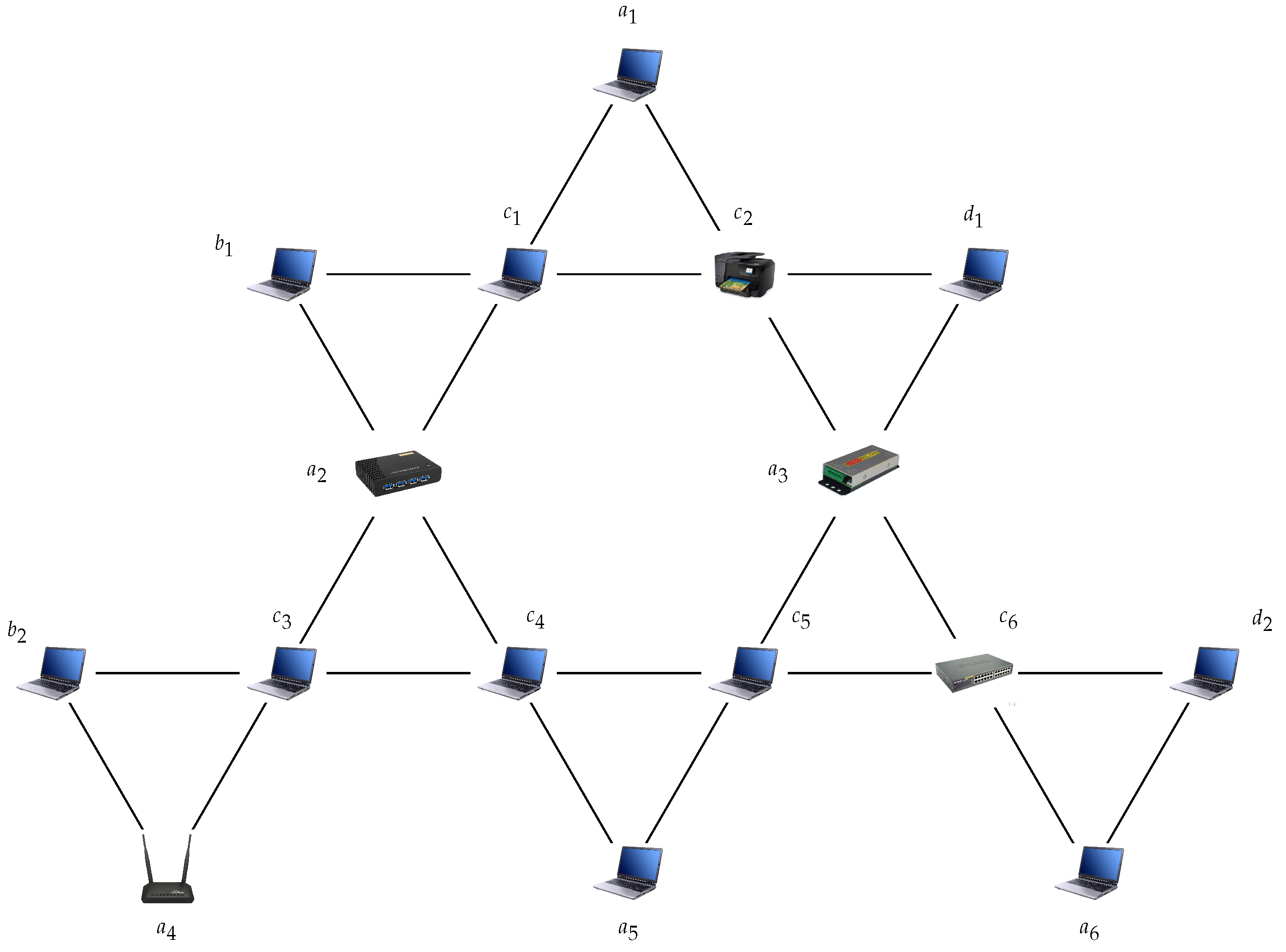
An interconnection network is equipped with many devices such as laptops, printers, switches, repeaters, routers, bridges and hubs. The aim is to overcome memory requirements, delays in data transfer and power consumption which increase with the increasing size of networks. As an explanatory case, consider an interconnection network in the form of $RTOXN\left(2\right)$ in Figure 6, the devices are nodes and connections among these are edges of the network. We can split Figure 6 into 3 and 4 four regions according to Theorem 2.3 and Theorem 3.4, respectively. The 3 and 4 - dimensional unique addresses can be constructed from the tables given in these theorems.

Fault tolerant basis for $RTOXN\left(2\right)$: $A_1=\{a_1,a_2,a_3,c_1,c_2,c_3,c_4,c_5,c_6\}$, $A_2=\{b_1,b_2\}$,

$A_3=\{d_1,d_2\},A_4=\{a_4,a_5,a_6\}.$

4—dimensional fault tolerant addresses for $RTOXN\left(2\right)$:

$a_1(0,2,2,4),c_1(0,1,2,3)$, $c_2(0,2,1,3),a_2(0,1,3,2),$$a_3(0,3,1,2),c_3(0,1,4,1),c_4(0,2,3,1),$$c_5(0,3,2,1)$, $c_6(0,4,1,1),b_1(1,0,3,3),b_2(1,0,5,1)$, $d_1(1,3,0,3),d_2(1,5,0,1),a_4(1,1,5,0)$, $a_5(1,3,3,0),a_6(1,5,1,0).$

It is evident from the addresses of nodes that the whole network is split into four regions and addresses are unique in at least two places which can reduce the routing tables considerably and can improve the efficiency of routing and broadcasting algorithms. Suppose in Figure 6 if we want to pass the message from $c_1$ to $a_3$ which are in the same region then we can follow the path $c_1-c_2-a_3$ but if the connection between $c_2$ and $a_3$ is faulty then $c_2$ can pass the message to $d_1$ which is in the other region and can pass message to $a_3$.

5. Conclusions

In this manuscript, the partition and fault tolerant partition dimension of $SOXCN$, $RHOXN$ and $RTOXN$ interconnection networks, are computed. It is shown that these metric-related parameters have constant values for these networks and do not depend on the order of the network. The computed parameters can be used to assign unique addresses to processing nodes which can help to attain efficient routing and broadcasting in a network. The fact that computing partition and fault tolerant partition dimension for any network is NP hard see [33], provides challenges in this domain. In the mean time, this also provides the scope for computing these parameters on different classes of graphs depending on their symmetric behavior. In the end, we propose an open problem.

Open Problem 9. 

Find the partition and fault tolerant partition dimensions of dominating silicate networks and dominating oxide networks.

References

- Chen, M.S.; Shin, K.G.; Kandlur, D.D. Addressing, routing, and broadcasting in hexagonal mesh multiprocessors. IEEE Trans Comput. 1990, 39, 10–18. [Google Scholar] [CrossRef] [Green Version]
- Olson, A.; Shin, K.G. Fault tolerant routing in mesh architectures. IEEE Trans. Parallel Distrib. Syst. 1994, 5, 1225–1232. [Google Scholar] [CrossRef] [Green Version]
- García, F.; Solano, J.; Stojmenovic, I.; Stojmenovic, M. Higher dimensional hexagonal networks. J. Parallel Distrib. Comput. 2003, 63, 1164–1172. [Google Scholar] [CrossRef]
- Mejia, A.; Flich, J.; Reinemo, S.A.; Skeie, T. Segment-based routing: An efficient fault-tolerant routing algorithm for meshes and tori. In Proceedings of the 20th IEEE International Parallel & Distributed Processing Symposium, Rhodes, Greece, 25–29 April 2006; pp. 1–10. [Google Scholar]
- Mejia, A.; Palesi, M.; Flich, J.; Kumar, S.; Lopez, P.; Holsmark, R.; Duato, J. Region-Based Routing: A mechanism to support efficient routing algorithms in NoCs. IEEE Trans. Very Large Scale Integr. (VLSI) Syst. 2009, 17, 356–369. [Google Scholar] [CrossRef]
- Azhar, K.; Zafar, S.; Kashif, A.; Aljaedi, A.; Albalawi, U. Fault-tolerant partition resolvability in mesh related networks and applications. IEEE Access 2022, 10, 71521–71529. [Google Scholar] [CrossRef]
- Bossard, A.; Kaneko, K. Cluster-fault tolerant routing in a torus. Sensors 2020, 20, 3286. [Google Scholar] [CrossRef]
- Choudhary, A.; Kumar, S.; Gupta, S.; Gong, M.; Mahanti, A. FEHCA: A Fault-tolerant energy-efficient hierarchical clustering algorithm for wireless sensor networks. Energies 2021, 14, 3935. [Google Scholar] [CrossRef]
- Lee, S.; Shin, K.G. Interleaved all-to-all reliable broadcast on meshes and hypercubes. IEEE Trans. Parallel Distrib. Syst. 1994, 5, 449–458. [Google Scholar]
- Nain, Z.; Ali, R.; Anjum, S.; Afzal, M.K.; Kim, S.W. A network adaptive fault-tolerant routing algorithm for demanding latency and throughput applications of network-on-a-chip designs. Electronics 2020, 9, 1076. [Google Scholar] [CrossRef]
- Zhou, S.; Bai, J.; Wu, F. Decentralized fault detection and fault-tolerant control for nonlinear Interconnected Systems. Processes 2021, 9, 591. [Google Scholar] [CrossRef]
- Gao, W.; Siddiqui, M.K. Molecular descriptors of nanotube, oxide, silicate, and triangulene networks. Hindawi J. Chem. 2017, 2017, 6540754. [Google Scholar] [CrossRef]
- Javaid, M.; Rehman, M.U.; Cao, J. Topological indices of rhombus type silicate and oxide networks. Can. J. Chem. 2016, 95, 730–739. [Google Scholar] [CrossRef] [Green Version]
- Raj, F.S.; George, A. On the metric dimension of silicate stars. JES 2015, 10, 1778–1784. [Google Scholar]
- Somasundari, M.; Raj, F.S. Fault-Tolerant Resolvability of Oxide Interconnections. Int. J. Innov. Technol. Explor. Eng. 2019, 8, 2278–3075. [Google Scholar] [CrossRef]
- Slater, P.J. Leaves of Trees. In Proceedings of the 6th Southeastern Conference on Combinatorics, Graph Theory, and Computing, Florida Atlantic University, Boca Raton, FL, USA, 17–20 February 1975; Congressus Numerantium. Volume 14, pp. 549–559. [Google Scholar]
- Harary, F.; Melter, R.A. On the metric dimension of a graph. Theory Comput. Syst. Ars Comb. 1976, 2, 191–195. [Google Scholar]
- Khuller, S.; Raghavachari, B.; Rosenfeld, A. Landmarks in Graphs. Discrete Appl. Math. 1996, 70, 217–229. [Google Scholar] [CrossRef] [Green Version]
- Chartrand, G.; Eroh, L.; Johnson, M.A.; Oellermann, O.R. Resolvability in graphs and the metric dimension of a graph. Discrete Appl. Math. 2000, 105, 99–113. [Google Scholar] [CrossRef] [Green Version]
- Garey, M.R.; Johnson, D.S. Computers and Intractability: A Guide to the Theory of NP-Completeness; Freeman: New York, NY, USA, 1979. [Google Scholar]
- Chartrand, G.; Salehi, E.; Zhang, P. The partition dimension of a graph. Aequ. Math. 2000, 59, 45–54. [Google Scholar] [CrossRef]
- Fredlina, K.Q.; Baskoro, E.T. The partition dimension of some families of trees. Procedia Comput. Sci. 2015, 74, 60–66. [Google Scholar] [CrossRef] [Green Version]
- Dewi, M.P.K.; Kusmayadi, T.A. On the partition dimension of a lollipop graph and a generalized Jahangir graph. J. Phys. Conf. Ser. 2017, 855, 012012. [Google Scholar] [CrossRef]
- Mehreen, N.; Farooq, R.; Akhter, S. On the partition dimension of fullerene graphs. AIMS Math. 2018, 3, 343–352. [Google Scholar] [CrossRef]
- Santoso, J.; Darmaji. The partition dimension of cycle books graph. J. Phys. Conf. Ser. 2018, 974, 012070. [Google Scholar] [CrossRef]
- Fernau, H.; Rodriguez-Velaquez, J.A.; Yero, I.G. On the partition dimension of unicyclic graphs, Bulletin Mathématique De La Société Des Sciences Mathématiques De Roumanie. Nouvelle Série 2014, 57, 381–391. [Google Scholar]
- Siddiqui, H.M.A.; Imran, M. Computation of metric dimension and partition dimension of nanotubes. J. Comput. Theor. Nanosci. 2015, 12, 199–203. [Google Scholar] [CrossRef]
- Estrado-Moreno, A. On the k-partition dimension of graphs. Theor. Comput. Sci. 2020, 806, 42–52. [Google Scholar] [CrossRef] [Green Version]
- Azhar, K.; Zafar, S.; Kashif, A. On fault-tolerant partition dimension of homogeneous caterpillar graphs. Math. Probl. Eng. 2021, 2021, 7282245. [Google Scholar] [CrossRef]
- Azhar, K.; Zafar, S.; Kashif, A.; Ojiema, M.O. Fault tolerant partition resolvability of cyclic networks. J. Math. 2021, 2021, 7237168. [Google Scholar] [CrossRef]
- Azhar, K.; Zafar, S.; Kashif, A.; Zahid, Z. On fault-tolerent partition dimension of graphs. J. Intell. Fuzzy Syst. 2021, 40, 1129–1135. [Google Scholar] [CrossRef]
- Nadeem, A.; Kashif, A.; Aljaedi, A.; Zafar, S. On the fault tolerant partition resolvability of toeplitz networks. Math. Probl. Eng. 2022, 2022, 3429091. [Google Scholar] [CrossRef]
- Nadeem, A.; Kashif, A.; Bonyah, E.; Zafar, S. Fault tolerant partition resolvability in convex polytoes. Math. Probl. Eng. 2022, 2022, 3238293. [Google Scholar]
- Nadeem, A.; Kashif, A.; Zafar, S.; Zahid, Z. On 2-partition dimension of the circulant graphs. J. Intell. Fuzzy Syst. 2021, 40, 9493–9503. [Google Scholar] [CrossRef]
Figure 1.
when with odd m and .
Figure 2.
when with even m and .