A Deep-Learning Method for the Classification of Apple Varieties via Leaf Images from Different Growth Periods in Natural Environment

Abstract

With the continuous innovation and development of technologies for breeding varieties of fruits, there are more than 8000 varieties of apples in existence. The accurate identification of apple varieties can promote the healthy and stable development of the global apple industry and protect the breeding property rights of rights-holders. To avoid economic losses due to the improper identification of varieties at the seedling-procurement stage, this paper proposes the classification of varieties using images of apple leaves in conjunction with the network models of traditional classification methods, supplemented with deep-learning methods, such as AlexNet, VGG, and ResNet, to account for their shortcomings in robustness and generalizability. We used the Multi-Attention Fusion Convolutional Neural Network (MAFNet) classification method for apple leaf images. The convolutional block distribution pattern of [2,2,2,2] is used to drive the feature extraction layer to have a symmetric structure. According to the characteristics of the dataset, the model is based on the ResNet model to optimize the feature extraction module and integrate a variety of attention mechanisms to achieve the weight distribution of channel features, reduce the interference information before and after feature extraction, complete the accurate extraction of image features, from low-dimensional to high-dimensional, and finally obtain the apple classification results through the Softmax function. The experiments were conducted on a mixture of leaves from 30 apple varieties at 2 growth stages: tender and mature. A total of 14,400 images were used for training, 2400 for validation, and 7200 for testing. The model’s classification accuracy was 98.14%, which improved the accuracy and reduced the classification imputation time as compared with the previous model. Among them, the accuracy rate of “Red General”, “SinanoGold”, and “Jonagold” reached 100%, and the accuracy rate of the bud variant of the Fuji line (“Fuji 2001”, “Red General”, “Yanfu 0”. and “Yanfu 3”) also had an accuracy rate of over 90%. The method proposed in this paper not only significantly improves the classification accuracy of apple cultivars, but it also achieves this with a low cost and a high efficiency level, providing a new way of thinking and an essential technical reference for apple cultivar identification by growers, operators, and law enforcement supervisors in the production practice.

1. Introduction

The cultivated apple is an interspecific hybrid complex of heterozygous polyploids [1]. Apples originated in Central Asia and have been cultivated for thousands of years in Asia as well as in Europe, and they are the most widely grown species in the genus Malus due to their high level of adaptability to the environment. There is evidence that apples are rich in several phytochemicals with potent antioxidant properties that inhibit cancer cell proliferation, reduce lipid oxidation, and lower cholesterol [2]. Therefore, apples are widely used in the medical and cosmetic industries in addition to being consumed daily. In addition, apples are closely related to living a healthy lifestyle, as the proverb states, “An apple a day keeps the doctor away”. Their calorie content is shallow, producing only 60 kcal per 100 g. Their processed products, such as juice, vinegar, cider, and jam, have a very high nutritional value. With the economic and social development and rise in health consciousness, people have put forward higher and higher requirements for selecting and breeding new, particular varieties. China is a significant genetic center of the Malus genus in the world and has rich germplasm resources for apples [3]. Selection and breeding methods, such as hybrid breeding and shoot breeding, are constantly being optimized and innovated, and it is becoming difficult to distinguish the cultivars of more and more apple species by hand. At present, finding efficient, simple, and accurate methods for identifying apple cultivars is an issue of great concern for breeders and horticulturalists, both in China and abroad.

Traditionally, the identification of cultivars relies mainly on professionals with production experience and professional knowledge gained through on-site observation and the analysis of the botanical characteristics of the fruit, trees, branches, and leaves in orchards. This method depends excessively on personal experience, lacks objectivity, and is unsuitable for large-scale orchard work. Some scholars currently use near-infrared spectroscopy as well as hyperspectral imaging techniques; near-infrared spectroscopy [4,5] has the disadvantages of a small detection range and insufficient information acquisition, while hyperspectral imaging [6] can achieve the simultaneous acquisition of the spectral and spatial information of samples with a more extensive coverage, but this method has the disadvantages of high equipment costs, restricted usage scenarios, and increased professional requirements, and the technique is not ideal or suitable for widespread implementation in the field.

With the wide application of digital image processing technology and computer vision technology in agriculture, many machine-learning methods for plant classification using two-dimensional images have been proposed and studied. At present, there are two main categories of plant-image classification using convolutional neural networks: fruit images and leaf images. Fruit-image-related studies include Ni J.G. et al. [7], which proposed a multiclass peanut-pod-recognition model based on convolutional neural networks, with a maximum accuracy of 88.76% and an average accuracy of 87.73%. Park J. et al. [8] proposed an automated apple classification method based on a convolutional neural network system. Geng L. et al. [9] proposed an automatic recognition and classification model based on a fused-attention mechanism that achieved an average accuracy of 96.78% on 7 apple types. Al-Shawwa M.O. et al. [10] proposed a machine-learning-based approach to classifying fruit images of 13 types of apples. Jeong S. et al. [11] used a deep-learning approach to classify four apple types—healthy apples, damaged apples, diseased apples, and discolored apples—using a deep-learning approach to construct a fruit classification system for four varieties of apples. Studies related to leaf images include Grinblat G.L. et al. [12], which proposed a deep convolutional neural network (DCNN) for the species classification of the leaves of three different legumes. Baldi A. et al. [13] proposed a leaf-based back-propagation neural network for the identification of oleander species. Liu C. et al. [14] proposed a convolutional-neural-network-based apple-variety identification method to identify and classify the leaves of 14 varieties after harvesting. Compared with leaf images, fruit images have prominent features and are less difficult to recognize, while the above-mentioned studies of leaf-image classification methods have factors that are favorable to recognition, such as a small variety of classification samples and a single-recognition background, making the classification task relatively easy and the robustness of the model weak. The apple-leaf image dataset of 30 varieties provided in this paper has various classes with diverse and complex backgrounds. Apple leaves of the same variety at different stages of growth vary significantly in color and shape. In contrast, apple leaves of various types at the same stage of growth change little, and it is very challenging to classify apple varieties by leaf images using convolutional neural networks.

In this paper, we used 30 apple leaves of the “Fuji 2001”, “Idared”, and “Asta” varieties, which are the leading cultivars in Northwest China, as experimental samples. The proposed MAFNet was trained on multilayer convolutional operation, and it incorporates different attention mechanisms to fully extract the shape-contour features and color-texture features of the leaves and to increase the feature distance between cultivars so as to achieve the efficient identification of apple cultivars, which improves the accuracy and reduces the number of parameters as compared with VGG and ResNet. It is expected to provide a theoretical basis and technical support for the easy, fast, accurate, and reliable identification and classification of apple cultivars, to provide a reference for the practical application of deep convolutional neural network technology in plant-variety identification and typing, and to enrich the application of deep learning in agriculture.

2. Materials and Methods

2.1. Apple-Leaf Image Data Analysis

The data for this study were obtained from the orchard of the Fruit Tree and Fruit Research Institute, Jingning County, Gansu Province (35°28′ N, 104°44′ E; 1600 m above sea level), and 30 apple varieties that are mainly cultivated in Northwest China were selected. The main rootstocks were M-series and SH-series dwarf rootstocks. Healthy leaves (young, expanded, and mature leaves) without mechanical damage, disease, or insect damage were randomly photographed from branches at the periphery (above 1.0 m from the trunk) and in the interior (below 0.5 m from the trunk) from four directions (east, west, south, and north) of the canopy, and a total of 4800 leaf images were obtained. The details of each species are shown in

Table 1. Information on apple varieties.

Label	Variety	Label	Variety
1	Fuji 2001	16	Honey Crisp
2	Idared	17	Gala Mitchgla
3	Asta	18	Pinova
4	Chengji No. 1	19	Ruixue
5	Gala	20	Ruiyang
6	GanHong	21	Shoufu 1
7	Ruby	22	Taiga
8	Red General	23	MATO
9	Honglu	24	Orin
10	Golden Delicious	25	Rustless Goldspur
11	Huashuo	26	SinanoGold
12	Jingning No.1	27	Jonagold
13	KCo8	28	Yanfu 0
14	Kuihua	29	Yanfu 3
15	Liuyuexian	30	Indo

. All trees were grown under uniform tillage practices, soil environments, health conditions, and light-intensity conditions.

In the process of deep-learning-model training, a reliable leaf-image dataset is crucial, and to improve the final generalization performance of the model, this study mainly used a digital camera supplemented with a smartphone for photography. The digital camera was set to the automatic shooting mode with a 5184 × 3888 image resolution, and different leaves were photographed at multiple angles under natural lighting conditions. The digital camera was a Nikon Coolpix, model B700 (60× optical zoom Nicol lens, 1/2.3-inch CMOS sensor), and the image type was RGB 24-bit actual color. The smartphone model was an Honor Play 4T, and the image resolution was 3000 × 4000. It is worth mentioning that the image acquisition for various weather conditions increased the diversity of leaf images. The experimental period for capturing leaf images was 7 days (from 2 May 2021 to 8 May 2021), during which there were 3 sunny days, 2 cloudy days, and 2 days of light rain (see www.weather.com.cn (accessed on 15 August 2021) for details). Ultimately, 4800 leaf images from 30 apple varieties were obtained. The images were numbered with Arabic numerals, starting from 1, and categorized by type. Table 1 shows each label and name.

2.2. Dataset Partitioning

Since the number of collected image samples was limited, which significantly increased the difficulty of image classification, this experiment adopted a data-enhancement strategy that is commonly used in the field of deep learning to solve the problem of an insufficient number of images and improves the robustness of the model by increasing the number and diversity of samples in the training set. This experiment used data-enhancement methods, such as random cropping and random level-flipping to reduce the model’s sensitivity to the target location.

By analyzing the images in the dataset, we found that the color of the images under different lighting conditions varied greatly. For example, the images in the dataset were darker, and the actual application environment was brighter and greener. The different lighting and actual application environment led to a higher false-recognition rate in the model, which had a particular impact on the generalizability and robustness testing of the model in the later stage. Four image-enhancement methods were used, including median filtering, Gaussian noise reduction, gamma transformation, and brightness and contrast adjustments, to expand the dataset to 24,000 images. Figure 1 is a comparison graph of the images from before and after enhancement. By analyzing the color skew value ∆E of the images, the distribution of the image colors can be derived. As shown in Figure 2, the color skew values of the images are distributed between 0 and 6, which meets the experimental requirements. The color deviation values of the images are most widely distributed in the 0–2 interval (57.30%), followed by the 2–4 interval (41.30%), with the fewest being distributed in the 4–6 interval (1.40%). The expression of the color bias value is shown in Equation (1).

$$\Delta E=\sqrt{\Delta L^2+\Delta a^2+\Delta b^2}$$

(1)

where $\Delta L=L_1-L_2$,$\Delta a=a_1-a_2$, and $\Delta b=b_1-b_2$. $\Delta L$ is the brightness difference if $\Delta L>0$ is brighter; $\Delta L<0$ is darker; $\Delta a$ is the red–greenness difference if $\Delta a>0$ is redder; $\Delta a<0$ is greener; $\Delta b$ is the yellow–blueness difference if $\Delta b>0$ is yellower; $\Delta b<0$ is bluer.

The original images also had the following two problems: two capture devices were used, and the image-resolution sizes were inconsistent; the higher resolution of the images made the training model more demanding on the computer equipment, and training took longer. For this reason, the images were uniformly cropped to a size of 256 × 256 pixels. The images in the dataset were disrupted entirely using a randomized algorithm, and the training set, test set, and validation set were divided according to a ratio of 6:3:1 (14,400 images in the training set, 7200 in the test set, and 2400 in the validation set) to ensure that there was no data intersection between the three sets and that the sets contained as many images as possible for each morphology of the leaves and for the different weather conditions.

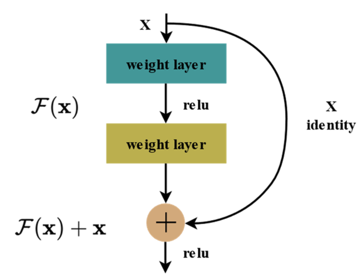
2.3. Network Structure of the Main Modules in MAFNet

The traditional image-classification algorithm has the problems of a single-feature scale, a low level of information richness, a poor classification effect, and a strong feature dependency, among others. The convolutional neural network, which has obvious advantages and is widely used to classify apple-leaf images, was selected to reduce the effect of the effectiveness and robustness of the artificially constructed features on the classification accuracy and to improve the classification accuracy [15,16,17,18]. The core idea of convolutional neural networks is using a local perceptual field, weight sharing, and pooling layers to simplify network parameters to provide the network with a certain degree of displacement, scale, scaling, and nonlinear deformation stability.

To solve the problem of network degradation, due to network redundancy and gradient disappearance, or explosion, caused by the deepening of network layers, the proposed model in this paper introduced the Res block [19] structure, shown in Figure 3, which can deepen the number of network layers while effectively reducing the effects of gradient disappearance and other problems, and which can enhance the connection between the feature maps generated by different convolutional layers to improve the recognition rate of the model. This structure can deepen the number of layers of the network while effectively reducing the effect of gradient disappearance and enhancing the connection between the feature maps generated by different convolutional layers, thus improving the recognition rate of the model. The following structure shows that x is the input of the residual block in this layer, and $F\left(x\right)$ is the output after linear change and activation in the first layer. Before the second layer is activated after the linear change, $F\left(x\right)$ is added to the input value x of the first layer, and then to the output after activation. The path of adding $x$ to the output value of the second layer before it is activated is called a “shortcut connection”. Through the shortcut connection, the upper-layer feature map $x$ is directly used as the initial result of the partial output, and the output is $H\left(x\right)=F\left(x\right)+x$, which becomes a constant map when $F\left(x\right)=0$. Therefore, such a structure is equivalent to learning the $H\left(x\right)-x$ part, which is the residual. Due to the presence of $x$, the presence of 1 in the backpropagation derivation always ensures that the gradient does not disappear or explode during the node-parameter update.

Due to the slight feature differentiation of the dataset provided in this paper, the high number of image background distractors, and the fact that simple convolution only operates in a local space, it is difficult to obtain enough information to capture the relationship between channels. Therefore, the SE block [20] module shown in Figure 4 is introduced, referring to the squeeze-and-excitation block, an attention-based feature map operation. The SE block first performs the squeeze operation on the feature map, i.e., the global average pooling operation in the channel dimension direction to compress $H\times W\times C$ to get $1\times 1\times C$ and obtain the global features in the channel dimension direction of the feature map. The expression of squeeze is shown in Equation (2):

$$z_c=F_{sq}\left(U_c\right)=\frac{1}{W\times H}{{\displaystyle \sum }}_{i=1}^W{{\displaystyle \sum }}_{j=1}^H{U}_c\left(i,j\right),z\in R^C,$$

(2)

where $U_c$ represents the feature map $U$ of the $c$th channel, $c\in C\left(1,2,\dots ,C\right)$; $H$ and $W$ represent the height and width, $i\in \left(1,2,\dots ,W\right)$, $j\in \left(1,2,\dots ,H\right)$. Then, the global features are subjected to the excitation operation to capture the relationship between channels. Here the gating mechanism in the form of the sigmoid function ($\sigma \left(x\right)$) is taken, and the excitation expression is shown in Equation (3):

$$s=F_{ex}\left(z,W\right)=\sigma \left(g\left(z,W\right)\right)=\sigma \left(W_{2}ReLU\left(W_{1}z\right)\right),$$

(3)

where $W_1\in R^{\frac{C}{r}\times C}$, $W_2\in R^{C\times \frac{C}{r}}$, $ReLU$ is the activation function, $ReLU=\left\{\begin{array}{c}x, x>0\\ 0, x\le 0\end{array}\right.$, $\sigma \left(x\right)=\frac{1}{1+e^{-x}}$. To reduce the complexity of the model as well as to enhance the generalization capability, this part is implemented using two fully connected layers, where the first fully connected layer achieves dimensionality reduction (the dimensionality reduction factor is $r$, which is a hyperparameter), followed by $ReLU$ activation, and then the original dimensionality is recovered by the second fully connected layer. Finally, the learned activation values of each channel are multiplied by the original features to achieve weight assignment over the channels and make the model more discriminative for channel features.

The feature extraction layer of the original ResNet model suffers from the problems of a large number of parameters and weak feature extraction ability, etc. The present model introduces the Contextual Transformer (CoT) block [21] structure to achieve the amplification of the feature distance between samples through the fusion modeling of the local static context and the dynamic global context. As shown in Figure 5, given an input feature $X$ of size $H\times W\times C$, three variables, $Q=X$, $K=X$, and $V=X{W}_v$, are defined. (Here, only $V$ is mapped to the feature, and the original $X$ values are still used for $Q$ and $K$.) A group convolution of $k\times k$ is performed on $K$ to obtain $K$ with local contextual information representation (denoted as $K^1$, $K^1\in R^{H\times W\times C}$), and this $K^1$ can be seen as static modeling on local information. Then Concat was performed on $K^1$ and $Q$. The result of Concat was subjected to two, consecutive $1\times 1$ convolution operations to obtain the attention matrix $A$. The expression is shown in Equation (4):

$$A=\left[K^1,Q\right]W_{\theta }{W}_{\delta }$$

(4)

Differing from the traditional self-attention, the $A$ matrix here is obtained by the interaction of the query information and the local context information $K^1$, not just the relationship between the query and the key. In other words, it is the self-attention mechanism enhanced through the guidance of local context modeling. Then, this attention map and $V$ are multiplied to obtain the dynamic context modeling $K^2$, and the expression is shown in Equation (5):

$$K^2=V\times A.$$

(5)

The final result is obtained after fusing $K^1$ of the local static context modeling, and $K^2$ of the global dynamic context modeling. Traditional self-attention can trigger feature interactions at different spatial locations very well. However, in the traditional self-attention mechanism, all query–key relations are used to compute the attention matrix via independent query–key pairs, and the rich context between keys is ignored, which dramatically limits visual representation learning. In contrast, the CoT block design, as shown in the figure below, unifies the context mining between adjacent keys and the self-attentive learning of 2D feature maps, using the contextual information between input keys to guide the self-attentive learning, thus avoiding the introduction of extra branches for context mining and improving the representational power of the network.

2.4. Network Structure Design of MAFNet

As shown in Figure 6, the network is composed of 1 $1\times 1$ convolution; in the middle are 4 convolutional modules with 3 convolutional structures in each module, where the convolutional modules are distributed in a symmetric design of [2,2,2,2], and finally, in a fully connected layer with a total of 26 convolutional modules.

After the image is input, the $1\times 1$ convolution operation is performed first. Then, the four convolutional modules are passed through the four convolutional modules. The 3 × 3 convolution is replaced by the CoT block in the original ResNet convolutional block. After the previous convolutional, excitation, and pooling operations, the extracted features are input into the fully connected layer, which plays the role of “classifier” in the convolutional neural network. The fully connected layer acts as a “classifier” in the convolutional neural network, which integrates the previous, highly abstracted features, maps the learned features to the sample space, uses the classifier Softmax function to calculate a probability for each classification case, and finally outputs the classification result. The expression of the Softmax function is shown in Equation (6):

$$\mathrm{Softmax}\left(z_j\right)=\frac{e^{z_j}}{{\sum }_{i=1}^n{e}^{z_i}},$$

(6)

where denotes the number of categories, $z_j$ denotes the output value of the $j$th node, $z_i$ denotes the output value of the $i$th node, and $e$ is a natural constant. In the experiment, the loss function is the cross-entropy, and the expression is shown in Equation (7):

$$L_{CE}=-{{\displaystyle \sum }}_{i=1}^N{l}_{i}log{p}_i,$$

(7)

where $l_i$ is the unique thermal encoding of tag $i$($i\in \left(0,\cdots ,N-1\right)$ and $N$ is the number of tags); if the target label is $i$ then $l_i=1$; all other labels are equal to 0; $p_i$ is the prediction probability of the $i$th label, that is, the value of Softmax.

Note that a too-small learning rate will lead to the slow convergence of the model, and a too-large learning rate may lead to the constant oscillation of the loss function during optimization and a failure to converge correctly. To make the model find the optimal parameters more quickly and accurately during training, a dynamic-learning-rate strategy is used to adjust the learning rate every 30 epochs, the expression of which is shown in Equation (8):

$$lr=l{r}_0\times {0.1}^{\frac{epoch}{30}},$$

(8)

where $lr$ is the current learning rate of the model, $l{r}_0$ is the initial learning rate, and $epoch$ is the total number of training rounds.

2.5. Configuration of the Experimental Environment

We conducted experiments on a computer with a CPU model Intel(R) Xeon(R) [email protected] (4 Cores), the details for which are shown in

Table 2. Software and hardware environment configuration.

Configuration Information
OS	Ubuntu 20.04.3 LTS
CPU	Intel(R)Xeon(R)[email protected] (4 Cores)
RAM	16 GB
GPU	NVIDIA GeForce GTX 1080
Video memory	8 GB
Code management software	PyCharm Community 2022.1.2
Language	Python 3.6.13
Deep-learning framework	PyTorch 1.2.0

.

3. Result

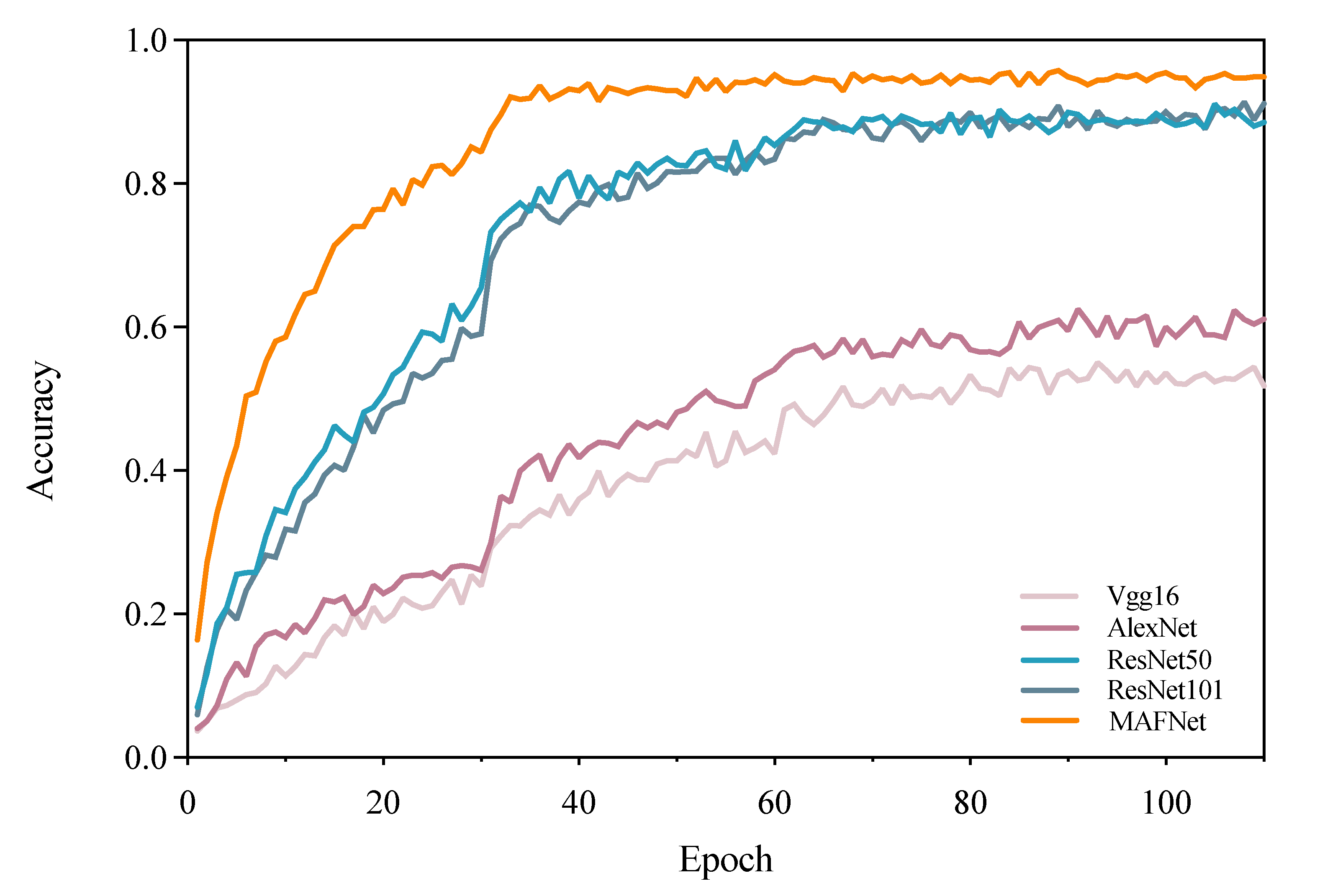
3.1. Performance Comparison of MAFNet with Other Models

In this paper, VGG16 [22], AlexNet [23], ResNet-50, and ResNet-101 were selected for comparison experiments, and it is apparent from Figure 7 that the model proposed in this paper exhibits a much higher level of accuracy than VGG16 or AlexNet on the apple-leaf dataset, and it has significantly improvements over native ResNet, with a more robust characterization capability. Since the experiment adopted a dynamic-learning-rate strategy, the accuracy of each model fluctuated to a certain extent after the 30th, 60th, and 90th rounds. It produced large accuracy fluctuations after reaching the 30th round of the change condition when the initial learning rate was significant. The step of the correction parameter decreased accordingly at a later stage due to the substantial reduction in the accuracy rate. Still, the overall trend was all on the rise, which proved the validity.

It is one-sided to evaluate the models only from the perspective of their accuracy; the size of the number of parameters is also an essential indicator of a model’s performance. Therefore, this study combined the parameter size of each model to evaluate the projection capability of the model comprehensively. From Figure 8, it is clear that the model proposed in this paper not only has a significant improvement in accuracy after replacing the convolution module of the feature extraction layer, but it also has a significant advantage over other models in terms of the number of parameters.

3.2. Performance Evaluation of MAFNet on Apple Leaf Dataset

Let us discuss the generalizability of MAFNet and its robustness.

The experiments were tested on 7200 test-set images. Figure 9 shows the two-dimensional line graphs of the accuracy and the loss values on the sample training set. The yellow curve in the figure shows that, as the number of iterations increases, the accuracy of the model increases dramatically in the first 30 rounds, showing a significant jump between 30 and 40 rounds, and the rising trend gradually flattens out after 40 rounds, the adjustment of the relevant weight parameters becomes smaller, the model starts to converge, and the accuracy of the final model on the training set is stable The absolute accuracy of the model on the training set is steady above 90%. The blue curve shows the loss value of the training set, and it can be seen that the loss value tends to decrease significantly in the first 30 rounds and then falls precipitously after the 30th round, after which the model gradually converges and approaches zero. Observing the two curves, the overall trend is towards the expected target, but there are minor fluctuations up and down, which indicates that the model can escape from the trap of the optimal local solution and shows apparent advantages in avoiding overfitting, and it can fully grasp the potential “universal law” in the leaf sample.

To reflect more visually the model’s ability to extract leaf features, the experiments were plotted using visualization tools to create a confusion matrix heatmap, as shown in Figure 10. In the heatmap, the vertical coordinates are the sample labels predicted by the model, and the horizontal coordinates are the actual sample labels. The main diagonal numbers are the number of sample images whose predicted values are the same as the true values, and the numbers in other positions are the number of sample images, predicted values of which are different from the true values. From Figure 5, it is evident that the main diagonal is dark, which indicates that the model has a good recognition effect on the leaf images from all 30 species. Among them, “Red General”, “SinanoGold”, and “Jonagold” had the best results, and all of the 240 test images were correctly predicted. The recognition effect of “Honglu”, “Huashuo”, “KCo8”, and “Shoufu 1” was relatively poor, with more than 10 bad scores. This was most likely due to the presence of more Fuji-line varieties among the selected species, which have more similar morphological traits in their leaves, which would increase the difficulty of classification in the model.

To further reflect the model’s performance, the accuracy, recall, and $F_{1\_score}$ of the model on each variety was calculated to evaluate the classification effectiveness of the model based on the data information in the confusion matrix. Based on the confusion matrix, we also needed to add the following metrics: $TP$, $FP$, $TN$, and $FN$ to define the specific parameters of classification accuracy for each species, which are true positive, false positive, true negative, and false negative, respectively. “Precision” refers to the proportion of positive cases correctly predicted by the model to the true positive cases, reflecting the check accuracy of the classifier, and the expression is shown in Equation (9):

$$Precision=\frac{TP}{TP+FP}$$

(9)

“Recall” refers to the proportion of positive cases correctly predicted by the model to the number of positive cases predicted by the model, reflecting the check-all rate of the classifier, and the expression is shown in Equation (10):

$$Recall=\frac{TP}{TP+FN}$$

(10)

$F_{1\_score}$ is the summed average of precision and recall, which is used to measure the comprehensive performance of the classifier, and the expression is shown in Equation (11):

$$F_{1\_score}=\frac{2\times Precision\times Recall}{Precision+Recall}$$

(11)

Since the classification of this experiment is a multiclassification problem, the average of the accuracy of each category needs to be calculated as the final metric. Therefore, macro-Precision ($\mathrm{macro}-P$), macro-Recall $\mathrm{macro}-R$), and macro-F1 were introduced to evaluate the “global” performance of the model, and the expressions are given by Equations (12)–(14) in turn:

$$\mathrm{macro}-P=\frac{1}{n}{{\displaystyle \sum }}_{i=1}^n{P}_i$$

(12)

$$\mathrm{macro}-R=\frac{1}{n}{{\displaystyle \sum }}_{i=1}^n{R}_i$$

(13)

$$\mathrm{macro}-F1=\frac{2\times \mathrm{macro}-P\times \mathrm{macro}-R}{\mathrm{macro}-P+\mathrm{macro}-R}$$

(14)

where $P_i$ refers to the precision rate $P$ of the $i$th label, and $R_i$ refers to the recall rate $R$ of the $i$th label.

When analyzing

Table 3. Accuracy for each cultivar.

Apple Cultivar	TP	FP	FN	TN	Precision	Recall	F1_score
Fuji 2001	238	2	17	6943	0.9917	0.9333	0.9616
Idared	236	4	4	6956	0.9833	0.9833	0.9833
Asta	235	5	3	6957	0.9792	0.9874	0.9833
Chengji No.1	237	3	12	6948	0.9875	0.9518	0.9693
Gala	239	1	3	6957	0.9958	0.9876	0.9917
GanHong	232	8	1	6959	0.9667	0.9957	0.9810
Ruby	239	1	1	6959	0.9958	0.9958	0.9958
Red General	240	0	8	6952	1.0000	0.9677	0.9836
Honglu	229	11	4	6956	0.9542	0.9828	0.9683
Golden Delicious	239	1	3	6957	0.9958	0.9876	0.9917
Huashuo	227	13	0	6960	0.9458	1.0000	0.9722
Jingning No.1	235	5	0	6960	0.9792	1.0000	0.9895
KCo8	227	13	6	6954	0.9458	0.9742	0.9598
Kuihua	232	8	1	6959	0.9667	0.9957	0.9810
Liuyuexian	238	2	4	6956	0.9917	0.9835	0.9876
Honey Crisp	231	9	0	6960	0.9625	1.0000	0.9809
Gala Mitchgla	234	6	7	6953	0.9750	0.9710	0.9730
Pinova	238	2	5	6955	0.9917	0.9794	0.9855
Ruixue	239	1	5	6955	0.9958	0.9795	0.9876
Ruiyang	238	2	2	6958	0.9917	0.9917	0.9917
Shoufu 1	226	14	3	6957	0.9417	0.9869	0.9638
Taiga	237	3	7	6953	0.9875	0.9713	0.9793
MATO	239	1	0	6960	0.9958	1.0000	0.9979
Orin	235	5	8	6952	0.9792	0.9671	0.9731
Rustless Goldspur	237	3	0	6960	0.9875	1.0000	0.9937
SinanoGold	240	0	0	6960	1.0000	1.0000	1.0000
Jonagold	240	0	0	6960	1.0000	1.0000	1.0000
Yanfu 0	232	8	7	6953	0.9667	0.9707	0.9687
Yanfu 3	238	2	18	6942	0.9917	0.9297	0.9597
Indo	239	1	5	6955	0.9958	0.9795	0.9876
macro-P = 0.9814		macro-R = 0.9818			macro-F1 = 0.9814

, if we analyze only from the accuracy perspective, “Shoufu 1” had the worst effect. The model had the worst detection rate for “Shoufu 1”. If we only look at the recall rate, “Fuji 2001” had the worst effect, that is, the worst detection rate for this variety, and a wide variety of types were mistaken as “Fuji 2001”, which confirms the view that the similarity between Fuji varieties is high. The evaluation of the model via the consideration of the values of these two aspects alone is not comprehensive enough, so we observed the $F_{1\_\mathrm{score}}$ and analyzed the precision and recall rates together, and we concluded that the best results were obtained for “SinanoGold” and “Jonagold”, while the worst result was “Yanfu 3” with 95.97%. Finally, we calculated 98.14% macro precision, 98.18% macro recall, and 98.14% $\mathrm{macro}-F1$, which further verified the model’s strong generalizability and robustness.

4. Conclusions

This paper establishes a deep-learning variety-classification model (MAFNet) based on the convolutional neural network according to the different growth stages of apple leaves. The distance of the features between the different types is expanded by improving and optimizing the ResNet network, incorporating multiple attention mechanisms. By comparing the networks of VGG16, AlexNet, ResNet-50, and ResNet-101 experimentally, the model has a more significant advantage in both the accuracy and the number of participants and achieves the effective recognition of 30 varieties of apples planted mainly in Northwest China under complex natural environments, which enriches the pool of currently available methods for apple-variety recognition. The final average accuracy of the model on the test set reached 98.14%, the number of parameters was only 72.81 MB, and the performance in terms of robustness and overfitting was also outstanding, which fully illustrates the excellent, comprehensive performance of the model and that it can effectively extract leaf features from images, proving the feasibility of using deep-learning networks for apple-variety recognition with significance for practical production and life.

Our future work is mainly based on the following considerations: (1) The number of varieties used in the experiment is far from sufficient when compared with the number in the market, and our group will push subsequent research to expand the number of apple varieties and collect more kinds of image data for the apple leaves. (2) Given that the model produces better results on apple-variety classification, we will consider its transplantation to the variety recognition of other types of fruit-tree leaves. (3) Other excellent neural network models, such as VoVNet [24], Swin Transformer [25], etc., will be studied to achieve the further optimization of this network model. (4) Since the traits characterized by organisms in different environments have certain differences, images of the same type of apple leaves in different regions will be added subsequently to enhance the generalizability of the model further. (5) We will further improve the identification mechanism and establish a deep-learning recognition model for the whole growth cycle of apples, from seed to leaf.

References

1. Brown, S. Apple; Fruit Breeding; Springer: Boston, MA, USA, 2012; pp. 329–367. [Google Scholar] [CrossRef]
2. Boyer, J.; Liu, R.H. Apple phytochemicals and their health benefits. Nutr. J. 2004, 3, 5–13. [Google Scholar] [CrossRef] [PubMed]
3. Cong, P. Apple Varieties in China; China Agriculture Press: Beijing, China, 2015; pp. 2–3. [Google Scholar]
4. Luo, W.; Huan, S.; Fu, H.; Wen, G.; Cheng, H.; Zhou, J.; Wu, H.; Shen, G.; Yu, R. Preliminary study on the application of near infrared spectroscopy and pattern recognition methods to classify different types of apple samples. Food Chem. 2011, 128, 555–561. [Google Scholar] [CrossRef] [PubMed]
5. Wu, X.; Wu, B.; Sun, J.; Li, M.; Du, H. Discrimination of Apples Using Near Infrared Spectroscopy and Sorting Discriminant Analysis. Int. J. Food Prop. 2016, 19, 1016–1028. [Google Scholar] [CrossRef]
6. Ma, H.; Wang, R.; Cai, C.; Wang, D. Rapid Identification of Apple Varieties Based on Hyperspectral Imaging. Trans. Chin. Soc. Agric. Mach. 2017, 48, 305–312. [Google Scholar]
7. Ni, J.; Yang, H.; Li, J.; Han, Z. Variety identification of peanut pod based on improved AlexNet. J. Peanut Sci. 2021, 50, 14–22. [Google Scholar] [CrossRef]
8. Park, J.; Kim, D.; Kim, J.; Kim, H. CNN based modeling and classification for variety of apples. J. D-Cult. Arch. 2021, 4, 63–70. [Google Scholar]
9. Geng, L.; Huang, Y.; Guo, Y. Apple Variety Classification Method Based on Fusion Attention Mechanism. Trans. Chin. Soc. Agric. Mach. 2022, 1–11. [Google Scholar]
10. Al-Shawwa, M.O.; Abu-Naser, S.S. Classification of apple fruits by deep learning. Int. J. Acad. Eng. Res. (IJAER) 2020, 3, 1–6. [Google Scholar]
11. Jeong, S.; Yoe, H. Fruit classification system using deep learning. J. Knowl. Inf. Technol. Syst. 2018, 13, 589–595. [Google Scholar]
12. Grinblat, G.L.; Uzal, L.C.; Larese, M.G.; Granitto, P.M. Deep learning for plant identification using vein morphological patterns. Comput. Electron. Agric. 2016, 127, 418–424. [Google Scholar] [CrossRef]
13. Baldi, A.; Pandolfi, C.; Mancuso, S.; Lenzi, A. A leaf-based back propagation neural network for oleander (Nerium oleander L.) cultivar identification. Comput. Electron. Agric. 2017, 142, 515–520. [Google Scholar] [CrossRef]
14. Liu, C.; Han, J.; Chen, B.; Mao, J.; Xue, Z.; Li, S. A Novel Identification Method for Apple (Malus domestica Borkh.) Cultivars Based on a Deep Convolutional Neural Network with Leaf Image Input. Symmetry 2020, 12, 217. [Google Scholar] [CrossRef]
15. Zhao, K.; Liu, X.; Ji, J. Automatic body condition scoring method for dairy cows based on EfficientNet and convex hull feature of point cloud. Trans. Chin. Soc. Agric. Mach. 2021, 52, 192–201. [Google Scholar]
16. Zhu, Y.; Xia, J.; Zeng, R.; Zheng, K.; Du, J.; Liu, Z. Prediction model of rotary tillage power consumption in paddy stubble field based on discrete element method. Trans. Chin. Soc. Agric. Mach. 2020, 51, 42–50. [Google Scholar]
17. Sun, J.; Chen, H.; Wang, Z.; Ou, Z.; Yang, Z.; Liu, Z.; Duan, J. Study on plowing performance of EDEM low-resistance animal bionic device based on red soil. Soil Tillage Res. 2020, 196, 104336. [Google Scholar] [CrossRef]
18. Hu, H.; Li, H.; Li, C.; Wang, Q.; He, J.; Li, W.; Zhang, X. Design and experiment of broad width and precision minimal tillage wheat planter in rice stubble field. Trans. Chin. Soc. Agric. Eng. 2016, 32, 24–32. [Google Scholar]
19. He, K.; Zhang, X.; Ren, S.; Sun, J. Deep residual learning for image recognition. In Proceedings of the IEEE Conference on Computer Vision and Pattern Recognition, Las Vegas, NV, USA, 26 June–1 July 2016; pp. 770–778. [Google Scholar]
20. Hu, J.; Shen, L.; Sun, G. Squeeze-and-excitation networks. In Proceedings of the IEEE Conference on Computer Vision and Pattern Recognition, Salt Lake City, UT, USA, 18–22 June 2018; pp. 7132–7141. [Google Scholar]
21. Li, Y.; Yao, T.; Pan, Y.; Mei, T. Contextual transformer networks for visual recognition. IEEE Trans. Pattern Anal. Mach. Intell. 2022, 1. [Google Scholar] [CrossRef] [PubMed]
22. Simonyan, K.; Zisserman, A. Very deep convolutional networks for large-scale image recognition. arXiv 2014, arXiv:1409.1556. [Google Scholar]
23. Krizhevsky, A.; Sutskever, I.; Hinton, G.E. Imagenet classification with deep convolutional neural networks. In Proceedings of the Advances in Neural Information Processing Systems, Lake Tahoe, NV, USA, 3–8 December 2012; Volume 25. [Google Scholar]
24. Lee, Y.; Hwang, J.W.; Lee, S.; Bae, Y.; Park, J. An energy and GPU-computation efficient backbone network for real-time object detection. In Proceedings of the IEEE/CVF Conference on Computer Vision and Pattern Recognition Workshops, Long Beach, CA, USA, 16–17 June 2019. [Google Scholar]
25. Liu, Z.; Lin, Y.; Cao, Y.; Hu, H.; Wei, Y.; Zhang, Z.; Lin, S.; Guo, B. Swin transformer: Hierarchical vision transformer using shifted windows. In Proceedings of the IEEE/CVF International Conference on Computer Vision, Montreal, QC, Canada, 11–17 October 2021; pp. 10012–10022. [Google Scholar]
Figure 1. Comparison images from before and after data augmentation.
Symmetry 14 01671 g001
Figure 2. Distribution of color skew values of images after data augmentation.
Symmetry 14 01671 g002
Figure 3. Framework of Res block. Note: The weight layer is the convolution operation layer, and ReLU is the activation function.
Symmetry 14 01671 g003
Figure 4. Squeeze-and-excitation block. Note: In the figure, W, H, and C indicate the width, height, and the number of channels of the input and output values, respectively. The Scale indicates multiplying the learned activation value of each channel by the original feature value.
Symmetry 14 01671 g004
Figure 5. Contextual Transformer block.
Symmetry 14 01671 g005
Figure 6. Network structure of MAFNet. Note: W, H, and Channel denote the width, height, and the number of channels of input and output values, respectively; Conv denotes convolution operation; Average Pooling is the average pooling operation; Fully Connected is the fully connected operation; SoftMax is the probabilistic output function.
Symmetry 14 01671 g006
Figure 7. Accuracy comparison of deep-learning networks on the apple-leaf dataset. Note: The vertical coordinate indicates the accuracy rate, and the horizontal coordinate indicates the number of training rounds.
Symmetry 14 01671 g007
Figure 8. Comparison of the number of parameters. Note: The vertical coordinate indicates the number of parameters, and the horizontal coordinate indicates the model’s name.
Symmetry 14 01671 g008
Figure 9. Accuracy and Loss. Note: The left vertical coordinate indicates the accuracy rate, the right vertical coordinate indicates the loss value, and the horizontal coordinate indicates the number of training rounds.
Symmetry 14 01671 g009
Figure 10. Confusion matrix thermodynamic diagram of the test set. Note: The number represents the number of corresponding labels predicted by the model, and the value ranges from 0–240; the higher the number, the darker the color.
Symmetry 14 01671 g010