
The Attack-Block-Court Defense Algorithm: A New Volleyball Index Supported by Data Science

 , , and
Abstract
:1. Introduction
2. Methodology
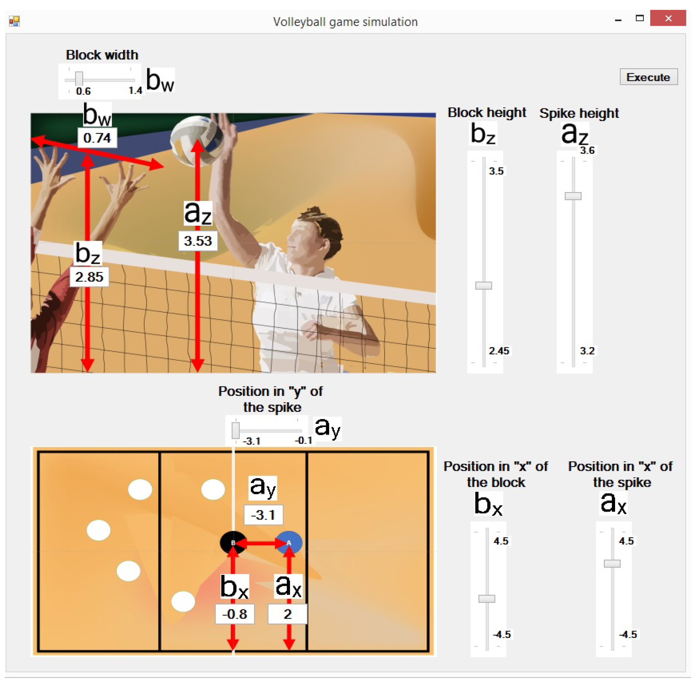
2.1. Physical Model
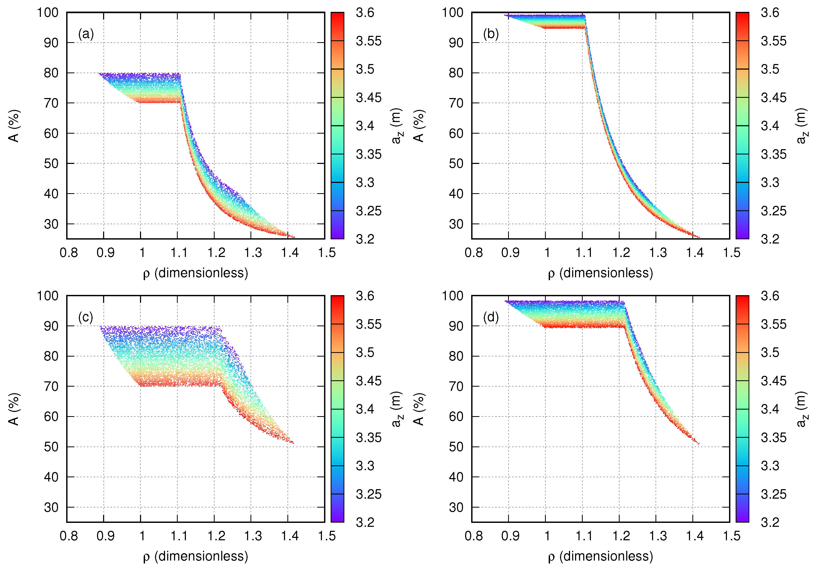
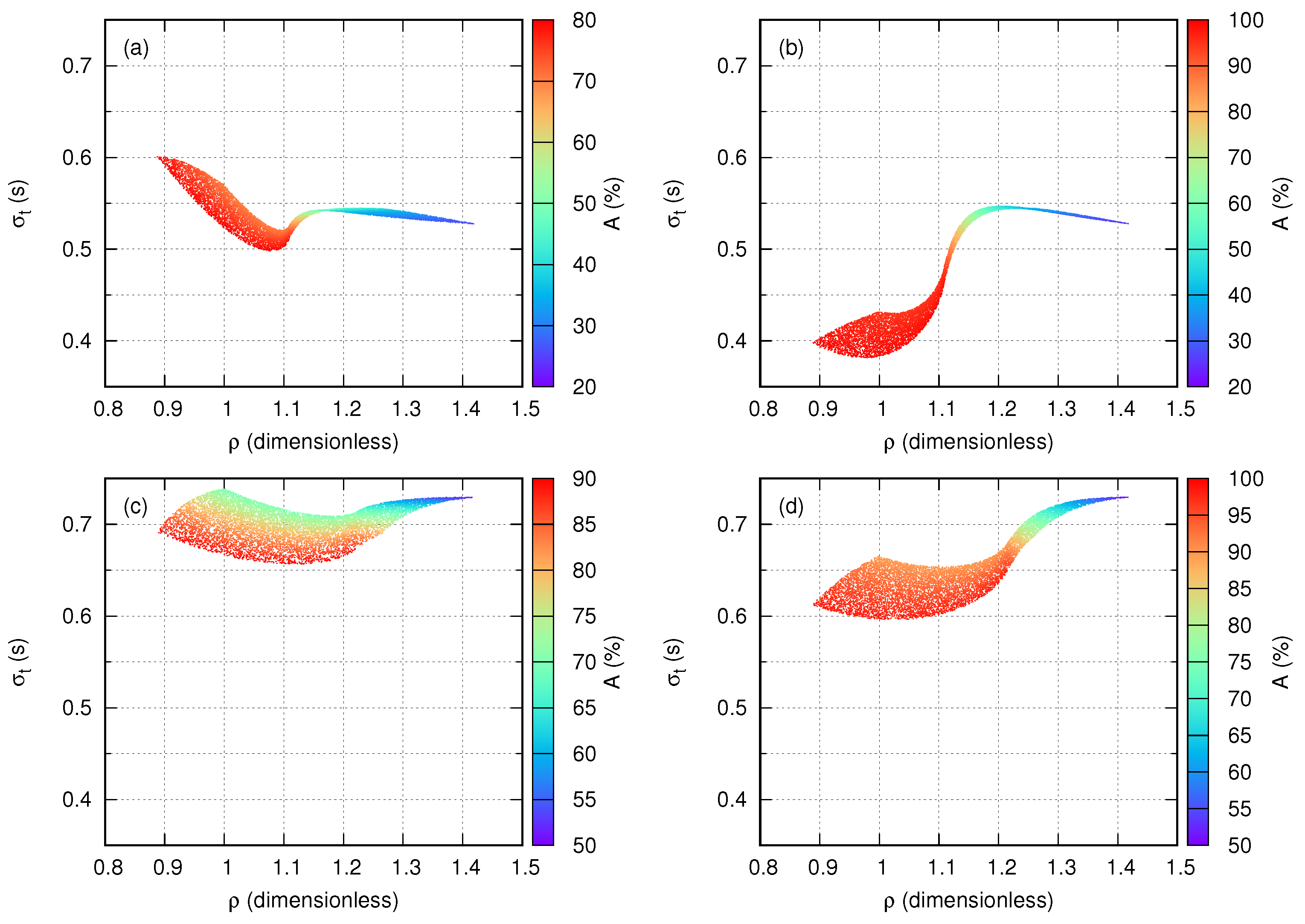
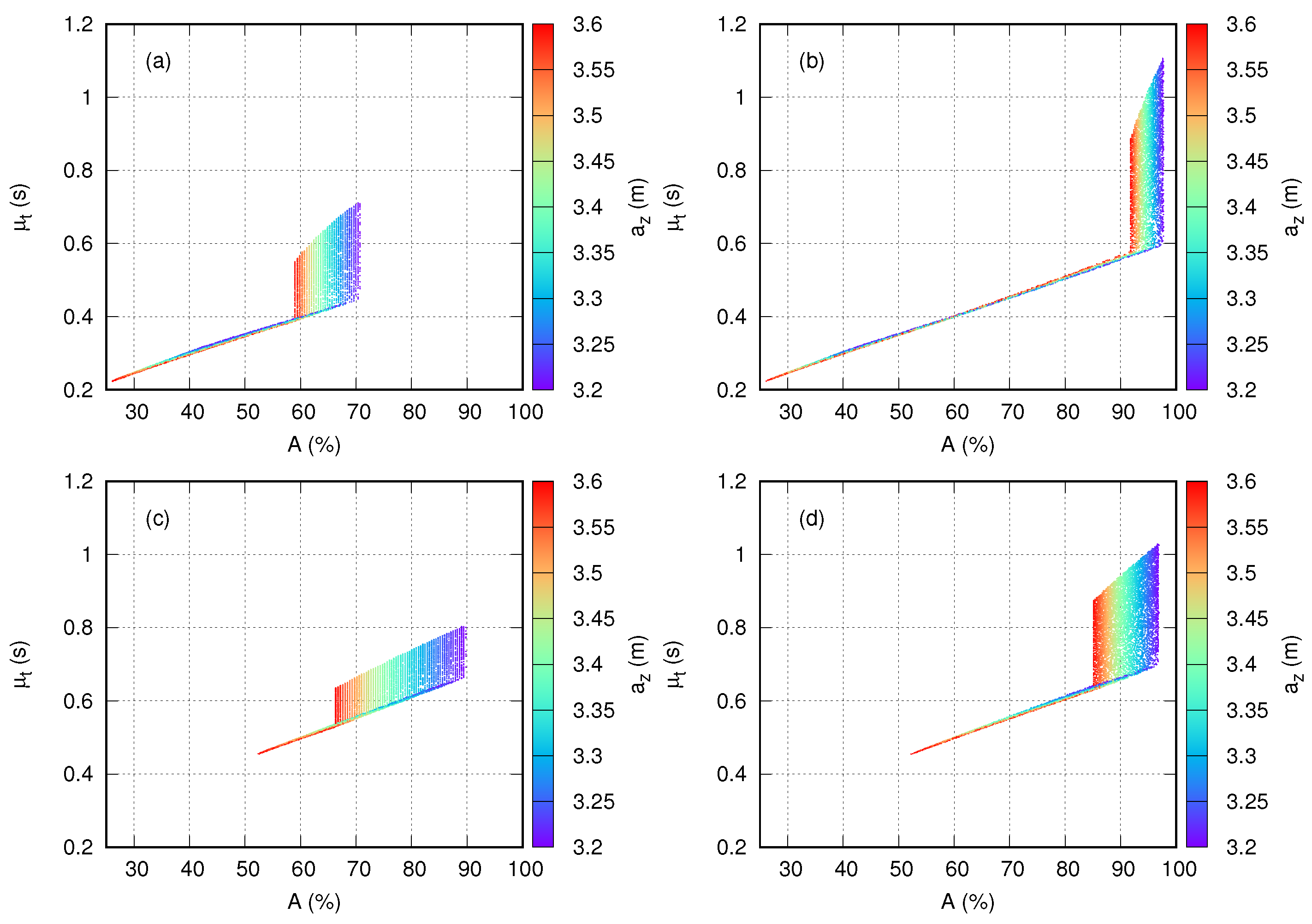
2.2. Covered Area and Impact Time
- from a to s; taking a as the initial point and s as the final point,
- from s to ; taking s as the initial point and as the final point.
2.3. The Attack-Block-Court Defense Algorithm (The ABCD Algorithm)
| Algorithm 1 Pseudo-code of the ABCD algorithm for one simulation. |
|
- Input data: 3D positions of the attacker and blocker(s);
- Consider one cell of the court;
- Consider blocker 1;
- Calculate the ball’s trajectory of the worst scenario;
- If it applies, repeat Step 4 for blockers 2 and 3;
- Repeat Steps 3–5 for the rest of the cells;
- Calculate the output data.
3. Results
4. Discussion
4.1. Application in Matches and Training
4.2. Limitations of the Model
- It can consider the five categories of block opposition. Here, we presented three of them: single blocking, broken double blocking, and triple blocking.
- Block position and attack zone are our input data in the way of the 3D locations of such players.
- It considers two of the five times of an attack: the ball hit and the block time.
- It proposes three additional variables (covered area, average impact time and its standard deviation) that have not been considered inside their wide set of variables.
5. Conclusions
- To add more variables and randomness to the block’s model with the aim of representing complex scenarios that are not discussed in this work, such as small modifications in the ball’s trajectory caused by a light contact of the blocker’s fingers.
- To illustrate representative cases of double and triple block.
- To adapt the methodology to the serve, but including drag and Magnus forces to the ball’s equations of motion.
- To consider more statistical data in the algorithm, such as trends in the direction of the spike, and the percentage of the effectiveness of each player.
Author Contributions
Funding
Institutional Review Board Statement
Informed Consent Statement
Data Availability Statement
Acknowledgments
Conflicts of Interest
Appendix A


References
- Fister, I.; Ljubič, K.; Suganthan, P.N.; Perc, M.; Fister, I. Computational intelligence in sports: Challenges and opportunities within a new research domain. Appl. Math. Comput. 2015, 262, 178–186. [Google Scholar] [CrossRef]
- Sarlis, V.; Chatziilias, V.; Tjortjis, C.; Mandalidis, D. A Data Science approach analysing the Impact of Injuries on Basketball Player and Team Performance. Inf. Syst. 2021, 99, 101750. [Google Scholar] [CrossRef]
- Grossi, V.; Giannotti, F.; Pedreschi, D.; Manghi, P.; Pagano, P.; Assante, M. Data science: A game changer for science and innovation. Int. J. Data Sci. Anal. 2021, 11, 263–278. [Google Scholar] [CrossRef]
- Aguirre-López, M.A.; Morales-Castillo, J.; Díaz-Hernández, O.; Escalera Santos, G.J.; Almaguer, F.J. Trajectories reconstruction of spinning baseball pitches by three-point-based algorithm. Appl. Math. Comput. 2018, 319, 2–12. [Google Scholar] [CrossRef]
- Aguirre-López, M.A.; Díaz-Hernández, O.; Hueyotl-Zahuantitla, F.; Morales-Castillo, J.; Almaguer, F.J.; Escalera Santos, G.J. A cardioid-parametric model for the Magnus effect in baseballs. Appl. Math. Comput. 2019, 45, 2097–2109. [Google Scholar] [CrossRef]
- Nathan, A.M. The effect of spin on the flight of a baseball. Am. J. Phys. 2008, 76, 119–124. [Google Scholar] [CrossRef] [Green Version]
- Nathan, A.M.; Crisco, J.J.; Greenwald, R.M.; Russell, D.A.; Smith, L.V. A comparative study of baseball bat performance. Sport. Eng. 2011, 13, 153. [Google Scholar] [CrossRef]
- Van Haaren, J.; Ben Shitrit, H.; Davis, J.; Fua, P. Analyzing Volleyball Match Data from the 2014 World Championships Using Machine Learning Techniques. In Proceedings of the 22nd ACM SIGKDD International Conference on Knowledge Discovery and Data Mining, San Francisco, CA, USA, 13–17 August 2016; KDD ’16. Association for Computing Machinery: New York, NY, USA, 2016; pp. 627–634. [Google Scholar] [CrossRef] [Green Version]
- Song, W.; Xu, M.; Dolma, Y. Design and Implementation of Beach Sports Big Data Analysis System Based on Computer Technology. J. Coast. Res. 2019, 94, 327–331. [Google Scholar] [CrossRef]
- Loffing, F.; Stern, R.; Hagemann, N. Pattern-induced expectation bias in visual anticipation of action outcomes. Acta Psychol. 2015, 161, 45–53. [Google Scholar] [CrossRef]
- Srl, G.S.I. Data Volley 4. 2022. Available online: https://www.dataproject.com/ (accessed on 14 May 2022).
- Srl, D.P.S.S. Data Volley Media, 2007th ed.; Data Project Sport Software Srl; Head Office & Marketing Department: Bologna, Italy, 2012; p. 66. [Google Scholar]
- Harabagiu, N. The Importance of Using the “Data Volley” Software and of the “Data Video” System in the Tactical Training of the Middle Blocker for Official Games. Gymnasium 2020, XXI, 34–41. [Google Scholar] [CrossRef]
- Silva, M.; Lacerda, D.; João, P.V. Game-Related Volleyball Skills that Influence Victory. J. Hum. Kinet. 2014, 41, 173–179. [Google Scholar] [CrossRef] [PubMed] [Green Version]
- Giatsis, G.; Martinez, A.L.; García, G.M. The efficacy of the attack and block in game phases on male FIVB and CEV beach volleyball. J. Hum. Sport Exerc. 2015, 10, 537–549. [Google Scholar] [CrossRef] [Green Version]
- Queiroga, M.; Matias, C.; Greco, P.; Graca, A.; Mesquita, I. The dimension of the high-level setter’s tactical strategic knowledge: Study with setters of Brazilian national. Braz. J. Phys. Educ. 2005, 111–119. [Google Scholar]
- Palao, J.M.; Santos, J.A.; Urena, A. Effect of reception and dig efficacy on spike performance and manner of execution in volleyball. J. Hum. Mov. Stud. 2006, 51, 221–238. [Google Scholar]
- Liskevych, T. Volleyball Defense Systems and Strategies. 2021. Available online: https://www.theartofcoachingvolleyball.com/defensive-systems/ (accessed on 8 May 2022).
- Liskevych, T. Dominating Defensive Systems. In The Volleyball Coaching Bible; Shondell, D., Reynaud, C., Eds.; Human Kinetics Publishers, Inc.: Champaign, IL, USA, 2002. [Google Scholar]
- Marcelino, R.; Mesquita, I.; Sampaio, J.; Morae, J.C. Estudo dos indicadores de rendimento em voleibol em função do resultado do set. Rev. Bras. Educ. FíSica Esporte 2010, 24, 69–78. [Google Scholar] [CrossRef] [Green Version]
- Costa, G.; Afonso, J.; Brant, E.; Mesquita, I. Differences in game patterns between male and female youth volleyball. Kinesiology 2012, 44, 60–66. Available online: https://hrcak.srce.hr/en/file/124413 (accessed on 26 June 2022).
- Drikos, S.; Sotiropoulos, K.; Barzouka, K.; Angelonidis, Y. The contribution of skills in the interpretation of a volleyball set result with minimum score difference across genders. Int. J. Sport. Sci. Coach. 2020, 15, 542–551. [Google Scholar] [CrossRef]
- Afonso, J.; Mesquita, I. Determinants of block cohesiveness and attack efficacy in high-level women’s volleyball. Eur. J. Sport Sci. 2011, 11, 69–75. [Google Scholar] [CrossRef]
- Araújo, R.M.; Castro, J.; Marcelino, R.; Mesquita, I.R. Relationship between the Opponent Block and the Hitter in Elite Male Volleyball. J. Quant. Anal. Sport. 2010, 6, 4. [Google Scholar] [CrossRef]
- Marelić, N.; Rešetar, T.; Janković, V. Discriminant analysis of the sets won and the sets lost by one team in a1 italian volleyball league—A case study. Kinesiology 2004, 36, 75–82. [Google Scholar]
- Palao, J.M.; Santos, J.A.; Ureña, A. Effect of team level on skill performance in volleyball. Int. J. Perform. Anal. Sport 2004, 4, 50–60. [Google Scholar] [CrossRef]
- Hernández-Hernández, E.; Montalvo-Espinosa, A.; García-de Alcaraz, A. A Time-Motion Analysis of the Cross-Over Step Block Technique in Volleyball: Non-Linear and Asymmetric Performances. Symmetry 2020, 12, 1027. [Google Scholar] [CrossRef]
- Xu, W. Teaching And Training Methods Of Volleyball Blocking Technique. Int. J. Front. Sociol. 2020, 2, 60–67. [Google Scholar] [CrossRef]
- Piras, A.; Lobietti, R.; Squatrito, S. A study of saccadic eye movement dynamics in volleyball: Comparison between athletes and non-athletes. J. Sport. Med. Phys. Fit. 2010, 50, 99–108. [Google Scholar]
- Piras, A.; Lobietti, R.; Squatrito, S. Response Time, Visual Search Strategy, and Anticipatory Skills in Volleyball Players. J. Ophthalmol. 2014, 2014, 189268. [Google Scholar] [CrossRef]
- Berriel, G.P.; Schons, P.; Costa, R.R.; Oses, V.H.S.; Fischer, G.; Pantoja, P.D.; Kruel, L.F.M.; Peyré-Tartaruga, L.A. Correlations Between Jump Performance in Block and Attack and the Performance in Official Games, Squat Jumps, and Countermovement Jumps of Professional Volleyball Players. J. Strength Cond. Res. 2021, 35, S64–S69. [Google Scholar] [CrossRef] [PubMed]
- Ficklin, T.; Lund, R.; Schipper, M. A comparison of jump height, takeoff velocities, and blocking coverage in the swing and traditional volleyball blocking techniques. J. Sport. Sci. Med. 2014, 13, 78–83. [Google Scholar]
- Epic-Sports. Volleyball Glossary. 2022. Available online: https://volleyball.epicsports.com/volleyball-glossary.html (accessed on 1 February 2022).
- Hibbeler, R.C. Kinematics of a Particle. In Engineering Mechanics. Dynamics, 14th ed.; Pearson Prentice Hall: Hoboken, NJ, USA, 2015. [Google Scholar]
- Official Volleyball Rules 2021–2024. Approved by the 37th FIVB World Congress 2021. Available online: https://www.tvf.org.tr/_dosyalar/MHGK_Belgeler/FIVB-Volleyball_Rules_2021_2024-EN.pdf (accessed on 1 February 2022).
- R Core Team. R: A Language and Environment for Statistical Computing; R Foundation for Statistical Computing: Vienna, Austria, 2013. [Google Scholar]
- Williams, T.; Kelley, C.; Merritt, E.A.; Bersch, C.; Bröker, H.-B.; Campbell, J.; Cunningham, R.; Denholm, D.; Elber, E.; Fearick, R. Gnuplot 5.4: An Interactive Plotting Program. 2021. Available online: http://www.gnuplot.info (accessed on 15 May 2022).
- Sharp, J. Microsoft Visual C# Step by Step, 9th ed.; Microsoft Press: Washington, DC, USA, 2018; p. 832. [Google Scholar]
- Laporta, L.; Medeiros, A.I.A.; Vargas, N.; de Oliveira Castro, H.; Bessa, C.; João, P.V.; Costa, G.D.C.T.; Afonso, J. Coexistence of Distinct Performance Models in High-Level Women’s Volleyball. J. Hum. Kinet. 2021, 78, 161–173. [Google Scholar] [CrossRef]
- Laporta, L.; Nikolaidis, P.; Thomas, L.; Afonso, J. Attack Coverage in High-Level Men’s Volleyball: Organization on the Edge of Chaos? J. Hum. Kinet. 2015, 47, 249–257. [Google Scholar] [CrossRef] [Green Version]


Publisher’s Note: MDPI stays neutral with regard to jurisdictional claims in published maps and institutional affiliations. |
© 2022 by the authors. Licensee MDPI, Basel, Switzerland. This article is an open access article distributed under the terms and conditions of the Creative Commons Attribution (CC BY) license (https://creativecommons.org/licenses/by/4.0/).
Share and Cite
Cantú-González, J.R.; Hueyotl-Zahuantitla, F.; Castorena-Peña, J.A.; Aguirre-López, M.A. The Attack-Block-Court Defense Algorithm: A New Volleyball Index Supported by Data Science. Symmetry 2022, 14, 1499. https://doi.org/10.3390/sym14081499
Cantú-González JR, Hueyotl-Zahuantitla F, Castorena-Peña JA, Aguirre-López MA. The Attack-Block-Court Defense Algorithm: A New Volleyball Index Supported by Data Science. Symmetry. 2022; 14(8):1499. https://doi.org/10.3390/sym14081499
Chicago/Turabian StyleCantú-González, José Roberto, Filiberto Hueyotl-Zahuantitla, Jesús Abraham Castorena-Peña, and Mario A. Aguirre-López. 2022. "The Attack-Block-Court Defense Algorithm: A New Volleyball Index Supported by Data Science" Symmetry 14, no. 8: 1499. https://doi.org/10.3390/sym14081499