
Mapping Natural Orbits around Io
by
 , , and
Thamis C. F. Carvalho Ferreira
1,* ,
,
Antonio F. Bertachini A. Prado
2,3,
Silvia M. Giuliatti Winter
1 and
Lucas S. Ferreira
1 1
Grupo de Dinâmica Orbital e Planetologia (GDOP), São Paulo State University (UNESP), São Paulo 12516-410, Brazil
2
Academy of Engineering, Peoples’ Friendship University of Russia (RUDN University), 6 Miklukho-Maklaya Street, 117198 Moscow, Russia
3
Postgraduate Division, National Institute for Space Research (INPE), São José dos Campos 12227-010, Brazil
*
Author to whom correspondence should be addressed.
Symmetry 2022, 14(7), 1478; https://doi.org/10.3390/sym14071478
Submission received: 31 May 2022
/
Revised: 7 July 2022
/
Accepted: 13 July 2022
/
Published: 19 July 2022
(This article belongs to the Special Issue Advances in Mechanics and Control)
Abstract
:As the most volcanically active celestial body in the Solar System, Io is a natural satellite of Jupiter due to its proximity to the planet and the fact that it is in mean motion resonance, known as the Laplace resonance, with the natural satellites Europa and Ganymede. This natural satellite is a good candidate to be visited by future missions. In this sense, the present work has the goal of studying and mapping the best initial orbital conditions for orbits around Io, considering the symmetrical or asymmetical perturbative effects of a third body (Jupiter) and the term from the mass configuration of Io. The initial orbital parameters of the probe were investigated through a set of numerical simulations. The results showed that although most orbits around Io have lifetimes of less than 6 months, some regions were found where the initial conditions of the orbits provided satisfactory times for the accomplishment of future missions around Io.
1. Introduction
Over the last few decades, since the first space launches, astronomical research has been improving. As a result of these advances, we have the possibility of studying planets, natural satellites, and other bodies in the Solar System using space probes. Exploration missions to the Moon began in 1959 with the launch of Luna 1, which was the first space vehicle to fly by on the Moon. Subsequently, several exploration missions were carried out, and important discoveries were made about several planets and natural satellites of the Solar System. Among these studies, ref. [1] analyzed data from Mariner 4, Mars 3, 4, and 5, which detected and measured the range of the magnetic moment of Mars. The Mariner 5 mission performed observations that helped study the magnetic field and atmospheric composition of Venus [2]. Voyager 1, Voyager 2, and Galileo probes have gathered important data about the moons of Jupiter, as well as the Cassini–Huygens mission, which carried out studies in Saturn and its satellite and ring system [3]. By analyzing the data brought back by Voyager 1, volcanic activity was detected on Io [4]. Details of the surface of Europa suggested recent geological activity [5], and evidence of an underground ocean [6] was brought back by both missions, Voyager˜2 and Galileo. The Cassini mission detected plumes of water vapor ejected from the south pole of Enceladus and also found evidence of liquid water [7]. All these results have motivated the scientific community to plan missions to map, measure and sample various moons and asteroids of the Solar System ([8,9,10]). Within this scenario of planning future missions to explore and study natural satellites present in the Solar System, Io also presents itself as a good candidate to be visited in future missions. Due to its proximity to the planet and the fact that it is in mean motion resonance, known as the Laplace resonance, with the natural satellites Europa and Ganymede, Io has a high tidal energy dissipation, resulting in the melting of a large fraction of its mass. Therefore, this moon is the most active body and with the most active volcano of the Solar System [11]. This is one of the many interests of the scientific community in the study of Io. Thus, the objective of this work is to build maps of natural orbits around the natural satellite Io, considering the effects of the gravitational perturbations from Jupiter and the flattening of Io.
It is known that sending probes to study celestial bodies requires detailed planning. Prior knowledge of some characteristics or information about the body and the environment that surrounds it are important. In the case of natural satellites, the disturbance coming from the planets in the regions where these bodies are studied is an essential factor to be considered in the search for orbits to insert the probes. Previous works, such as [12,13,14,15], were some of the pioneers in the investigation of third-body perturbations, more precisely lunisolar perturbations. Taking into account the previous works considering three-body problem solving, ref. [16] proposes the application of third-body perturbation theory to study and determine the lifetimes of orbits around natural satellites of the Solar System. Researchers verified the temporal evolution of the orbital elements of the probe by comparing three models: a double-average model considering the perturbing function expanded to the second order, the same model expanded to the fourth order, and the complete numerical integration of the circular restricted three-body problem using the 8th order Runge–Kutta method. Later, researchers presented lifetime maps for natural satellites through numerical integration of the problem, considering Io as one of the moons under study.
A comparison between the restricted three-body elliptical full model and the single and double averaged models was made in [17]. After that, ref. [18] used the solution obtained by [19] for the three-body elliptical problem and obtained the lifetime for the Earth–Moon system as a function of the initial eccentricities and inclinations of the probe. In [20], lifetime maps were obtained for the Callisto–Jupiter system assuming different values for the eccentricity of the perturbing body, also taking into account the and the order 2 of the sectoral flattening coefficient, , of Callisto. A study on the lifetime of orbits of a probe around Europa, considering the gravitational effects of Jupiter and the terms and of Europa, using a perturbative potential expanded in a series of Legendre polynomials and the double average method, was presented by [21]. This work presents contributions in the study of the lifetime of orbits with high inclinations, the effects due to and critical inclinations. In order to increase the times of some orbits, ref. [21] also presents studies performing corrective maneuvers in certain orbital conditions.
In this sense, ref. [22] studied the motion of an artificial satellite around Europa, taking into account the disturbance from Jupiter and the effects of the non-sphericity of Europa. The paper analyzed quasi-polar and low-altitude orbits using the double-average and single-average methods. Unstable frozen orbits lasting approximately 200 days were found. In [23], considering studies around Europa, a comparison between the simple average model and the numerical solution was presented. However, the orbit of the disturbing body was considered to be circular. Several frozen orbits, with low altitudes and inclinations, with long lifetimes were obtained. In [24,25], searches were made for orbits around Europa with longer lifetimes. Their studies found polar orbits with long lifetimes and near-circular frozen orbits with smaller amplitudes of variations of the orbital elements.
The work developed by [26] considered the problem of critical and quasi-critical inclinations for orbits of artificial satellites around the Moon. Taking into account the terms and of the gravitational potential and the rotation of the Moon, they present the dynamics of the system using a Hamiltonian function. Different combinations were considered for the perturbations included in the model. The analysis of the results showed that the values of the three parameters, , and the Moon rotation, affected the amplitude of the pericenter libration and the value of the quasi-critical inclinations. They also described how the rotation of the Moon was responsible for smoothing certain effects in the system. Using the same approach of orbits with critical inclinations, ref. [27] analyzed the the effects of the sectoral term in dynamics that already presented the perturbations of the flattening of a natural satellite. Considering a Hamiltonian approach, the authors applied a nonlinear optimization method to determine critical and quasi-critical orbits. His study focused on the natural satellite Io considering direct and retrograde orbits.
Considering the growing interest in the study of Io, as shown by the works of [28,29,30], the volcanism of Io was studied in detail by [31], where Voyager and Galileo data were used to produce the first global geological map. Improving and obtaining new maps was also one of the topics covered in this work. One of the most important factors highlighted was the acquisition of new data that can be used in future missions. In view of the importance of studying this moon, flybys for Ganymede, Europa, and Io [32] are planned for 2024, according to the Juno mission extension schedule, which has as one of its objectives the investigation of several aspects that will be important for future exploration missions. In this sense, the present work aims to bring contributions for future missions through the study of orbits around Io.
Another important point to be mentioned is that Io is in a region with high radiation levels. For this reason, only flyby missions were made up to now. However, there are advances in shielding techniques to make missions to Io possible. Therefore, orbits with longer duration will be required and deserve to be studied, which is the main goal of the present paper.
2. Materials and Methods
In our work, the scenario of interest is composed by three bodies: Io, a space probe, and Jupiter. We configured the system to consider that the origin of the reference system is centered in Io, in which Jupiter describes a circular and coplanar orbit. The probe is in three-dimensional orbit internal to Jupiter, where , , , and correspond, respectively, to the semi-major axis, inclination, argument of pericentre, and longitude of the ascending node of the orbit of the probe around Io. Considering that the goal of our study is to investigate the lifetime of natural orbits around Io, we consider the perturbative effects due to Jupiter and the asymmetry of the mass configuration, the non-sphericity of Io, represented by the zonal second harmonic . Thus, according to [16,33], the equations of motion for the proposed system can be expressed in the form:
where
where , and are the mass ratios of the probe, Io and Jupiter, respectively, and and are the position vectors of the probe and Jupiter, relative to Io. In Equations (2)–(4), which correspond to the components of the acceleration due to the flattening of Io, R is the equatorial radius of the natural satellite and is the second harmonic zonal term.
To obtain the time evolution of the osculating orbital elements of the probe, we implement the restricted circular three-body problem plus the terms referring to the non-sphericity of Io, based on Equation (1). We used a numerical simulator written in FORTRAN language where the Runge–Kutta method of 8th order was implemented [16]. Through the initial conditions of the orbit of the probe, we investigate the trajectories and the osculating orbital elements as a function of time, aiming to map the lifetimes obtained by the orbits. During the simulations, we considered that the probe could collide with the surface of Io, escape from the region of interest of study or survive the full integration time. For that, we consider a criterion of collision with the surface of Io based on the altitude of the probe and a criterion of escape of the probe from the region of interest by the value of the coefficient , which corresponds to twice the energy (E) of the two bodies, which is established by Equation (5) [34].
where V and r are the magnitude of the velocity of the probe and the magnitude of the position vector of the probe with respect to Io, respectively. The use of this approach was possible because the mass of the probe was considered negligible, and it was assumed that the initial orbit of the probe, around Io, would be closed, with a velocity smaller than the escape velocity from Io. Using the value obtained for , we determined whether the orbit of the probe changes from closed to open, which corresponds, in a given time, to an escape from the gravity field of Io, leaving the region of interest. To ensure that the probe has escaped, the numerical simulations also verified the energy, following the escape detection to see if it would not be captured by Io again. The data used in our simulations are shown in Table 1.
Missions whose objective is to send probes to make observations, or measurements, whether in situ or not, have an important challenge regarding the lifetime of the orbits, because the flight times are a very important factor to be taken into account. Accomplished missions to the Moon, refs. [36,37,38,39], showed that the first lunar orbiters had orbits lasting between 57 and 151 days. In these times, it was possible to perform tasks, such as mapping of the visible side of the Moon and of the opposite side. Future missions around other natural satellites of the Solar System have also been presented, such as [40], whose mission models estimate an average time to carry out the mission and acquire data by approximately 3 years [40]. Therefore, for our studies, we established that the minimum time to carry out missions with orbiters around Io would be at least 6 months (180 days). We will use the term “appropriate orbit or appropriate orbital region” to refer to natural orbits that present times equal to or larger than 6 months.
Based on the proposed system and using the chosen criteria, our simulations were performed for determined initial orbital conditions considering, initially, only the perturbation due to Jupiter and, later, the effects due to the flattening of Io. Using these results, graphs and maps of lifetimes of these orbits were produced as a function of the initial conditions.
3. Results and Discussion
Based on previous work such as [16], our study investigates and maps the lifetimes of natural orbits around Io. We seek to locate regions of natural orbits lasting at least 6 months. We investigated, initially, the perturbative effects due to Jupiter on the orbits of the probe. These results were organized regarding the choice of the initial semi-major axis, inclination, and eccentricity. Effects due to different values of the argument of the pericenter and longitude of the initial ascending node are also considered.
Afterward, we started to consider, in addition to Jupiter perturbation, the effects due to the zonal harmonic of Io. All simulations were performed assuming the conditions presented in Table 1. The total time of integration is 844 days ( years).
3.1. Analysis of the Initial Inclination and Semi-Major Axis
We performed numerical simulations for initial inclinations in the range of (60.0–90.0) degrees and at an initial semi-major axis between , where is the equatorial radius of Io. The integration intervals were chosen to investigate the most diverse initial altitudes and to study orbits with inclinations higher than the critical value degrees, ref. [41], due to the Kozai effect. Polar and quasi-polar orbits were also investigated because these orbits allow a more complete scan of the object under study [42]. These simulations were performed for initial circular orbits with eccentricities of , and . For the case of initial eccentric orbits, the value of the initial argument of pericenter and longitude of the ascending node remained fixed in zero. The obtained maps produced with the simulations are shown in Figure 1 and Figure 2.
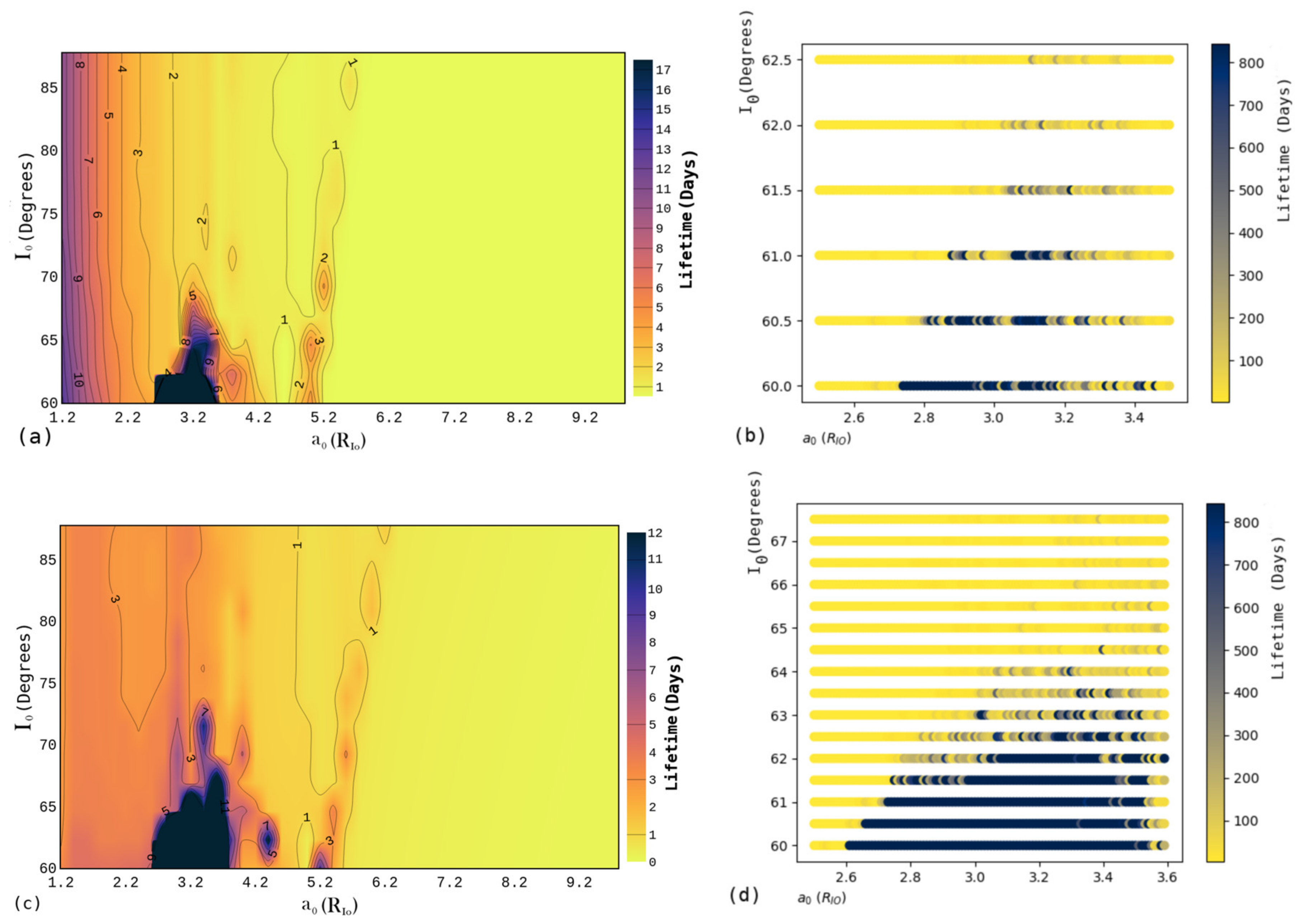
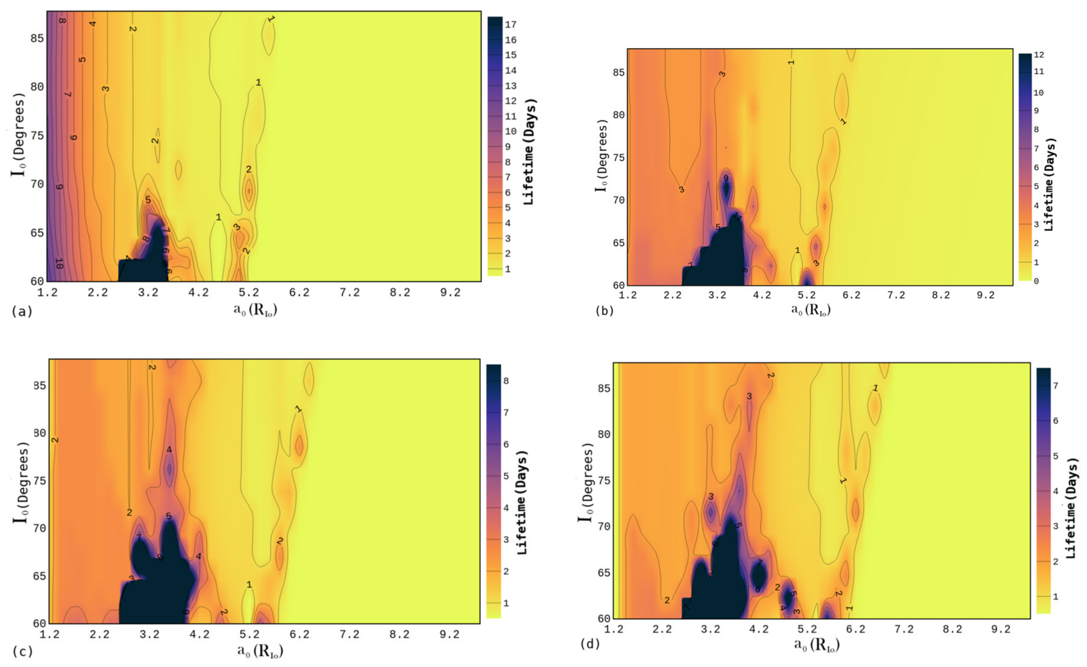
In Figure 1a,b, these maps show orbit lifetimes in terms of inclination and initial semi-major axis. These maps show the behavior of the lifetimes as a function of the initial conditions selected, considering that these orbits are initially circular. The results express that there is a semi-major axis region between and for inclinations between 60.0 and 62.5 degrees, as shown in the darker region in Figure 1a, in which it was observed that some orbits survived the total integration time. These conditions can be better observed in Figure 1b, where we show a zoom of this region. The neighboring orbits presented in this interval survive times between 18 and 831 days, as shown in Figure 1b. The other values of the initial semi-major axis and inclination combinations have orbits with lifetimes up to 17 days.
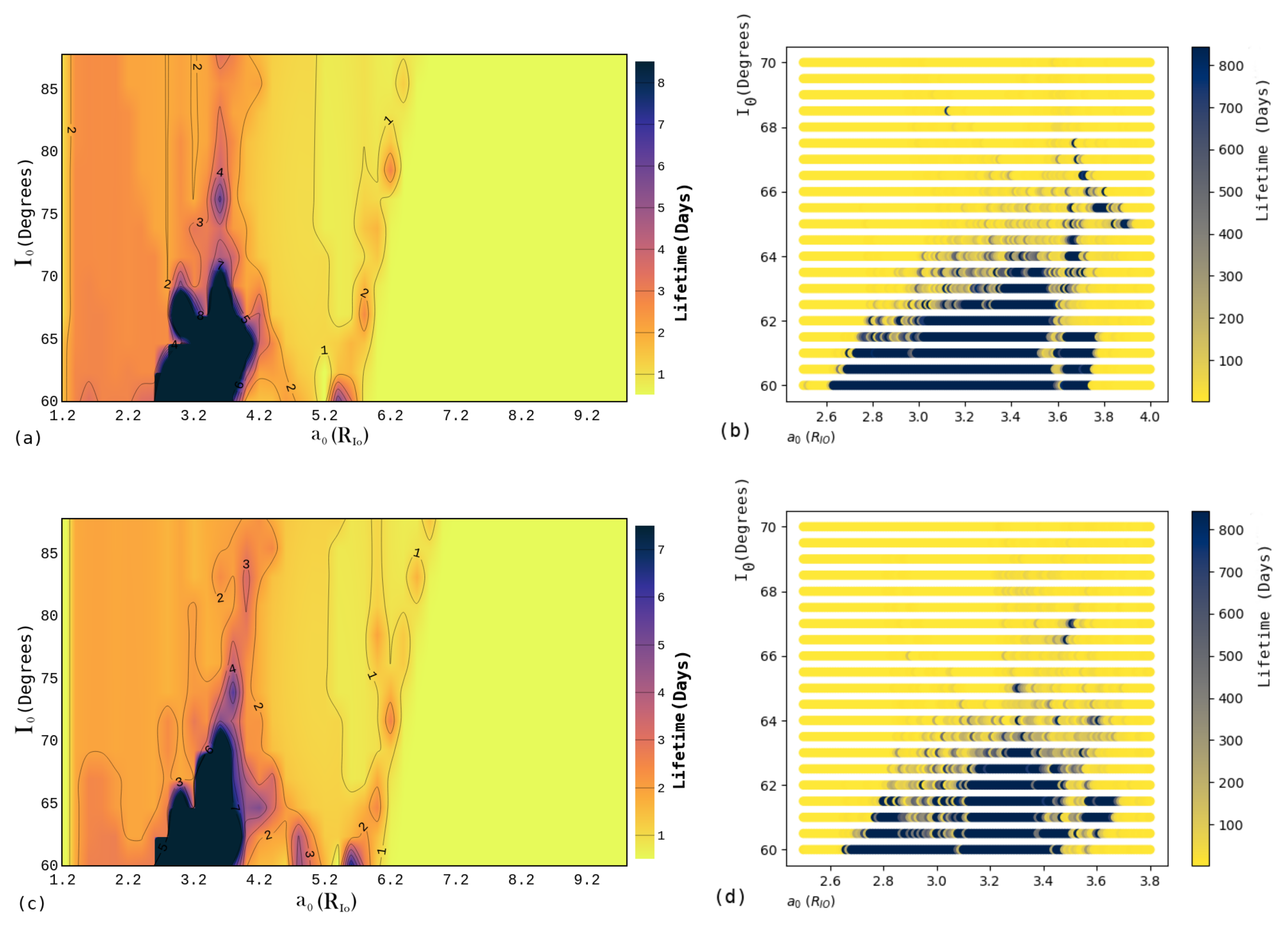
For the cases with initial eccentric orbits, for to , the results also showed similar behaviors. The darker regions in Figure 1c, Figure 2a,c correspond to regions where some orbits survive for the total integration time. As an example, in the case of , Figure 1c, the results show that this region lies in the range between and to the semi-major axis and an inclination interval of 60–67.5 degrees. For initial eccentric orbits with , as shown in Figure 2a, the best times obtained are in the range of the initial semi-major axis between and , and it covers the inclination range from 60 to 70 degrees. In terms of lifetimes, those orbits that did not survive the total time of integration of years; they lasted up to 824 days for , as shown in Figure 1d. For , we had orbits lasting between 10 and 816 days, as shown in Figure 2b, and orbits lasting up to 834 days, for , as shown in Figure 2d.
The analysis of the regions external to the interval show us that the lifetimes of these orbits have a great dependence on the choice of the initial semi-major axis and, consequently, the initial altitude of the probe. There is also a dependency on the choice of the initial inclination. This behavior can be explained considering that the orbits implemented with lower altitudes, with a semi-major axis between and , experience less gravitational perturbation of Jupiter. Thus, the probes placed closer to Io have longer orbit durations. Likewise, orbits implemented at higher altitudes, such as or higher, because they are further away from Io, suffer from more perturbative effects from Jupiter, which contributes to decrease the lifetime of the orbits. However, from the observed data, the best initial semi-major axis interval for placing the probes is in the range . Although this interval does not have the regions of lower initial altitudes analyzed, some initial conditions, as shown in Figure 1b–d, have orbits with adequate times for carrying out possible missions.
These results are important, because previous works [43,44] reinforce the results regarding the dependence of lifetimes with the choice of the initial semi-major axis around other natural satellites. In the case of orbits around Io, our maps show several initial conditions with lifetimes greater than 180 days, so evidencing orbits with good times for carrying out possible missions.
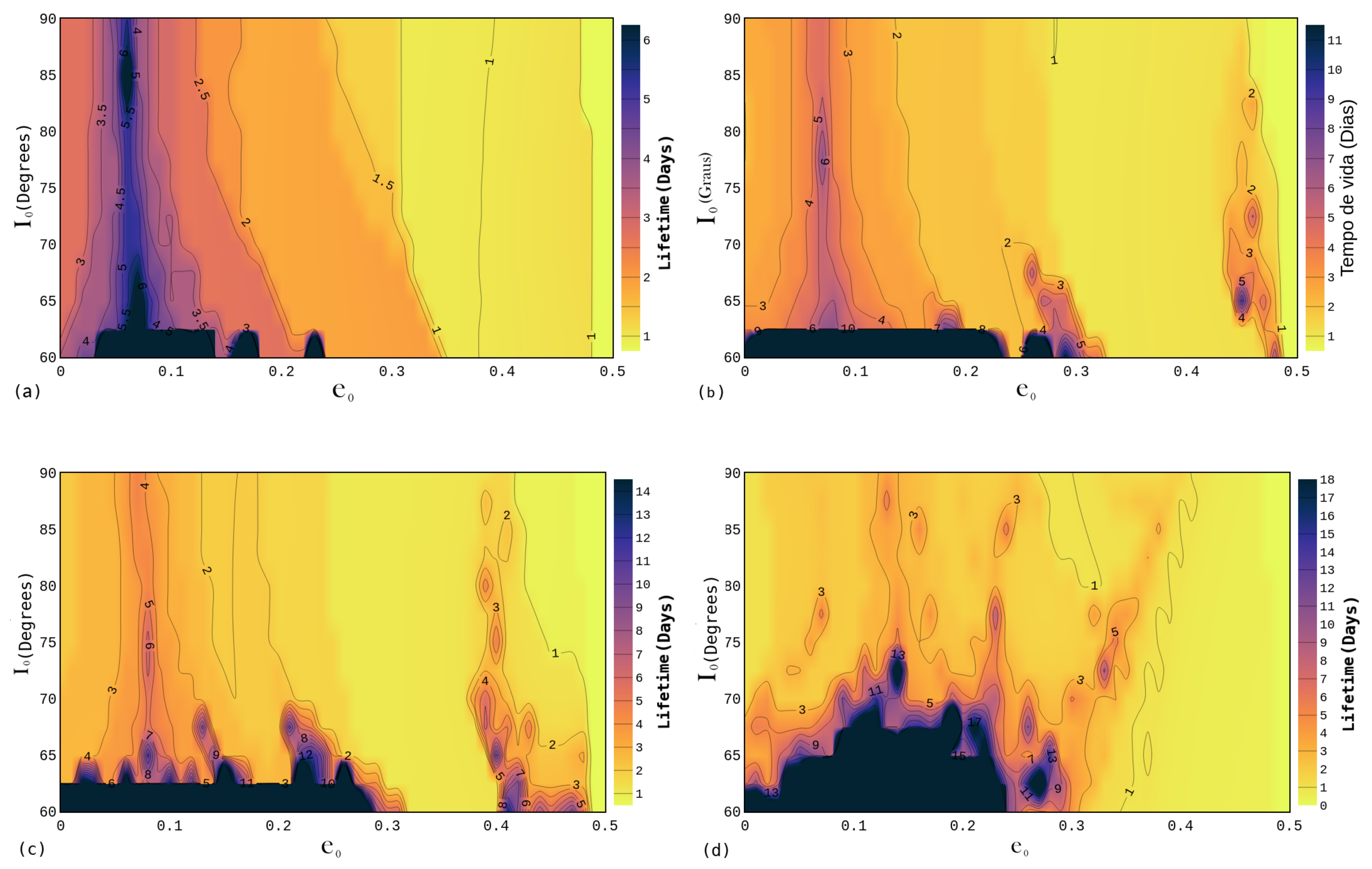
3.2. Analysis of Initials Inclination and Eccentricity
Regarding the analysis of the effects due to the choice of the initial inclinations and eccentricities, we perform simulations considering the values of , , , , , , and for the initial semi-major axis. These values of were based on the results obtained in Section 3.1, where we observe the effects due to the initial semi-major axis. The maps, as a function of the initial inclination and eccentricity of the orbit of the probe, are shown in Figure 3 and Figure 4.
The analysis of the results allowed us to observe that the lifetime of the orbits increases for lower values of inclinations in the range of 60–90 degrees. This behavior was also observed in previous works such as [16], which showed orbits around Io by considering the collision criterion through the study of the eccentricity of the orbit. This behavior of obtaining longer lifetimes for lower values of inclinations is related to the action of the Kozai–Lidov effect, since this effect tends to be more intense as the orbits are more inclined. Thus, orbits with smaller initial inclination feel less the action of the Kozai–Lidov effect. The coupling between the inclination and the eccentricity is not large, favoring the permanence of the probe for a longer time.
A more expressive constrain was observed with respect to the initial value of the eccentricity of the orbit. It was seen that longer lifetimes were obtained for lower values of the eccentricity. This is due to the fact that more eccentric orbits present an apoapsis closer to the third body. This proximity of the apoapsis to Jupiter produces a greater perturbation. Furthermore, the proximity of the periapsis of the orbit of the probe to the natural satellite favors the collision with the surface of Io.
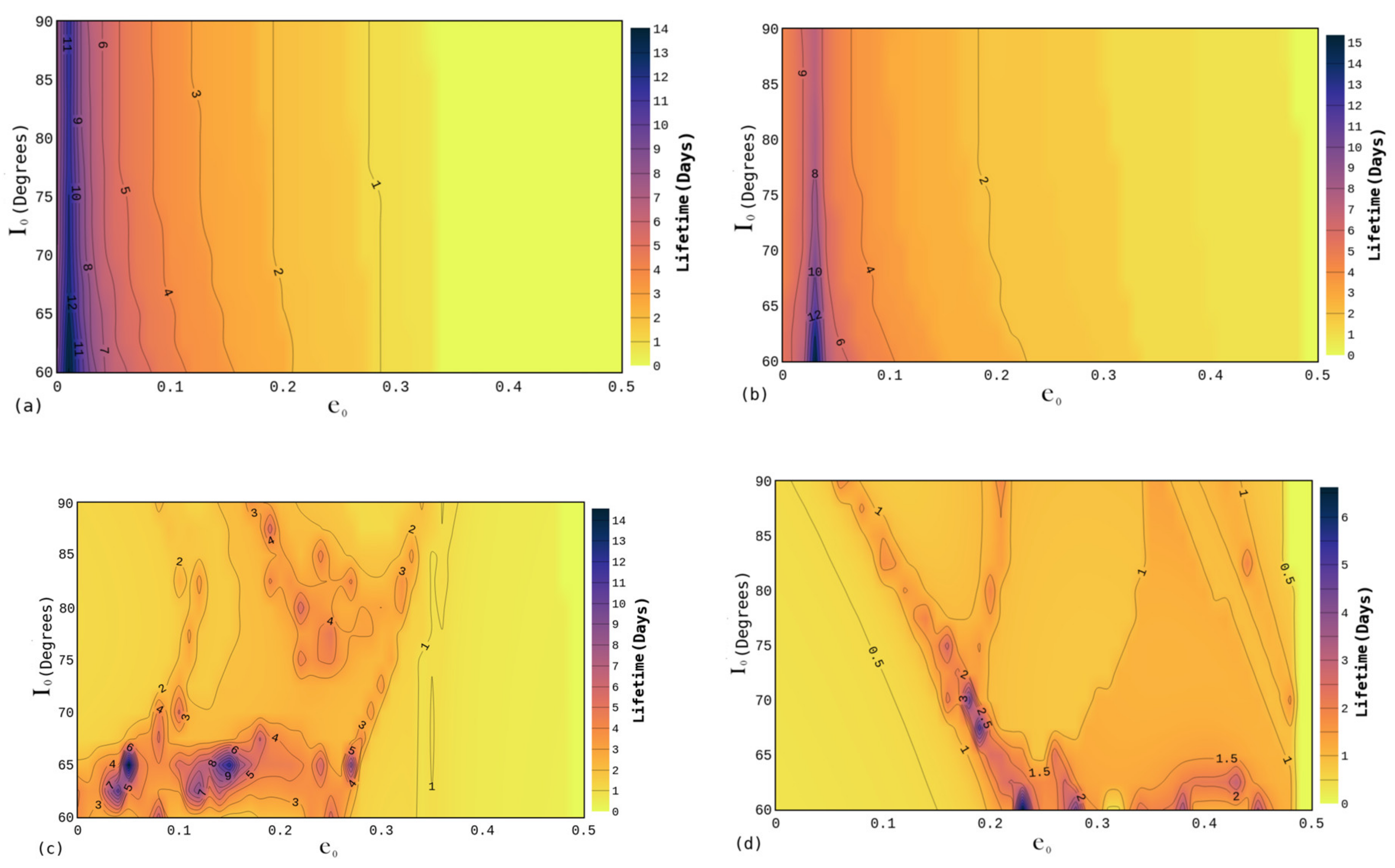
For the initial semi-major axis of , as shown in Figure 3a, these behaviors can be seen since longer lifetimes are in regions of smaller inclinations, 60 degrees, and circular orbits. However, the lifetimes of these orbits are no longer than 14 days. Likewise, the orbits implemented with an initial semi-major axis equal to , as shown in Figure 3b, did not also present orbits with a duration greater than 15 days. Orbits with longer times were located in regions of low inclination, 60 degrees, and for nearly circular orbits with . The maps in Figure 3c,d show the results for a semi-major axis of and , with orbits with maximum times of 14 and 6 days, respectively.
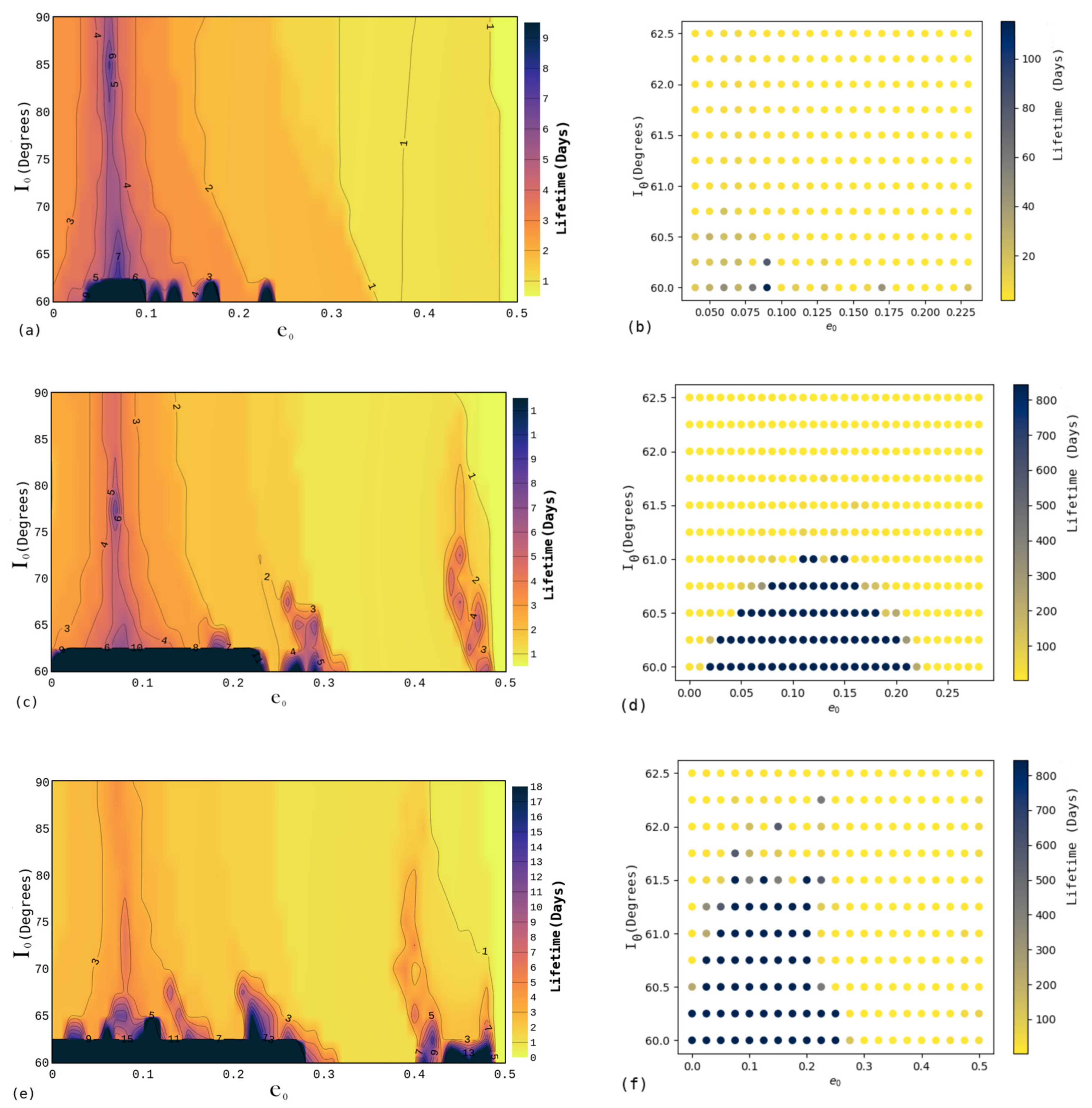
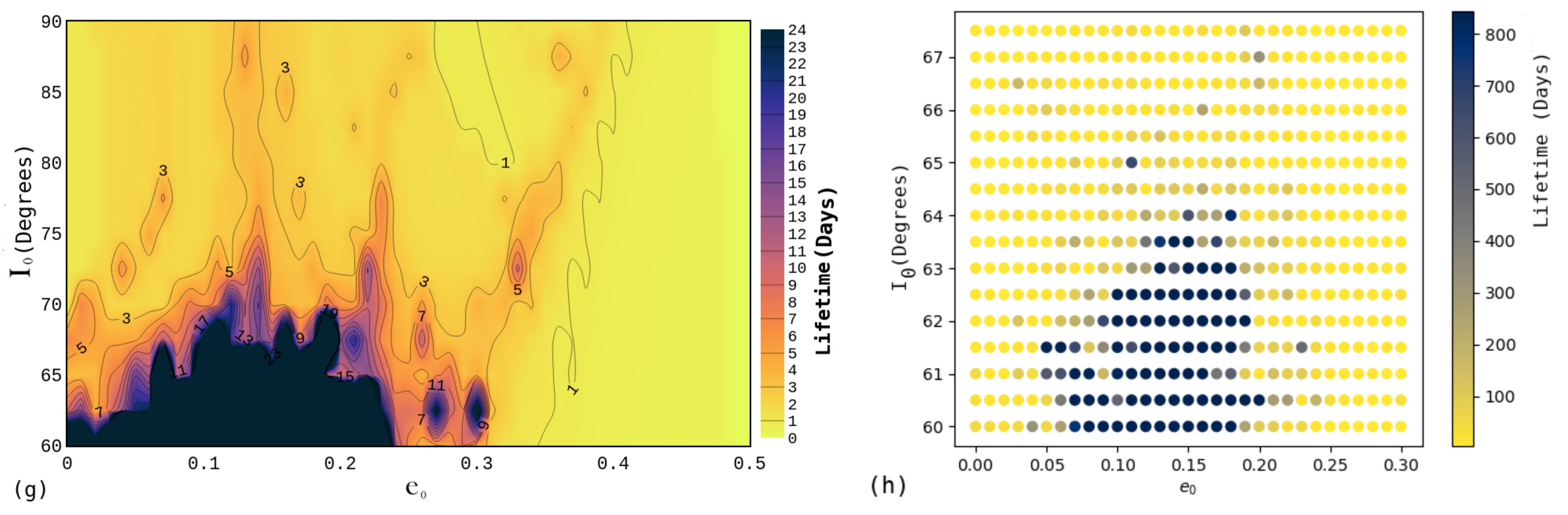
The general dependence on the initial inclination and eccentricity was also observed in maps generated with initial semi-major axes of and , as shown in Figure 4a,b, respectively. However, in these cases, some orbits with lifetimes longer than all their neighborhood were found. These regions are present in the map shown in Figure 4a, in the range of 0.04–0.09 for the eccentricity and inclination of 60 degrees, and for the conditions , , , , and also in the map of Figure 4b, for the range of 0.0–0.23 and when . For all conditions presented in Figure 4a,b, the initial inclination was assumed to be degrees.
The lifetimes for and , outside the appropriate orbital region, orbits with 9 and 11 days, respectively, have lifetimes that are very short in order to plan a mission. However, in some regions, orbits lasting between 11 and 115 days for were found, but no orbits survived for the full integration time, as shown in Figure 4b. However, in the case of orbits with , orbits were found in the darkest region, with lifetimes between 12 and 320 days, as shown in Figure 4d. For the initial altitude of , corresponding to , about 65 initial conditions of the probe survived during the total time of integration, which corresponds to at least years (844 days). These conditions can also be observed in Figure 4d. For both cases, and , there were no records of escapes from the region of interest.
For orbits initially with , most lifetimes are up to 18 days. However, for , orbits surviving during the full integration time were also located in the darkest region of the map. These surviving orbits were found in the range of initial eccentricities of 0.0–0.27 and initial inclination between 60 and degrees. A region with high eccentricity, near up to , with inclinations between 60.0 and 62.2 degrees, have orbits lasting up to 120 days, which are also located in the darker regions of the map (Figure 4a). However, not all orbits presented in these darker regions, those within 0.0–0.27 and close to survived the total integration time ( years). Around 12 ejections from the region of interest and more than 150 collisions were found. There are also cases, for both situations, with lifetimes in the range from 21 to 774 days (approximately 2 years), as shown in Figure 4c.
The results presented under the conditions of and are important because even in a region where the perturbations by Jupiter are strong, it was possible to find orbital conditions where disturbances were not large enough to eject or to make the probe collide with Io in a short period of time.
Orbits that survived the total integration time were also found with an initial semi-major axis equal to , Figure 4b,d. These orbits are among the conditions obtained in the range of for the initial eccentricity and inclination between 60 and degrees, and and . For both conditions, the initial inclination was degrees. In this range, orbits that collided with Io or escaped from the region of interest have lifetimes between 26 days and years.
Based on the results presented here, it was observed that in general, there is a relationship between the choice of the initial eccentricity and the lifetimes of the orbits. In this sense, orbits with lower values of the eccentricity tend to have longer lifetimes. This behavior is due to the fact that very eccentric orbits present a pericenter closer to Io, which may favor the collision. In addition, these orbits are more perturbed by Jupiter, which also contributes to possible collisions. The choice of inclination has also a certain degree of influence, because due to the Kozai effect [16], where there is an exchange between the value of the inclination and the eccentricity, the orbits tend to become eccentric, which favors possible collisions or escapes. These behaviors are faster when the probes have a higher value of inclination. The analysis of the maps in Figure 3 and Figure 4 also shows that the choice of the initial semi-major axis of the probe and, consequently, its altitude, plays an important role. Depending on the initial semi-major axis, a set of orbits with a sufficient lifetime to carry out a mission was found.
3.3. Analysis of the Initial Argument of Pericentre and Longitude of the Ascending Node
To understand the influence of the choice of the values of and , we performed numerical simulations considering some orbits that, in Section 3.1 and Section 3.2, were simulated with and equal to zero. We chose the orbits with longer lifetimes and those orbits that survived up to the total integration time. The simulations were performed using the data presented in Table 2, where the lifetimes are shown for those orbits with degrees and degrees.
Based on the orbits presented in Table 2, numerical simulations were performed keeping the values of , and for each case and varying the argument of pericenter and the initial longitude of the ascending node in the range of 0.0–360.0 degrees. The results are shown in Figure 5 and Figure 6.
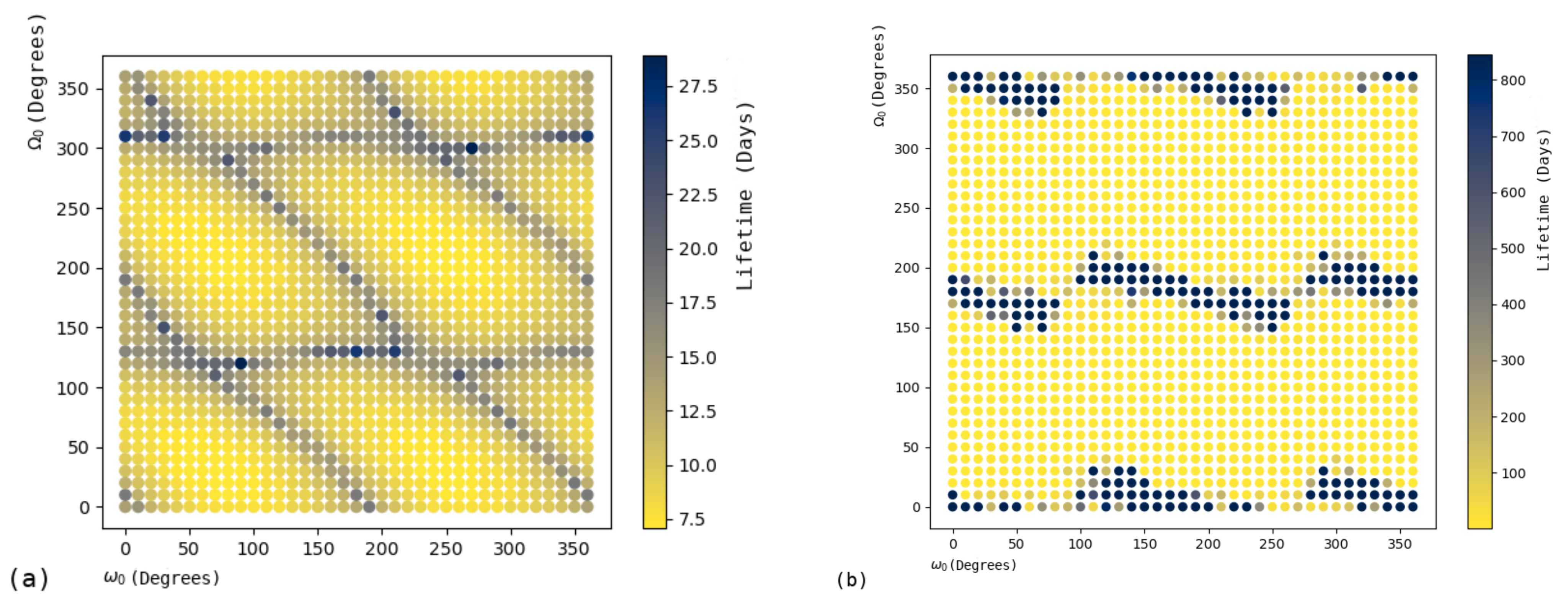
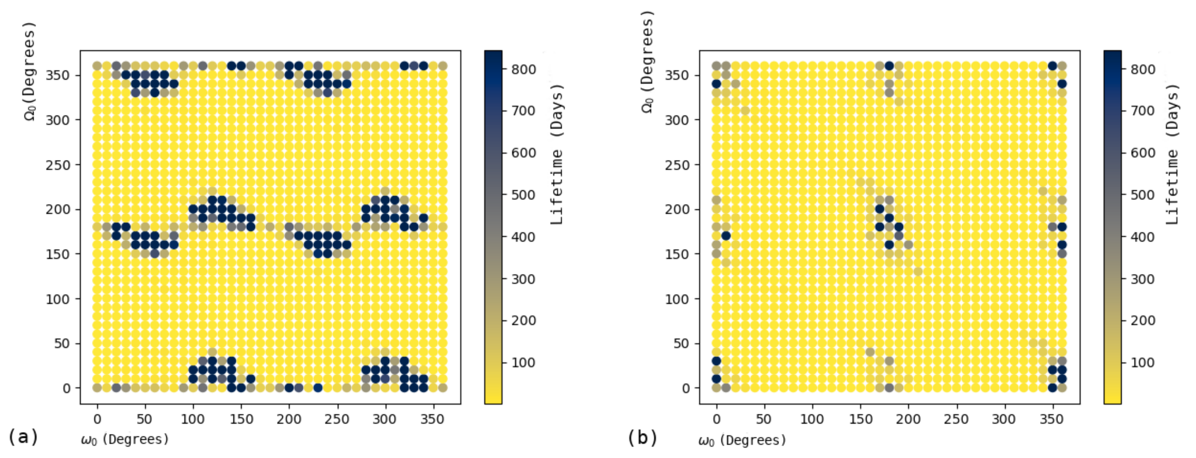
The results show that depending on the combination of and , the lifetimes of the orbits may increase or decrease compared to the cases assuming degrees and degrees. These gains and losses in the lifetimes were found in all simulated cases, as shown in Figure 5 and Figure 6. As an example, for degrees and degrees, as shown in Figure 5a, and degrees and degrees, as shown in Figure 6a, orbits with 28 and 789 days were found. This correspond to an increase of 14 and 560 days, respectively. In some cases, in the maps shown in Figure 5a and Figure 6b, it was possible to obtain orbits that survived during the total simulation time, years. Two examples can be seen in the interval of 350–360 degrees for the argument of the pericenter and longitude of the ascending node of 20 degrees in Figure 6b and the range of 140–150 degrees for the argument of pericenter and longitude of the node of degrees, as shown in Figure 5a.
However, it is important to mention that regarding the cases of orbits surviving the total integration time and the ones lasting 223 and 269 days, for degrees, significant decreases in the lifetimes were also found. These losses were so expressive, in all maps, where the orbits have only one day of duration. For the case shown in Figure 5b, these results correspond to a loss of up to 842 days. Thus, the results show the importance of properly choosing the value of the argument of the pericenter and the longitude of the node, since a successful implementation can generate orbits within the desired appropriate orbital region. Similar behaviors for and are also observed around other natural satellites, which can be seen in previous works ([25,43,44]).
3.4. Analysis of the Effect Due to the Non-Sphericity of Io—Zonal Harmonic
Considering the results obtained with the third-body perturbations due to Jupiter, we performed a set of numerical simulations including the perturbations of the non-sphericity of Io. Bibliographic references, such as [20,45,46], indicate that the central body flattening has the ability to compensate the effects due to a third body perturbation, helping to maintain some orbits that are stable, depending on the geometry of the system. Many of the results considering only the perturbations of Jupiter showed that many orbits around Io had a very short lifetime; only some intervals of the initial conditions contain orbits with large lifetimes. Therefore, the study of the effects of the flattening of Io is an option in the search for more stable orbits in addition to promoting a more complete approach to the mathematical model. Thus, based on [35], simulations were performed considering the value of for of Io. In our simulations, we only consider the effects of the coefficient , due to its greater magnitude compared to the other harmonics of Io. As an example, the value of is of the order of [35]. The simulations taking into account the effect of the of Io were performed, in some cases, for the same conditions simulated previously in the study of the initial inclination and eccentricity, initial inclination and semi-major axis, and for the study of the initial inclination and argument of pericenter and the longitude of the node. Table 3 shows the conditions.
Considering the results as a function of the inclination and the initial semi-major axis obtained only with the perturbations due to Jupiter and considering the perturbations due to Jupiter and the effects of of Io, as shown in Figure 7, we observe that the general behavior was maintained in all cases. Although the lifetimes had some changes, it is possible to see the same effects due to the choice of the initial inclination and semi-major axis observed in the maps of Figure 3 and Figure 4. It shows a larger dependence on the lifetimes with the choice of the initial semi-major axis and the initial altitude of the orbit. The appropriate orbital regions were also maintained in all maps, being generally present in the range of , for different inclination intervals. However, the regions already presented in the simulations only considering the perturbation from Jupiter are preserved.
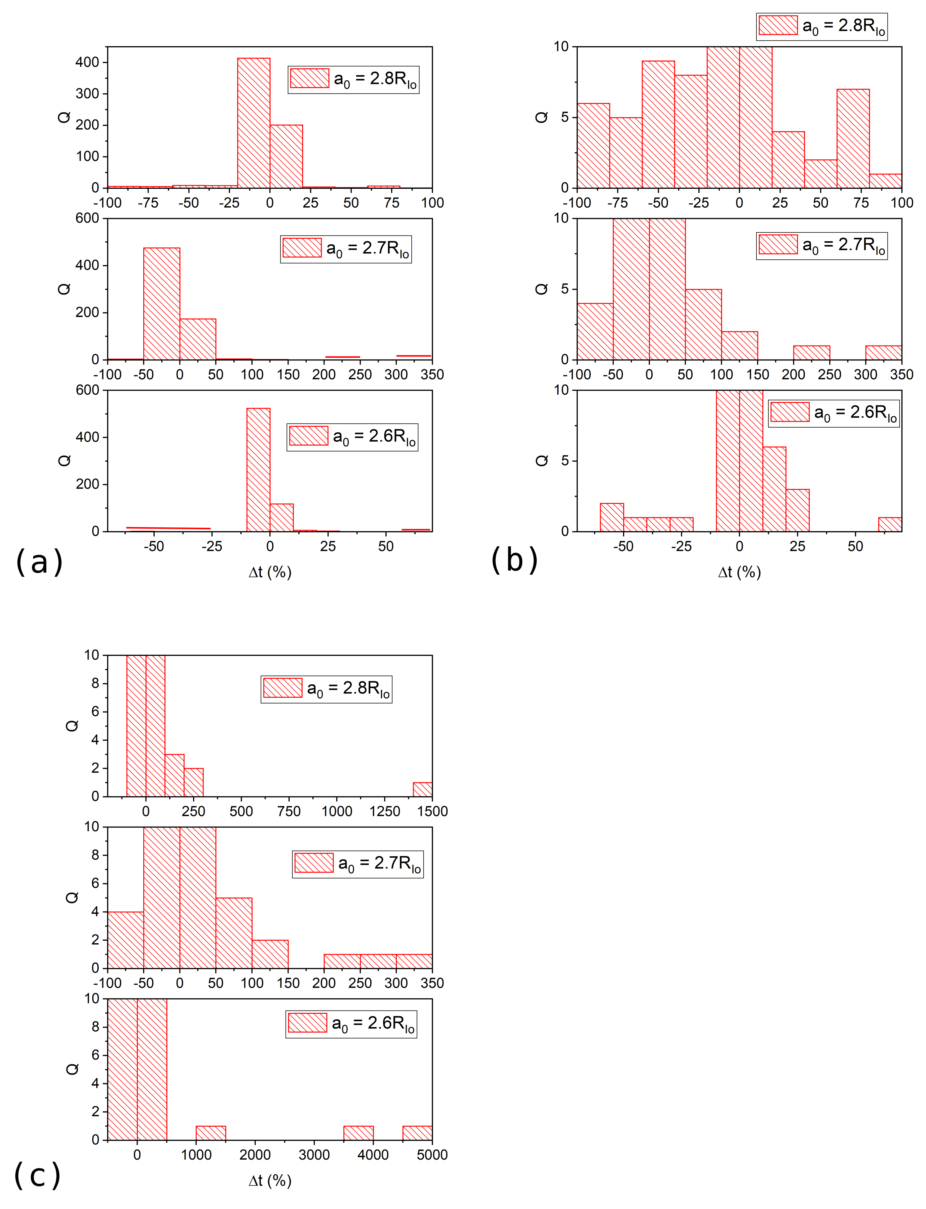
To study the effects due to the flattening of Io, the lifetime differences between each condition in the simulations with and without the effects due to were obtained. This result was represented by “”, in percentage. These data were organized in histograms of quantities of orbits by percentage of time variations in Figure 8. The positive percentages, placed on the horizontal axis, correspond to gains in the lifetimes of the orbits compared to the durations of the orbits without the term. The negative percentages represent losses in the lifetimes of the orbits in relation to the data obtained with only the effects from Jupiter perturbation. The results initially showed that the greatest gains and losses, due to the flattening effect of Io, were recorded in the region for the initial semi-major axis from to , while the differences for the other regions were not significant, since most of them were not larger than one day.
The results also showed that most orbits registered gains or losses between the range of 0 and , and that, in general, as the initial eccentricity increases, the number of orbits with lifetime losses increases. However, the orbits that registered some gain in the lifetime are still the majority, showing that the flattening of Io reduces the effects from Jupiter, even if in a few increments. One outstanding result was an orbit that achieved a gain between 4500 and 5000%. The initial conditions of this orbit were , and degrees, and its time without considering the effects due to of Io is only 5 days, while considering this effect is 251 days.
In the case of the maps in terms of the initial inclination and eccentricity, as shown in Figure 9, the same general behavior was observed, as in the case without the presence of . Therefore, we found orbits with longer lifetimes in the regions of low inclination and eccentricity. However, even though the behavior was maintained, the lifetimes registered a slight decrease, at least for the regions outside the appropriate orbital regions, which was shown as darker in the graphs. These regions of appropriate orbits continued to be present in all analyzed systems, except for and , where there were no occurrences.
The analysis of the maps and histograms in terms of and , for the initial semi-major axis of , and , identified several regions where the orbits within the duration desired for missions of interest were found, and it showed that when considering the effect of , most orbits showed reductions in the lifetime. However, these losses were up to in relation to the times considering only Jupiter perturbation. Orbital conditions with high gains were also obtained in these regions. For the case of , an orbit with a gain corresponding to , a lifetime increase from 5 to 251 days was found. Gains of up to were found for and up to for , as seen in Figure 10c.
The results for the maps as a function of the longitude of the ascending node and the initial argument of the pericenter, considering the flattening of Io, maintained the same behavior of the maps obtained when the perturbations were only from Jupiter. However, a small increase in the lifetime of the orbits was registered, where the largest amount of orbits is in the region of gains of up to . However, the simulation for and , with , was the one that registered the highest number of orbits where the lifetime decreases when considering the non-sphericity of Io. The losses are about . These results reinforce the importance of choosing the initial argument of the pericenter and the longitude of the ascending node, since it was seen that for certain regions, the flattening of Io reduces the duration of the orbits.
4. Conclusions
In our work, we investigated and mapped the best natural orbits with adequate durations to carry out space missions around Io. This lifetime has been established to be a minimum of 6 months. The studies showed the efficiency in the use of the collision detection method by checking the altitude as well as possible escapes by checking the energy of the system. The results are very important, because Io needs to be visited by an orbiter in the near future.
The orbits were searched as a function of the initial inclination and eccentricity, making it possible to identify appropriate orbital regions under different conditions for the initial semi-major axis. Orbits with lifetimes in the range of 6 months and years were found, which is an interval considered to be adequate for carrying out real missions.
In general, the orbits around Io suffer strong perturbations, given its proximity to Jupiter. Interesting orbits were found for , , and for the initial semi-major axis. Under these conditions, orbits lasting at least 844 days were found, always for lowest initial inclinations, and for initial eccentricities between 0.0 and 0.30. The simulations also showed orbits lasting between 31 and 774 days.
The general behavior of the simulations showed that as the initial orbital inclination was reduced, the lifetimes lasted longer as well as for less eccentric orbits. This behavior evidences that the Kozai effect is present in this region [16].
Simulations considering the initial orbit of the circular probe and with specific values of eccentricities were performed.
We also searched for the ranges of the initial semi-major axis that gives the longest lifetimes of orbits around Io. Our results showed that this range is located between and near . The extent of these regions, in terms of the choice of the initial inclination, varied with the initial eccentricity; however, it remained in the range of 60 to 67 degrees.
Our studies, based on the initial argument of pericenter and longitude of the ascending node, showed that a good choice of these initial elements can generate an increase in the lifetime of the orbits. However, attention should be paid to the fact that orbits that survive during the total time of integration or with high lifetimes are very sensitive to the choice of the initial argument of the pericenter and longitude of the ascending node, because small changes of a few degrees are enough to reduce the lifetime of the orbits in a few days.
The simulations considering the effects due to the flattening of Io allowed us to conclude that this effect is capable of reducing the effects of the third body in some cases. Most conditions ending in gains of time were found in the range of 5–40%. There were orbits with larger gains. Although these conditions were punctual, they are very important, because some orbits, considering only the effects of Jupiter perturbation, did not register durations greater than 180 days. Instead, they showed considerable gains considering the effect of , making these orbits last longer than 180 days. Among these orbits, we highlight the cases for , ; , ; , ; , ; , ; and , , all with degrees and , with degrees. These orbits had lifetimes of 5, 48, 19, 5, 14, 62, and 11 days, respectively, and they had an increase in the lifetime to 251, 240, 754, 250, 184, 217 and 168 days, respectively, when taking into account the effects due to .
However, not all initial configurations are favored by the effects of the flattening of Io. Losses were also found, and most of them were in the range of 5–25% compared to the system without . Losses of almost 99 % are rare, especially for cases where the probe was at lower altitude in relation to Io. Interestingly, the largest gains and losses were recorded in the same initial semi-major axis range of and .
Author Contributions
Conceptualization, T.C.F.C.F., A.F.B.A.P. and S.M.G.W.; methodology, T.C.F.C.F., A.F.B.A.P. and S.M.G.W.; software, T.C.F.C.F., A.F.B.A.P. and L.S.F.; validation, T.C.F.C.F. and L.S.F.; formal analysis, T.C.F.C.F., A.F.B.A.P., S.M.G.W. and L.S.F.; writing—preparation of original draft, T.C.F.C.F.; writing—review and editing, T.C.F.C.F., A.F.B.A.P. and S.M.G.W.; visualization, T.C.F.C.F., A.F.B.A.P. and S.M.G.W.; supervision, A.F.B.A.P. and S.M.G.W. All authors have read and agreed to the published version of the manuscript.
Funding
This work was supported by grant # 2016/24561-0, from São Paulo Research Foundation (FAPESP); grants # 309089/2021-2 and 313043/2020-5 from the National Council for Scientific and Technological Development (CNPq); and the Coordenação de Aperfeiçoamento de Pessoal de Nível Superior (CAPES). This paper has been supported by the RUDN University Strategic Academic Leadership Program.
Institutional Review Board Statement
Not applicable.
Informed Consent Statement
Not applicable.
Data Availability Statement
All data generated or analyzed during this study are included in this published article in the form of figures.
Acknowledgments
The authors thank Improvement Coordination Higher Education Personnel—Brazil (CAPES)—Financing Code 001. The Center for Mathematical Sciences Applied to Industry (Ce-MEAI), funded by FAPESP (grant 2013/07375-0) and the project 2016/23542-1 from FAPESP. SMGW thanks CNPq (Proc 313043/2020-5) for the financial support. This paper has been supported by the RUDN University Strategic Academic Leadership Program.
Conflicts of Interest
The authors declare that they have no conflict of interest with research institutions, professionals, researchers, and/or financial supports.
References
- Riedler, W.; Möhlmann, D.; Oraevsky, V.; Schwingenschuh, K.; Yeroshenko, Y.; Rustenbach, J.; Aydogar, O.; Berghofer, G.; Lichtenegger, H.; Delva, M.; et al. Magnetic fields near Mars: First results. Nature 1989, 341, 604–607. [Google Scholar] [CrossRef]
- Barth, C.A.; Pearce, J.B.; Kelly, K.K.; Wallace, L.; Fastie, W.G. Ultraviolet emissions observed near Venus from Mariner V. Science 1967, 158, 1675–1678. [Google Scholar] [CrossRef] [PubMed]
- Matson, D.L.; Spilker, L.J.; Lebreton, J.P. The Cassini/Huygens mission to the Saturnian system. In The Cassini-Huygens Mission; Springer: Berlin/Heidelberg, Germany, 2003; pp. 1–58. [Google Scholar] [CrossRef]
- Davies, A.G. Volcanism on Io; Cambridge University Press: Cambridge, UK, 2007; Volume 7. [Google Scholar]
- Pappalardo, R.T.; Belton, M.J.; Breneman, H.; Carr, M.; Chapman, C.R.; Collins, G.; Denk, T.; Fagents, S.; Geissler, P.E.; Giese, B.; et al. Does Europa have a subsurface ocean? Evaluation of the geological evidence. J. Geophys. Res. Planets 1999, 104, 24015–24055. [Google Scholar] [CrossRef]
- Carr, M.H.; Belton, M.J.; Chapman, C.R.; Davies, M.E.; Geissler, P.; Greenberg, R.; McEwen, A.S.; Tufts, B.R.; Greeley, R.; Sullivan, R.; et al. Evidence for a subsurface ocean on Europa. Nature 1998, 391, 363–365. [Google Scholar] [CrossRef] [PubMed]
- Parkinson, C.D.; Liang, M.C.; Hartman, H.; Hansen, C.J.; Tinetti, G.; Meadows, V.; Kirschvink, J.L.; Yung, Y.L. Enceladus: Cassini observations and implications for the search for life. Astron. Astrophys. 2007, 463, 353–357. [Google Scholar] [CrossRef]
- NASA. NASA’s Europa Clipper. 2021. Available online: https://europa.nasa.gov/ (accessed on 28 July 2021).
- Hofstadter, M.D.; Fletcher, L.N.; Simon, A.A.; Masters, A.; Turrini, D.; Arridge, C.S. Future Missions to the Giant Planets that Can Advance Atmospheric Science Objectives. Space Sci. Rev. 2020, 216, 1–17. [Google Scholar] [CrossRef]
- Turtle, E.; Barnes, J.; Trainer, M.; Lorenz, R.; Hibbard, K.; Adams, D.; Bedini, P.; Langelaan, J.; Zacny, K. Dragonfly: In Situ exploration of titan’s prebiotic organic chemistry and habitability. In Proceedings of the European Planetary Science Congress, Riga, Latvia, 17–22 September 2017; Volume 11. [Google Scholar]
- Peale, S.J.; Cassen, P.; Reynolds, R.T. Melting of Io by tidal dissipation. Science 1979, 203, 892–894. [Google Scholar] [CrossRef] [Green Version]
- Kozai, Y. The motion of a close earth satellite. Astron. J. 1959, 64, 367. [Google Scholar] [CrossRef]
- Kozai, Y. On the Effects of the Sun and the Moon upon the Motion of a Close Earth Satellite. SAO Spec. Rep. 1959, 22. Available online: https://adsabs.harvard.edu/pdf/1959SAOSR..22....2K (accessed on 28 July 2021).
- Kozai, Y. A new method to compute lunisolar perturbations in satellite motions. SAO Spec. Rep. 1973, 349. Available online: https://ntrs.nasa.gov/citations/19730008982 (accessed on 28 July 2021).
- Aksenov, E. The doubly averaged, elliptical, restricted, three-body problem. Astron. Zhurnal 1979, 56, 419. [Google Scholar]
- De Almeida Prado, A.F.B. Third-body perturbation in orbits around natural satellites. J. Guid. Control Dyn. 2003, 26, 33–40. [Google Scholar] [CrossRef]
- Domingos, R.; de Almeida Prado, A.B.; De Moraes, R.V. Studying the behaviour of averaged models in the third body perturbation problem. Proc. J. Phys. Conf. Ser. 2013, 465, 012017. [Google Scholar] [CrossRef] [Green Version]
- Gomes, V.M.; de Cássia Domingos, R. Studying the lifetime of orbits around Moons in elliptic motion. Comput. Appl. Math. 2016, 35, 653–661. [Google Scholar] [CrossRef]
- Domingos, R.C.; Prado, A.D.A.; De Moraes, R.V. A study of the errors of the averaged models in the restricted three-body problem in a short time scale. Comput. Appl. Math. 2015, 34, 507–520. [Google Scholar] [CrossRef]
- Dos Santos, J.C.; Carvalho, J.P.; Prado, A.F.; de Moraes, R.V. Lifetime maps for orbits around Callisto using a double-averaged model. Astrophys. Space Sci. 2017, 362, 227. [Google Scholar] [CrossRef] [Green Version]
- Cinelli, M.; Ortore, E.; Circi, C. Long lifetime orbits for the observation of Europa. J. Guid. Control Dyn. 2019, 42, 123–135. [Google Scholar] [CrossRef]
- Carvalho, J.; Elipe, A.; De Moraes, R.V.; Prado, A. Low-altitude, near-polar and near-circular orbits around Europa. Adv. Space Res. 2012, 49, 994–1006. [Google Scholar] [CrossRef]
- Carvalho, J.; Mourao, D.; Elipe, A.; De Moraes, R.V.; Prado, A. Frozen orbits around Europa. Int. J. Bifurc. Chaos 2012, 22, 1250240. [Google Scholar] [CrossRef]
- Carvalho, J.; Vilhena de Moraes, R.; Prado, A. Dynamics of artificial satellites around Europa. Math. Probl. Eng. 2013, 2013, 182079. [Google Scholar] [CrossRef] [Green Version]
- Carvalho, J.; Vilhena De Moraes, R.; Prado, A. Searching less perturbed circular orbits for a spacecraft travelling around Europa. Math. Probl. Eng. 2014, 2014, 529716. [Google Scholar] [CrossRef]
- Tzirti, S.; Tsiganis, K.; Varvoglis, H. Quasi-critical orbits for artificial lunar satellites. Celest. Mech. Dyn. Astron. 2009, 104, 227–239. [Google Scholar] [CrossRef]
- Costa, M.; Vilhena de Moraes, R.; Prado, A.; Carvalho, J. An optimization approach to search for quasi-critical inclinations for direct and retrograde orbits: Applications for artificial satellites around Io. Eur. Phys. J. Spec. Top. 2020, 229, 1429–1440. [Google Scholar] [CrossRef]
- Grasset, O.; Dougherty, M.; Coustenis, A.; Bunce, E.; Erd, C.; Titov, D.; Blanc, M.; Coates, A.; Drossart, P.; Fletcher, L.; et al. JUpiter ICy moons Explorer (JUICE): An ESA mission to orbit Ganymede and to characterise the Jupiter system. Planet. Space Sci. 2013, 78, 1–21. [Google Scholar] [CrossRef]
- Phillips, C.B.; Pappalardo, R.T. Europa Clipper mission concept: Exploring Jupiter’s ocean moon. Eos Trans. Am. Geophys. Union 2014, 95, 165–167. [Google Scholar] [CrossRef]
- Campagnola, S.; Buffington, B.B.; Petropoulos, A.E. Jovian tour design for orbiter and lander missions to Europa. Acta Astronaut. 2014, 100, 68–81. [Google Scholar] [CrossRef]
- Williams, D.A.; Keszthelyi, L.P.; Crown, D.A.; Yff, J.A.; Jaeger, W.L.; Schenk, P.M.; Geissler, P.E.; Becker, T.L. Volcanism on Io: New insights from global geologic mapping. Icarus 2011, 214, 91–112. [Google Scholar] [CrossRef]
- NASA. NASA’s Juno Mission Expands into the Future. 2021. Available online: https://www.nasa.gov/feature/jpl/nasa-s-juno-mission-expands-into-the-future (accessed on 28 July 2021).
- Murray, C.D.; Dermott, S.F. Solar System Dynamics; Cambridge University Press: Cambridge, UK, 1999. [Google Scholar]
- Neto, E.V.; de Almeida Prado, A.F.B. Time-of-flight analyses for the gravitational capture maneuver. J. Guid. Control Dyn. 1998, 21, 122–126. [Google Scholar] [CrossRef]
- Schubert, G.; Anderson, J.; Spohn, T.; McKinnon, W. Interior composition, structure and dynamics of the Galilean satellites. Jupiter Planet Satell. Magnetos. 2004, 1, 281–306. [Google Scholar]
- NASA. Soviet Lunar Missions. 2005. Available online: https://nssdc.gsfc.nasa.gov/planetary/lunar/lunarussr.html (accessed on 28 July 2021).
- Kosofsky, L.J.; El-Baz, F. The Moon as Viewed by Lunar Orbiter; US Government Printing Office: Washington, DC, USA, 1970; Volume 200.
- NASA. Lunar Orbiter 4. 2019. Available online: https://solarsystem.nasa.gov/missions/lunar-orbiter-4/in-depth/ (accessed on 28 July 2021).
- NASA. Lunar Orbiter 5. 2019. Available online: https://solarsystem.nasa.gov/missions/lunar-orbiter-5/in-depth/ (accessed on 28 July 2021).
- MacKenzie, S.M.; Neveu, M.; Davila, A.F.; Lunine, J.I.; Craft, K.L.; Cable, M.L.; Phillips-Lander, C.M.; Hofgartner, J.D.; Eigenbrode, J.L.; Waite, J.H.; et al. The Enceladus Orbilander Mission Concept: Balancing return and resources in the search for life. Planet. Sci. J. 2021, 2, 77. [Google Scholar] [CrossRef]
- Kozai, Y. Secular perturbations of asteroids with high inclination and eccentricity. Astron. J. 1962, 67, 591–598. [Google Scholar] [CrossRef]
- Park, S.Y.; Junkins, J. Orbital mission analysis for a lunar mapping satellite. In Proceedings of the Astrodynamics Conference, Scottsdale, AZ, USA, 1–3 August 1994; p. 3717. [Google Scholar]
- Xavier, J.; Prado, A.B.; Winter, S.G.; Amarante, A. Mapping Long-Term Natural Orbits about Titania, a Satellite of Uranus. Symmetry 2022, 14, 667. [Google Scholar] [CrossRef]
- Ferreira, L.S.; Sfair, R.; Prado, A.F.B.A. Lifetime and Dynamics of Natural Orbits around Titan. Symmetry 2022, 14, 1243. [Google Scholar] [CrossRef]
- Marchal, C.L. Fifth John V. Breakwell memorial lecture: The restricted three-body problem revisited. Acta Astronaut. 2000, 47, 411–418. [Google Scholar] [CrossRef]
- Liu, L.; Wang, X. On the orbital lifetime of high-altitude satellites. Chin. Astron. Astrophys. 2000, 24, 284–288. [Google Scholar] [CrossRef]
Figure 1.
Lifetime maps of initial orbits around Io as a function of initial inclination and semi-major axis for orbits with eccentricity, , equal to (a), , (c), , and (b,d) are zooms of the darkest region shown in (a,c), respectively. The numbers on the maps correspond to the lifetimes of the orbits for each region.

Figure 2.
Lifetime maps of orbits around Io, as a function of initial inclination and semi-major axis, for orbits with eccentricities, , equal to , (a), and , (c), and (b,d) are a zoom of the darkest region shown in (a,c), respectively. The numbers on the maps correspond to the lifetimes of the orbits for each region.

Figure 3.
Lifetime maps of orbits around Io, as a function of initial inclination and eccentricity, with semi-major axis, , equal to (a) , (b) , (c) and (d) . The numbers on the maps correspond to the lifetimes of the orbits for each region.
Figure 3.
Lifetime maps of orbits around Io, as a function of initial inclination and eccentricity, with semi-major axis, , equal to (a) , (b) , (c) and (d) . The numbers on the maps correspond to the lifetimes of the orbits for each region.

Figure 4.
Lifetime maps of orbits around Io, as a function of initial inclination and eccentricity, for orbits with semi-major axis, , equal to (a) , (c) , (e) and (g) , and maps of the darkest regions, for equal to (b) , (d) , (f) and (h) . The numbers on the maps correspond to the lifetimes of the orbits for each region.


Figure 5.
Lifetime maps of orbits around Io, as a function of the initial longitude of the node and argument of pericenter, (a) for the orbital condition (I) and (b) for the orbital condition (II) described in Table 2.
Figure 5.
Lifetime maps of orbits around Io, as a function of the initial longitude of the node and argument of pericenter, (a) for the orbital condition (I) and (b) for the orbital condition (II) described in Table 2.

Figure 6.
Lifetime maps of orbits around Io, as a function of the initial longitude of the node and argument of pericenter, (a) for the orbital condition (III) and (b) for the orbital condition (IV) described in Table 2.
Figure 6.
Lifetime maps of orbits around Io, as a function of the initial longitude of the node and argument of pericenter, (a) for the orbital condition (III) and (b) for the orbital condition (IV) described in Table 2.

Figure 7.
Lifetime maps of orbits around Io, as a function of initial inclination and semi-major axis, for orbits with initial eccentricity, , equal to (a), (b), (c) and (d), considering the effects of the flattening of Io. The numbers on the maps correspond to the lifetimes of the orbits for each region.

Figure 8.
Histograms of the percentage of gains or losses in the lifetimes considering simulations as a function of and for the initial semi-major axis values , and . The plot in (b) shows a clipping up to over the total histogram in (a). Each histogram has a fixed eccentricity for the entire simulation.

Figure 9.
Lifetime maps of orbits around Io, as a function of the initial inclination and eccentricity, for a fixed initial semi-major axis, considering perturbations due to the flattening of Io. The values of the semi-major axis is equal to in (a), equal to in (b), in (c) and in (d). The numbers on the maps correspond to the lifetimes of the orbits for each region.

Figure 10.
Histograms of the quantities of orbits, Q, by percentage of gains or losses in the lifetimes of the orbits as a function of and for the initial semi-major axis , and . The histograms in (b,c) zoom the total histogram showed in (a).
Figure 10.
Histograms of the quantities of orbits, Q, by percentage of gains or losses in the lifetimes of the orbits as a function of and for the initial semi-major axis , and . The histograms in (b,c) zoom the total histogram showed in (a).


Table 1.
Initial conditions used in the study of probes around Io (https://ssd.jpl.nasa.gov/, accessed on 10 June 2021 and [35]).
Table 1.
Initial conditions used in the study of probes around Io (https://ssd.jpl.nasa.gov/, accessed on 10 June 2021 and [35]).
| R (km) | a (km) | Sideral Time (Days) | ||
| Io | ||||
| () | (Degrees) | and (Degrees) | ||
| Probe | (0.0–0.5) | (60.0–85.0) |
Table 2.
Initial orbital conditions for the study of the choice of the longitude of the ascending node and the argument of the pericenter of the orbit of the probe. The lifetimes correspond to and equal to zero and degrees.
Table 2.
Initial orbital conditions for the study of the choice of the longitude of the ascending node and the argument of the pericenter of the orbit of the probe. The lifetimes correspond to and equal to zero and degrees.
| Orbit | Lifetime (Days) | ||
|---|---|---|---|
| a | |||
| b | |||
| c | |||
| d |
Table 3.
Initial orbital conditions of the orbits for the study of the choice of the longitude of the ascending node and the argument of the pericenter of the orbit of the probe. The lifetimes correspond to the case with and equal to zero.
Table 3.
Initial orbital conditions of the orbits for the study of the choice of the longitude of the ascending node and the argument of the pericenter of the orbit of the probe. The lifetimes correspond to the case with and equal to zero.
| (Degrees) | (Degrees) | (Degrees) | ||
|---|---|---|---|---|
| (0.0–0.5) | (60.0–90.0) | |||
| (0.0–0.5) | (60.0–90.0) | |||
| (0.0–0.5) | (60.0–90.0) | |||
| (0.0–0.5) | (60.0–90.0) | |||
| – | (60.0–90.0) | |||
| – | (60.0–90.0) | |||
| – | (60.0–90.0) | |||
| – | (60.0–90.0) | |||
| 80 | (0.0–360) | (0.0–360) | ||
| 90 | (0.0–360) | (0.0–360) | ||
| 80 | (0.0–360) | (0.0–360) | ||
| 80 | (0.0–360) | (0.0–360) | ||
| 80 | (0.0–360) | (0.0–360) |
Publisher’s Note: MDPI stays neutral with regard to jurisdictional claims in published maps and institutional affiliations. |
© 2022 by the authors. Licensee MDPI, Basel, Switzerland. This article is an open access article distributed under the terms and conditions of the Creative Commons Attribution (CC BY) license (https://creativecommons.org/licenses/by/4.0/).
Share and Cite
MDPI and ACS Style
Ferreira, T.C.F.C.; Prado, A.F.B.A.; Giuliatti Winter, S.M.; Ferreira, L.S. Mapping Natural Orbits around Io. Symmetry 2022, 14, 1478. https://doi.org/10.3390/sym14071478
AMA Style
Ferreira TCFC, Prado AFBA, Giuliatti Winter SM, Ferreira LS. Mapping Natural Orbits around Io. Symmetry. 2022; 14(7):1478. https://doi.org/10.3390/sym14071478
Chicago/Turabian StyleFerreira, Thamis C. F. Carvalho, Antonio F. Bertachini A. Prado, Silvia M. Giuliatti Winter, and Lucas S. Ferreira. 2022. "Mapping Natural Orbits around Io" Symmetry 14, no. 7: 1478. https://doi.org/10.3390/sym14071478
Note that from the first issue of 2016, this journal uses article numbers instead of page numbers. See further details here.