
Internal Similarity Network for Rejoining Oracle Bone Fragment Images


1
Key Laboratory of Oracle Bone Inscription Information Processing, Ministry of Education, Anyang 455000, China
2
School of Computer and Information Engineering, Anyang Normal University, Anyang 455000, China
*
Author to whom correspondence should be addressed.
Symmetry 2022, 14(7), 1464; https://doi.org/10.3390/sym14071464
Submission received: 14 June 2022
/
Revised: 11 July 2022
/
Accepted: 15 July 2022
/
Published: 18 July 2022
(This article belongs to the Special Issue Advances in Computer Vision, Pattern Recognition, Machine Learning and Symmetry)
Abstract
:Rejoining oracle bone fragments plays an import role in studying the history and culture of the Shang dynasty by its characters. However, current computer vision technology has a low accuracy in judging whether the texture of oracle bone fragment image pairs can be put back together. When rejoining fragment images, the coordinate sequence and texture features of edge pixels from original and target fragment images form a continuous symmetrical structure, so we put forward an internal similarity network (ISN) to rejoin the fragment image automatically. Firstly, an edge equidistant matching (EEM) algorithm was given to search similar coordinate sequences of edge segment pairs on the fragment image contours and to locally match the edge coordinate sequence of an oracle bone fragment image. Then, a target mask-based method was designed in order to put two images into a whole and to cut a local region image by the local matching edge. Next, we calculated a convolution feature gradient map (CFGM) of the local region image texture, and an internal similarity pooling (ISP) layer was proposed to compute the internal similarity of the convolution feature gradient map. Finally, ISN was contributed in order to evaluate a similarity score of a local region image texture and to determine whether two fragment images are a coherent whole. The experiments show that the correct judgement probability of ISN is higher than 90% in actual rejoining work and that our method searched 37 pairs of correctly rejoined oracle bone fragment images that have not been discovered by archaeologists.
1. Introduction
Approximately 3700 years ago, in the Shang dynasty of ancient China, the Chinese engraved characters on shells and bones. In modern times, approximately 156,000 fragments of shells and bones have been excavated from Yinxu, which was the capital of the Shang dynasty. The shells and bones have been named oracle bones and the characters engraved on them have been named oracle bone inscriptions. Rejoining oracle bone fragments plays an import role in studying the history and culture of ancient China and exploring the formation process of human characters, but the manual rejoining of so many oracle bone fragments is huge and inefficient work; therefore, oracle bone experts proposed the idea of rejoining oracle bone fragments by computer technology. However, traditional image-matching methods use the angle feature or template image to match fragment images, so they have a poor performance in rejoining oracle bone fragments because a corner may not exist in the oracle bone fragment edge [1], there may not be an overlap between two oracle bone fragment images or there may not be a general template image as a reference [2]. Therefore, traditional image-matching methods do not adjust to rejoin oracle bone fragment images.
Methods that rejoin object fragment images are summarized into two categories: local edge matching methods and deep learning methods for rejoining object fragment images. Many local edge matching methods have been given by researchers. For example, Kamran et al. [3] computed an inter-fragment matching boundary between each pair of fragments by solving the longest common sub-sequence (LCS), and a multi-piece alignment was used to prune incorrect matches and compose the final image. Zhang Q. et al. [4] gave a polygon feature-matching method to search spatial-adjacent fragment pairs, where the matching degree of each pair is measured by an improved local matching method for polygon features, and then a new path-generating method is given based on the matching angle. The multi-fragment reassembly is finally realized by generating a global path and reassembling the fragments according to the path. Liu et al. [5] proposed a longitudinal shredded paper method to achieve the splicing and restoration of broken paper by combining the information of a matching degree matrix and similarity matrix, which are calculated according to the continuity between texts. Zhang M. et al. [6] proposed a 2D fragment assembly method that uses the earth mover distance to measure a similarity based on length/property correspondence. It potentially matches a point on the first contour to a desirable destination point on the second contour, and a greedy algorithm is used for 2D fragment assembly by repeatedly assembling two neighboring fragments into a composite one. In summary, these methods require a high edge consistency of object fragments and are suitable for rejoining paper document edges, but are not suitable for rejoining an oracle bone fragment image with local missing edges.
Among deep learning methods for rejoining object fragment images, Paumard et al. [7] gave a shortest path optimization method that uses a neural network to predict positions of archaeological fragments, and a graph that leads to the best reassembly is made from these predictions. Le et al. [8] put forward a shredded image reassembly method that builds a convolutional neural network (CNN) to detect the compatibility of a pairwise stitching, and used it to prune computed pairwise matches; after that, they applied a boost training and loop closure algorithm to improve the network efficiency and accuracy. A Siamese network was proposed by Ngo T. et al. [9] by combining a residual network and spatial pyramid pooling to match excavated wooden fragment images. A fragment-matching approach based on pairwise local assemblies uses a 2D Siamese neural network [10] to evaluate the matching probabilities of Ostraca fragments; the network is designed to simultaneously predict the existence or absence of a match, and the spatial relationship of one fragment in relation to the other. Cécilia et al. [11] used a graph-neural-network-based solution to search pairwise patch information in order to assign labels to edge pairs representing the spatial relationships. This network classifies the relationship between a source and a target patch as being one of up, down, left, right or None; by doing so for all edges, the model outputs a new graph representing a reconstruction proposal. In summary, most of the above models provide a reorganization scheme of cultural relic fragments, and do not calculate the texture similarity of object fragments.
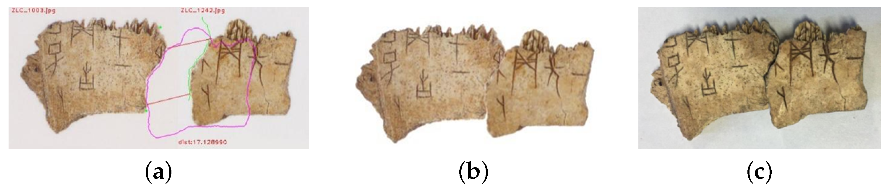
A current deep learning model, such as a detection model, includes a visual geometry group network, GooLeNet [12], regional convolution neural network [13,14] and YOLO [15]. A generative model includes a restricted Boltzmann machine and generative adversarial networks, a sequence model includes recurrent neural networks and long short term memory and a relational model includes a graph neural network and graph network [11,16]. Most of them are used for object detection and the classification or recognition of images, these applications belonging to the object segmentation or classification problem. However, rejoining fragment images belongs to the object connection or join problem, and the two problems belong to an inverse process. We assume that the deep learning model can be used to solve the rejoining problem of fragment images. In this paper, we focus on ideas from residual network architecture [17,18], gradient feature [19] and internal similarity [20,21,22] to improve the discrimination performance of an image-rejoining model and computer vision technology. Thus, an internal similarity network (ISN) is proposed to rejoin oracle bone fragment images. Our general scheme adopts a two-step method: the first step is to search matching edge segments; it does not use the corner feature yet, but it uses coordinate sequence features of edge segments (image EEM algorithm). The second step is to evaluate the similarity of image textures; we use gradient convolution features, and it has an advantage of computing the image continuity. Our current study in this paper enables computer vision technology to be applied to the actual rejoining work of oracle bone fragments, which was impossible before. The ISN model has a stronger adaptability, and we have used it to search dozens of new and rejoinable oracle bone fragment image pairs, which have been approved now and were not discovered by human archaeologists before. Figure 1 shows a whole image rejoined from an image pair, Figure 1a shows two matching edge segments of an image pair searched by EEM, Figure 1b shows a whole image rejoined by the target mask method and Figure 1c shows the rejoined physical oracle bone fragment.
2. Related Work
2.1. Rejoining Method Based on Local Edge Matching Algorithm
The design idea of the longest common sub-sequence (LCS) is as follows: the boundary curve of each fragment image is first extracted, and both of them are approximated with polygons; each segment of the boundary curve is represented by a descriptor, and the descriptor is calculated by color space and geometric coordinates; the LCS method is modified to find the sequence of the best matching segments; and the final transformation is computed to reassemble the fragment image. Our EEM algorithm uses geometric coordinates as a descriptor. It is similar to LCS, but the EEM algorithm does not use polygons to approximate the boundary curve, and it uses the intersection coordinates of circles and the edge as the descriptor. During matching edge segments, EEM does not consider color space information.
2.2. Residual Network Model
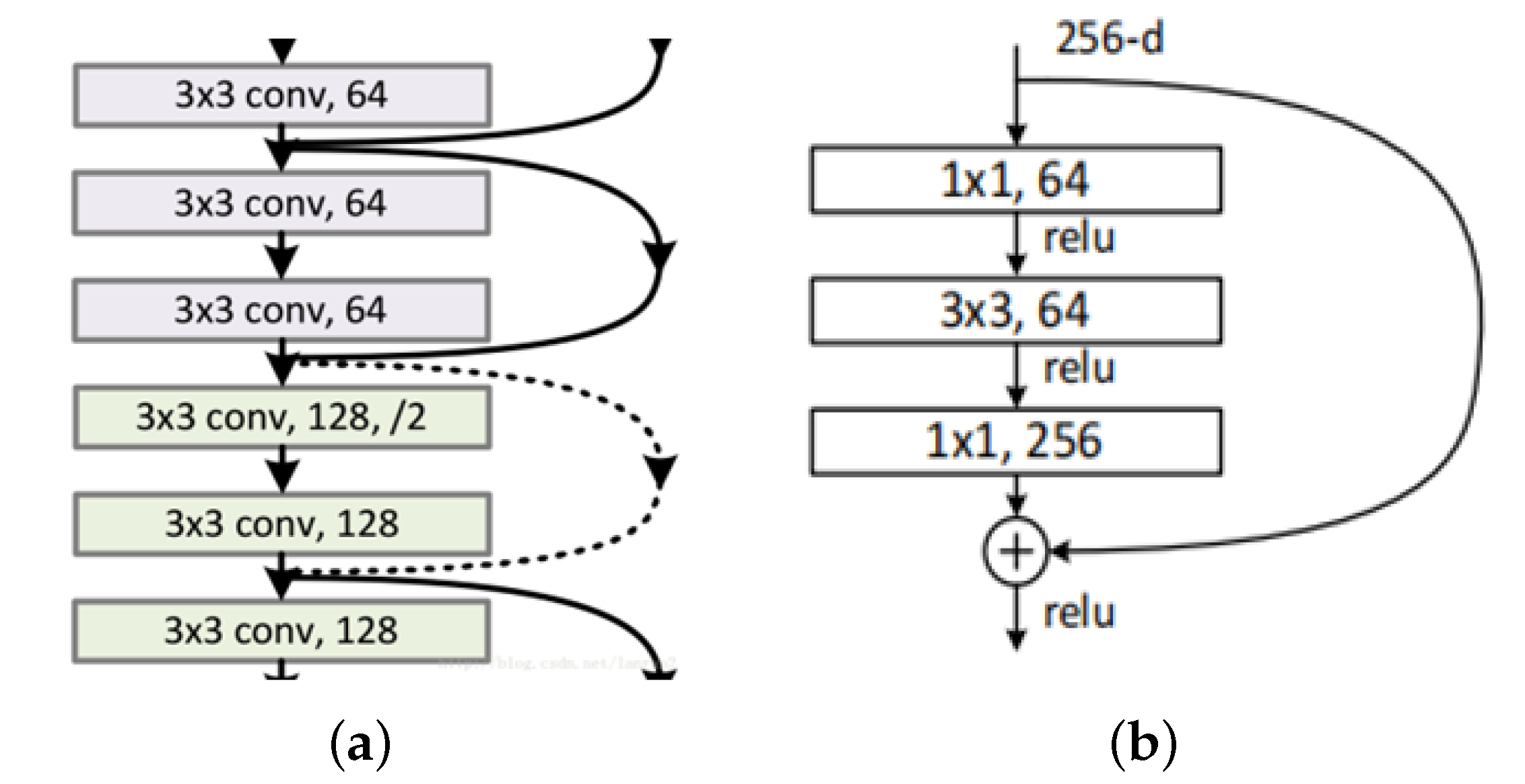
The edge-based method only gives a matching location in terms of geometry coordinates, but does not evaluate similarity, continuity or correlation regarding the color and texture of image pairs. Thus, combining the characteristics of rejoining a fragment image with the advantages of a residual network, a deep learning model is given to rejoin fragment images. In mathematical statistics, the residual error refers to the deviation between the actual observed value and fitted value. The coding residual vector is more effective than the coding original vector for vector quantization [19,20,21], so the residual network provides identity mapping and residual mapping to solve the gradient disappearance problem caused by an increasing depth. If the current network is optimal and the number of network layers continues to increase, the residual part would be close to 0, leaving only the identity mapping. Therefore, in theory, the residual network is always in the optimal state. As the dotted line shows in Figure 2a, in the residual network, 1 × 1 kernel convolution is used to project the identity mapping to the residual mapping space, and the operation’s target is to keep consistent data dimensions between identity mapping and residual mapping (Figure 2b) and to reduce the feature mapping dimension. In addition, the convolution kernel is usually added with a nonlinear activation function to make convolution features more recognizable.
In the model for rejoining the fragment image, we used the residual error between the actual observed value and fitted value to protect information integrity; at the same time, we calculated the residual vector among internal pixels in the convolution map of the local region image to achieve an internal similarity matrix of the local region image and to evaluate whether two fragment images are rejoinable or not [19]. Due to the fact that internal dissimilarity is related to horizontal and vertical gradient matrixes of the local region image, we defined the internal similarity of the local region image based on its intensity gradient along horizontal and vertical directions. The gradient plays an important role in presenting the image feature; for example, SIFT and SURF et. al, where most of them extract the feature by the image gradient in a multi-scale space, and the feature extraction and matching have a good performance in the destination location, recognition and scene splicing. In CNN, a frequently used method of calculating the gradient (such as Sobel, Prewitt and Roberts) applies a convolution kernel with a fixed size to slip on the image to accumulate products of the image pixels’ brightness and weight coefficients, inducing a large amount of computing work. Thus, this paper proposes a tensor slice dislocation subtraction method to calculate the gradient of image convolution feature mapping.
Supposing the mapping of a source convolution neural network is and its horizontal gradient is , then it is calculated by Equation (1), (W: width, H: height, F: Channels):
where S and D are slice maps of C, respectively, and they are calculated by the following equation horizontally (in Python code), where:
and .
Its vertical gradient is , and it is calculated by Equation (2):
where S and D are slice maps of C, respectively, and they are calculated by the following equation vertically, where:
and .
Its horizontal and vertical gradients are equivalent to the first order derivatives. Compared with tensor C’s dimension, the dimensions of tensor H and tensor V are reduced when computing the gradient; we used the padding function to make them equal, and then took the maximum value of tensor H and tensor V.
2.3. Image’S Internal Dissimilarity
Internal dissimilarity denotes the brightness difference between four nearest neighbors or eight nearest neighbors in the local region image; it denotes the maximum absolute value among three channels’ difference in pixel pairs, and the spatial relationship between two pixels can be indicated by their internal dissimilarity [18,19,20]. In the efficient graph-based image segmentation method given by Felzenszwalb et al [21], according to the maximum luminance difference value in an image region, the edge with the largest dissimilarity is defined in the minimum spanning tree. Among all of the edges connecting two regions, if the most similar places of the two regions or the smallest dissimilarity of edges (in the minimum spanning tree) was less than the intra dissimilarities of two regions, then the two regions can be merged. In segment-tree-based cost aggregation for stereo matching given by Mei et al. [22], cost aggregation coefficients of stereo matching are calculated by the dissimilarity of pixels in the image in order to construct the minimum spanning tree and complete the disparity calculation of binocular vision. This paper calculates the gradient matrix of a local region image to describe the relationship between neighbor pixels, and the matrix is used to make the residual feature location related.
3. Methodology
Four basic methods are proposed to locate matching edge segments and give an image similarity score:
- (1)
- Image edge equidistance matching (EEM) algorithm was applied to search matching edge segments in the oracle bone fragment image set.
- (2)
- Target-mask-based stitching method was proposed to put two images into a whole. The part of the whole image with matching edge segments, named the local region image (LRI), was cut from the whole image to extract the feature.
- (3)
- A convolution feature gradient map (CFGM) was designed to extract the texture feature of a local region image; it was embedded into a residual network to increase its stability.
- (4)
- An internal similarity pool (ISP) was given to compute the internal similarity of CFGM; after that, a full connection layer was used to give a score of the CFGM’s internal simialrity.
3.1. Local Edge Matching Algorithm
As shown in Figure 3a, our program drew the original oracle bone fragment image’s edge in green, and it drew the target oracle bone fragment image’s edge in pink. This paper gives two methods to locate the matching edge segments of two oracle bone fragment images: edge equal pixel matching algorithm and edge equidistance matching algorithm.
3.1.1. Image Preprocessing
When preprocessing oracle bone fragment image, we must pay attention to three aspects. Regarding the first aspect, it is necessary to select an edge segment from original image through human–computer interaction; the program could use the edge segment to search matching edge segments in any image set, the interaction meets pre-selection needs of expert and it is a welcome suggestion given by an archaeologist. Generally, when tracing image edge pixels, the pixel in the edge closest to X-axis is used as start position, and detector catches pixel coordinates anti-clockwise along image’s edge so that pixels of any image edge are stored in a list in form of coordinates anti-clockwise. In Figure 3a, the green downward arrow indicates that original image edge pixel coordinates were extracted anti-clockwise. Regarding the second aspect, if edge segments of two images can be rejoined, as the pink upward arrow shows in Figure 3a, the pixels’ coordinates sequence of one image’s edge must be set in reverse order; in this way, the local edge coordinate sequences of original and target images can maintain directional consistency. Our program reversed original image’s edge segment instead of target image’s edge segment to keep their directional consistency. It just needed to reverse once, and when searching matching edge segments in image set, target images’ edge segments did not need to be reversed, so the amount of calculation was reduced. Regarding the third aspect, it is necessary to keep the rotation invariance of an edge segment’s pixel coordinate sequence. The middle pixel of the edge segment of original image was taken as a center, the edge segment of the original image was rotated every 2 degrees and the degree variation range was set between [−20, 20] according to archaeologist’s suggestion; then, twenty-one rotated edge segments were achieved, as the blue curve segments show in Figure 3a. The middle pixel’s coordinates of the original image’s edge segment and any pixel’s coordinates of target image edge segment were used to calculate a translation vector; after that, twenty-one rotated local edges were shifted to target image’s edge, and the edge segment pixels in original and target images were sampled into two coordinate sequences, which were used as feature to match.
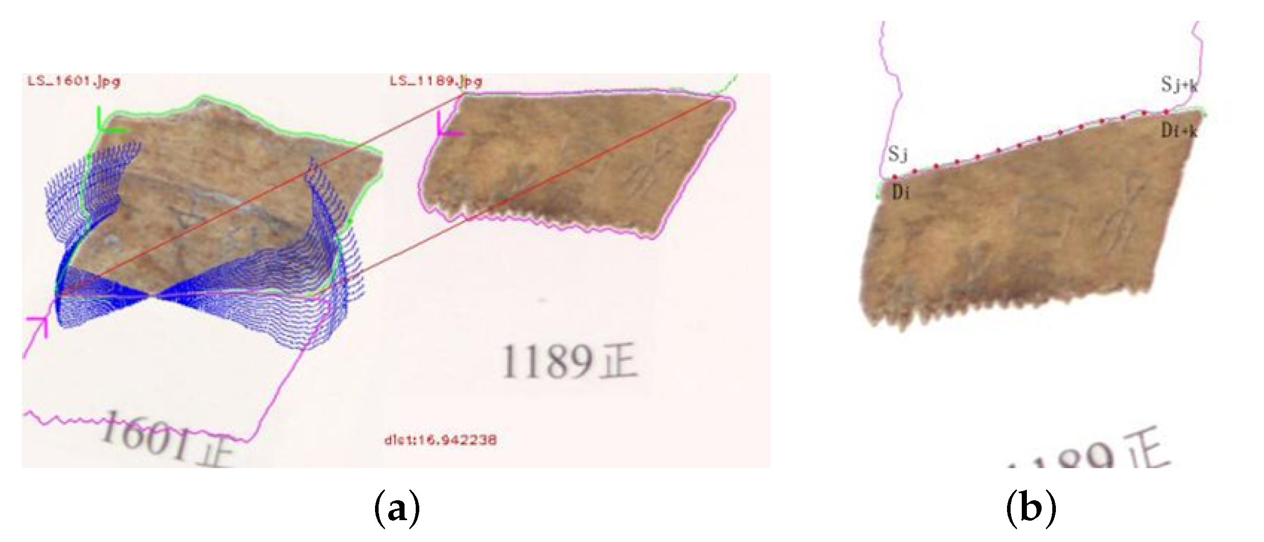
3.1.2. Image Edge Equal Pixel Matching Algorithm
For better understanding of image edge equidistance matching algorithm, first, this paper gives image edge equal pixel matching algorithm. In Figure 3b, to reduce the computation, when extracting pixels from original and target edge segments, we sampled one pixel every finite number of pixels, where the finite number could be set in our code. We calculated Euclidean distance between sampling pixels’ coordinates of original edge segment and target edge segment, and the distance was taken as dissimilarity to search matching edge segments. The minimum dissimilarity between original and target image local contours was used to predict whether two image can be rejoined or not. The length of matching edge segments was determined by the finite number and the number of sampling pixels: it must be less than the maximum length of matching edge segments. The edge segment between the first and last sampling pixels was similar to a sliding window; the twenty-one rotated edge segments of original image were compared with all edge segments of target image to find the location of the minimum distance between them. In Formula (3), denotes sampling pixels of original image edge segment, j denotes the subscript of the first matching sampling pixel in the pixel coordinate sequence of the original image edge segment, denotes sampling pixels of the target image’s edge segment, i denotes the subscript of the first matching sampling pixel in the edge segment coordinate sequence of the target image, denotes sum of the distance between the sampling pixels of the original and target images edge segments and k denotes the number of sampling pixels. If the minimum distance between original image edge segment and target image edge segment is less than the threshold T, the edge segments of the two images are matching at this location.
3.1.3. Image Edge Equidistance Matching Algorithm
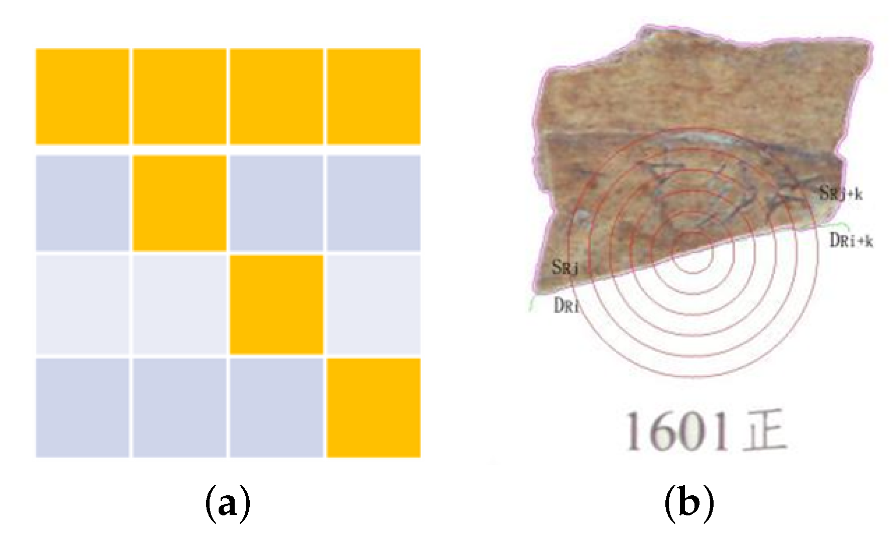
As shown in Figure 4a, if the same four pixels (yellow squares) are arranged obliquely or horizontally, the distances between the head and tail pixels would not be equal in different arrangement modes. Image edge equidistance matching (EEM) algorithm was proposed to solve the problem where the numbers of image edge pixels are the same but the distances are not equal in different arrangement modes.
As shown in Figure 4b, when candidate edge segment of the original image was rotated and translated to the edge of the target image, the intersections of the circles (with the same center and the radius increasing in equidistance every time) and the candidate edge segment were extracted as sampling pixels, which were used to calculate the sum of the distances between consistent coordinates of sampling pixel sequences from original and target image edge segments. The result was used as dissimilarity to judge whether two edge segments are matching. The length of matching edge segments was determined by the number of sampling pixels and the equidistance of the radius increased every time. In Formula (4), denotes sampling pixel of original image’s edge segment, Rj denotes the subscript of the first matching sampling pixel in the edge coordinate sequence of the original image, denotes sampling pixel of target image’s edge segment, refers to the sum of the distances between the corresponding sampling pixels at the two edge segments and is calculated by the EEM algorithm and k denotes the number of sampling pixels. EEM algorithm can skip the missing intermediate part in an edge segment, so it has strong adaptability.
3.1.4. Image Rejoining Method
After locating matching edge segments of original and target images, the two images need to be rejoined into a whole. In this paper, a mask-based stitching method was proposed to assemble the two images into a whole under condition that their edge segments have matching pixels’ coordinates sequence. Firstly, the rejoined image was defined by a size of (, ), the whole image’s size was calculated according to eight numbers, as shown in Formulas (5) and (6), respectively, and the eight numbers were , , , , , , and , respectively. (, ) denote the coordinates of the middle pixel of original image’s edge segment in the original image coordinate system, (, ) denote the coordinates of the middle pixel of the target image’s edge segment in the target image coordinate system, the original image is size of (, ), and denote its height and width, respectively, the target image is size of (, ) and and denote the target image’s height and width.
where and .
where and .
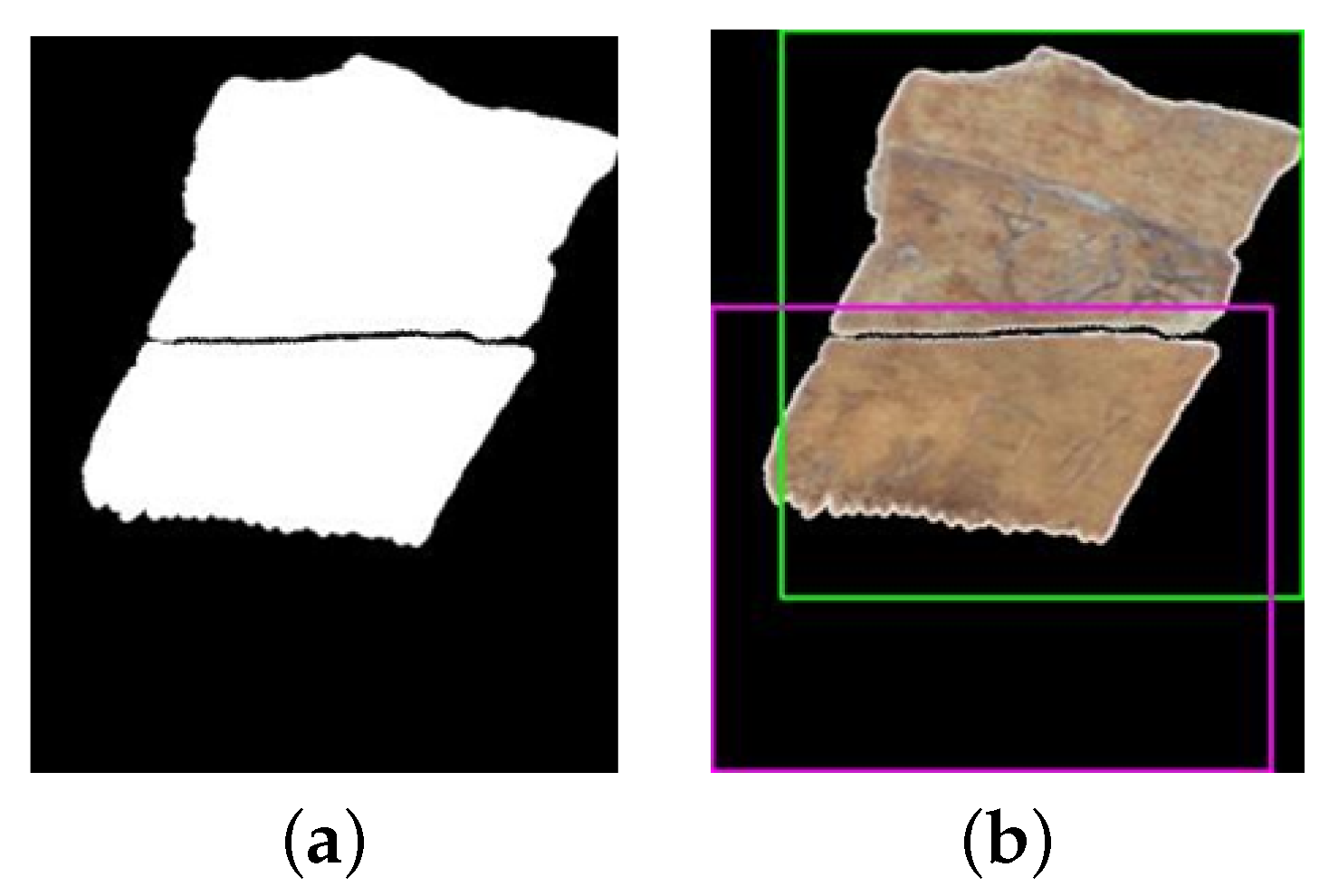
As shown in Figure 5a,b, regarding the mask-based rejoining method of oracle bone fragment image, firstly, supposing the rejoined image has a size of (, ), we achieved the binary image of original image and its size (the green box’s size in Figure 5b), and the original image was translated and rotated into the green box of the rejoined image according to the matching edge segments; similarly, according to the binary image of target image, its size (the pink box’s size shown in Figure 5b) and the matching edge segment, the target image was copied to the pink box’s location of the rejoined image by the mask, and, after these operations, a whole image was assembled by two oracle bone fragment images.
3.2. General Scheme
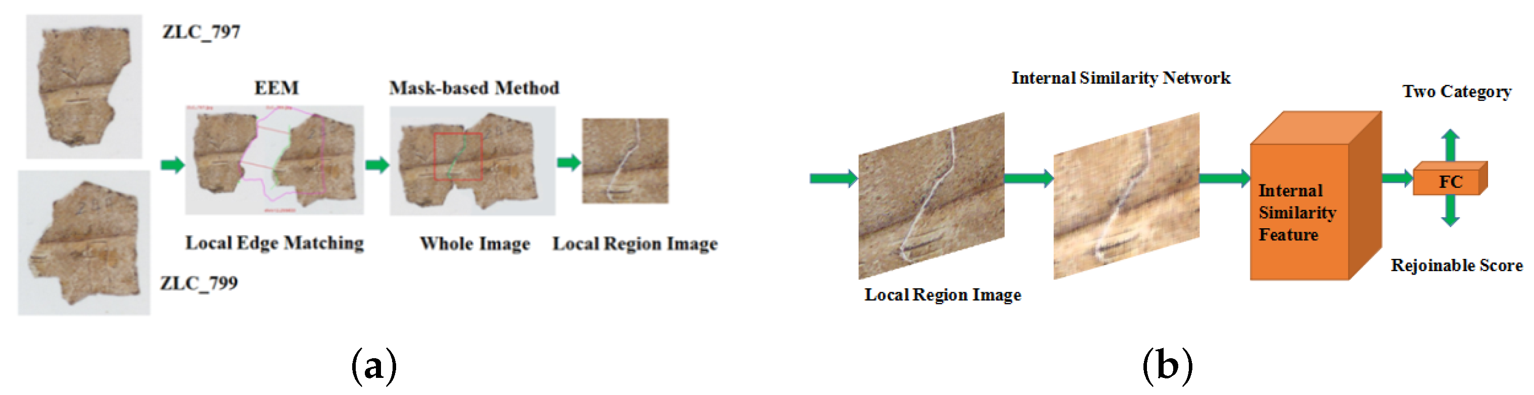
A general scheme is designed in this paper. In Figure 6a, before searching matching edge segments, an edge segment (the curve between two green points) should be selected from original image through human–computer interaction, and EEM algorithm was used to search any image set to find its matching edge segments. In Figure 6a, the original image is ZLC_797, and EEM algorithm searches a matching edge segment of target image numbered ZLC_799. Two matching edge segments that were marked between parallel lines were detected by image EEM algorithm; after that, the mask-based rejoining method put the original and target images together into a whole image, and a red box was given to cut local region image from the whole image. In Figure 6b, after achieving local region image, the residual network (improved by CFGM and ISP) was used to evaluate the similarity score of the convolution feature gradient map, and it was named internal similarity network (ISN). The gradient map was set between 7 × 7 convolution layer and maximum pooling layer in ResNet50, and internal similarity pooling (ISP) was used to replace the average pooling layer in the ResNet50. Softmax activation function, Glorot initial network model and adaptive momentum evaluation method were used to optimize the model.
3.3. Internal Similarity Pooling
Residual network does not calculate the similarity between adjacent pixels in the image, and the convolution feature does not have position correlation; as a result, it has a low accuracy in judging whether the oracle bone fragment image can be assembled together. This paper proposes internal similarity pooling (ISP) to calculate similarity feature of adjacent pixels in local region image. ISP makes convolution feature location-dependent by calculating similarity of adjacent position in local region image convolution map. The gradient map of convolution feature was set between 7 × 7 convolution layer and maximum pooling layer, and it was calculated by horizontal gradient (H) and vertical gradient (V).
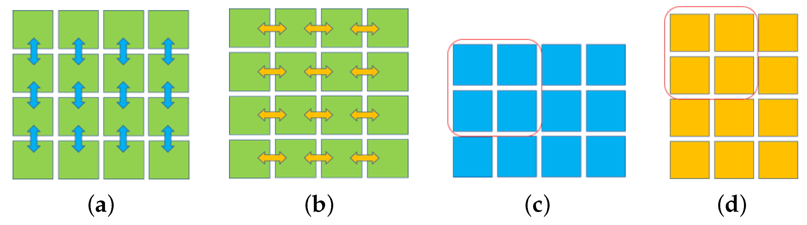
In ResNet50, a tensor size of 4 × 4 × 2048 was calculated at second to last layer, and it was reset to be of size 2 × 2 × 2048 by the average value pooling layer. In addition, the flattened tensor was put into full connection layer. As can be seen in Figure 7a,c, the tensor had a size of 4 × 4 in 2048 channels, the vertical subtraction method was used to calculate the gradient of two adjacent rows of each channel, and by obtaining the vertical gradient of 4 × 3, as shown in Figure 7b,d, the gradient of two adjacent columns was calculated by horizontal subtraction to obtain a 3 × 4 horizontal gradient. The vertical gradient data size of 4 × 3 was processed by a maximum pooling size of 2 × 2 and stride of 2 × 1; then, a vertical gradient tensor size of 2 × 2 × 2048 was achieved. The horizontal gradient data size of 3 × 4 was processed by a maximum pooling size of 2 × 2 and stride of 1 × 2; then, horizontal gradient tensor size of 2 × 2 × 2048 was achieved. The horizontal and vertical gradient tensors were used to calculate the similarity of horizontal pixels and vertical pixels [22]; the calculation method of similarity is shown in Formula (9), where e refers to the calculation of exponential power, d is the gradient difference in pixels, is harmonized parameter, / denotes division operation and ISP calculates the similarity based on the gradient tensor and the adjacent pixels in slip window, where the maximum similarity in the slip window is used as .
4. Experiment Verification
4.1. Experiment Platform and Dataset
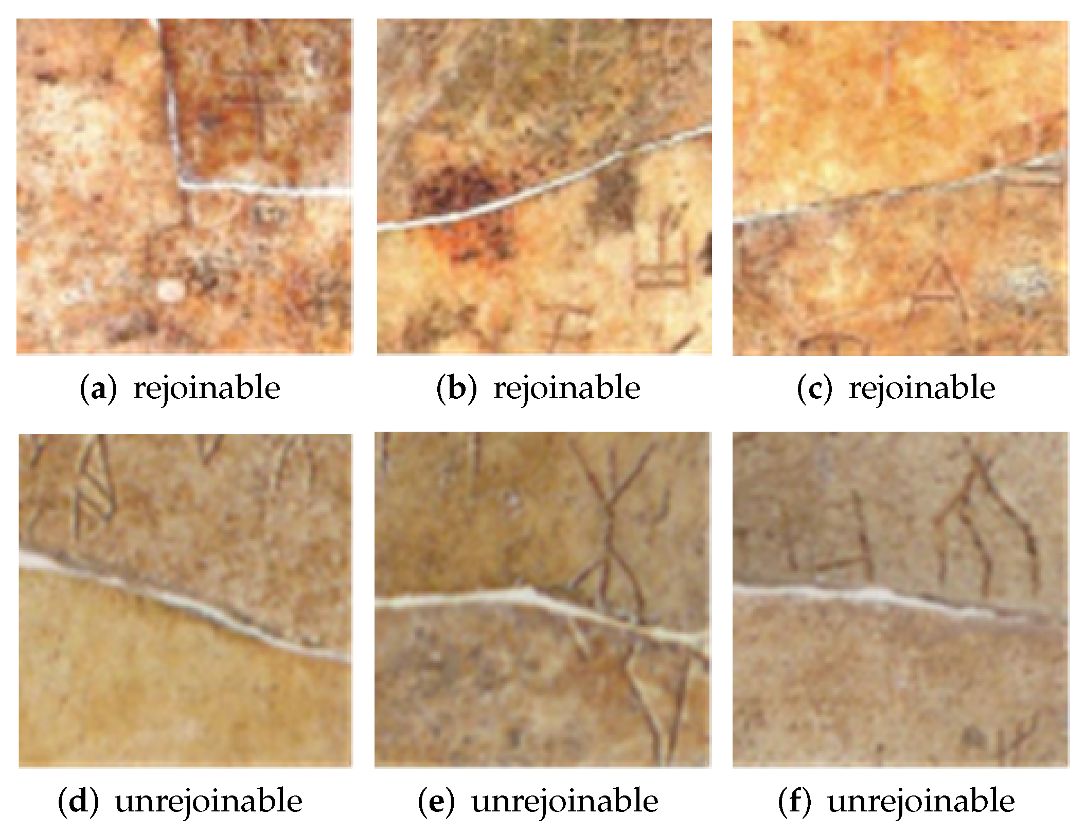
The experiment used the Ubuntu operating system (16.04), pycharm software development platform (2021.3.2), GeForce RTX 208, Anaconda3.0, python3.7, cuda 10.1, tensorflow 2.0.4 and opencv-python3.4.6. Oracle bone fragment image sets were obtained by scanning oracle bone description books, and the scanner’s type was Tengdahanlong OS12002. In this paper, we established a positive and negative sample image set of a local region image of an oracle bone fragment; the image set includes approximately 116,000 unrejoinable local region images that were achieved by the EEM algorithm from the ZLC oracle bone fragment image set (from institute of history of the Chinese Academy of Social Sciences), and it includes 23,000 rejoinable local region images that were cut from the Bingbian, Huadong image set et al. [23]. The train set and test set account for 75% and 25% of the whole data set, respectively, as shown in Figure 8. There are three local region images size of 121 × 121 in the first row, which are rejoinable images; there are three local region images in the second row, which are unrejoinable images. The effectiveness of various deep learning models were tested in this paper; when training the models, the size of the local region image was adjusted according to the input requirement, and each model was trained iteratively to ensure the convergence of network parameters.
4.2. Experimental Effect and Analysis
4.2.1. Performance of Edge Equidistance Matching
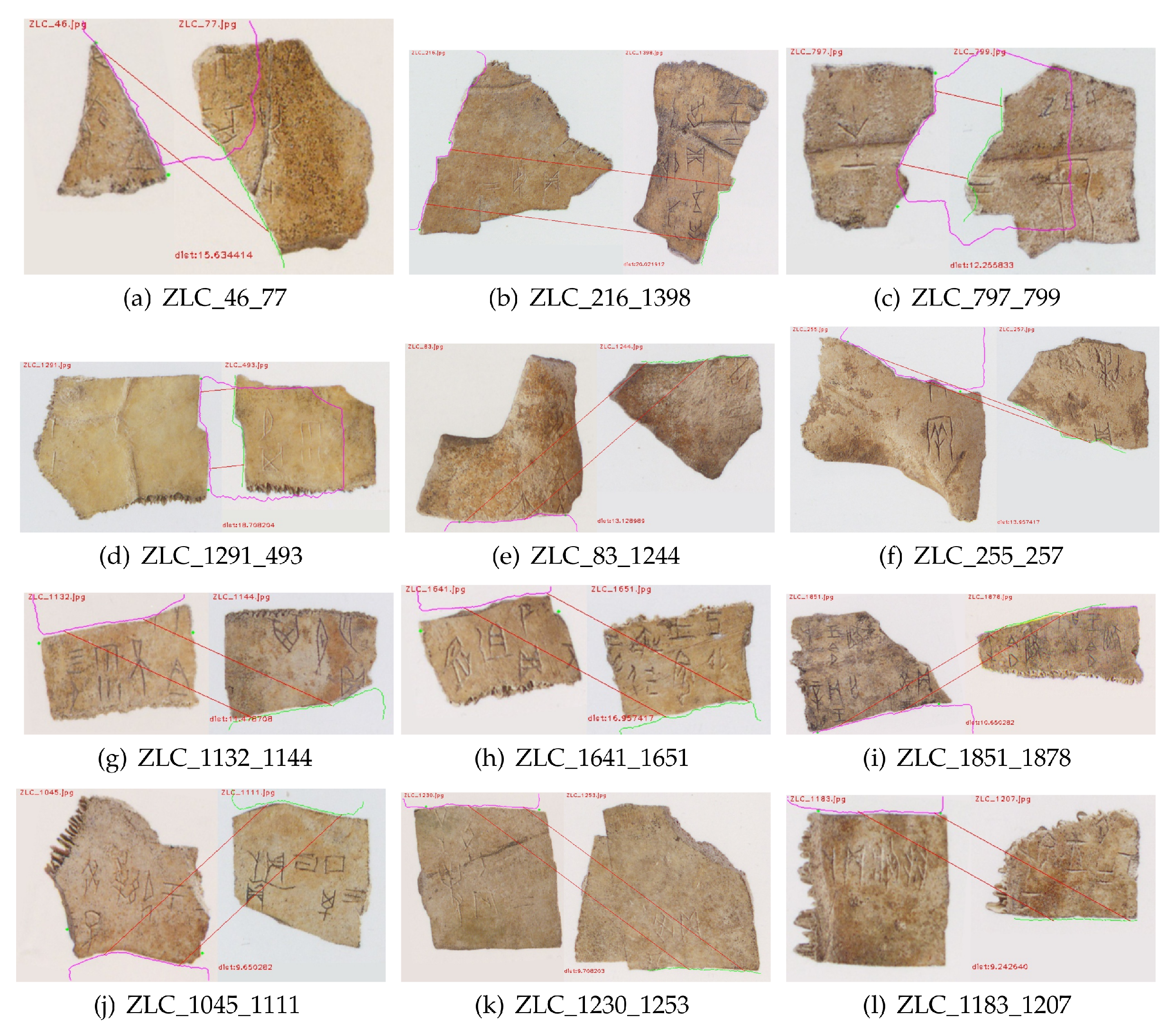
We verified the effectiveness of the EEM algorithm. It was tested on 12 pairs of rejoinable images in the ZLC image set, where 12 pixels were sampled from the original image edge segment and target image edge by the EEM algorithm, and the equidistance-increased radius of the sampling circles was set to be 10 pixels long. The EEM algorithm can accurately search the matching position of each pair of image edges, and the distances between each pair of matching sampling pixels are shown in Table 1, where the maximum distance is 20.02 pixels, the minimum distance is 9.65 pixels, the average distance of each group is 13.45 pixels and the average distance of each sampling pixels is 1.35. None of the distances exceed the threshold range.
As shown in Figure 9, there are 12 image pairs in ZLC oracle bone fragment image set, and all of them were searched by the image EEM algorithm. For each image pair, the original image’s edge segment is drawn in green, the target image’s edge is drawn in pink and the matching edge segments of the two images are between the red parallel line. The experiments showed that the image EEM algorithm given in this paper can skip the missing intermediate part in an edge segment, and thus it has good adaptability.
4.2.2. Convolution Feature Gradient Map Analysis
We verified the performance of ISN, the first order and second order gradient maps toward the convolution feature, which was extracted on the train dataset and test dataset, and the internal similarity pooling was used in the ISN model, respectively. ResNet50 was tested on the train dataset and test dataset, and, by comparing the loss of training and testing and the accuracy of training and testing, we analyzed the performance of ISP, the first order gradient map and second order gradient map toward the convolution feature. ISN was compared with ResNet50 too. The batch size was set to 100, and the model was trained in 20 epochs; it was iterated approximately 1040 times in each epoch, and approximately 20,000 times in total.
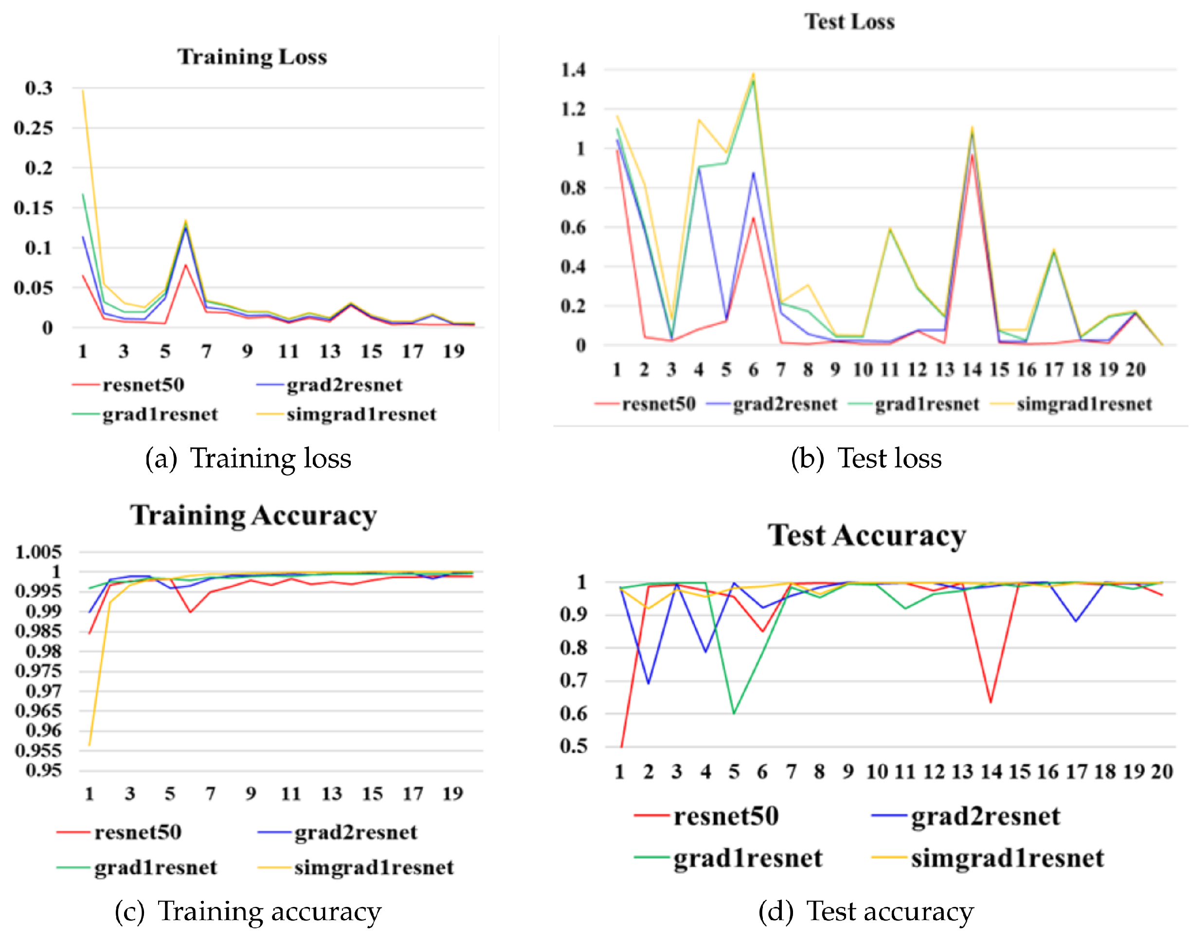
In Figure 10, the train and test loss are the normalized value, and the train and test accuracy was set to [0, 1.0]. The training loss curves of different network models are shown in Figure 10a, where the red curve denotes the loss of ResNet50, the blue curve denotes the loss of the first order convolution feature gradient map with average pooling in the second to last layer, the green curve denotes the loss of the second order convolution feature gradient map with average pooling in the second to last layer and the yellow curve denotes the loss of the ISN model. The four networks’ losses are almost the same and tend to be convergent. The test loss curves of different models are shown in Figure 10b, where the red curve indicates the test loss of ResNet50, the blue curve indicates the test loss of the first order gradient, the green curve indicates the test loss of the second order gradient feature and the yellow curve indicates the test loss of the ISN model. The test losses of the last three models are higher than that of ResNet50, but they all tend to be convergent. The phenomenon shows that adding CFGM and ISP in ResNet50 will have a lower loss and tend to be convergent after training and testing.
As shown in the training accuracy curve in Figure 10c, the accuracy of the residual network-added second order gradient is higher than that of ResNet50, and it is more stable than ResNet50. In addition, the accuracy of the residual network using the first order gradient is higher than that of the residual network using the second order gradient. At the first few epochs, the accuracy of ISN is lower than that of the other model, but at the later epochs, the ISN model’s accuracy is higher than the other models’, and it is more stable than the others’ accuracy. The test accuracy curves are shown in Figure 10d, where the test accuracy of ISN is stable above 92%, but the test accuracy of other networks fluctuates to a great extent. The training time cost by ISN is 5.79 s less than ResNet50 in each iteration; this shows that the first order gradient map of the convolution feature can improve ISN’s stability, and ISP can improve ISN’s accuracy. Furthermore, the time cost by ISN is less than the others because of a small size of input images.
4.2.3. Performance of Different Models
Table 2 shows the performance of several methods tested on the training image set. The accuracy of the ISN model is 99.98%, which is a little higher than other models; the training loss of ISN is 0.0001, which is lower than other models. The time cost by ISN is close to InceptionV3 and MobileNet, higher than AlexNet’s and lower than that of VGG19 and ResNet50. The performance on the test image set is shown in Table 3: the accuracy of the ISN model is 99.89%, and its loss is 0.0089. Among the six models, ISN has the state-of-the-art performance.
The performance of the different model is tested on the ZLC image set, and there are 1920 images and 12 pairs of rejoinable images in the set. As shown in Table 4, the ISN model has found 11 pairs of rejoinable images, and the confidence of the right judgement is 94.23%. Except MobileNet, which has the same accuracy as the ISN model, the others’ accuracies are lower than ISN.
4.3. Actual Rejoining Work
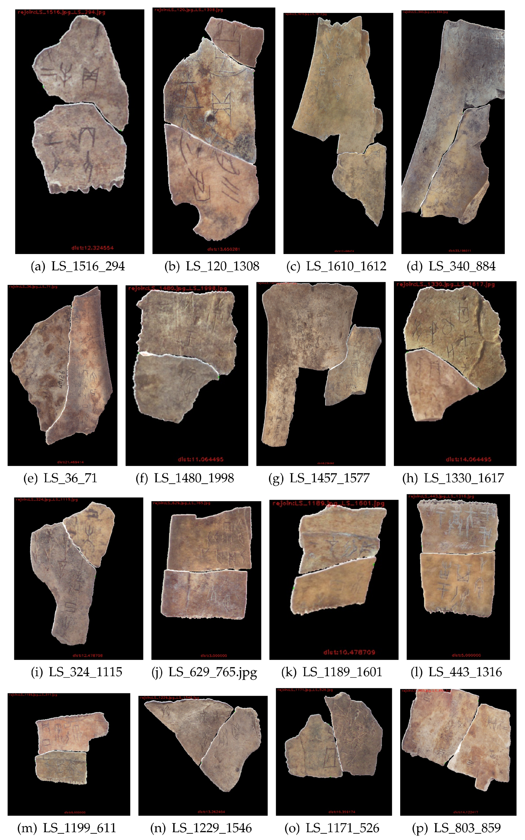
In practice, shells and bones are the two main materials of the oracle bone fragments. In the oracle bone fragments image set from Lvshun Museum, which contains 2211 images, the ISN found 16 pairs of shells and bones fragment images that can be put together into a whole image (see Figure A1). It is worth mentioning that all of these pairs were not discovered by oracle bone experts before. In addition, the oracle bone fragments are from both shells and bones in material. The experiment result demonstrates the effectiveness of the ISN for rejoining images from both shell fragments and bone fragments. Simultaneously, the result also shows that the model is more adaptable than the traditional ones, which have not found any pairs of oracle fragment images that can be joined successfully.
Our EEM algorithm found 16 pairs of matching image edge segments from the oracle bone fragment image set precisely; however, it actually labeled more than 500 image pairs that defy rejoining. Deep learning models (AlexNet, VGG19, ResNet50, InceptionV3 and MobileNet) are trained using a large amount of rejoinable and unrejoinable fragment images to improve their accuracy. The models are designed to predict similarity scores regarding the possibility of the local region images from the image pairs being rejoined together. On the image set of oracle bones fragments in Lvshun Museum, our method gives particularly high scores on the 16 pairs of successfully joined fragments; among all the high score samples that the model gives, the rejoining probability is 91.67%. However, Alexnet, VGG19 and MobileNet fail to give a correct judgement of the rejoining possibility, and InceptionV3 and ResNet50 give, respectively, five and two pairs of oracle bone image pairs that are correctly judged, which is a poor performance.
5. Conclusions
The paper introduces a new method to rejoin fragment images that has a state-of-the-art performance and can be suitable for rejoining images of shells and bones fragment, etc. At the same time, however, when the oracle bone fragments have an occlusion area that cannot be depicted in their 2D image, the EEM method will fail to find a correct matchable local edge. ISN has the ability to rejoin the texture of the fragment image, but it has a limitation in that it might make an error judgement. The future job is to improve the adaptability of the EEM algorithm and to elevate the effectiveness, accuracy and robustness of the ISN model.
Author Contributions
Z.Z.: Project administration, conceptualization, methodology, writing—original draft preparation; A.G.: formal analysis, writing—review and editing, validation; B.L.: resources, data curation, investigation. All authors have read and agreed to the published version of the manuscript.
Funding
Zhang Z. is supported by National Natural Science Foundation of China(62106007) and Department of Science and Technology of Henan Province(212102310549), Guo A. is supported by Department of Science and Technology of Henan Province(222102320189), Li B.is supported by Department of Science and Technology of Henan Province(222102210257) and Anyang City Science and Technology Development Plan (2021C01GX012). The team is supported by Ancient Characters and Chinese Civilization Inheritance and Development Project(G1806, G1807 and G2821).
Institutional Review Board Statement
Not applicable.
Informed Consent Statement
Not applicable.
Data Availability Statement
Not applicable.
Conflicts of Interest
The authors declare no conflict of interest.
Appendix A. Rejoinable Image Pairs Searched from LS Imageset
Figure A1.
Rejoinable image pairs of oracle bone fragment.

References
- Liu, Y.; Wang, T.; Wang, J. The Application of the Technique of 2D Fragments Stitching Based on Outline Feature in Rejoining Oracle Bones. In Proceedings of the International Conference on Multimedia Information Networking and Security, Nanjing, China, 4–6 November 2010; pp. 964–968. [Google Scholar]
- Alahi, A.; Ortiz, R.; Vandergheynst, P. FREAK: Fast retina keypoint. In Proceedings of the IEEE Conference on Computer Vision and Pattern Recognition, Providence, RI, USA, 16–21 June 2012; pp. 510–517. [Google Scholar]
- Kamran, H.; Zhang, K.; Li, M.; Li, X. An LCS-based 2D Fragmented Image Reassembly Algorithm. In Proceedings of the 13th International Conference on Computer Science and Education, Colombo, Sri Lanka, 8–11 August 2018; pp. 1–6. [Google Scholar]
- Zhang, Q.; Li, L.; Fang, R.; Xin, H. Reassembly of Two-Dimensional Irregular Fragments by Improved Polygon Feature Matching. In Proceedings of the IEEE 11th International Conference on Advanced Infocomm Technology, Jinan, China, 18–20 October 2019; pp. 82–85. [Google Scholar]
- Liu, W.; Wang, J.; Liu, K. Longitudinal Shredded Paper Stitching Method Based on Edge Matching. Comput. Mod. 2019, 2, 55–59. [Google Scholar]
- Zhang, M.; Chen, S.; Shu, Z.; Xin, S.; Zhao, J.; Jin, G.; Zhang, R.; Beyerer, J. Fast Algorithm for 2D Fragment Assembly Based on Partial EMD. Vis. Comput. 2016, 33, 1–12. [Google Scholar] [CrossRef]
- Paumard, M.; Picard, D.; Tabia, H. Deepzzle: Solving Visual Jigsaw Puzzles with Deep Learning and Shortest Path Optimization. Trans. Image Process. 2020, 29, 3569–3581. [Google Scholar] [CrossRef] [PubMed]
- Le, C.; Li, X. JigsawNet: Shredded Image Reassembly Using Convolutional Neural Network and Loop-Based Composition. IEEE Trans. Image Process. 2019, 28, 4000–4015. [Google Scholar] [CrossRef] [PubMed] [Green Version]
- Ngo, T.; Nguyen, C.; Nakagawa, M. A Siamese Network-based Approach for Matching Various Sizes of Excavated Wooden Fragments. In Proceedings of the 17th International Conference on Frontiers in Handwriting Recognition, Dortmund, Germany, 8–10 September 2020; pp. 307–312. [Google Scholar]
- Cécilia, O.; Beurton, M. Matching Ostraca Fragments Using A Siamese Neural Network. Pattern Recognit. Lett. 2020, 131, 336–340. [Google Scholar]
- Cécilia, O.; Beurton-Aimar, M. Using Graph Neural Networks to Reconstruct Ancient Documents. In Proceedings of the 25th International Conference on Pattern Recognition, Milan, Italy, 13 November 2020. [Google Scholar]
- Szegedy, C.; Ioffe, S.; Vanhoucke, V.; Alemi, A. Inception–V4, Inception–ResNet and the Impact of Residual Connections on Learning. In Proceedings of the 31st AAAI Conference on Artificial Intelligence, San Francisco, CA, USA, 23 February 2016; pp. 4278–4284. [Google Scholar]
- Girshick, R.; Donahue, J.; Darrell, T.; Malik, J. Rich feature hierarchies for accurate object detection and semantic segmentation. In Proceedings of the IEEE International Conference on Computer Vision, Columbus, OH, USA, 23–28 June 2014; pp. 580–587. [Google Scholar]
- He, K.; Gkioxari, G.; Dollar, P.; Girshick, R. Mask R-CNN. IEEE Trans. Pattern Anal. Mach. Intell. 2020, 42, 386–397. [Google Scholar] [CrossRef] [PubMed]
- Redmon, J.; Divvala, S.; Girshick, R.; Farhadi, A. You Only Look Once: Unified, Real-Time Object Detection. In Proceedings of the IEEE Conference on Computer Vision and Pattern Recognition, Las Vegas, NV, USA, 27–30 June 2016; pp. 779–788. [Google Scholar]
- Ruiz, L.; Gama, F.; Marques, A.G.; Ribeiro, A. Invariance-Preserving Localized Activation Functions for Graph Neural Networks. IEEE Trans. Signal Process. 2020, 68, 127–141. [Google Scholar] [CrossRef]
- He, K.; Zhang, X.; Ren, S.; Sun, J. Deep Residual Learning for Image Recognition. In Proceedings of the IEEE Conference on Computer Vision and Pattern Recognition, Las Vegas, NV, USA, 27–30 June 2016; pp. 770–778. [Google Scholar]
- He, K.; Zhang, X.; Ren, S.; Jian, S. Identity Mappings in Deep Residual Networks. In Proceedings of the 14th European Conference on Computer Vision, Amsterdam, The Netherlands, 11–14 October 2016; pp. 630–645. [Google Scholar]
- Jegou, H.; Douze, M.; Schmid, C. Product Quantization for Nearest Neighbor Search. IEEE Trans. Pattern Anal. Mach. Intell. 2011, 33, 117–128. [Google Scholar] [CrossRef] [PubMed] [Green Version]
- Zhang, Z.; Yang, D. Internal and External Similarity Aggregation Stereo Matching Algorithm. In Proceedings of the 11th International Conference on Digital Image Processing, Guangzhou, China, 10–12 May 2019; p. 1117923. [Google Scholar]
- Felzenszwalb, P.F.; Huttenlocher, D.P. Efficient Graph-Based Image Segmentation. Int. J. Comput. Vis. 2004, 59, 167–181. [Google Scholar] [CrossRef]
- Mei, X.; Sun, X.; Dong, W.; Wang, H.; Zhang, X. Segment-tree based cost aggregation for stereo matching. In Proceedings of the IEEE Computer Society Conference on Computer Vision and Pattern Recognition, Portland, OR, USA, 23–28 June 2013; pp. 313–320. [Google Scholar]
- Zhang, Z.; Wang, Y.T.; Li, B.; Guo, A.; Liu, C.L. Deep Rejoining Model for Oracle Bone Fragment Image. In Proceedings of the Asian Conference on Pattern Recognition, Jeju Island, Korea, 9–12 November 2021; Part II; pp. 3–15. [Google Scholar]
Figure 1.
A whole image rejoined from an image pair. (a) Matching edge segments of an image pair, (b) a whole image rejoined, (c) physical oracle bone fragment rejoined.
Figure 1.
A whole image rejoined from an image pair. (a) Matching edge segments of an image pair, (b) a whole image rejoined, (c) physical oracle bone fragment rejoined.

Figure 2.
Shortcut connection method, (a) two-shortcut connection, (b) dimension increase.

Figure 3.
Edge equal pixels sampling and matching, (a) edge direction and rotated edge, (b) edge equal pixel matching algorithm.
Figure 3.
Edge equal pixels sampling and matching, (a) edge direction and rotated edge, (b) edge equal pixel matching algorithm.

Figure 4.
Different arrangement mode and EEM algorithm, (a) distance between head and tail pixels, (b) edge equidistance matching.
Figure 4.
Different arrangement mode and EEM algorithm, (a) distance between head and tail pixels, (b) edge equidistance matching.

Figure 5.
Whole image rejoined based on mask, (a) mask image, (b) rejoined image.

Figure 6.
Flow chart of deep rejoining model, (a) local region image cut from a whole image, (b) rejoinable score.
Figure 6.
Flow chart of deep rejoining model, (a) local region image cut from a whole image, (b) rejoinable score.

Figure 7.
Internal similarity pooling, (a) vertical subtraction, (b) horizontal subtraction, (c) vertical gradient, (d) horizontal gradient.
Figure 7.
Internal similarity pooling, (a) vertical subtraction, (b) horizontal subtraction, (c) vertical gradient, (d) horizontal gradient.

Figure 8.
Rejoinable and unrejoinable local region images.

Figure 9.
Position of matching image edge.

Figure 10.
Performance of deep learning.


Table 1.
Distance of matching image pairs’ edge.
| Image Pair | Distance | Image Pair | Distance | Image Pair | Distance |
|---|---|---|---|---|---|
| ZLC_46 | 15.63 | ZLC_216 | 20.02 | ZLC_797 | 12.26 |
| ZLC_77 | ZLC_1398 | ZLC_799 | |||
| ZLC_1291 | 18.71 | ZLC_83 | 13.13 | ZLC_255 | 13.95 |
| ZLC_493 | ZLC_1244 | ZLC_257 | |||
| ZLC_1132 | 11.48 | ZLC_1641 | 16.96 | ZLC_1851 | 10.65 |
| ZLC_1144 | ZLC_1651 | ZLC_1878 | |||
| ZLC_1045 | 9.65 | ZLC_1230 | 9.71 | ZLC_1183 | 9.24 |
| ZLC_1111 | ZLC_1253 | ZLC_1207 |
Table 2.
Accuracy, loss and time on training dataset.
| Methods | Accuracy | Loss | Time(s/Batch) |
|---|---|---|---|
| AlexNet | 83.39% | 0.4489 | 1.41 |
| VGG19 | 83.49% | 0.4480 | 15.37 |
| ResNet50 | 99.63% | 0.0126 | 13.46 |
| InceptionV3 | 99.68% | 0.0112 | 8.12 |
| MobileNet | 99.68% | 0.0108 | 6.78 |
| ISN | 99.98% | 0.0001 | 7.67 |
Table 3.
Accuracy and loss on test dataset.
| Methods | Accuracy | Loss |
|---|---|---|
| AlexNet | 83.69% | 0.4447 |
| VGG19 | 83.38% | 0.4499 |
| ResNet50 | 95.66% | 3.2104 |
| InceptionV3 | 62.39% | 2.0513 |
| MobileNet | 90.90% | 0.1598 |
| ISN | 99.79% | 0.0089 |
Table 4.
Performance on practical rejoining job.
| Methods | Pairs | Confidence | Probability |
|---|---|---|---|
| AlexNet | 11 | 83.76% | 91.67% |
| VGG19 | 11 | 83.34% | 91.67% |
| ResNet50 | 10 | 89.07% | 83.33% |
| InceptionV3 | 8 | 66.29% | 66.66% |
| MobileNet | 11 | 96.86% | 91.67% |
| ISN | 11 | 94.23% | 91.67% |
Publisher’s Note: MDPI stays neutral with regard to jurisdictional claims in published maps and institutional affiliations. |
© 2022 by the authors. Licensee MDPI, Basel, Switzerland. This article is an open access article distributed under the terms and conditions of the Creative Commons Attribution (CC BY) license (https://creativecommons.org/licenses/by/4.0/).
Share and Cite
MDPI and ACS Style
Zhang, Z.; Guo, A.; Li, B. Internal Similarity Network for Rejoining Oracle Bone Fragment Images. Symmetry 2022, 14, 1464. https://doi.org/10.3390/sym14071464
AMA Style
Zhang Z, Guo A, Li B. Internal Similarity Network for Rejoining Oracle Bone Fragment Images. Symmetry. 2022; 14(7):1464. https://doi.org/10.3390/sym14071464
Chicago/Turabian StyleZhang, Zhan, An Guo, and Bang Li. 2022. "Internal Similarity Network for Rejoining Oracle Bone Fragment Images" Symmetry 14, no. 7: 1464. https://doi.org/10.3390/sym14071464
Note that from the first issue of 2016, this journal uses article numbers instead of page numbers. See further details here.