Topological Structure of Single-Valued Neutrosophic Hesitant Fuzzy Sets and Data Analysis for Uncertain Supply Chains

Abstract

From production to retail, the food supply chain (FSC) encompasses all stages of food production. Food is now transmitted across continents over long ranges. People depend on supply chains for basic necessities such as food, water, drinks, etc. Any disruption in these shipment pipelines poses a serious threat to human life. Supplier selection (SS) has been identified as a crucial component of FSC, which has been contemplated as a multi-criteria decision-making (MCDM) problem in many studies. The failure of some specific MCDM problems is due to failure in contemplating the relationships between alternatives under uncertain circumstances. To address such challenges, we present a contemporary method for designating green suppliers based on single-valued neutrosophic hesitant fuzzy (SVNHF) information, in which the input assessment is taken into account using single-valued neutrosophic hesitant fuzzy numbers (SVNHFNs). The foremost purpose of this analysis is to construct a topological structure on single-valued neutrosophic hesitant fuzzy sets (SVNHFSs) as well as to validate several key properties with examples. We discuss certain properties of SVNHF topology such as the SVNHF closure, SVNHF interior, SVNHF exterior, and SVNHF frontier. We also examine the conceptualization of the SVNHF dense set and SVNHF base in SVNHF topology using comprehensive examples. Eventually, to demonstrate and validate the superiority and inferiority ranking (SIR) method and choice value (CV) method in terms of their rationality and scientific basis, a real-world example of supplier selection in a food supply chain is provided. A comparative analysis is also performed to discuss the symmetry, validity and advantage of the proposed techniques.

1. Introduction

Data analysis and information aggregation techniques have been an increasing focus in various fields such as engineering, healthcare, economics, environmental concerns, and decision making. Due to uncertain information and limitations in data analysis, we cannot seek accurate and ideal evaluation in MCDM problems. To resolve such circumstances, Zadeh [1] introduced “fuzzy set theory” initially with the concept of membership function on behalf of an exact real number in $[0,1]$ to express the degree of belonging of objects under a criterion. The components of membership (MG) and non-membership (NMG) of objects were addressed by Atanassov [2] in terms of an “Intuitionistic fuzzy set (IFS)”. “Pythagorean fuzzy set” (PFS), a new method for coping with vagueness when considering membership degree ${\omega }^{\mu }$ and non-membership degree ${\omega }^{\nu }$ was proposed by Yager [3]. It can characterize uncertain information more adequately and accurately than IFSs. Although IFSs and PFSs can effectively report the attribute values in MCDM in the vast majority of instances, there are a few instances where they are deficient. In accordance with the constraints imposed by IFSs and PFSs, the attribute value cannot be represented by both IFSs and PFSs when the square sum of ${\omega }^{\mu }$ and ${\omega }^{\nu }$ degrees exceeds unity. In order to cope with this scenario, Yager [4] established the notion of the q-rung orthopair fuzzy set (q-ROFS), which can be considered a generalization of IFS and PFS. The “picture fuzzy set” (PiFS) was developed by Cuong [5], and the “spherical fuzzy set” (SFS) initiated by Mahmood et al. [6], Ashraf et al. [7], and Gündogdu and Kahraman [8]. The idea of a neutrosophic set was suggested by Smarandache [9]. Some extensions of fuzzy sets and their constraints are expressed in

Table 1. Representations of some fuzzy sets and fuzzy numbers as well as their constraints.

Fuzzy Sets	Fuzzy Numbers	Constraints
IFS [2]	$({\omega }^{\mu },{\omega }^{\nu })$	${\omega }^{\mu },{\omega }^{\nu }\in [0,1]$,       $0\le {\omega }^{\mu }+{\omega }^{\nu }\le 1$
PFS [3]	$({\omega }^{\mu },{\omega }^{\nu })$	${\omega }^{\mu },{\omega }^{\nu }\in [0,1]$,       $0\le {\left({\omega }^{\mu }\right)}^2+{\left({\omega }^{\nu }\right)}^2\le 1$
q-ROFS [4]	$({\omega }^{\mu },{\omega }^{\nu })$	${\omega }^{\mu },{\omega }^{\nu }\in [0,1]$,       $0\le {\left({\omega }^{\mu }\right)}^q+{\left({\omega }^{\nu }\right)}^q\le 1,q\ge 1$
PiFS [5]	$({\omega }^{\mu },{\omega }^I,{\omega }^{\nu })$	${\omega }^{\mu },{\omega }^I,{\omega }^{\nu }\in [0,1]$,  $0\le {\omega }^{\mu }+{\omega }^I+{\omega }^{\nu }\le 1$
SFS [6,7,8]	$({\omega }^{\mu },{\omega }^I,{\omega }^{\nu })$	${\omega }^{\mu },{\omega }^I,{\omega }^{\nu }\in [0,1]$,  $0\le {\left({\omega }^{\mu }\right)}^2+{\left({\omega }^I\right)}^2+{\left({\omega }^{\nu }\right)}^2\le 1$
NS [9]	$(T,I,F)$	$T,I,F\in ]0^{-},1^{+}[$,    $T+I+F\in [0^{-},3^{+}]$
SVNS [10]	$(T,I,F)$	$T,I,F\in [0,1]$,       $T+I+F\in [0,3]$

.

Smarandache [9] developed the “neutrosophic set” (NS) and neutrosophic logic. The neutrosophic logic is a conventional framework for determining truth, indeterminacy, and falsification. In the NS, indeterminacy is the main focus, although truth and falsity are basic components. This presumption is critical in a variety of situations, as in information fusion, which involves combining data from multiple sensors. Furthermore, because it can handle vague and imperfect information, neutrosophy appears to be preferable for modeling uncertainties, as it is rare to have complete information at one’s disposal when making decisions. The NS derives its component values from a subset of $]0^{-},1^{+}[$ that is either real or non-standard. However, in real-world engineering and scientific problems, using an NS with values from a real standard or non-standard subset of $]0^{-},1^{+}[$ is difficult. However, a single-valued neutrosophic set (SVNS) [10] derives its components $T,I,F\in [0,1]$ with $T+I+F\in [0,3]$. An SVNS [10] is a type of neutrosophic set that adds a new way to represent the undetermined, vague, imperfect, and inconsistent statistics that subsist in the the real world. It is better suited for dealing with unspecified and inconsistent data.

Molodtsov [11] proposed “soft set” (SS) theory to cope with uncertainty of parameters and their approximate elements. Hashmi et al. [12] introduced the m-polar neutrosophic set and extended it to m-polar neutrosophic topological structure with clustering analysis and healthcare. It can be difficult to regulate an element’s membership in a fixed set at times, which could be due to a misunderstanding of a collection of different values. Torra [13] suggested the notion of “hesitant fuzzy sets” (HFSs) as a generalization of FSs to better describe this situation, which permits membership degree to aid in the collection of practicable values in the closed interval [0, 1]. Experts have used HFSs to choose a variety of possible MGs to evaluate objects under suitable criteria. The theory of HFS has a diverse set of applications in a variety of disciplines, such as for computational intelligence, clustering, healthcare, and MCDM problems.

In an HFS, because of the doubts of decision makers, there is only one truth-membership hesitant function, and it is impossible to manifest this problem using only a few different values assigned by truth, indeterminacy, and falsity membership degrees. As a result, it can only represent one type of hesitancy statistics in this situation and cannot manifest three types of hesitancy statistics. To handle uncertain problems, the idea of a single-valued neutrosophic hesitant fuzzy set (SVNHFS) was introduced by Jun [14]. The truth-membership hesitancy function (TMFF), the indeterminacy-membership hesitancy function (IMHF), and the falsity-membership hesitancy function (FMHF) are three parts of the SVNHFS that can exhibit three types of hesitancy information in this state. Tanuwijaya et al. [15] proposed a novel SVNHF time series model and applied it to stock index forecasting in Indonesia and Argentina. Aggregation operators of SVNHFS were introduced by Liu et al. [16]. Wang and Li [17] proposed generalized single-valued neutrosophic hesitant fuzzy prioritized aggregation operators. The TOPSIS method for neutrosophic hesitant fuzzy multi-attribute decision making was extended by Giri et al. [18].

The CV method is a renowned and widely used MCDM basis for evaluating a set of choices using a set of criteria. Each choice is contrasted with the others by calculating a number of ratios, one per choice criterion. Every ratio is multiplied by the proportional weight of the criterion in consideration. The selection of one or more options from the set of alternatives based on the number of criteria is a fundamental task in MCDM problems.

Xu [19] proposed the SIR method, which is extension of the PROMETHEE method. The SIR method is an important MCDM approach which can grasp real data and supply the system user with six different preference structures. According to the two ranking lists, the SIR method ranks the alternatives more accurately. This method ranks alternatives using a superiority ranking list and an inferiority ranking list. The great feature of using the SIR method is that it incorporates the possessions of other MCDM techniques such as TOPSIS, SAW, and PROMETHEE. Some applications of the SIR method are given in

Table 2. Some applications of the SIR method.

Researchers	Benchmarks	Applications
Tam et al. [20]	SIR method	Concrete pump selection
Tom and Tong [21]	SIR method	Developments in the project concerning
		the location of the large-scale harbor
Liu [22]	IF SIR method	Supply chain management
Ma et al. [23]	HF SIR method	Selection of outstanding teachers from overseas
Peng and Yang [24]	PF SIR method	Investment in internet stocks
Rouhani [25]	Fuzzy SIR method	Software selection in IT field
Chen [26]	PF PROMETHEE	Bridge construction
	method with superiority
	and inferiority PFNs
Tavana et al. [27]	IFG SIR method	Solution of third-party reverse
		logistics problem
Zhao et al. [28]	SIR method with HFL	Sustainable energy technology evaluation
	prioritized value
Geetha and	PF SIR method	For investment selection of the internet
Narayanamoorthy [29]		Stock marketing companies
Jie et al. [30]	IVIF SIR method	Engineering investment selection

.

Certain novel concepts of neutrosophic sets, neutrosophic logic, and neutrosophic probability were explored in [31]. Seikh and Dutta [32] developed a matrix games model based on SVNSs. Saha and Paul [33] proposed generalized weighted exponential similarity measures for SVNSs. Alcantud et al. [34] developed generalized OWA aggregation operators and multi-agent decision making with N-soft sets. Sitara et al. [35] proposed the notion of q-rung picture fuzzy graph structures for decision analysis. Riaz et al. [36] studied recent trends in pharmaceutical logistics and supply chain management based on distance and similarity measures for bipolar fuzzy soft sets. Farid and Riaz [37] investigated the properties of Einstein interactive geometric information aggregation with q-ROFSs. Zararsiz and Riaz [38] introduced the idea of bipolar fuzzy metric spaces with applications in decision making. Riaz et al. [39] proposed topological data analysis with spherical fuzzy soft AHP-TOPSIS for an environmental mitigation system. Riaz et al. [40] proposed the idea of interval-valued linear Diophantine fuzzy Frank aggregation operators for computational intelligence and MCDM problems.

The foremost purpose of the paper is to construct the topological structure on a single-valued neutrosophic hesitant fuzzy set and to derive significant results. These results are explained with the help of examples. We define certain concepts of SVHF topology such as the interior of SVNHFS, the closure of SVNHFS, the exterior of SVNHFS, the frontier of SVNHFS, dense sets and the base of SVNHF topology. We establish an extension of the SIR technique towards SVNHF topology to deal with uncertain MCDM problems. Moreover, to demonstrate and validate the SIR method and the CV method, a practical example of supplier selection in a food supply chain is provided. A comparative analysis is also given to discuss the validity and advantage of the proposed techniques.

The organization of the rest of the paper is as follows. In Section 2, we examine some elementary conceptions such as NS, SVNS, HFS, SVNHFS, SF, and AF of SVNHFNs and operations on SVNHFSs. In Section 3, we introduce the topological structure of SVNHFSs. Section 4 introduces the SIR method, and the CV method is developed in Section 5 for SVNHF information. In Section 6, an application of the SIR method and the CV method for SVNHF information is illustrated for data analysis in uncertain supply chains. Section 5 concludes the article and discusses future directions.

2. Preliminaries

In this section, we review the notions of NS [9], SVNS [10], HFS [13], and SVNHFS [14].

Definition 1

([9]). Let $\mathcal{K}$ be a set. A NS $\mathcal{A}$ in $\mathcal{K}$ is specified by the three components defined by

$$\mathcal{A}=\left\{\langle \varsigma ,(T_{\mathcal{A}},I_{\mathcal{A}},N_{\mathcal{A}})\rangle :\varsigma \in \mathcal{K}\right\}$$

where $T_{\mathcal{A}}\left(\varsigma \right),I_{\mathcal{A}}\left(\varsigma \right),N_{\mathcal{A}}\left(\varsigma \right)\subseteq ]0^{-},1^{+}[$ such that $0^{-}\le sup{T}_{\mathcal{A}}\left(\varsigma \right)+sup{I}_{\mathcal{A}}\left(\varsigma \right)+sup$$N_{\mathcal{A}}\left(\varsigma \right)\le 3^{+}$.

Definition 2

([10]). Let $\mathcal{K}$ be a set. A SVNS $\mathcal{S}$ in $\mathcal{K}$ can be expressed as

$$\mathcal{S}=\left\{\langle \varsigma ,T_{\mathcal{S}}\left(\varsigma \right),I_{\mathcal{S}}\left(\varsigma \right),F_{\mathcal{S}}\left(\varsigma \right)\rangle \right|\varsigma \in \mathcal{K}\}$$

where the components are described by mappings $T_{\mathcal{S}},I_{\mathcal{S}},F_{\mathcal{S}}:\mathcal{S}⟶[0,1]$. The components also satisfy the condition $0\le T_{\mathcal{S}}\left(\varsigma \right)+I_{\mathcal{S}}\left(\varsigma \right)+F_{\mathcal{S}}\left(\varsigma \right)\le 3$.

Example 1.

Let $\mathcal{K}=\{{\varsigma }_1,{\varsigma }_2,{\varsigma }_3,{\varsigma }_4\}$ be a set. Then, an SVNS in $\mathcal{K}$ is of the form

$$\begin{array}{c}\hfill \mathcal{S}=\{\langle {\varsigma }_1,(0.235,0.476,0.667)\rangle ,\langle {\varsigma }_2,(0.133,0.345,0.198)\rangle ,\\ \hfill \langle {\varsigma }_3,(0.421,0.782,0.385)\rangle ,\langle {\varsigma }_4,(0.347,0.847,0.667)\rangle \}.\end{array}$$

Definition 3

([13]). Assume that $\mathcal{K}$ is a set. An HFS set can be defined as follows:

$$\mathfrak{h}=\{\langle \phi ,\check{\mathfrak{h}}\left(\phi \right)\rangle \phi \in \mathcal{K}\}$$

where $\check{\mathfrak{h}}\left(\phi \right)$ yields a finite subset of $[0,1]$. Then $\check{\mathfrak{h}}\left(\phi \right)$ denotes an HF-element that involve some values in $[0,1]$ indicating the MGs of element $\phi \in \mathcal{K}$ to the set $\mathfrak{h}$.

Example 2.

Let $\mathcal{K}=\{{\phi }_1,{\phi }_2,{\phi }_3,{\phi }_4,{\phi }_5\}$ be a set. Then, the HFS can be expressed as

$$\begin{array}{c}\hfill \mathfrak{h}=\{\langle {\phi }_1,\{0.645,0.125,0.667\}\rangle ,\langle {\phi }_2,\{0.133,0.345,0.988,0.259\}\rangle ,\\ \hfill \langle {\phi }_3,\{0.511,0.178\}\rangle ,\langle {\phi }_4,\{0.481,0.872\}\rangle ,\langle {\phi }_5,\{0.666,0.879\}\rangle \}\end{array}$$

where, $\mathfrak{h}\left({\phi }_1\right)=\{0.645,0.125,0.667\}$, $\mathfrak{h}\left({\phi }_2\right)=\{0.133,0.345,0.988,0.259\}$,

$\mathfrak{h}\left({\phi }_3\right)=\{0.511,0.178\},\mathfrak{h}\left({\phi }_4\right)=\{0.481,0.872\}$, and $\mathfrak{h}\left({\phi }_5\right)=\{0.666,0.879\}$ are HF-elements corresponding to ${\phi }_1,{\phi }_2,{\phi }_3,{\phi }_4$ and ${\phi }_5$, respectively.

Definition 4

([14]). Let $\mathcal{K}$ be a set; a SVNHFS in $\mathcal{K}$ is defined as

$${\aleph }^{{\rm Y}}=\left\{\langle {\omega }^{\mathfrak{x}},{\omega }^{\mu }\left({\omega }^{\mathfrak{x}}\right),{\omega }^I\left({\omega }^{\mathfrak{x}}\right),{\omega }^{\nu }\left({\omega }^{\mathfrak{x}}\right)\rangle |{\omega }^{\mathfrak{x}}\in \mathcal{K}\right\}$$

in which ${\omega }^{\mu }\left({\omega }^{\mathfrak{x}}\right),{\omega }^I\left({\omega }^{\mathfrak{x}}\right)$ and ${\omega }^{\nu }\left({\omega }^{\mathfrak{x}}\right)$ are three sets of some values in $[0,1]$, denoting the possible truth hesitant degrees (THD), indeterminacy hesitant degrees (IHD), and falsity hesitant degrees (FHD) of the element ${\omega }^{\mathfrak{x}}\in \mathcal{K}$ to the set ${\aleph }^{{\rm Y}}$, respectively, with the conditions $0\le {\omega }^{\mu },{\omega }^I,{\omega }^{\nu }\le 1$ and $0\le {{\omega }^{\mu }}^{+}+{{\omega }^I}^{+}+{{\omega }^{\nu }}^{+}\le 3$, where ${\omega }^{\mu }\in {\omega }^{\mu }\left({\omega }^{\mathfrak{x}}\right),{\omega }^I\in {\omega }^I\left({\omega }^{\mathfrak{x}}\right),{\omega }^{\nu }\in {\omega }^{\nu }\left({\omega }^{\mathfrak{x}}\right),{{\omega }^{\mu }}^{+}\in {{\omega }^{\mu }}^{+}\left({\omega }^{\mathfrak{x}}\right)=\underset{{\omega }^{\mu }\in {\omega }^{\mu }\left({\omega }^{\mathfrak{x}}\right)}{\cup }max\left\{{\omega }^{\mu }\right\},{{\omega }^I}^{+}\in {{\omega }^I}^{+}\left({\omega }^{\mathfrak{x}}\right)=\underset{{\omega }^I\in {\omega }^I\left({\omega }^{\mathfrak{x}}\right)}{\cup }max\left\{{\omega }^I\right\}$ and ${{\omega }^{\nu }}^{+}\in {{\omega }^{\nu }}^{+}\left({\omega }^{\mathfrak{x}}\right)=\underset{{\omega }^{\nu }\in {\omega }^{\nu }\left({\omega }^{\mathfrak{x}}\right)}{\cup }max\left\{{\omega }^{\nu }\right\}$ for ${\omega }^{\mathfrak{x}}\in \mathcal{K}$. The three-tuple $\nu \left({\omega }^{\mathfrak{x}}\right)=\{{\omega }^{\mu }\left({\omega }^{\mathfrak{x}}\right),{\omega }^I\left({\omega }^{\mathfrak{x}}\right),{\omega }^{\nu }\left({\omega }^{\mathfrak{x}}\right)\}$ is called a single-valued neutrosophic hesitant fuzzy element (SVNHFE). It can be expressed as $N=\{{\omega }^{\mu },˜{\omega }^I,˜{\omega }^{\nu }\}$.

Example 3.

Let $\mathcal{K}=\{{\omega }_1^{\mathfrak{x}},{\omega }_2^{\mathfrak{x}},{\omega }_3^{\mathfrak{x}},{\omega }_4^{\mathfrak{x}}\}$ be a set. Then, an SVNHFS ${\aleph }^{{\rm Y}}$ in $\mathcal{K}$ can be expressed as follows:

$$\begin{array}{c}\hfill {\aleph }^{{\rm Y}}=\{\langle {\omega }_1^{\mathfrak{x}},\{0.645,0.125,0.667\},\left\{0.211\right\},\{0.111,0.200\}\rangle ,\\ \hfill \langle {\omega }_2^{\mathfrak{x}},\{0.133,0.345\},\{0.988,0.259\},\{0.335,0.121\}\rangle ,\\ \hfill \langle {\omega }_3^{\mathfrak{x}},\left\{0.511\right\},\{0.124,0.654\},\{0.652,0.783,0.284\}\rangle ,\\ \hfill \langle {\omega }_4^{\mathfrak{x}},\{0.481,0.872,0.100,0.321\},\left\{0.865\right\},\left\{0.768\right\}\rangle \}\end{array}$$

Definition 5

([14]). A SVNHFS ${\aleph }^{{\rm Y}}$ is said to be null SVNHFS if ${\omega }_i^{\mu }\left({\omega }^{\mathfrak{x}}\right)=0,{\omega }_i^I\left({\omega }^{\mathfrak{x}}\right)=1$ and ${\omega }_i^{\nu }\left({\omega }^{\mathfrak{x}}\right)=1$, where i varies according to alternatives, and the null SVNHFS is denoted as ${}^0{\aleph }^{{\rm Y}}$.

A SVNHFS ${\aleph }^{{\rm Y}}$ is said to be an absolute SVNHFS if ${\omega }_i^{\mu }\left({\omega }^{\mathfrak{x}}\right)=1,{\omega }_i^I\left({\omega }^{\mathfrak{x}}\right)=0$ and ${\omega }_i^{\nu }\left({\omega }^{\mathfrak{x}}\right)=0$, where i varies according to alternatives, and the absolute SVNHFS is denoted as ${}^1{\aleph }^{{\rm Y}}$.

Definition 6

([41]). Let $N_i=〈{\omega }_i^{\mu },{\omega }_i^I,{\omega }_i^{\nu }〉(i=1,2,\dots ,n)$ be the collection of SVNHFEs. Then, the score function (SF) $\mathbb{S}\left(N_i\right)$, the accuracy function (AF) $\mathbb{A}\left(N_i\right)$, and the certainty function (CF) $\mathbb{C}\left(N_i\right)$ of $N_i(i=1,2,\dots ,n)$ can be defined as follows:

$$\begin{array}{c}\hfill \mathbb{S}\left(N_i\right)=\frac{1}{3}\left[2+\frac{1}{{\mathfrak{l}}_{{\omega }^{\mu }}}\sum _{{\omega }^{\mu }\in {\omega }^{\mu }\left({\omega }^{\mathfrak{x}}\right)}{\omega }^{\mu }-\frac{1}{{\mathfrak{l}}_{{\omega }^I}}\sum _{{\omega }^I\in {\omega }^I\left({\omega }^{\mathfrak{x}}\right)}{\omega }^I-\frac{1}{{\mathfrak{l}}_{{\omega }^{\nu }}}\sum _{{\omega }^{\nu }\in {\omega }^{\nu }\left({\omega }^{\mathfrak{x}}\right)}{\omega }^{\nu }\right]\end{array}$$

(1)

$$\begin{array}{c}\hfill \mathbb{A}\left(N_i\right)=\frac{1}{{\mathfrak{l}}_{{\omega }^{\mu }}}\sum _{{\omega }^{\mu }\in {\omega }^{\mu }\left({\omega }^{\mathfrak{x}}\right)}{\omega }^{\mu }-\frac{1}{{\mathfrak{l}}_{{\omega }^{\nu }}}\sum _{{\omega }^{\nu }\in {\omega }^{\nu }\left({\omega }^{\mathfrak{x}}\right)}{\omega }^{\nu }\end{array}$$

(2)

$$\begin{array}{c}\hfill \mathbb{C}\left(N_i\right)=\frac{1}{{\mathfrak{l}}_{{\omega }^{\mu }}}\sum _{{\omega }^{\mu }\in {\omega }^{\mu }\left({\omega }^{\mathfrak{x}}\right)}{\omega }^{\mu }\end{array}$$

(3)

SVNHFSs are used to express the method of ranking alternatives as follows, based on the concepts of SF, AF, and CF on SVNHFSs. Let $N_1$ and $N_2$ be two SVNHFEs; the ranking method is:

• If $\mathbb{S}\left(N_1\right)>\mathbb{S}\left(N_2\right)$, then $N_1$ is superior to $N_2$, designated by $N_1\succ N_2$.
• If $\mathbb{S}\left(N_1\right)=\mathbb{S}\left(N_2\right)$ and $\mathbb{A}\left(N_1\right)>\mathbb{A}\left(N_2\right)$, then $N_1$ is superior to $N_2$, designated by $N_1\succ N_2$.
• If $\mathbb{S}\left(N_1\right)=\mathbb{S}\left(N_2\right),\mathbb{A}\left(N_1\right)=\mathbb{A}\left(N_2\right)$ and $\mathbb{C}\left(N_1\right)>\mathbb{C}\left(N_2\right)$, then $N_1$ is superior to $N_2$, designated by $N_1\succ N_2$.
• If $\mathbb{S}\left(N_1\right)=\mathbb{S}\left(N_2\right),\mathbb{A}\left(N_1\right)=\mathbb{A}\left(N_2\right)$ and $\mathbb{C}\left(N_1\right)=\mathbb{C}\left(N_2\right)$, then $N_1$ is equal to $N_2$ designated by $N_1\sim N_2$.

Definition 7

([14]). Let $N_i(i=1,2,\dots ,k)$ be a cluster of SVNHFEs; the SVNHFWA operator is also an SVNHFE defined by

$SVNHFWA\left(N_1,N_2,\dots ,N_k\right)={\sum }_{i=1}^k{\theta }_i{N}_i$

$$\begin{array}{cc}\hfill =& \underset{{{\omega }^{\mu }}_1\in {\omega }_1^{\mu },\dots ,{{\omega }^{\mu }}_k\in {\omega }_k^{\mu },{{\omega }^I}_1\in {\omega }_1^I,\dots ,{{\omega }^I}_k\in {\omega }_k^I,{{\omega }^{\nu }}_1\in {\omega }_1^{\nu },\dots ,{{\omega }^{\nu }}_k\in {\omega }_k^{\nu }}{\cup }\left\{\left\{1-{\prod }_{i=1}^k{\left(1-{{\omega }^{\mu }}_i\right)}^{{\theta }_i}\right\},\right.\\ & \left.\left\{{\prod }_{i=1}^k{\left({{\omega }^I}_i\right)}^{{\theta }_i}\right\},\left\{{\prod }_{i=1}^k{\left({{\omega }^{\nu }}_i\right)}^{{\theta }_i}\right\}\right\}\end{array}$$

(4)

where $\theta ={\left({\theta }_1,{\theta }_2,\dots ,{\theta }_k\right)}^{\mu }$ is the weight vector of $N_i(i=1,2,\dots ,k)$ with ${\theta }_i>0,{\sum }_{i=1}^k{\theta }_i=1$.

The weight of each component is considered by the SVNHFWA operators, and the aggregation is also an SVNHFE.

Definition 8

([41]). Let $N_1=〈{\omega }_1^{\mu },{\omega }_1^I,{\omega }_1^{\nu }〉$ and $N_2=〈{\omega }_2^{\mu },{\omega }_2^I,{\omega }_2^{\nu }〉$ be two SVNHFEs. Then, the normalized Hamming distance between $N_1$ and $N_2$ is defined as follows:

$$\begin{array}{cc}\hfill \mathcal{D}\left(N_1,N_2\right)=& \frac{1}{3}\left(\left|\frac{1}{{\mathfrak{l}}_{{\omega }_1^{\mu }}}{\sum }_{{{\omega }^{\mu }}_1\in {\omega }_1^{\mu }\left({\omega }^{\mathfrak{x}}\right)}{{\omega }^{\mu }}_1-\frac{1}{{\mathfrak{l}}_{{\omega }_2^{\mu }}}{\sum }_{{{\omega }^{\mu }}_2\in {\omega }_2^{\mu }\left({\omega }^{\mathfrak{x}}\right)}{{\omega }^{\mu }}_2\right|+\right.\\ & \left|\frac{1}{{\mathfrak{l}}_{{\omega }_1^I}}{\sum }_{{{\omega }^I}_1\in {\omega }_1^I\left({\omega }^{\mathfrak{x}}\right)}{{\omega }^I}_1-\frac{1}{{\mathfrak{l}}_{{\omega }_2^I}}{\sum }_{{{\omega }^I}_2\in {\omega }_2^I\left({\omega }^{\mathfrak{x}}\right)}{{\omega }^I}_2\right|\\ & \left.+\left|\frac{1}{{\mathfrak{l}}_{{\omega }_1^{\nu }}}{\sum }_{{{\omega }^{\nu }}_1\in {\omega }_1^{\nu }\left({\omega }^{\mathfrak{x}}\right)}{{\omega }^{\nu }}_1-\frac{1}{{\mathfrak{l}}_{{\omega }_2^{\nu }}}\sum _{{{\omega }^{\nu }}_2\in {\omega }_2^{\nu }\left({\omega }^{\mathfrak{x}}\right)}{{\omega }^{\nu }}_2\right|\right)\end{array}$$

(5)

where ${\mathfrak{l}}_{{\omega }_k^{\mu }},{\mathfrak{l}}_{{\omega }_k^I}$ and ${\mathfrak{l}}_{{\omega }_k^{\nu }}$ are numbers of feasible membership values in $N_k$ for $k=1,2$.

Definition 9.

Let us consider two SNVHFEs $N_1=\{{\omega }_1^{\mu }\left({\omega }^{\mathfrak{x}}\right),˜{\omega }_1^I\left({\omega }^{\mathfrak{x}}\right),˜{\omega }_1^{\nu }\left({\omega }^{\mathfrak{x}}\right)\}$ and $N_2=$$\{{\omega }_2^{\mu }\left({\omega }^{\mathfrak{x}}\right),˜{\omega }_2^I\left({\omega }^{\mathfrak{x}}\right),˜{\omega }_2^{\nu }\left({\omega }^{\mathfrak{x}}\right)\}$. Some operations on SNVHFEs are defined in [14], which are the following.

• Complement: The complements of SVNHFEs $N_1$ and $N_1$ can be expressed as follows:

  $${N_1}^c=\{{\omega }_1^{\nu }\left({\omega }^{\mathfrak{x}}\right),1-{\omega }_1^I\left({\omega }^{\mathfrak{x}}\right),{\omega }_1^{\mu }\left({\omega }^{\mathfrak{x}}\right)\},$$

  $${N_2}^c=\{{\omega }_2^{\nu }\left({\omega }^{\mathfrak{x}}\right),1-{\omega }_2^I\left({\omega }^{\mathfrak{x}}\right),{\omega }_2^{\mu }\left({\omega }^{\mathfrak{x}}\right)\}.$$
• Inclusion: $N_1\subseteq N_2⟺{\omega }_1^{\mu }\left({\omega }^{\mathfrak{x}}\right)\le {\omega }_2^{\mu }\left({\omega }^{\mathfrak{x}}\right),{\omega }_1^I\left({\omega }^{\mathfrak{x}}\right)\ge {\omega }_2^I\left({\omega }^{\mathfrak{x}}\right)$ and ${\omega }_1^{\nu }\left({\omega }^{\mathfrak{x}}\right)\ge {\omega }_2^{\nu }\left({\omega }^{\mathfrak{x}}\right)$ for each ${\omega }^{\mathfrak{x}}\in {\aleph }^{{\rm Y}}$.
• The union of two SVNHFEs is defined as follows:
  $N_1\cup N_2=\{{\omega }^{\mu }\in ({\omega }_1^{\mu }\cup {\omega }_2^{\mu })|{\omega }^{\mu }\ge max({{\omega }_1^{\mu }}^{-},{{\omega }_2^{\mu }}^{-}),{\omega }^I\in ({\omega }_1^I\cap {\omega }_2^I)|{\omega }^I\le$$min({{\omega }_1^I}^{+},$${{\omega }_2^I}^{+}),{\omega }^{\nu }\in ({\omega }_1^{\nu }\cap {\omega }_2^{\nu })|{\omega }^{\nu }\le min({{\omega }_1^{\nu }}^{+},{{\omega }_2^{\nu }}^{+})\}$.
• The intersection of two SVNHFEs is defined as follows: $N_1\cap N_2=\{{\omega }^{\mu }\in ({\omega }_1^{\mu }\cap {\omega }_2^{\mu })|{\omega }^{\mu }\le$$min({{\omega }_1^{\mu }}^{+},{{\omega }_2^{\mu }}^{+}),{\omega }^I\in ({\omega }_1^I\cup {\omega }_2^I)|{\omega }^I\ge$$max({{\omega }_1^I}^{-},{{\omega }_2^I}^{-}),{\omega }^{\nu }\in ({\omega }_1^{\nu }\cup {\omega }_2^{\nu })|{\omega }^{\nu }\ge$$max({{\omega }_1^{\nu }}^{-},{{\omega }_2^{\nu }}^{-})\}$.
• $N_1\oplus N_2=\{{\omega }_1^{\mu }\oplus {\omega }_2^{\mu },{\omega }_1^I\oplus {\omega }_2^I,{\omega }_1^{\nu }\oplus {\omega }_2^{\nu }\}=\underset{{{\omega }^{\mu }}_1\in {\omega }_1^{\mu },{{\omega }^I}_1\in {\omega }_1^I,{{\omega }^{\nu }}_1\in {\omega }_1^{\nu },{{\omega }^{\mu }}_2\in {\omega }_2^{\mu },{{\omega }^I}_2\in {\omega }_2^I,{{\omega }^{\nu }}_2\in {\omega }_2^{\nu }}{\cup }\left\{\right\{{{\omega }^{\mu }}_1$
  $+{{\omega }^{\mu }}_2-{{\omega }^{\mu }}_1{{\omega }^{\mu }}_2\},\left\{{{\omega }^I}_1{{\omega }^I}_2\right\},\left\{{{\omega }^{\nu }}_1{{\omega }^{\nu }}_2\right\}\}$.
• $N_1\otimes N_2=\{{\omega }_1^{\mu }\otimes {\omega }_2^{\mu },{\omega }_1^I\otimes {\omega }_2^I,{\omega }_1^{\nu }\otimes {\omega }_2^{\nu }\}=\underset{{{\omega }^{\mu }}_1\in {\omega }_1^{\mu },{{\omega }^I}_1\in {\omega }_1^I,{{\omega }^{\nu }}_1\in {\omega }_1^{\nu },{{\omega }^{\mu }}_2\in {\omega }_2^{\mu },{{\omega }^I}_2\in {\omega }_2^I,{{\omega }^{\nu }}_2\in {\omega }_2^{\nu }}{\cup }\{\left\{{{\omega }^{\mu }}_1{{\omega }^{\mu }}_2\right\},\{{{\omega }^I}_1+{{\omega }^I}_2-{{\omega }^I}_1{{\omega }^I}_2\},$
  $\{{{\omega }^{\nu }}_1+{{\omega }^{\nu }}_2-{{\omega }^{\nu }}_1{{\omega }^{\nu }}_2\}\}$.
• $\theta N_1=\underset{{{\omega }^{\mu }}_1\in {\omega }_1^{\mu },{{\omega }^I}_1\in {\omega }_1^I,{{\omega }^{\nu }}_1\in {\omega }_1^{\nu }}{\cup }\left\{\{1-{(1-{{\omega }^{\mu }}_1)}^{\theta }\},{\left\{{{\omega }^I}_1\right)}^{\theta }\},\left\{{{{\omega }^{\nu }}_1}^{\theta }\right\}\right\},\theta >0$.
• ${N_1}^{\theta }=\underset{{{\omega }^{\mu }}_1\in {\omega }_1^{\mu },{{\omega }^I}_1\in {\omega }_1^I,{{\omega }^{\nu }}_1\in {\omega }_1^{\nu }}{\cup }\left\{\left\{{\left({{\omega }^{\mu }}_1\right)}^{\theta }\right\},\{1-{(1-{{\omega }^I}_1)}^{\theta }\},\{1-{(1-{{\omega }^{\nu }}_1)}^{\theta }\}\right\},\theta >0$.

3. SVNHF Topology

Ye [14] proposed the idea of SVNHFS as an efficient model for modeling uncertainties. Biswas et al. [41] suggested the notions of SF, AF, and CF for SVNHFEs. In this section, the notion of SVNHF topology is introduced using fundamental characteristics of SVNHFSs.

Definition 10.

Let $\mathcal{K}$ be a set and τ be the collection of SVNHFSs in $\mathcal{K}$. Then, τ is called an SVNHF topology if it satisfies following properties:

• ${}^0{\aleph }^{{\rm Y}}{,}^1{\aleph }^{{\rm Y}}\in \tau$.
• For each ${\aleph }_i^{{\rm Y}}\in \tau$, $i\in \Omega$, ${\cup }_{i\in \Omega }{\aleph }_i^{{\rm Y}}\in \tau$.
• For any ${\aleph }_1^{{\rm Y}},{\aleph }_2^{{\rm Y}}\in \tau$, ${\aleph }_1^{{\rm Y}}\cap {\aleph }_2^{{\rm Y}}\in \tau$.

Then $(\mathcal{K},\tau )$ is called SVNHF topological space.

Example 4.

Let $\mathcal{K}=\{{\omega }_1^{\mathfrak{x}},{\omega }_2^{\mathfrak{x}},{\omega }_3^{\mathfrak{x}},{\omega }_4^{\mathfrak{x}}\}$ be a set. Let us consider

$$\begin{array}{ccc}\hfill {\aleph }_1^{{\rm Y}}& =& \{\langle {\omega }_1^{\mathfrak{x}},\{0.321,0.567,0.411\},\left\{0.102\right\},\{0.536,0.844,0.689\}\rangle ,\hfill \\ & & \langle {\omega }_2^{\mathfrak{x}},\{0.213,0.469,0.328\},\{0.650,0.679\},\{0.998,0.450\}\rangle ,\hfill \\ & & \langle {\omega }_3^{\mathfrak{x}},\{0.404,0.500\},\left\{0.308\right\},\{0.792,0.670,0.666\}\rangle ,\hfill \\ & & \langle {\omega }_4^{\mathfrak{x}},\{0.210,0.410,0.589\},\{0.752,0.890,0.786\},\left\{0.450\right\}\rangle \},\hfill \\ \hfill {\aleph }_2^{{\rm Y}}& =& \{\langle {\omega }_1^{\mathfrak{x}},\{0.600,0.580,0.893\},\left\{0.100\right\},\{0.520,0.440,0.250\}\rangle ,\hfill \\ & & \langle {\omega }_2^{\mathfrak{x}},\{0.469,0.480,0.850\},\{0.210,0.650\},\{0.450,0.100\}\rangle ,\hfill \\ & & \langle {\omega }_3^{\mathfrak{x}},\{0.540,0.600\},\left\{0.300\right\},\{0.150,0.150,0.655\}\rangle ,\hfill \\ & & \langle {\omega }_4^{\mathfrak{x}},\{0.589,0.650,0.890\},\{0.095,0.350,0.750\},\left\{0.400\right\}\rangle \}\hfill \end{array}$$

any two SVNHFSs in $\mathcal{K}$.

Table 3. Union of SVNHFSs.

Union	${}^0{\mathit{\aleph }}^{\mathit{{\rm Y}}}$	${\mathit{\aleph }}_1^{\mathit{{\rm Y}}}$	${\mathit{\aleph }}_2^{\mathit{{\rm Y}}}$	${}^1{\mathit{\aleph }}^{\mathit{{\rm Y}}}$
${}^0{\aleph }^{{\rm Y}}$	${}^0{\aleph }^{{\rm Y}}$	${\aleph }_1^{{\rm Y}}$	${\aleph }_2^{{\rm Y}}$	${}^1{\aleph }^{{\rm Y}}$
${\aleph }_1^{{\rm Y}}$	${\aleph }_1^{{\rm Y}}$	${\aleph }_1^{{\rm Y}}$	${\aleph }_2^{{\rm Y}}$	${}^1{\aleph }^{{\rm Y}}$
${\aleph }_2^{{\rm Y}}$	${\aleph }_2^{{\rm Y}}$	${\aleph }_2^{{\rm Y}}$	${\aleph }_2^{{\rm Y}}$	${}^1{\aleph }^{{\rm Y}}$
${}^1{\aleph }^{{\rm Y}}$	${}^1{\aleph }^{{\rm Y}}$	${}^1{\aleph }^{{\rm Y}}$	${}^1{\aleph }^{{\rm Y}}$	$1_{\mathcal{V}}$

and 

Table 4. Intersection of SVNHFSs.

Intersection	${}^0{\mathit{\aleph }}^{\mathit{{\rm Y}}}$	${\mathit{\aleph }}_1^{\mathit{{\rm Y}}}$	${\mathit{\aleph }}_2^{\mathit{{\rm Y}}}$	${}^1{\mathit{\aleph }}^{\mathit{{\rm Y}}}$
${}^0{\aleph }^{{\rm Y}}$	${}^0{\aleph }^{{\rm Y}}$	${}^0{\aleph }^{{\rm Y}}$	${}^0{\aleph }^{{\rm Y}}$	${}^0{\aleph }^{{\rm Y}}$
${\aleph }_1^{{\rm Y}}$	${}^0{\aleph }^{{\rm Y}}$	${\aleph }_1^{{\rm Y}}$	${\aleph }_1^{{\rm Y}}$	${\aleph }_1^{{\rm Y}}$
${\aleph }_2^{{\rm Y}}$	${}^0{\aleph }^{{\rm Y}}$	${\aleph }_1^{{\rm Y}}$	${\aleph }_2^{{\rm Y}}$	${\aleph }_2^{{\rm Y}}$
${}^1{\aleph }^{{\rm Y}}$	${}^0{\aleph }^{{\rm Y}}$	${\aleph }_1^{{\rm Y}}$	${\aleph }_2^{{\rm Y}}$	${}^1{\aleph }^{{\rm Y}}$

show the union and intersection, respectively, of the SVNHFSs ${\aleph }_1^{{\rm Y}}$ and ${\aleph }_2^{{\rm Y}}$.

We see that

$${\tau }_1=\left\{{}^0{\aleph }^{{\rm Y}}{,}^1{\aleph }^{{\rm Y}}\right\}$$

$${\tau }_2=\left\{{}^0{\aleph }^{{\rm Y}},{\aleph }_1^{{\rm Y}}{,}^1{\aleph }^{{\rm Y}}\right\}$$

$${\tau }_3=\left\{{}^0{\aleph }^{{\rm Y}},{\aleph }_2^{{\rm Y}}{,}^1{\aleph }^{{\rm Y}}\right\}$$

$${\tau }_4=\left\{{}^0{\aleph }^{{\rm Y}},{\aleph }_1^{{\rm Y}},{\aleph }_2^{{\rm Y}}{,}^1{\aleph }^{{\rm Y}}\right\}$$

are SVNHF topologies on $\mathcal{K}$.

where

$$\begin{array}{ccc}\hfill {}^0{\aleph }^{{\rm Y}}& =& \{\langle {\omega }_1^{\mathfrak{x}},\{0.000,0.000,0.000\},\left\{1.000\right\},\{1.000,1.000,1.000\}\rangle ,\hfill \\ & & \langle {\omega }_2^{\mathfrak{x}},\{0.000,0.000,0.000\},\{1.000,1.000\}\},\{1.000,1.000\}\rangle ,\hfill \\ & & \langle {\omega }_3^{\mathfrak{x}},\{0.000,0.000\},\left\{1.000\right\},\{1.000,1.000,1.000\}\rangle ,\hfill \\ & & \langle {\omega }_4^{\mathfrak{x}},\{0.000,0.000,0.000\},\{1.000,1.000,1.000\},\left\{1.000\right\}\rangle \}\hfill \end{array}$$

is a null SVNHFS in $\mathcal{K}$.

$$\begin{array}{ccc}\hfill {}^1{\aleph }^{{\rm Y}}& =& \{\langle {\omega }_1^{\mathfrak{x}},\{1.000,1.000,1.000\},\left\{0.000\right\},\{0.000,0.000,0.000\}\rangle ,\hfill \\ & & \langle {\omega }_2^{\mathfrak{x}},\{1.000,1.000,1.000\},\{0.000,0.000\}\},\{0.000,0.000\}\rangle ,\hfill \\ & & \langle {\omega }_3^{\mathfrak{x}},\{1.000,1.000\},\left\{0.000\right\},\{0.000,0.000,0.000\}\rangle ,\hfill \\ & & \langle {\omega }_4^{\mathfrak{x}},\{1.000,1.000,1.000\},\{0.000,0.000,0.000\},\left\{0.000\right\}\rangle \}\hfill \end{array}$$

is an absolute SVNHFS in $\mathcal{K}$.

Definition 11.

If $(\mathcal{K},\tau )$ is an SVNHF topological space over $\mathcal{K}$, then the members of SVNHF topology τ are called SVNHF open sets. That is, if ${\aleph }^{{\rm Y}}\in \tau$, then ${\aleph }^{{\rm Y}}$ is called an SVNHF open set.

Theorem 1.

If $(\mathcal{K},\tau )$ is any SVNHF topological space, then

• ${}^0{\aleph }^{{\rm Y}}$ and ${}^1{\aleph }^{{\rm Y}}$ are SVNHF open sets;
• $\underset{\omega \in \Omega }{\cup }{\aleph }_{\omega }^{{\rm Y}}$ is an SVNHF open set, where each ${\aleph }_{\omega }^{{\rm Y}}$ is an SVNHF open set;
• ${\cap }_{i=1}^n{\aleph }_i^{{\rm Y}}$ is an SVNHF open set, where each ${\aleph }_i^{{\rm Y}}$ is an SVNHF open set.

Proof .

• From the definition of SVNHF topology τ, ${}^0{\aleph }^{{\rm Y}}$, ${}^1{\aleph }^{{\rm Y}}\in \tau$. Hence, ${}^0{\aleph }^{{\rm Y}}$ and ${}^1{\aleph }^{{\rm Y}}$ are SVNHF open sets.
• Let $\left\{{\left({\aleph }_{\omega }^{{\rm Y}}\right)}_{\omega \in \Omega }\right\}$ be SVNHF open sets. Then, ${\aleph }_{\omega }^{{\rm Y}}\in \tau$. By the definition of τ

  $$\underset{\omega \in \Omega }{\cup }{\aleph }_{\omega }^{{\rm Y}}\in \tau$$
  Hence, $\underset{\omega \in \Omega }{\cup }{\aleph }_{\omega }^{{\rm Y}}$ is SVNHF open set.
• Let ${\aleph }_1^{{\rm Y}},{\aleph }_2^{{\rm Y}},\cdots ,{\aleph }_n^{{\rm Y}}$ be SVNHF open sets. Then, by the definition of τ,

  $${\cap }_{i=1}^n{\aleph }_i^{{\rm Y}}\in \tau$$
  Hence, ${\cap }_{i=1}^n{\aleph }_i^{{\rm Y}}$ is an SVNHF open set.

   □

Definition 12.

Let $(\mathcal{K},\tau )$ be an SVNHF topological space over $\mathcal{K}$. If the complement of an SVNHFS is SVNHF open, then it is called an SVNHF closed set in $\mathcal{K}$. That is, ${\aleph }^{{\rm Y}}$ is called an SVNHF closed set if, and only if, ${\left({\aleph }^{{\rm Y}}\right)}^c\in \tau$.

Theorem 2.

Assume that $(\mathcal{K},\tau )$ is an SVNHF topological space. Then,

• ${}^0{\aleph }^{{\rm Y}}{,}^1{\aleph }^{{\rm Y}}$ are SVNHF closed sets over $\mathcal{K}$;
• ${\displaystyle {(\cap {\aleph }_{\omega }^{{\rm Y}})}_{\omega \in \Omega }}$ is an SVNHF closed set over $\mathcal{K}$, where each ${\aleph }_{\omega }^{{\rm Y}}$ is an SVNHF closed set;
• $(\cup {\aleph }_i^{{\rm Y}})$ is an SVNHF closed set over $\mathcal{K}$, for any SVNHF closed sets ${\aleph }_1^{{\rm Y}}$ and ${\aleph }_2^{{\rm Y}}$.

Proof .

The proof is obvious.    □

Definition 13.

Let $(\mathcal{K},{\tau }_1)$ and $(\mathcal{K},{\tau }_2)$ be two SVNHF topological spaces over same set $\mathcal{K}$. If ${\tau }_1\subseteq {\tau }_2$, then ${\tau }_1$ is said to be SVNHF coarser or SVNHF weaker than ${\tau }_2$, and ${\tau }_2$ is said to be SVNHF finer or SVNHF stronger than ${\tau }_1$.

If ${\tau }_1⊈{\tau }_2$ or ${\tau }_2⊈{\tau }_1$, then these SVNHF topologies are not comparable.

Example 5.

From Example 4, let us consider ${\tau }_2={\{}^0{\aleph }^{{\rm Y}},{\aleph }_1^{{\rm Y}}{,}^1{\aleph }^{{\rm Y}}\}$ and ${\tau }_4={\{}^0{\aleph }^{{\rm Y}},{\aleph }_1^{{\rm Y}}{\aleph }_2^{{\rm Y}}{,}^1{\aleph }^{{\rm Y}}\}$, two SVNHF topologies on $\mathcal{K}$. It is comprehensible that ${\tau }_2\subseteq {\tau }_4$. Thus, ${\tau }_2$ is SVNHF coarser than ${\tau }_4$ and ${\tau }_4$ is SVNHF finer than ${\tau }_2$.

Definition 14.

Assume a universal set $\mathcal{K}$, and the assemblage of all SVNHFSs τ is defined over $\mathcal{K}$. Then, τ is an SVNHF discrete topology on $\mathcal{K}$, and $(\mathcal{K},\tau )$ is known as SVNHF discrete topological space over $\mathcal{K}$.

Definition 15.

Suppose that $\mathcal{K}$ is a universal set and $\tau ={\{}^0{\aleph }^{{\rm Y}}{,}^1{\aleph }^{{\rm Y}}\}$. Then, τ is an SVNHF non-discrete topology on $\mathcal{K}$ and $(\mathcal{K},\tau )$ is an SVNHF non-discrete topological space over $\mathcal{K}$.

Theorem 3.

Suppose that $(\mathcal{K},{\tau }_1)$ and $(\mathcal{K},{\tau }_2)$ are two SVNHF topological spaces over identical universes of discourse $\mathcal{K}$; then, $(\mathcal{K},{\tau }_1\cap {\tau }_2)$ is an SVNHF topological space over $\mathcal{K}$.

Proof .

The proof is obvious.    □

Definition 16.

Let us consider an SVNHF topological space $(\mathcal{K},\tau )$. For any SVNHFS ${\aleph }^{{\rm Y}}$ of $\mathcal{K}$, the SVNHF interior ${\left({\aleph }^{{\rm Y}}\right)}^{\circ }$ is interpreted as the union of all SVNHF open subsets of ${\aleph }^{{\rm Y}}$. ${\left({\aleph }^{{\rm Y}}\right)}^{\circ }$ is the largest SVNHF open set contained in ${\aleph }^{{\rm Y}}$.

Example 6.

From Example 4, we see that $\tau ={\{}^0{\aleph }^{{\rm Y}},{\aleph }_1^{{\rm Y}},{\aleph }_2^{{\rm Y}}{,}^1{\aleph }^{{\rm Y}}\}$ is an SVNHF topology on $\mathcal{K}$.Consider an SVNHFS defined on $\mathcal{K}=\{{\omega }_1^{\mathfrak{x}},{\omega }_2^{\mathfrak{x}},{\omega }_3^{\mathfrak{x}},{\omega }_4^{\mathfrak{x}}\}$

$$\begin{array}{ccc}\hfill {\aleph }^{{\rm Y}}& =& \left\{\right(\langle {\omega }_1^{\mathfrak{x}},\{0.400,0.575,0.589\},\left\{0.101\right\},\{0.530,0.540,0.570\}\rangle ,\hfill \\ & & \langle {\omega }_2^{\mathfrak{x}},\{0.369,0.470,0.638\},\{0.400,0.660\},\{0.700,0.200\}\rangle ,\hfill \\ & & \langle {\omega }_3^{\mathfrak{x}},\{0.500,0.550\},\left\{0.305\right\},\{0.400,0.380,0.660\}\rangle \hfill \\ & & \langle {\omega }_4^{\mathfrak{x}},\{0.330,0.500,0.700\},\{0.400,0.611,0.770\},\left\{0.440\right\}\rangle \}\hfill \end{array}$$

Then, ${\left({\aleph }^{{\rm Y}}\right)}^{\circ }={}^0{\aleph }^{{\rm Y}}\cup {\aleph }_1^{{\rm Y}}={\aleph }_1^{{\rm Y}}$.

Theorem 4.

Assume that $(\mathcal{K},\tau )$ is an SVNHF topological space over $\mathcal{K}$, ${\aleph }_1^{{\rm Y}}$ and ${\aleph }_2^{{\rm Y}}$ are SVNHFSs over $\mathcal{K}$. Then,

• ${\left({\aleph }_1^{{\rm Y}}\right)}^{\circ }\subseteq {\aleph }_1^{{\rm Y}}$
• ${\left({\aleph }_1^{{\rm Y}}\right)}^{\circ }={\left({\left({\aleph }_1^{{\rm Y}}\right)}^{\circ }\right)}^{\circ }$
• ${\aleph }_1^{{\rm Y}}$ is an SVNHF open set $⟺{\left({\aleph }_1^{{\rm Y}}\right)}^{\circ }={\aleph }_1^{{\rm Y}}$
• ${\left({\aleph }_1^{{\rm Y}}\right)}^{\circ }\subseteq {\left({\aleph }_2^{{\rm Y}}\right)}^{\circ }$ if ${\aleph }_1^{{\rm Y}}\subseteq {\aleph }_2^{{\rm Y}}$
• ${\left({\aleph }_1^{{\rm Y}}\right)}^{\circ }\cap {\left({\aleph }_2^{{\rm Y}}\right)}^{\circ }={\left({\aleph }_1^{{\rm Y}}\cap {\aleph }_2^{{\rm Y}}\right)}^{\circ }$
• ${\left({\aleph }_1^{{\rm Y}}\right)}^{\circ }\cup {\left({\aleph }_2^{{\rm Y}}\right)}^{\circ }\subseteq {\left({\aleph }_1^{{\rm Y}}\cup {\aleph }_2^{{\rm Y}}\right)}^{\circ }$

Proof .

• This is obvious from the definition of the SVNHF interior.
• Since ${\left({\aleph }_1^{{\rm Y}}\right)}^{\circ }$ is an SVNHF open set and it is also the biggest SVNHF open subset of itself, ${\left({\aleph }_1^{{\rm Y}}\right)}^{\circ }={\left({\left({\aleph }_1^{{\rm Y}}\right)}^{\circ }\right)}^{\circ }$.
• If ${\aleph }_1^{{\rm Y}}$ is an SVNHF open subset, then ${\aleph }_1^{{\rm Y}}$ will be an SVNHF interior of itself since it is the largest SVNHF open subset. Conversely, if ${\left({\aleph }_1^{{\rm Y}}\right)}^{\circ }={\aleph }_1^{{\rm Y}}$, then ${\aleph }_1^{{\rm Y}}$ is an SVNHF open set because ${\left({\aleph }_1^{{\rm Y}}\right)}^{\circ }$ is SVNHF open.
• Since ${\aleph }_1^{{\rm Y}}\subseteq {\aleph }_2^{{\rm Y}}$, from part $\left(1\right)$, ${\left({\aleph }_1^{{\rm Y}}\right)}^{\circ }\subseteq {\aleph }_1^{{\rm Y}}\subseteq {\aleph }_2^{{\rm Y}}$. ${\left({\aleph }_1^{{\rm Y}}\right)}^{\circ }$ is an SVNHF open subset of ${\aleph }_2^{{\rm Y}}$ and so, by the definition of ${\left({\aleph }_2^{{\rm Y}}\right)}^{\circ }$, we have ${\left({\aleph }_1^{{\rm Y}}\right)}^{\circ }\subseteq {\left({\aleph }_2^{{\rm Y}}\right)}^{\circ }$
• From part $\left(4\right)$,
  ${\aleph }_1^{{\rm Y}}\cap {\aleph }_2^{{\rm Y}}\subseteq {\aleph }_1^{{\rm Y}}$ and ${\aleph }_1^{{\rm Y}}\cap {\aleph }_2^{{\rm Y}}\subseteq {\aleph }_2^{{\rm Y}}$
  $⟹{({\aleph }_1^{{\rm Y}}\cap {\aleph }_2^{{\rm Y}})}^{\circ }\subseteq {\left({\aleph }_1^{{\rm Y}}\right)}^{\circ }$ and ${({\aleph }_1^{{\rm Y}}\cap {\aleph }_2^{{\rm Y}})}^{\circ }\subseteq {\left({\aleph }_2^{{\rm Y}}\right)}^{\circ }$
  so that
  ${({\aleph }_1^{{\rm Y}}\cap {\aleph }_2^{{\rm Y}})}^{\circ }\subseteq {\left({\aleph }_1^{{\rm Y}}\right)}^{\circ }\cap {\left({\aleph }_2^{{\rm Y}}\right)}^{\circ }$
  Furthermore, since ${\left({\aleph }_1^{{\rm Y}}\right)}^{\circ }\subseteq {\aleph }_1^{{\rm Y}},{\left({\aleph }_2^{{\rm Y}}\right)}^{\circ }\subseteq {\aleph }_2^{{\rm Y}},{\left({\aleph }_1^{{\rm Y}}\right)}^{\circ }\cap {\left({\aleph }_2^{{\rm Y}}\right)}^{\circ }\subseteq {\aleph }_1^{{\rm Y}}\cap {\aleph }_2^{{\rm Y}}$, so that ${\left({\aleph }_1^{{\rm Y}}\right)}^{\circ }\cap {\left({\aleph }_2^{{\rm Y}}\right)}^{\circ }$ is an SVNHF open subset of ${\aleph }_1^{{\rm Y}}\cap {\aleph }_2^{{\rm Y}}$. Hence,
  ${\left({\aleph }_1^{{\rm Y}}\right)}^{\circ }\cap {\left({\aleph }_2^{{\rm Y}}\right)}^{\circ }\subseteq {\left({\aleph }_1^{{\rm Y}}\cap {\aleph }_2^{{\rm Y}}\right)}^{\circ }$
  Thus,
  ${\left({\aleph }_1^{{\rm Y}}\cap {\aleph }_2^{{\rm Y}}\right)}^{\circ }={\left({\aleph }_1^{{\rm Y}}\right)}^{\circ }\cap {\left({\aleph }_2^{{\rm Y}}\right)}^{\circ }$.
• From ${\aleph }_1^{{\rm Y}}\subseteq {\aleph }_1^{{\rm Y}}\cup {\aleph }_2^{{\rm Y}},{\aleph }_2^{{\rm Y}}\subseteq {\aleph }_1^{{\rm Y}}\cup {\aleph }_2^{{\rm Y}}$
  we have
  ${\left({\aleph }_1^{{\rm Y}}\right)}^{\circ }\subseteq {({\aleph }_1^{{\rm Y}}\cup {\aleph }_2^{{\rm Y}})}^{\circ },{\left({\aleph }_2^{{\rm Y}}\right)}^{\circ }\subseteq {({\aleph }_1^{{\rm Y}}\cup {\aleph }_2^{{\rm Y}})}^{\circ }$
  so that, because ${\left({\aleph }_1^{{\rm Y}}\right)}^{\circ }\cup {\left({\aleph }_2^{{\rm Y}}\right)}^{\circ }$ is SVNHF open,
  ${\left({\aleph }_1^{{\rm Y}}\right)}^{\circ }\cup {\left({\aleph }_2^{{\rm Y}}\right)}^{\circ }\subseteq {({\aleph }_1^{{\rm Y}}\cup {\aleph }_2^{{\rm Y}})}^{\circ }$.

   □

Definition 17.

Let us consider an SVNHF topological space $(\mathcal{K},\tau )$. For any SVNHFS ${\aleph }^{{\rm Y}}$ of $\mathcal{K}$, the SVNHF closure $\overline{{\aleph }^{{\rm Y}}}$ is the intersection of all SVNHF closed super sets of ${\aleph }^{{\rm Y}}$.

Example 7.

Consider an SVNHF topology $\tau ={\{}^0{\aleph }^{{\rm Y}},{\aleph }_1^{{\rm Y}},{\aleph }_2^{{\rm Y}}{,}^1{\aleph }^{{\rm Y}}\}$ on $\mathcal{K}$ defined in Example 4 and an SVNHFS defined in Example 6 For SVNHF closure, we have to find the complements of ${\aleph }_1^{{\rm Y}},{\aleph }_2^{{\rm Y}}{,}^0{\aleph }^{{\rm Y}}$ and ${}^1{\aleph }^{{\rm Y}}$.

$$\begin{array}{ccc}\hfill {\left({\aleph }_1^{{\rm Y}}\right)}^c& =& \left\{\right(\langle {\omega }_1^{\mathfrak{x}},\{0.536,0.844,0.689\},\left\{0.898\right\},\{0.321,0.567,0.411\}\rangle ,\hfill \\ & & \langle {\omega }_2^{\mathfrak{x}},\{0.998,0.450\},\{0.350,0.321\},\{0.213,0.469,0.328\}\rangle ,\hfill \\ & & \langle {\omega }_3^{\mathfrak{x}},\{0.792,0.670,0.666\},\left\{0.692\right\},\{0.404,0.500\}\rangle \hfill \\ & & \langle {\omega }_4^{\mathfrak{x}},\left\{0.450\right\},\{0.248,0.110,0.214\},\{0.210,0.410,0.589\}\rangle \}\hfill \\ \hfill {\left({\aleph }_2^{{\rm Y}}\right)}^c& =& \{\langle {\omega }_1^{\mathfrak{x}},\{0.520,0.440,0.250\},\left\{0.900\right\},\{0.600,0.580,0.893\}\rangle ,\hfill \\ & & \langle {\omega }_2^{\mathfrak{x}},\{0.450,0.100\},\{0.790,0.350\},\{0.469,0.480,0.850\}\rangle ,\hfill \\ & & \langle {\omega }_3^{\mathfrak{x}},\{0.150,0.150,0.655\},\left\{0.700\right\},\{0.540,0.600\}\rangle \hfill \\ & & \langle {\omega }_4^{\mathfrak{x}},\left\{0.400\right\},\{0.905,0.650,0.250\},\{0.589,0.650,0.890\}\rangle \}\hfill \\ \hfill {\left({}^0{\aleph }^{{\rm Y}}\right)}^c& =& \{\langle {\omega }_1^{\mathfrak{x}},\{1.000,1.000,1.000\},\left\{0.000\right\},\{0.000,0.000,0.000\}\rangle ,\hfill \\ & & \langle {\omega }_2^{\mathfrak{x}},\{1.000,1.000,1.000\},\{0.000,0.000\}\},\{0.000,0.000\}\rangle ,\hfill \\ & & \langle {\omega }_3^{\mathfrak{x}},\{1.000,1.000\},\left\{0.000\right\},\{0.000,0.000,0.000\}\rangle ,\hfill \\ & & \langle {\omega }_4^{\mathfrak{x}},\{1.000,1.000,1.000\},\{0.000,0.000,0.000\},\left\{0.000\right\}\}\hfill \\ \hfill {\left({}^1{\aleph }^{{\rm Y}}\right)}^c& =& \{\langle {\omega }_1^{\mathfrak{x}},\{0.000,0.000,0.000\},\left\{1.000\right\},\{1.000,1.000,1.000\}\rangle ,\hfill \\ & & \langle {\omega }_2^{\mathfrak{x}},\{0.000,0.000,0.000\},\{1.000,1.000\}\},\{1.000,1.000\}\rangle ,\hfill \\ & & \langle {\omega }_3^{\mathfrak{x}},\{0.000,0.000\},\left\{1.000\right\},\{1.000,1.000,1.000\}\rangle ,\hfill \\ & & \langle {\omega }_4^{\mathfrak{x}},\{0.000,0.000,0.000\},\{1.000,1.000,1.000\},\left\{1.000\right\}\}\hfill \end{array}$$

Then, $\overline{{\aleph }^{{\rm Y}}}={\left({}^0{\aleph }^{{\rm Y}}\right)}^c={}^1{\aleph }^{{\rm Y}}$.

Theorem 5.

Suppose that $\mathcal{K}$ is a universal set, that $(\mathcal{K},\tau )$ is an SVNHF topological space over $\mathcal{K}$, and that ${\aleph }_1^{{\rm Y}}$ and ${\aleph }_2^{{\rm Y}}$ are SVNHFSs over $\mathcal{K}$. Then,

• $\overline{{}^0{\aleph }^{{\rm Y}}}{=}^0{\aleph }^{{\rm Y}}$ and $\overline{{}^1{\aleph }^{{\rm Y}}}={}^1{\aleph }^{{\rm Y}}$
• ${\aleph }_1^{{\rm Y}}\subseteq \overline{{\aleph }_1^{{\rm Y}}}$
• ${\aleph }_1^{{\rm Y}}$ is an SVNHF closed set $⟺{\aleph }_1^{{\rm Y}}=\overline{{\aleph }_1^{{\rm Y}}}$
• $\overline{\overline{{\aleph }_1^{{\rm Y}}}}=\overline{{\aleph }_1^{{\rm Y}}}$
• $\overline{{\aleph }_1^{{\rm Y}}}\subseteq \overline{{\aleph }_2^{{\rm Y}}}$ if ${\aleph }_1^{{\rm Y}}\subseteq {\aleph }_2^{{\rm Y}}$
• $\overline{{\aleph }_1^{{\rm Y}}}\cup \overline{{\aleph }_2^{{\rm Y}}}=\overline{{\aleph }_1^{{\rm Y}}\cup {\aleph }_2^{{\rm Y}}}$
• $\overline{{\aleph }_1^{{\rm Y}}\cap {\aleph }_2^{{\rm Y}}}\subseteq \overline{{\aleph }_1^{{\rm Y}}}\cap \overline{{\aleph }_2^{{\rm Y}}}$

Proof .

• By definition, ${}^0{\aleph }^{{\rm Y}}\subseteq \overline{{}^0{\aleph }^{{\rm Y}}}$. Since ${}^0{\aleph }^{{\rm Y}}$ is an SVNHF closed superset of itself, $\overline{{}^0{\aleph }^{{\rm Y}}}\subseteq {}^0{\aleph }^{{\rm Y}}$. Thus, $\overline{{}^0{\aleph }^{{\rm Y}}}={}^0{\aleph }^{{\rm Y}}$. Similarly, $\overline{{}^1{\aleph }^{{\rm Y}}}={}^1{\aleph }^{{\rm Y}}$.
• By definition, ${\aleph }_1^{{\rm Y}}\subseteq \overline{{\aleph }_1^{{\rm Y}}}$, because $\overline{{\aleph }_1^{{\rm Y}}}$ is the intersection of all SVNHF closed supersets of ${\aleph }_1^{{\rm Y}}$.
• The proof is obvious.
• Since $\overline{{\aleph }_1^{{\rm Y}}}$ is an SVNHF closed set, by $\left(3\right)$ we have $\overline{\overline{{\aleph }_1^{{\rm Y}}}}=\overline{{\aleph }_1^{{\rm Y}}}$.
• Suppose ${\aleph }_1^{{\rm Y}}\subseteq {\aleph }_2^{{\rm Y}}$ as ${\aleph }_2^{{\rm Y}}\subseteq \overline{{\aleph }_2^{{\rm Y}}}$. Therefore, ${\aleph }_1^{{\rm Y}}\subseteq \overline{{\aleph }_2^{{\rm Y}}}$. This means that $\overline{{\aleph }_2^{{\rm Y}}}$ is an SVNHF closed superset of ${\aleph }_1^{{\rm Y}}$. Thus, $\overline{{\aleph }_1^{{\rm Y}}}\subseteq \overline{{\aleph }_2^{{\rm Y}}}$.
• As we know that ${\aleph }_1^{{\rm Y}}\subseteq {\aleph }_1^{{\rm Y}}\cup {\aleph }_2^{{\rm Y}}$ and ${\aleph }_2^{{\rm Y}}\subseteq {\aleph }_1^{{\rm Y}}\cup {\aleph }_2^{{\rm Y}}$, by using part $\left(5\right)$, $\overline{{\aleph }_1^{{\rm Y}}}\subseteq \overline{{\aleph }_1^{{\rm Y}}\cup {\aleph }_2^{{\rm Y}}}$ and $\overline{{\aleph }_2^{{\rm Y}}}\subseteq \overline{{\aleph }_1^{{\rm Y}}\cup {\aleph }_2^{{\rm Y}}}$.
  $⟹\overline{{\aleph }_1^{{\rm Y}}}\cup \overline{{\aleph }_2^{{\rm Y}}}\subseteq \overline{{\aleph }_1^{{\rm Y}}\cup {\aleph }_2^{{\rm Y}}}$.
  Conversely, suppose that ${\aleph }_1^{{\rm Y}}\subseteq \overline{{\aleph }_1^{{\rm Y}}}$ and ${\aleph }_2^{{\rm Y}}\subseteq \overline{{\aleph }_2^{{\rm Y}}}$.
  Thus, ${\aleph }_1^{{\rm Y}}\cup {\aleph }_2^{{\rm Y}}\subseteq \overline{{\aleph }_1^{{\rm Y}}\cup {\aleph }_2^{{\rm Y}}}$.
  Since $\overline{{\aleph }_1^{{\rm Y}}}\cup \overline{{\aleph }_2^{{\rm Y}}}$ is s SVNHF closed superset of ${\aleph }_1^{{\rm Y}}\cup {\aleph }_2^{{\rm Y}}$.Therefore, $\overline{{\aleph }_1^{{\rm Y}}\cup {\aleph }_2^{{\rm Y}}}\subseteq \overline{{\aleph }_1^{{\rm Y}}}\cup \overline{{\aleph }_2^{{\rm Y}}}$.
  Thus, $\overline{{\aleph }_1^{{\rm Y}}}\cup \overline{{\aleph }_2^{{\rm Y}}}=\overline{{\aleph }_1^{{\rm Y}}\cup {\aleph }_2^{{\rm Y}}}$.
• If ${\aleph }_1^{{\rm Y}}\cap {\aleph }_2^{{\rm Y}}\subseteq {\aleph }_1^{{\rm Y}}$ and ${\aleph }_1^{{\rm Y}}\cap {\aleph }_2^{{\rm Y}}\subseteq {\aleph }_2^{{\rm Y}}$, then $\overline{{\aleph }_1^{{\rm Y}}\cap {\aleph }_2^{{\rm Y}}}\subseteq \overline{{\aleph }_1^{{\rm Y}}}$ and $\overline{{\aleph }_1^{{\rm Y}}\cap {\aleph }_2^{{\rm Y}}}\subseteq \overline{{\aleph }_2^{{\rm Y}}}$. Thus, $\overline{{\aleph }_1^{{\rm Y}}\cap {\aleph }_2^{{\rm Y}}}\subseteq \overline{{\aleph }_1^{{\rm Y}}}\cap \overline{{\aleph }_2^{{\rm Y}}}$.

   □

Definition 18.

Let us consider an SVNHF topological space $(\mathcal{K},\tau )$. For any SVNHFS ${\aleph }^{{\rm Y}}$ of $\mathcal{K}$, the SVNHF exterior Ext$\left({\aleph }^{{\rm Y}}\right)$ is interpreted as the interior of the complement of SVNHFS ${\aleph }^{{\rm Y}}$.

Example 8.

From Example 4, consider an SVNHF topology $\tau ={\{}^0{\aleph }^{{\rm Y}},{\aleph }_1^{{\rm Y}},{\aleph }_2^{{\rm Y}}{,}^1{\aleph }^{{\rm Y}}\}$ on $\mathcal{K}$ and an SVNHFS defined in Example 6. For SVNHF exterior, we have to find the complement of ${\aleph }^{{\rm Y}}$.

$$\begin{array}{ccc}\hfill {\left({\aleph }^{{\rm Y}}\right)}^c& =& \left\{\right(\langle {\omega }_1^{\mathfrak{x}},\{0.530,0.540,0.570\},\left\{0.899\right\},\{0.400,0.575,0.589\}\rangle ,\hfill \\ & & \langle {\omega }_2^{\mathfrak{x}},\{0.700,0.200\},\{0.600,0.340\},\{0.369,0.470,0.638\}\rangle ,\hfill \\ & & \langle {\omega }_3^{\mathfrak{x}},\{0.400,0.380,0.660\},\left\{0.695\right\},\{0.500,0.550\}\rangle \hfill \\ & & \langle {\omega }_4^{\mathfrak{x}},\left\{0.440\right\},\{0.600,0.389,0.230\},\{0.330,0.500,0.700\}\rangle \}\hfill \end{array}$$

Then, Ext$\left({\aleph }^{{\rm Y}}\right)={\left({\left({\aleph }^{{\rm Y}}\right)}^c\right)}^{\circ }={}^0{\aleph }^{{\rm Y}}$.

Theorem 6.

Suppose that $(\mathcal{K},\tau )$ is an SVNHF topological space over $\mathcal{K}$, and that ${\aleph }_1^{{\rm Y}}$ and ${\aleph }_2^{{\rm Y}}$ are SVNHFSs over $\mathcal{K}$. Then,

• ${\left({\aleph }_1^{{\rm Y}}\right)}^c$ contains the largest SVNHF open set $Ext\left({\aleph }_1^{{\rm Y}}\right)$.
• ${\left({\aleph }_1^{{\rm Y}}\right)}^c$ is SVNHF open $⟺Ext\left({\aleph }_1^{{\rm Y}}\right)={\left({\aleph }_1^{{\rm Y}}\right)}^c$.
• ${\aleph }_1^{{\rm Y}}\subseteq {\aleph }_2^{{\rm Y}}⟹Ext\left({\aleph }_1^{{\rm Y}}\right)\subseteq Ext\left({\aleph }_2^{{\rm Y}}\right)$.

Proof .

Straight forward.    □

Definition 19.

Let us consider an SVNHF topological space $(\mathcal{K},\tau )$. For any SVNHFS ${\aleph }^{{\rm Y}}$ of $\mathcal{K}$, the SVNHF frontier Fr$\left({\aleph }^{{\rm Y}}\right)$ is interpreted as the intersection of $\overline{{\aleph }^{{\rm Y}}}$ and $\overline{{\left({\aleph }^{{\rm Y}}\right)}^c}$

Example 9.

From Example 4, consider an SVNHF topology $\tau ={\{}^0{\aleph }^{{\rm Y}},{\aleph }_1^{{\rm Y}},{\aleph }_2^{{\rm Y}}{,}^1{\aleph }^{{\rm Y}}\}$ on $\mathcal{K}$ and an SVNHFS defined in Example 6. The SVNHF frontier is

Fr$\left({\aleph }^{{\rm Y}}\right)=\overline{{\aleph }^{{\rm Y}}}\cap \overline{{\left({\aleph }^{{\rm Y}}\right)}^c}={}^1{\aleph }^{{\rm Y}}$.

Theorem 7.

Consider an SVNHF topological space $(\mathcal{K},\tau )$ and ${\aleph }^{{\rm Y}}$ as an SVNHFS; then,

• $Fr\left({\aleph }^{{\rm Y}}\right)=Fr\left({\left({\aleph }^{{\rm Y}}\right)}^c\right)$.
• ${\left(Fr\left({\aleph }^{{\rm Y}}\right)\right)}^c={\left({\aleph }^{{\rm Y}}\right)}^{\circ }\cup {\left({\left({\aleph }^{{\rm Y}}\right)}^c\right)}^{\circ }$.
• If ${\aleph }^{{\rm Y}}$ is SVNHF open, then $Fr\left({\aleph }^{{\rm Y}}\right)\subseteq {\left({\aleph }^{{\rm Y}}\right)}^c$.

Proof .

• By the definition of the SVNHF frontier, $Fr\left({\aleph }^{{\rm Y}}\right)=\overline{{\aleph }^{{\rm Y}}}\cap \overline{{\left({\aleph }^{{\rm Y}}\right)}^c}=\overline{{\left({\aleph }^{{\rm Y}}\right)}^c}\cap \overline{{\aleph }^{{\rm Y}}}=\overline{{\left({\aleph }^{{\rm Y}}\right)}^c}\cap \overline{{\left({\left({\aleph }^{{\rm Y}}\right)}^c\right)}^c}=Fr\left({\left({\aleph }^{{\rm Y}}\right)}^c\right)$.
• Since $Fr\left({\aleph }^{{\rm Y}}\right)=\overline{{\aleph }^{{\rm Y}}}\cap \overline{{\left({\aleph }^{{\rm Y}}\right)}^c}$, by taking the SVNHF complement on both sides, we obtain ${\left(Fr\left({\aleph }^{{\rm Y}}\right)\right)}^c={\left(\overline{{\aleph }^{{\rm Y}}}\cap \overline{{\left({\aleph }^{{\rm Y}}\right)}^c}\right)}^c={\left(\overline{{\aleph }^{{\rm Y}}}\right)}^c$.
  $\cup {\left(\overline{{\left({\aleph }^{{\rm Y}}\right)}^c}\right)}^c={\left({\left({\aleph }^{{\rm Y}}\right)}^c\right)}^{\circ }\cup {{\aleph }^{{\rm Y}}}^{\circ }$ by Theorem 5.
• Let ${\aleph }^{{\rm Y}}$ be an SVNHF open set; this yields that ${\left({\aleph }^{{\rm Y}}\right)}^c$ is SVNHF closed. Utilizing $\left(2\right)$, $Fr{\left({\aleph }^{{\rm Y}}\right)}^c\subseteq {\left({\aleph }^{{\rm Y}}\right)}^c$, and by $\left(1\right)$, we obtain $Fr\left({\aleph }^{{\rm Y}}\right)\subseteq {\left({\aleph }^{{\rm Y}}\right)}^c$.

   □

Theorem 8.

Suppose that $(\mathcal{K},\tau )$ is an SVNHF topological space over $\mathcal{K}$ and that ${\aleph }^{{\rm Y}}$ is an SVNHFS; then,

• $\overline{{\left({\aleph }^{{\rm Y}}\right)}^c}={\left({\left({\aleph }^{{\rm Y}}\right)}^{\circ }\right)}^c$
• $\overline{\left({\aleph }^{{\rm Y}}\right)}={\aleph }^{{\rm Y}}\cup Fr\left({\aleph }^{{\rm Y}}\right)$.
• ${\left({\aleph }^{{\rm Y}}\right)}^{\circ }={\aleph }^{{\rm Y}}\setminus Fr\left({\aleph }^{{\rm Y}}\right)$.
• For any subset ${\aleph }^{{\rm Y}}$ in $(\mathcal{K},\tau )$, ${\aleph }^{{\rm Y}}$ is open if, and only if, ${\aleph }^{{\rm Y}}\cap Fr\left({\aleph }^{{\rm Y}}\right)$ is a null SVNHFS.
• For any subset ${\aleph }^{{\rm Y}}$ in $(\mathcal{K},\tau )$, ${\aleph }^{{\rm Y}}$ is closed if, and only if, ${\aleph }^{{\rm Y}}\supseteq Fr\left({\aleph }^{{\rm Y}}\right)$.
• For any subset ${\aleph }^{{\rm Y}}$ in $(\mathcal{K},\tau )$, ${\aleph }^{{\rm Y}}$ is both open and closed if, and only if, $Fr\left({\aleph }^{{\rm Y}}\right)$ is a null SVNHFS.

Proof .

The proof is obvious.    □

Definition 20.

Consider an SVNHF topological space $(\mathcal{K},\tau )$. A SVNHFS ${\aleph }^{{\rm Y}}$ is termed dense in $\mathcal{K}$ if $\overline{{\aleph }^{{\rm Y}}}={}^1{\aleph }^{{\rm Y}}$.

Example 10.

Let us consider SVNHF topological space given in Example 4 an SVNHFS ${\aleph }^{{\rm Y}}$ defined in Example 6. We see that $\overline{{\aleph }^{{\rm Y}}}={}^1{\aleph }^{{\rm Y}}$. This shows that ${\aleph }^{{\rm Y}}$ is dense in $\mathcal{K}$.

Definition 21.

Consider an SVNHF topological space $(\mathcal{K},\tau )$. A sub-collection $\mathbf{B}$ of τ is called an SVNHF base for τ if every SVNHF open set in τ is a union of members of $\mathbf{B}$.

Example 11.

From Example 4, consider SVNHF topology $\tau ={\{}^0{\aleph }^{{\rm Y}},{\aleph }_1^{{\rm Y}},{\aleph }_2^{{\rm Y}}{,}^1{\aleph }^{{\rm Y}}\}$ over $\mathcal{K}$. Then, $\mathbf{B}={\{}^0{\aleph }^{{\rm Y}},{\aleph }_1^{{\rm Y}},{\aleph }_2^{{\rm Y}}{,}^1{\aleph }^{{\rm Y}}\}$ is an SVNHF base for τ.

4. Extension of SIR Method for SVNHF Information

In this section, a new MCDM method is developed based on Algorithm 1, which is an extension of the SIR method to SVNHFSs.

Algorithm 1: (SIR method for SVNHFSs)

Let $\mathcal{K}=\{{\omega }_i^{\mathfrak{x}}:i=1,2,\cdots ,l\}$ be an assemblage of substitutes/alternatives and $\mathbb{C}=\{{\omega }_j^{\mathbb{C}}:j=1,2,\cdots ,m\}$ is the collection of accredits/attributes. Assume that $\mathfrak{E}=\{{\omega }_k^{\mathfrak{e}}:k=1,2,\cdots ,n\}$ be the collection of experts with weight vectors $\dot{\mathfrak{W}}=\{{\dot{\mathfrak{w}}}_1,{\dot{\mathfrak{w}}}_2,\cdots ,{\dot{\mathfrak{w}}}_{\mathfrak{n}}\}$. Suppose $\mathfrak{P}\left(k\right)={\left({\mathfrak{p}}_{ij}^{\left(k\right)}\right)}_{\mathfrak{l}\times \mathfrak{m}}(i=1,2,\cdots ,\mathfrak{l};j=1,2,\cdots ,\mathfrak{m};k=1,2,\cdots ,\mathfrak{n})$ is the SVNHF decision matrix, where ${\mathfrak{p}}_{ij}^{\left(k\right)}$ designates the accredits value that substitutes ${\omega }_i^{\mathfrak{x}}$ and persuades the accredits ${\omega }_j^{\mathbb{C}}$ designated by expert ${\omega }_k^{\mathfrak{e}}$. The accredits weighted decision matrix is $\dot{\mathfrak{w}}={\left({\dot{\mathfrak{w}}}_j^{\left(k\right)}\right)}_{\mathfrak{n}\times \mathfrak{m}}$, where ${\dot{\mathfrak{w}}}_j^{\left(k\right)}$ designates the weight value of the accredits ${\omega }_j^{\mathbb{C}}$ designated by expert ${\omega }_k^{\mathfrak{e}}$. A novel approach based on SVNHF-SIR is addressed below: Step 1: Calculate the discrete/individual measure degree ${\rho }_k(k=1,2,\cdots ,\mathfrak{n})$ via the weights of experts, which take the form of SVNHFEs. The relative closeness coefficient is procured as follows: $$\begin{array}{c}\hfill {\rho }_k=\frac{d({\dot{\mathfrak{W}}}_k,{\dot{\mathfrak{W}}}^{-})}{d({\dot{\mathfrak{W}}}_k,{\dot{\mathfrak{W}}}^{-})+d({\dot{\mathfrak{W}}}_k,{\dot{\mathfrak{W}}}^{+})}.\end{array}$$ (6) where ${\dot{\mathfrak{W}}}^{+}=(max\left\{{\omega }_k^{\mu }\right\},min\left\{{\omega }_k^I\right\},min\left\{{\omega }_k^{\nu }\right\}),{\dot{\mathfrak{W}}}^{-}=(min\left\{{\omega }_k^{\mu }\right\},max\left\{{\omega }_k^I\right\},max\left\{{\omega }_k^{\nu }\right\})$. It is easily obtained that $0\le {\dot{\mathfrak{W}}}_k\le 1$ and if ${\rho }_k\to 1$, then ${\dot{\mathfrak{W}}}_k\to {\dot{\mathfrak{W}}}^{+}$; if ${\rho }_k\to 0$, then ${\dot{\mathfrak{W}}}_k\to {\dot{\mathfrak{W}}}^{-}$. Step 2: To make the sum into a unit, normalize the ${\rho }_k(k=1,2,\cdots ,\mathfrak{n})$ and obtain as follows: $$\begin{array}{c}\hfill {\varpi }_k=\frac{{\rho }_k}{{\sum }_{k=1}^{\mathfrak{n}}{\rho }_k}=\frac{{\rho }_k}{{\rho }_1+{\rho }_2+\cdots +{\rho }_n}\end{array}$$ (7) We obtain the vector of real numbers that have been normalized $\varpi ={({\varpi }_1,{\varpi }_2,\cdots ,{\varpi }_{\mathfrak{n}})}^{\mu }$ as discrete/individual measure degrees. Step 3: Employ the SVNHFWA operator to aggregate individual perspectives into group perspectives as follows: Discrete/individual attributes’ weights integration: $$\begin{array}{cc}\hfill {\overline{\dot{\mathfrak{w}}}}_j& =SVNHFW{A}_{{\varpi }_k}\left({\dot{\mathfrak{w}}}_j^{\left(1\right)},{\dot{\mathfrak{w}}}_j^{\left(2\right)},\cdots ,{\dot{\mathfrak{w}}}_j^{\left(\mathfrak{n}\right)}\right)\hfill \\ & =\left(\left\{1-\prod _{k=1}^{\mathfrak{n}}{\left(1-{{\omega }^{\mu }}_j^{\left(k\right)}\right)}^{{\varpi }_k}\right\},\left\{\prod _{k=1}^{\mathfrak{n}}{\left({{\omega }^I}_j^{\left(k\right)}\right)}^{{\varpi }_k}\right\},\left\{\prod _{k=1}^{\mathfrak{n}}{\left({{\omega }^{\nu }}_j^{\left(k\right)}\right)}^{{\varpi }_k}\right\}\right)\\ & =({\beth }_j,{\daleth }_j,{\gimel }_j)\end{array}$$ (8) Discrete/individual decision matrix integration: $$\begin{array}{cc}\hfill {\overline{\mathfrak{p}}}_{ij}& =SVNHFW{A}_{{\varpi }_k}\left({\mathfrak{p}}_{ij}^{\left(1\right)},{\mathfrak{p}}_{ij}^{\left(2\right)},\cdots ,{\mathfrak{p}}_{ij}^{\left(\mathfrak{n}\right)}\right)\\ & =\left(\left\{1-\prod _{k=1}^{\mathfrak{n}}{\left(1-{{\omega }^{\mu }}_{ij}^{\left(k\right)}\right)}^{{\varpi }_k}\right\},\left\{\prod _{k=1}^{\mathfrak{n}}{\left({{\omega }^I}_{ij}^{\left(k\right)}\right)}^{{\varpi }_k}\right\},\left\{\prod _{k=1}^{\mathfrak{n}}{\left({{\omega }^{\nu }}_{ij}^{\left(k\right)}\right)}^{{\varpi }_k}\right\}\right)\end{array}$$ (9) From this step, the group-integrated decision matrix $\mathfrak{p}={\left({\overline{\mathfrak{p}}}_{ij}\right)}_{\mathfrak{l}\times \mathfrak{m}}$ and the attribute weight vector $\overline{\dot{\mathfrak{w}}}=({\overline{\dot{\mathfrak{w}}}}_1,{\overline{\dot{\mathfrak{w}}}}_2,\cdots ,{\overline{\dot{\mathfrak{w}}}}_{\mathfrak{m}})$ are acquired.

Step 4: Acquire the SVNHF superiority/inferiority matrix Attain the performance function ${\mathfrak{f}}_{ij}$: $$\begin{array}{c}\hfill {\mathfrak{f}}_{ij}=\mathfrak{f}\left({\overline{\mathfrak{p}}}_{ij}\right)=\frac{d({\overline{\mathfrak{p}}}_{ij},{\overline{\mathfrak{p}}}^{-})}{d({\overline{\mathfrak{p}}}_{ij},{\overline{\mathfrak{p}}}^{-})+d({\overline{\mathfrak{p}}}_{ij},{\overline{\mathfrak{p}}}^{+})}\end{array}$$ (10) where ${\overline{\mathfrak{p}}}^{-}=\{{\omega }_j^{\mathbb{C}},(min\left\{{\omega }_{ij}^{\mu }\right\},max\left\{{\omega }_{ij}^I\right\},max\left\{{\omega }_{ij}^{\nu }\right\})\}$, ${\overline{\mathfrak{p}}}^{+}=\{{\omega }_j^{\mathbb{C}},(max\left\{{\omega }_{ij}^{\mu }\right\},min\left\{{\omega }_{ij}^I\right\},min\left\{{\omega }_{ij}^{\nu }\right\})\}$. It is easily obtained that $0\le {\mathfrak{f}}_{ij}\le 1$ and if ${\mathfrak{f}}_{ij}\to 1$, then ${\overline{\mathfrak{p}}}_{ij}\to {\overline{\mathfrak{p}}}^{+}$; if ${\mathfrak{f}}_{ij}\to 0$, then ${\overline{\mathfrak{p}}}_{ij}\to {\overline{\mathfrak{p}}}^{-}$. Attain the preference intensity $\mathcal{P}{\mathcal{I}}_j({\omega }_i^{\mathfrak{x}},{\omega }_{\mathfrak{t}}^{\mathfrak{x}})$: We define $\mathcal{P}{\mathcal{I}}_j({\omega }_i^{\mathfrak{x}},{\omega }_{\mathfrak{t}}^{\mathfrak{x}})(i,\mathfrak{t}=1,2,\cdots ,\mathfrak{l},i\ne \mathfrak{t};j=1,2,\cdots ,\mathfrak{m})$ as the preference intensity of alternatives ${\omega }_i^{\mathfrak{x}}$ to the corresponding attribute ${\omega }_j^{\mathbb{C}}$, which is given as follows: $$\begin{array}{c}\hfill \mathcal{P}{\mathcal{I}}_j({\omega }_i^{\mathfrak{x}},{\omega }_{\mathfrak{t}}^{\mathfrak{x}})={\varphi }_j({\mathfrak{f}}_{ij}-{\mathfrak{f}}_{\mathfrak{t}j})={\varphi }_j\left(d\right)\end{array}$$ (11) where ${\varphi }_j\left(d\right)$ is a non-decreasing function from the real number to $[0,1]$. Normally, ${\varphi }_j\left(d\right)$ is from a set of six generalized threshold functions [42], or interpreted by the experts themselves. Acquire superiority matrix and inferiority matrix: Superiority index ($\mathcal{S}$-index): $\mathcal{S}={\left({\mathcal{S}}_{ij}\right)}_{\mathfrak{l}\times \mathfrak{m}}$ $$\begin{array}{c}\hfill {\mathcal{S}}_{ij}=\sum _{\mathfrak{t}=1}^{\mathfrak{m}}\mathcal{P}{\mathcal{I}}_j({\omega }_i^{\mathfrak{x}},{\omega }_{\mathfrak{t}}^{\mathfrak{x}})=\sum _{\mathfrak{t}=1}^{\mathfrak{m}}{\varphi }_j({\mathfrak{f}}_{ij}-{\mathfrak{f}}_{\mathfrak{t}j});\end{array}$$ (12) Inferiority index ($\mathcal{I}$-index): $\mathcal{I}={\left({\mathcal{I}}_{ij}\right)}_{\mathfrak{l}\times \mathfrak{m}}$ $$\begin{array}{c}\hfill {\mathcal{I}}_{ij}=\sum _{\mathfrak{t}=1}^{\mathfrak{m}}\mathcal{P}{\mathcal{I}}_j({\omega }_i^{\mathfrak{x}},{\omega }_{\mathfrak{t}}^{\mathfrak{x}})=\sum _{\mathfrak{t}=1}^{\mathfrak{m}}{\varphi }_j({\mathfrak{f}}_{\mathfrak{t}j}-{\mathfrak{f}}_{ij});\end{array}$$ (13) Step 5: Calculate the superiority flow and inferiority flow as follows: $\mathcal{S}$-flow $$\begin{array}{cc}\hfill {\Psi }^{>}\left({\omega }_i^{\mathfrak{x}}\right)=& SVNHFW{A}_{{\mathcal{S}}_{ij}}({\overline{\dot{\mathfrak{w}}}}_1,{\overline{\dot{\mathfrak{w}}}}_2,\cdots ,{\overline{\dot{\mathfrak{w}}}}_{\mathfrak{m}})\\ & =\left(\left\{1-{\prod }_{j=1}^{\mathfrak{m}}{(1-{\beth }_j)}^{{\mathcal{S}}_{ij}}\right\},\left\{{\prod }_{j=1}^{\mathfrak{m}}{\left({\daleth }_j\right)}^{{\mathcal{S}}_{ij}}\right\},\left\{{\prod }_{j=1}^{\mathfrak{m}}{\left({\gimel }_j\right)}^{{\mathcal{S}}_{ij}}\right\}\right)\end{array}$$ (14) $\mathcal{I}$-flow $$\begin{array}{cc}\hfill {\Psi }^{<}\left({\omega }_i^{\mathfrak{x}}\right)=& SVNHFW{A}_{{\mathcal{I}}_{ij}}({\overline{\dot{\mathfrak{w}}}}_1,{\overline{\dot{\mathfrak{w}}}}_2,\cdots ,{\overline{\dot{\mathfrak{w}}}}_{\mathfrak{m}})\\ & =\left(\left\{1-{\prod }_{j=1}^{\mathfrak{m}}{(1-{\beth }_j)}^{{\mathcal{I}}_{ij}}\right\},\left\{{\prod }_{j=1}^{\mathfrak{m}}{\left({\daleth }_j\right)}^{{\mathcal{I}}_{ij}}\right\},\left\{{\prod }_{j=1}^{\mathfrak{m}}{\left({\gimel }_j\right)}^{{\mathcal{I}}_{ij}}\right\}\right)\end{array}$$ (15) By using Equation (1), we calculate the score function of the corresponding $\mathcal{S}$-flow ${\Psi }^{>}\left({\omega }_i^{\mathfrak{x}}\right)$ and $\mathcal{I}$-flow ${\Psi }^{<}\left({\omega }_i^{\mathfrak{x}}\right)$, respectively. Hence, we obtain the $\mathcal{S}$-flow and $\mathcal{I}$-flow of alternative ${\omega }_i^{\mathfrak{x}}$ as ${\omega }_i^{\mathfrak{x}}({\Psi }^{>}\left({\omega }_i^{\mathfrak{x}}\right),{\Psi }^{<}\left({\omega }_i^{\mathfrak{x}}\right))$. It seems that if the $\mathcal{S}$-flow ${\Psi }^{>}\left({\omega }_i^{\mathfrak{x}}\right)$ is larger and the $\mathcal{I}$-flow ${\Psi }^{<}\left({\omega }_i^{\mathfrak{x}}\right)$ is smaller, the alternative ${\omega }_i^{\mathfrak{x}}$ is preferable. Step 6: Superiority ranking rule ($\mathcal{S}\mathcal{R}$-Rule): $\mathcal{S}\mathcal{R}-Rul{e}^1$. If ${\Psi }^{>}\left({\omega }_i^{\mathfrak{x}}\right)>{\Psi }^{>}\left({\omega }_{\mathfrak{t}}^{\mathfrak{x}}\right)$ and ${\Psi }^{<}\left({\omega }_i^{\mathfrak{x}}\right)<{\Psi }^{<}\left({\omega }_{\mathfrak{t}}^{\mathfrak{x}}\right)$, then ${\omega }_i^{\mathfrak{x}}\succ {\omega }_{\mathfrak{t}}^{\mathfrak{x}}$; $\mathcal{S}\mathcal{R}-Rul{e}^2$. If ${\Psi }^{>}\left({\omega }_i^{\mathfrak{x}}\right)>{\Psi }^{>}\left({\omega }_{\mathfrak{t}}^{\mathfrak{x}}\right)$ and ${\Psi }^{<}\left({\omega }_i^{\mathfrak{x}}\right)={\Psi }^{<}\left({\omega }_{\mathfrak{t}}^{\mathfrak{x}}\right)$, then ${\omega }_i^{\mathfrak{x}}\succ {\omega }_{\mathfrak{t}}^{\mathfrak{x}}$; $\mathcal{S}\mathcal{R}-Rul{e}^3$. If ${\Psi }^{>}\left({\omega }_i^{\mathfrak{x}}\right)={\Psi }^{>}\left({\omega }_{\mathfrak{t}}^{\mathfrak{x}}\right)$ and ${\Psi }^{<}\left({\omega }_i^{\mathfrak{x}}\right)<{\Psi }^{<}\left({\omega }_{\mathfrak{t}}^{\mathfrak{x}}\right)$, then ${\omega }_i^{\mathfrak{x}}\succ {\omega }_{\mathfrak{t}}^{\mathfrak{x}}$.

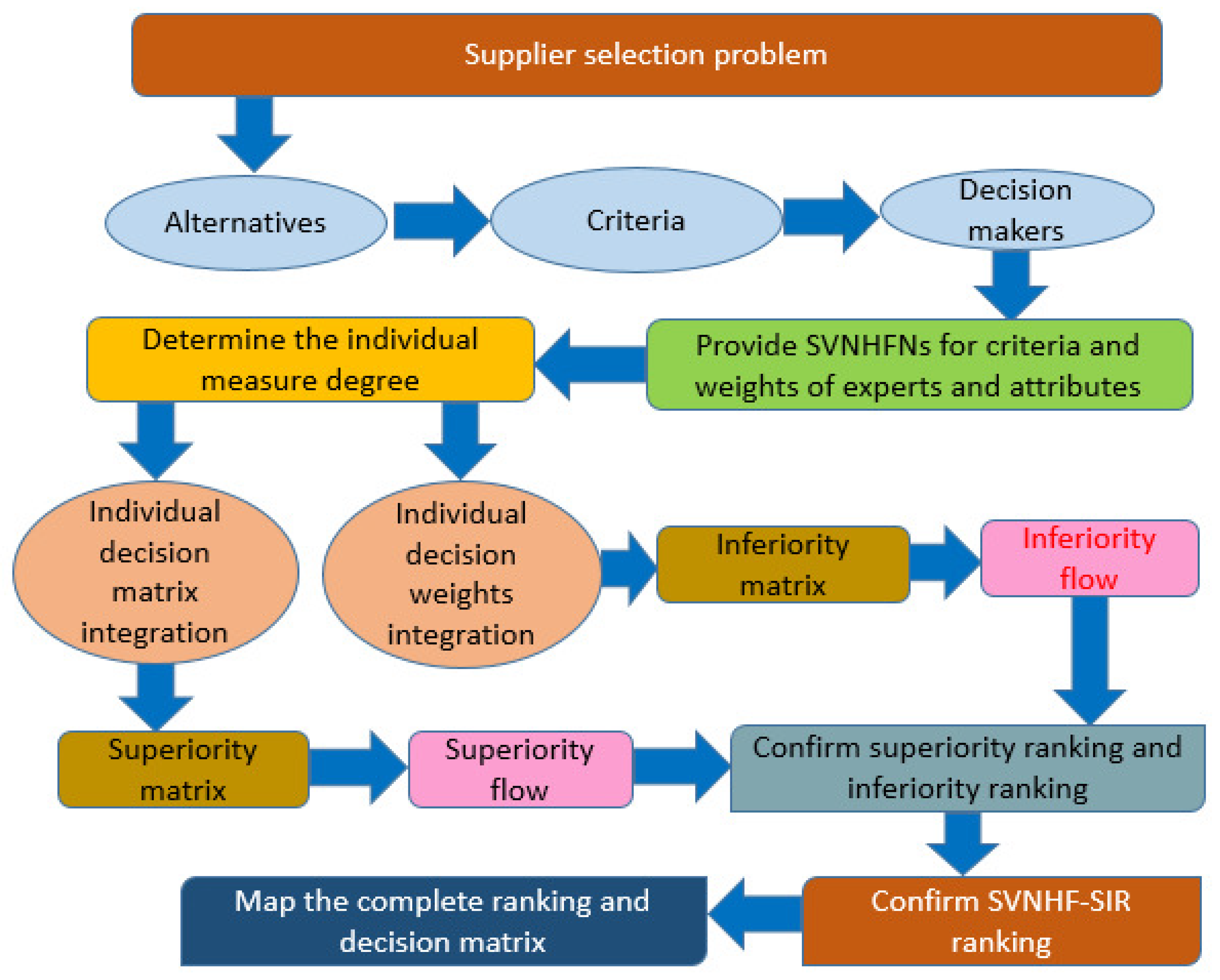
Inferiority ranking rule ($\mathcal{I}\mathcal{R}$-Rule): $\mathcal{I}\mathcal{R}-Rul{e}^1$. If ${\Psi }^{>}\left({\omega }_i^{\mathfrak{x}}\right)<{\Psi }^{>}\left({\omega }_{\mathfrak{t}}^{\mathfrak{x}}\right)$ and ${\Psi }^{<}\left({\omega }_i^{\mathfrak{x}}\right)>{\Psi }^{<}\left({\omega }_{\mathfrak{t}}^{\mathfrak{x}}\right)$, then ${\omega }_i^{\mathfrak{x}}\prec {\omega }_{\mathfrak{t}}^{\mathfrak{x}}$; $\mathcal{I}\mathcal{R}-Rul{e}^2$. If ${\Psi }^{>}\left({\omega }_i^{\mathfrak{x}}\right)<{\Psi }^{>}\left({\omega }_{\mathfrak{t}}^{\mathfrak{x}}\right)$ and ${\Psi }^{<}\left({\omega }_i^{\mathfrak{x}}\right)={\Psi }^{<}\left({\omega }_{\mathfrak{t}}^{\mathfrak{x}}\right)$, then ${\omega }_i^{\mathfrak{x}}\prec {\omega }_{\mathfrak{t}}^{\mathfrak{x}}$; $\mathcal{I}\mathcal{R}-Rul{e}^3$. If ${\Psi }^{>}\left({\omega }_i^{\mathfrak{x}}\right)={\Psi }^{>}\left({\omega }_{\mathfrak{t}}^{\mathfrak{x}}\right)$ and ${\Psi }^{<}\left({\omega }_i^{\mathfrak{x}}\right)>{\Psi }^{<}\left({\omega }_{\mathfrak{t}}^{\mathfrak{x}}\right)$, then ${\omega }_i^{\mathfrak{x}}\prec {\omega }_{\mathfrak{t}}^{\mathfrak{x}}$. Step 7: By incorporating the $\mathcal{S}\mathcal{R}$-Rule and the $\mathcal{I}\mathcal{R}$-Rule, we can achieve the best alternative ${\omega }_i^{\mathfrak{x}}(i=1,2,\cdots ,\mathfrak{l})$. A flow chart of the SIR method for supplier selection is shown in Figure 1.

Figure 1. Flow chart of SIR method for supplier selection.

Figure 1. Flow chart of SIR method for supplier selection.

5. Extension of CV Method for SVNHF Information

In this section, a new MCDM method is developed in Algorithm 2, which is extension of the CV method to SVNHFSs. Table 5 includes various types of cases where different systems were used to help with operations or decision-making in the food supply chain.

Algorithm 2: (CV method for SVNHFSs)

Step 1: Obtain the decision matrices from the decision makers, with alternative ${\omega }_j^{\mathfrak{x}}$ evaluated on the basis of criterion ${\omega }_i^{\mathbb{C}}$, given in Table 6. The aggregated decision matrix ${\overline{\mathfrak{p}}}_{ij}$ is obtained using step 1, step 2 and step $3\left(2\right)$. Step 2: Decision makers also give weight $\mathfrak{w}$ to the criteria with the condition that the sum of weights must be equal to 1. Then, the multiplication of decision matrix is computed with criteria weights, to obtain the matrix ${\overline{\mathfrak{q}}}_{ij}$. Step 3: Find the score function of each SVNHFN. Step 4: Compute the ranking of the alternatives according to their score function values.

Case Study

The food industry is critical for delivering the essentials for a variety of uses and tendencies [43]. Food must be stored, supplied, and marketed as soon as it is cultivated or produced so that it can reach the ultimate customers on time. Every year, worldwide food loss would supply more than enough to nourish the world’s nearly 1 billion starving people. In Pakistan, it is anticipated that $40\%$ of food is wasted. Food is produced in sufficient quantities to feed the overall population of Pakistan, but due to food waste, an expected 6 out of 10 inhabitants go to bed without dinner. Pakistan stands 107th out of 118 developing countries on the International Poverty Index. Approximately one-third of all produced food is destroyed or wasted each year (approximately $1.3$ billion tonnes) [44]. Two-thirds of all waste in food (roughly 1 billion tonnes) occurs at the supply chain stage, which encompasses cultivation, shipments, and storage [45].

The term FSCM has been utilized to depict the activities or procedures occurring during the yield, dispersion, and the use of various foods in order to preserve their quality and safety in effective and efficient ways [46,47]. The relevance of factors such as safety, food quality, and freshness within a specified time frame distinguishes FSCM from many other supply chains including furniture logistics and supply chain management, making the underpinning supply chain more convoluted and unmanageable [48]. As the challenges of global coordination have increased, the attention turned from a single echelon, such as food production, to the effectiveness and efficiency of the comprehensive supply chain. That is, the food supply chain resources such as vehicles, storage areas, transport services, and laborers will be used proficiently to ensure the quality and safety of food through effective efforts including optimization decisions [49]. The relevance of value chains in FSCM is that they benefit both consumers and producers. The traceability of food has become increasingly popular in recent decades, with a wide range of applications. Because of the emergence of food, FSCM is becoming more dynamic and complex in order to meet the diversifying and globalized industries.

FSCM IT Systems

There is no doubt that IT systems are crucial in FSCM because so much can go wrong, such as vehicles, food suppliers, data entry, and so on. The decision-making systems and traceability for FSCM are used as examples of current state-of-the-art situations that professionals can use when instituting IT-based solutions. A food’s traceability consists in a data trail that follows the physiological trail of the food through different phases [50]. Some systems track food all the way from the retailer to the farm, while others only examine key stages of the supply chain. Some traceability systems gather information only for tracking food products to the minute of manufacturing or logistics path, while others track only superficial data, such as in a vast geographical area [51]. Aside from FSCM’s traceability systems, other decision-making processes in the food industry include implementation, strategy, vehicle maintenance, and WMS.

The internationalization of food production, logistics, and utilization has resulted in an integrated world for FSCM, whose models are critical in ensuring consistently high standards and security in food products [52]. Quality of food, high delivery performance, and food security appear to be more important in these models. Multi-objective considerations are also common; for example, food quality assurance is incorporated into decision models. Recently, supply chain effectiveness and value chain evaluation have received special attention, since the international FSCM is becoming increasingly important.

Table 5. Cases involving IT systems in FSCM that have been reported.

Instance	Firm	Network	Enhancement
Aramyan et al. [53]	Tomato firm	Performance	Efficiency and flexibility
		measurement system	have both improved,
			food quality has improved,
			and there is a faster response time.
Bevilacqua et al. [54]	Tronto Valley	ARIS	Three types of costs
			are being reduced;
			improved traceability.
Pagell and Wu [55]	Pizza restaurants	TQM Lean/JIT	Enhanced information sharing,
			superior quality,
			enhanced logistical efficiency.
Tuncel and Alpan [56]	A medium size	Risk management	The percentage of orders completed
			on time has increased to $90.6\%$,
			with risk reduction rising by $9.9\%$.
Zhu et al. [57]	A food manufacturer	Customer cooperation	Customer cooperation has improved;
		system	internal environment management
			has been improved.
Jacxsens et al. [58]	A fresh producer	Food safety	Food of higher quality;
		management system	improved risk management ability.
Friel et al. [59]	Agri-food supply chain	H&S food	A more nutritious diet,
		decision-making	with improved environmental
		system	sustainability.
Savino et al. [60]	A chestnut	Value chain	Increased long-term viability,
	company	management	CO2 reduced emissions,
		system	enhanced value chain.
Banasik et al. [61]	A mushroom	Supply chain	Overall profitability increased by $11\%$,
	manufacturer	management	with improved environmental
		system	performance
Sgarbossa and Russo [62]	6 Firms	FSCM system	Conserving energy,
			costs of disposal avoided,
			enhanced productivity.

Table 5. Cases involving IT systems in FSCM that have been reported.

Instance	Firm	Network	Enhancement
Aramyan et al. [53]	Tomato firm	Performance	Efficiency and flexibility
		measurement system	have both improved,
			food quality has improved,
			and there is a faster response time.
Bevilacqua et al. [54]	Tronto Valley	ARIS	Three types of costs
			are being reduced;
			improved traceability.
Pagell and Wu [55]	Pizza restaurants	TQM Lean/JIT	Enhanced information sharing,
			superior quality,
			enhanced logistical efficiency.
Tuncel and Alpan [56]	A medium size	Risk management	The percentage of orders completed
			on time has increased to $90.6\%$,
			with risk reduction rising by $9.9\%$.
Zhu et al. [57]	A food manufacturer	Customer cooperation	Customer cooperation has improved;
		system	internal environment management
			has been improved.
Jacxsens et al. [58]	A fresh producer	Food safety	Food of higher quality;
		management system	improved risk management ability.
Friel et al. [59]	Agri-food supply chain	H&S food	A more nutritious diet,
		decision-making	with improved environmental
		system	sustainability.
Savino et al. [60]	A chestnut	Value chain	Increased long-term viability,
	company	management	CO2 reduced emissions,
		system	enhanced value chain.
Banasik et al. [61]	A mushroom	Supply chain	Overall profitability increased by $11\%$,
	manufacturer	management	with improved environmental
		system	performance
Sgarbossa and Russo [62]	6 Firms	FSCM system	Conserving energy,
			costs of disposal avoided,
			enhanced productivity.

Table 6. Single-valued neutrosophic hesitant fuzzy decision matrices.

${\omega }_1^{\mathfrak{e}}$	${\omega }_1^{\mathbb{C}}$	${\omega }_2^{\mathbb{C}}$	${\omega }_3^{\mathbb{C}}$
${\omega }_1^{\mathfrak{x}}$	$\{0.125,0.326\},\left\{0.444\right\},\left\{0.236\right\}$	$\left\{0.230\right\},\left\{0.200\right\},\left\{0.912\right\}$	$\left\{0.200\right\},\{0.111,0.253\},\left\{0.751\right\}$
${\omega }_2^{\mathfrak{x}}$	$\left\{0.111\right\},\{0.750,0.905\},\left\{0.216\right\}$	$\left\{0.250\right\},\left\{0.112\right\},\left\{0.445\right\}$	$\left\{0.523\right\},\left\{0.521\right\},\{0.423,0.624\}$
${\omega }_3^{\mathfrak{x}}$	$\left\{0.149\right\},\left\{0.242\right\},\left\{0.889\right\}$	$\{0.246,0.925\},\left\{0.851\right\},\left\{0.124\right\}$	$\{0.259,0.590\},\left\{0.125\right\},\left\{0.300\right\}$
${\omega }_4^{\mathfrak{x}}$	$\left\{0.195\right\},\left\{0.860\right\},\{0.120,0.120\}$	$\left\{0.315\right\},\left\{0.866\right\},\left\{0.606\right\}$	$\{0.400,0.580\},\left\{0.430\right\},\left\{0.118\right\}$
${\omega }_2^{\mathfrak{e}}$	${\omega }_1^{\mathbb{C}}$	${\omega }_2^{\mathbb{C}}$	${\omega }_3^{\mathbb{C}}$
${\omega }_1^{\mathfrak{x}}$	$\left\{0.326\right\},\left\{0.414\right\},\left\{0.216\right\}$	$\left\{0.655\right\},\left\{0.200\right\},\left\{0.219\right\}$	$\left\{0.800\right\},\left\{0.253\right\},\{0.715,0.870\}$
${\omega }_2^{\mathfrak{x}}$	$\left\{0.456\right\},\{0.570,0.800\},\left\{0.206\right\}$	$\left\{0.250\right\},\{0.102,0.436\},\left\{0.102\right\}$	$\left\{0.600\right\},\left\{0.500\right\},\left\{0.421\right\}$
${\omega }_3^{\mathfrak{x}}$	$\left\{0.419\right\},\left\{0.237\right\},\left\{0.900\right\}$	$\left\{0.380\right\},\left\{0.450\right\},\left\{0.120\right\}$	$\left\{0.529\right\},\left\{0.125\right\},\left\{0.210\right\}$
${\omega }_4^{\mathfrak{x}}$	$\left\{0.528\right\},\left\{0.111\right\},\{0.120,0.300\}$	$\left\{0.513\right\},\left\{0.750\right\},\left\{0.880\right\}$	$\left\{0.450\right\},\{0.400,0.500\},\left\{0.117\right\}$
${\omega }_3^{\mathfrak{e}}$	${\omega }_1^{\mathbb{C}}$	${\omega }_2^{\mathbb{C}}$	${\omega }_3^{\mathbb{C}}$
${\omega }_1^{\mathfrak{x}}$	$\{0.225,0.350\},\left\{0.420\right\},\left\{0.220\right\}$	$\left\{0.222\right\},\{0.150,0.215\},\left\{0.319\right\}$	$\left\{0.755\right\},\left\{0.253\right\},\left\{0.745\right\}$
${\omega }_2^{\mathfrak{x}}$	$\left\{0.330\right\},\left\{0.100\right\},\left\{0.498\right\}$	$\left\{0.546\right\},\left\{0.110\right\},\left\{0.623\right\}$	$\{0.550,0.600\},\left\{0.520\right\},\left\{0.324\right\}$
${\omega }_3^{\mathfrak{x}}$	$\left\{0.240\right\},\{0.230,0.300\},\left\{0.850\right\}$	$\left\{0.855\right\},\left\{0.114\right\},\left\{0.522\right\}$	$\left\{0.300\right\},\{0.100,0.550\},\left\{0.900\right\}$
${\omega }_4^{\mathfrak{x}}$	$\left\{0.800\right\},\left\{0.200\right\},\{0.120,0.300\}$	$\left\{0.356\right\},\left\{0.777\right\},\left\{0.415\right\}$	$\left\{0.444\right\},\left\{0.232\right\},\left\{0.718\right\}$

Table 6. Single-valued neutrosophic hesitant fuzzy decision matrices.

${\omega }_1^{\mathfrak{e}}$	${\omega }_1^{\mathbb{C}}$	${\omega }_2^{\mathbb{C}}$	${\omega }_3^{\mathbb{C}}$
${\omega }_1^{\mathfrak{x}}$	$\{0.125,0.326\},\left\{0.444\right\},\left\{0.236\right\}$	$\left\{0.230\right\},\left\{0.200\right\},\left\{0.912\right\}$	$\left\{0.200\right\},\{0.111,0.253\},\left\{0.751\right\}$
${\omega }_2^{\mathfrak{x}}$	$\left\{0.111\right\},\{0.750,0.905\},\left\{0.216\right\}$	$\left\{0.250\right\},\left\{0.112\right\},\left\{0.445\right\}$	$\left\{0.523\right\},\left\{0.521\right\},\{0.423,0.624\}$
${\omega }_3^{\mathfrak{x}}$	$\left\{0.149\right\},\left\{0.242\right\},\left\{0.889\right\}$	$\{0.246,0.925\},\left\{0.851\right\},\left\{0.124\right\}$	$\{0.259,0.590\},\left\{0.125\right\},\left\{0.300\right\}$
${\omega }_4^{\mathfrak{x}}$	$\left\{0.195\right\},\left\{0.860\right\},\{0.120,0.120\}$	$\left\{0.315\right\},\left\{0.866\right\},\left\{0.606\right\}$	$\{0.400,0.580\},\left\{0.430\right\},\left\{0.118\right\}$
${\omega }_2^{\mathfrak{e}}$	${\omega }_1^{\mathbb{C}}$	${\omega }_2^{\mathbb{C}}$	${\omega }_3^{\mathbb{C}}$
${\omega }_1^{\mathfrak{x}}$	$\left\{0.326\right\},\left\{0.414\right\},\left\{0.216\right\}$	$\left\{0.655\right\},\left\{0.200\right\},\left\{0.219\right\}$	$\left\{0.800\right\},\left\{0.253\right\},\{0.715,0.870\}$
${\omega }_2^{\mathfrak{x}}$	$\left\{0.456\right\},\{0.570,0.800\},\left\{0.206\right\}$	$\left\{0.250\right\},\{0.102,0.436\},\left\{0.102\right\}$	$\left\{0.600\right\},\left\{0.500\right\},\left\{0.421\right\}$
${\omega }_3^{\mathfrak{x}}$	$\left\{0.419\right\},\left\{0.237\right\},\left\{0.900\right\}$	$\left\{0.380\right\},\left\{0.450\right\},\left\{0.120\right\}$	$\left\{0.529\right\},\left\{0.125\right\},\left\{0.210\right\}$
${\omega }_4^{\mathfrak{x}}$	$\left\{0.528\right\},\left\{0.111\right\},\{0.120,0.300\}$	$\left\{0.513\right\},\left\{0.750\right\},\left\{0.880\right\}$	$\left\{0.450\right\},\{0.400,0.500\},\left\{0.117\right\}$
${\omega }_3^{\mathfrak{e}}$	${\omega }_1^{\mathbb{C}}$	${\omega }_2^{\mathbb{C}}$	${\omega }_3^{\mathbb{C}}$
${\omega }_1^{\mathfrak{x}}$	$\{0.225,0.350\},\left\{0.420\right\},\left\{0.220\right\}$	$\left\{0.222\right\},\{0.150,0.215\},\left\{0.319\right\}$	$\left\{0.755\right\},\left\{0.253\right\},\left\{0.745\right\}$
${\omega }_2^{\mathfrak{x}}$	$\left\{0.330\right\},\left\{0.100\right\},\left\{0.498\right\}$	$\left\{0.546\right\},\left\{0.110\right\},\left\{0.623\right\}$	$\{0.550,0.600\},\left\{0.520\right\},\left\{0.324\right\}$
${\omega }_3^{\mathfrak{x}}$	$\left\{0.240\right\},\{0.230,0.300\},\left\{0.850\right\}$	$\left\{0.855\right\},\left\{0.114\right\},\left\{0.522\right\}$	$\left\{0.300\right\},\{0.100,0.550\},\left\{0.900\right\}$
${\omega }_4^{\mathfrak{x}}$	$\left\{0.800\right\},\left\{0.200\right\},\{0.120,0.300\}$	$\left\{0.356\right\},\left\{0.777\right\},\left\{0.415\right\}$	$\left\{0.444\right\},\left\{0.232\right\},\left\{0.718\right\}$

Choosing a supplier is a critical element of any business’s operations. Reputation, reliability, service, cost, and value for money are all important considerations. The aim of supplier selection is to identify the best supplier who delivers the best value for money in terms of product or service. Suitable supplier selection yields good profit and quality in the end. The supplier is treated as an integral part of the organization in this strategic alliance. All purchasers must choose a supplier, and it is a critical step in the acquisition process. Purchasers should go through several stages of decision making and develop their own selection criteria for selecting appropriate suppliers.

Some interesting studies for supply chain can be seen in [63,64,65].

6. MCDM Process

The RH Flour Mills in Lahore wants to find the best supplier for one of its key components in the manufacturing process. Four suppliers were left as alternatives. The four criteria considered were: quality and safety, delivery, social responsibility, and service. The suppliers are evaluated using the recommended methodology by a group of decision makers. In multi-criteria decision making with a fuzzy environment, four decision makers were chosen, consisting of supplier experts and expert academics. The steps in the procedure for selecting the best green supplier are as follows.

The decision-making process using Algorithm 1 is illustrated as follows:

Let $\mathcal{K}=\{{\omega }_1^{\mathfrak{x}},{\omega }_2^{\mathfrak{x}},{\omega }_3^{\mathfrak{x}},{\omega }_{\mathfrak{4}}^{\mathfrak{x}}\}$ is the set of alternatives and $\mathbb{C}=\{{\omega }_1^{\mathbb{C}},{\omega }_2^{\mathbb{C}},{\omega }_{\mathfrak{3}}^{\mathbb{C}}\}$ is the set of attributes. Assume that $\mathfrak{E}=\{{\omega }_1^{\mathfrak{e}},{\omega }_2^{\mathfrak{e}},{\omega }_{\mathfrak{3}}^{\mathfrak{e}}\}$ is the set of experts. Then, the single-valued neutrosophic hesitant fuzzy decision matrices are expressed in Table 6, the weights of the experts are given in

Table 7. The weights of the experts.

Experts	SVNHFEs
${\omega }_1^{\mathfrak{e}}$	$\{0.831,0.120\},\left\{0.310\right\},\{0.456,0.511\}$
${\omega }_2^{\mathfrak{e}}$	$\left\{0.802\right\},\{0.408,0.300\},\left\{0.472\right\}$
${\omega }_3^{\mathfrak{e}}$	$\{0.711,0.177\},\{0.234,0.500\},\{0.500,0.250\}$

, and the weights of the attributes are shown in

Table 8. The weights of the attributes.

	${\mathit{\omega }}_1^{\mathbb{C}}$	${\mathit{\omega }}_2^{\mathbb{C}}$	${\mathit{\omega }}_3^{\mathbb{C}}$
${\omega }_1^{\mathfrak{e}}$	$\left\{0.311\right\},\left\{0.200\right\},\left\{0.500\right\}$	$\{0.111,0.210\},\left\{0.100\right\},\left\{0.805\right\}$	$\{0.200,0.666\},\left\{0.555\right\},\left\{0.213\right\}$
${\omega }_2^{\mathfrak{e}}$	$\left\{0.207\right\},\{0.300,0.804\},\left\{0.274\right\}$	$\left\{0.750\right\},\left\{0.455\right\},\left\{0.123\right\}$	$\left\{0.100\right\},\left\{0.578\right\},\left\{0.920\right\}$
${\omega }_3^{\mathfrak{e}}$	$\{0.170,0.701\},\left\{0.230\right\},\left\{0.240\right\}$	$\left\{0.380\right\},\{0.335,0.510\},\left\{0.200\right\}$	$\left\{0.310\right\},\{0.456,0.687\},\left\{0.836\right\}$

.

Step 1: Compute the individual measure degree ${\rho }_k(k=1,2,3)$ using Equation (6), given by

$$\rho ={(0.432,0.466,0.573)}^{\mu }$$

Step 2: Acquire the normalized vector using Equation (7), given as

$$\varpi ={(0.294,0.317,0.390)}^{\mu }$$

Step 3: The attribute weights can be obtained using Equation (8), which are expressed as follows:

$$\begin{array}{c}\hfill {\dot{\mathfrak{w}}}_1=\left(\{0.226,0.480\},\{0.240,0.328\},\left\{0.310\right\}\right)\\ \hfill {\dot{\mathfrak{w}}}_2=\left(\{0.483,0.501\},\{0.258,0.304\},\left\{0.258\right\}\right)\\ \hfill {\dot{\mathfrak{w}}}_3=\left(\{0.216,0.394\},\{0.520,0.611\},\left\{0.576\right\}\right)\end{array}$$

The aggregated decision matrices can be obtained using Equation (9), and can be written as follows:

$${\left({\mathfrak{p}}_{ij}\right)}_{4\times 3}=\left(\begin{array}{ccc}\{0.232,0.283,0.289,0.336\},\left\{0.425\right\},\left\{0.223\right\}& \left\{0.401\right\},\{0.178,0.205\},\left\{0.385\right\}& \left\{0.675\right\},\{0.198,0.253\},\{0.737,0.784\}\\ \left\{0.319\right\},\{0.313,0.349,0.331,0.369\},\left\{0.294\right\}& \left\{0.384\right\},\{0.108,0.171\},\left\{0.318\right\}& \{0.559,0.579\},\left\{0.514\right\},\{0.380,0.426\}\\ \left\{0.279\right\},\{0.253,0.261\},\left\{0.877\right\}& \{0.628,0.811\},\left\{0.317\right\},\left\{0.215\right\}& \{0.372,0.473\},\{0.114,0.222\},\left\{0.411\right\}\\ \left\{0.605\right\},\left\{0.254\right\},\{0.120,0.171,0.359,0.215\}& \left\{0.400\right\},\left\{0.793\right\},\left\{0.588\right\}& \{0.434,0.490\},\{0.330,0.354\},\left\{0.237\right\}\end{array}\right)$$

Step 4: Acquire the performance function ${\mathfrak{f}}_{ij}$ using Equation (10):

$${\left({\mathfrak{f}}_{ij}\right)}_{4\times 3}=\left(\begin{array}{ccc}0.586& 0.540& 0.464\\ 0.625& 0.644& 0.599\\ 0.179& 0.767& 0.688\\ 1& 0.198& 0.601\end{array}\right)$$

The threshold attribute function was set to

$${\varphi }_k\left(d\right)=\left\{\begin{array}{cc}0.01\hfill & ifd>0\hfill \\ 0.00\hfill & ifd\le 0\hfill \end{array}\right.$$

Acquire the superiority matrix ($\mathcal{S}$-matrix) using Equation (12):

$$\mathcal{S}=\left(\begin{array}{ccc}0.01& 0.01& 0\\ 0.02& 0.02& 0.01\\ 0& 0.03& 0.03\\ 0.03& 0& 0.02\end{array}\right)$$

Acquire the inferiority matrix ($\mathcal{I}$-matrix) using Equation (13):

$$\mathcal{I}=\left(\begin{array}{ccc}0.02& 0.02& 0.03\\ 0.01& 0.01& 0.02\\ 0.03& 0& 0\\ 0& 0.03& 0.01\end{array}\right)$$

Step 5: Measure the flow of superiority and inferiority using Equations (14) and (15), which are exhibited in

Table 9. SVNHF superiority flow.

	${\mathbf{\Psi }}^{>}\left({\mathit{\omega }}_{\mathit{i}}^{\mathfrak{x}}\right)$	$\mathbb{S}\left({\mathbf{\Psi }}^{>}\left({\mathit{\omega }}_{\mathit{i}}^{\mathfrak{x}}\right)\right)$
${\omega }_1^{\mathfrak{x}}$	$\{0.00709,0.00981\},\{0.00498,0.00632\},\left\{0.00568\right\}$	$0.6657$
${\omega }_2^{\mathfrak{x}}$	$\{0.01634,0.02356\},\{0.01516,0.01875\},\left\{0.01712\right\}$	$0.6619$
${\omega }_3^{\mathfrak{x}}$	$\{0.02097,0.02685\},\{0.02334,0.02745\},\left\{0.02502\right\}$	$0.6597$
${\omega }_4^{\mathfrak{x}}$	$\{0.0111,0.02228\},\{0.0176,0.02206\},\left\{0.02082\right\}$	$0.6587$

and

Table 10. SVNHF inferiority flow.

	${\mathbf{\Psi }}^{<}\left({\mathit{\omega }}_{\mathit{i}}^{\mathfrak{x}}\right)$	$\mathbb{S}\left({\mathbf{\Psi }}^{<}\left({\mathit{\omega }}_{\mathit{i}}^{\mathfrak{x}}\right)\right)$
${\omega }_1^{\mathfrak{x}}$	$\{0.02066,0.03144\},\{0.02556,0.03097\},\left\{0.02864\right\}$	$0.6564$
${\omega }_2^{\mathfrak{x}}$	$\{0.01175,0.01769\},\{0.01538,0.01854\},\left\{0.0172\right\}$	$0.6602$
${\omega }_3^{\mathfrak{x}}$	$\{0.00678,0.0144\},\{0.0072,0.00984\},\left\{0.0093\right\}$	$0.6643$
${\omega }_4^{\mathfrak{x}}$	$\{0.01665,0.01897\},\{0.01294,0.01523\},\left\{0.0135\right\}$	$0.6634$

.

Step 6: Integrate Table 9 with the $\mathcal{S}\mathcal{R}$-Rule, and the following seems to be accessible:

$${\omega }_1^{\mathfrak{x}}\succ {\omega }_2^{\mathfrak{x}}\succ {\omega }_3^{\mathfrak{x}}\succ {\omega }_4^{\mathfrak{x}}$$

Combine Table 10 with the $\mathcal{I}\mathcal{R}$-Rule, and the following seems to be accessible:

$${\omega }_1^{\mathfrak{x}}\succ {\omega }_2^{\mathfrak{x}}\succ {\omega }_4^{\mathfrak{x}}\succ {\omega }_3^{\mathfrak{x}}$$

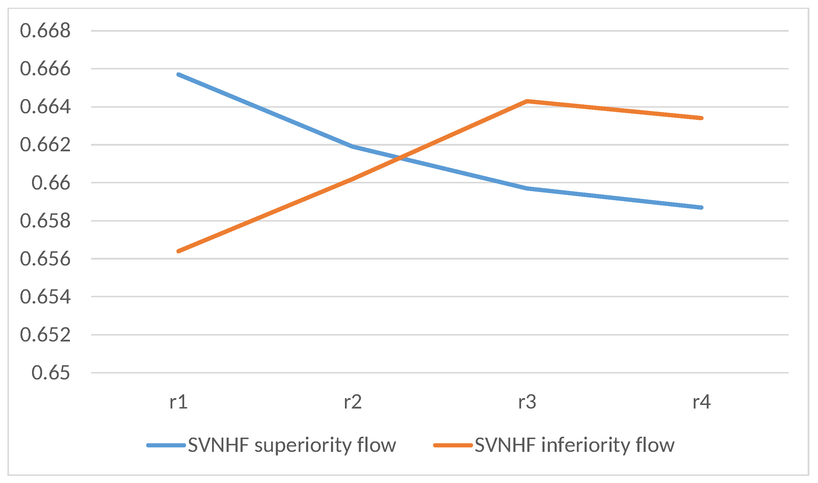
Step 7: The most desirable alternative, according to the results of the $\mathcal{S}\mathcal{R}$-Rule and the $\mathcal{I}\mathcal{R}$-Rule, is ${\omega }_1^{\mathfrak{x}}$. A representation of SVNHF superiority and inferiority flow is shown in Figure 2.

The decision-making process using Algorithm 2 is illustrated as follows: Step 1: Consider SVNHF decision matrices given in Table 6. Obtain aggregated decision matrix ${\left({\overline{\mathfrak{p}}}_{ij}\right)}_{4\times 3}$ using Step 1, Step 2, and Step 3. Step 2: The decision makers provide weights to three criteria as ${\mathfrak{w}}_1=0.235$, ${\mathfrak{w}}_2=0.312$, and ${\mathfrak{w}}_3=0.453$, with $\sum {\mathfrak{w}}_i=1$

$${\left({\overline{\mathfrak{q}}}_{ij}\right)}_{4\times 3}=\left(\begin{array}{ccc}\{0.232,0.283,0.289,0.336\},\left\{0.425\right\},\left\{0.223\right\}& \left\{0.401\right\},\{0.0.178,0.205\},\left\{0.385\right\}& \left\{0.675\right\},\{0.0.198,0.253\},\{0.737,0.784\}\\ \left\{0.319\right\},\{0.313,0.349,0.331,0.369\},\left\{0.294\right\}& \left\{0.384\right\},\{0.108,0.171\},\left\{0.318\right\}& \{0.559,0.579\},\left\{0.514\right\},\{0.380,0.426\}\\ \left\{0.279\right\},\{0.253,0.261\},\left\{0.877\right\}& \{0.628,0.811\},\left\{0.317\right\},\left\{0.215\right\}& \{0.372,0.473\},\{0.114,0.222\},\left\{0.411\right\}\\ \left\{0.605\right\},\left\{0.254\right\},\{0.120,0.171,0.359,0.215\}& \left\{0.400\right\},\left\{0.793\right\},\left\{0.588\right\}& \{0.434,0.490\},\{0.330,0.354\},\left\{0.237\right\}\end{array}\right)\left(\begin{array}{c}0.235\\ 0.312\\ 0.453\end{array}\right)$$

$${\left({\overline{\mathfrak{q}}}_{ij}\right)}_{4\times 1}=\left(\begin{array}{c}\{0.484,0.495,0.496,0.507\},\{0.0005,0.0007\},\{0.0021,0.0022\}\\ \{0.446,0.455\},\{0.0006,0.0006,0.0006,0.0011\},\{0.0017,0.0013\}\\ \{0.429,0.529\},\{0.0003,0.0006\},\left\{0.0026\right\}\\ \{0.461,0.485\},\{0.0022,0.0024\},\{0.0005,0.0008,0.0016,0.0010\}\end{array}\right)$$

Step 3: Compute the score values of each alternative. The score values of the alternatives are given in

Table 11. Score values.

Alternatives	Score Values
${\omega }_1^{\mathfrak{x}}$	0.8309
${\omega }_2^{\mathfrak{x}}$	0.8158
${\omega }_3^{\mathfrak{x}}$	0.8253
${\omega }_4^{\mathfrak{x}}$	0.8233

.

Step 4: Rank the alternatives according to their score values.

$$\begin{array}{c}\hfill {\omega }_1^{\mathfrak{x}}\succ {\omega }_3^{\mathfrak{x}}\succ {\omega }_4^{\mathfrak{x}}\succ {\omega }_2^{\mathfrak{x}}\end{array}$$

As a result, ${\omega }_1^{\mathfrak{x}}$ is the best supplier among the four alternatives according to the qualities of all criteria.

Comparative Analysis

This paper develops new techniques for modeling uncertainties using SVNHF information. We compare the ranking of alternatives using proposed SIR method and the CV method for SVNHFSs. If we use the SVNHF SIR approach to assemble the alternatives, they are ranked for superiority flow as

$${\omega }_1^{\mathfrak{x}}\succ {\omega }_2^{\mathfrak{x}}\succ {\omega }_3^{\mathfrak{x}}\succ {\omega }_4^{\mathfrak{x}}$$

and for inferiority flow as

$${\omega }_1^{\mathfrak{x}}\succ {\omega }_2^{\mathfrak{x}}\succ {\omega }_4^{\mathfrak{x}}\succ {\omega }_3^{\mathfrak{x}}$$

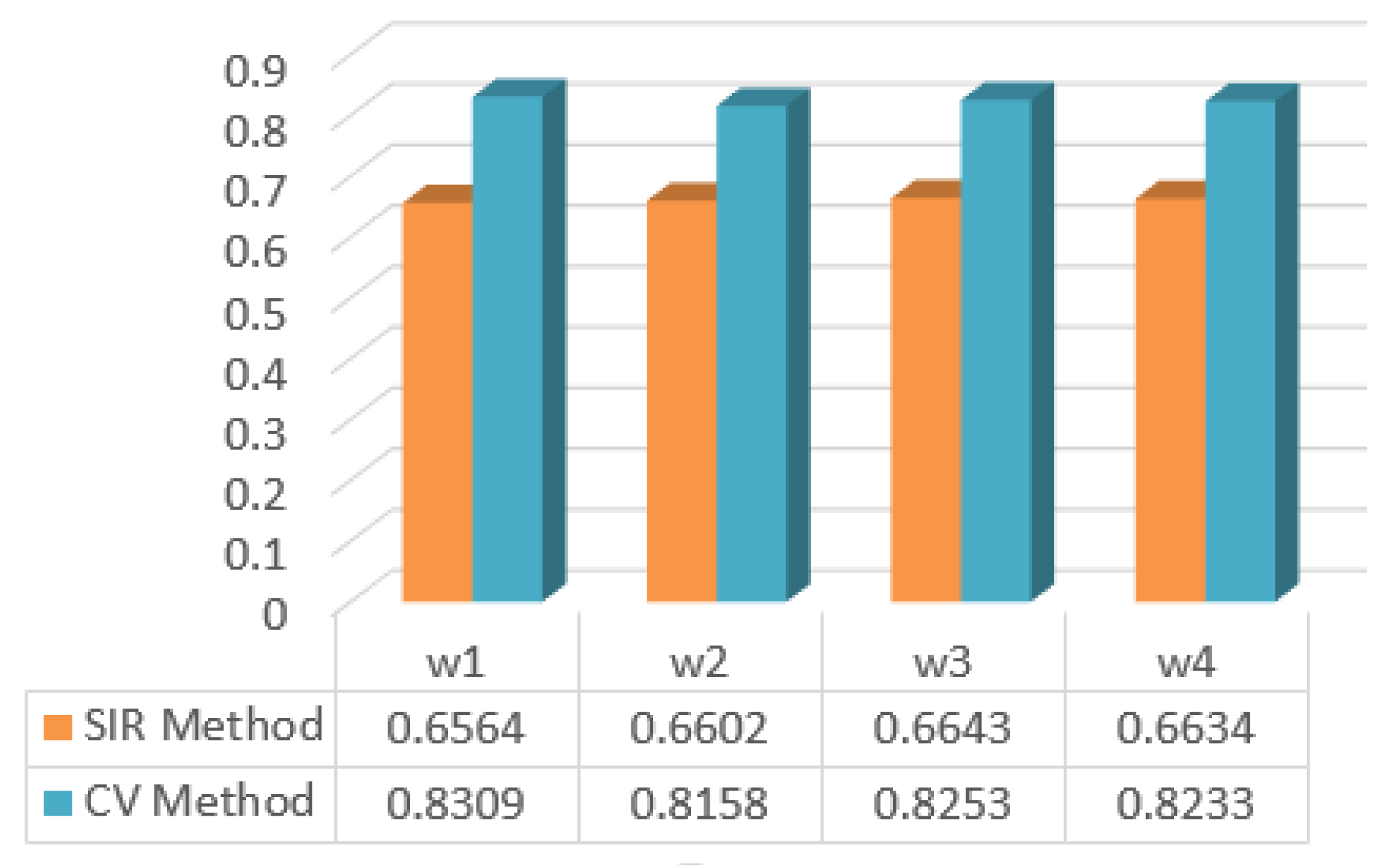
On the other hand, when we use the technique of the CV method, the ranking of the alternatives becomes

$${\omega }_1^{\mathfrak{x}}\succ {\omega }_3^{\mathfrak{x}}\succ {\omega }_4^{\mathfrak{x}}\succ {\omega }_2^{\mathfrak{x}}$$

Based on these findings, it is clear that the ranking of the alternatives is not same. However, the optimal alternative ${\omega }_1^{\mathfrak{x}}$ remains identical in both MCDM methods.

The ranking of alternatives using the SIR method and the CV method is also shown in Figure 3.

7. Conclusions

This paper was designed to introduce the concept of single-valued neutrosophic hesitant fuzzy (SVNHF) topology and its applications in data analysis for uncertain supply chains. An SVNHFS is a hybrid structure of a hesitant fuzzy set (HFS) and a single-valued neutrosophic set (SVNS), which is a novel concept for modeling uncertainties in real-life circumstances with key features of three membership functions: truth-hesitancy membership function, indeterminacy-hesitancy membership function and falsity-hesitancy membership function. Using the characteristics of SVNHFSs, we defined the notion of SVNHF topology. We investigated the fundamental properties of SVNHF topology, such as the SVNHF closure, the SVNHF interior, the SVNHF exterior, and the SVNHF frontier, as well as the SVNHF dense set and the SVNHF base, with the help illustrative examples. Eventually, to demonstrate and validate the SIR method and the CV method in terms of rationality and scientific basis, a real-life example of supplier selection in a food supply chain was provided. A comparative analysis was also given to discuss the validity and advantage of proposed techniques. The proposed methods can be further extended to investigate the dynamics of human decision analysis, humanized computing, data analysis, computational intelligence, and healthcare.

References

- Zadeh, L.A. Fuzzy sets. Inf. Control. 1965, 8, 338–353. [Google Scholar] [CrossRef] [Green Version]
- Atanassov, T.K. Intuitionistic fuzzy sets. Fuzzy Sets Syst. 1986, 20, 87–96. [Google Scholar] [CrossRef]
- Yager, R.R. Pythagorean fuzzy subsets. In Proceedings of the Joint IFSA World Congress and NAFIPS Annual Meeting, Edmonton, AB, Canada, 24–28 June 2013; pp. 57–61. [Google Scholar]
- Yager, R.R. Generalized orthopair fuzzy sets. IEEE Trans. Fuzzy Syst. 2017, 25, 1222–1230. [Google Scholar] [CrossRef]
- Cuong, B.C. Picture fuzzy sets. J. Comput. Sci. Cybern. 2014, 30, 409–420. [Google Scholar]
- Mahmood, T.; Ullah, K.; Khan, Q.; Jan, N. An approach toward decision-making and medical diagnosis problems using the concept of spherical fuzzy sets. Neural Comput. Appl. 2019, 31, 7041–7053. [Google Scholar] [CrossRef]
- Ashraf, S.; Abdullah, S.; Mahmood, T.; Ghani, F.; Mahmood, T. Spherical fuzzy sets and their applications in multi-attribute decision making problems. J. Intell. Fuzzy Syst. 2019, 36, 2829–2844. [Google Scholar] [CrossRef]
- Gündogdu, F.K.; Kahraman, C. Spherical fuzzy sets and spherical fuzzy TOPSIS method. J. Intell. Fuzzy Syst. 2018, 36, 337–352. [Google Scholar] [CrossRef]
- Smarandache, F. A Unifying Field in Logics: Neutrosophy: Neutrosophic Probability, Set and Logic; American Research Press: Rehoboth, DE, USA, 1999; pp. 1–141. [Google Scholar]
- Wang, H.; Smarandache, F.; Zhang, Y.; Sunderraman, R. Single-Valued Neutrosophic Sets; Infinite Study: Coimbatore, India, 2010; pp. 1–4. [Google Scholar]
- Molodtsov, D. Soft set theory-first results. Comput. Math. Appl. 1999, 37, 19–31. [Google Scholar] [CrossRef] [Green Version]
- Hashmi, M.R.; Riaz, M.; Smarandache, F. m-polar Neutrosophic Topology with Applications to Multi-Criteria Decision-Making in Medical Diagnosis and Clustering Analysis. Int. J. Fuzzy Syst. 2020, 22, 273–292. [Google Scholar] [CrossRef]
- Torra, V. Hesitant fuzzy sets. Int. J. Intell. Syst. 2010, 25, 529–539. [Google Scholar] [CrossRef]
- Ye, J. Multiple-attribute Decision-Making Method under a Single-Valued Neutrosophic Hesitant Fuzzy Environment. J. Intell. Syst. 2015, 24, 23–36. [Google Scholar] [CrossRef]
- Tanuwijaya, B.; Selvachandran, G.; Son, L.H.; Basset, M.A.; Huynh, H.X.; Pham, V.H.; Ismail, M. A Novel Single Valued Neutrosophic Hesitant Fuzzy Time Series Model: Applications in Indonesian and Argentinian Stock Index Forecasting. IEEE Access 2020, 8, 60126–60141. [Google Scholar] [CrossRef]
- Liu, C.F.; Luo, Y.S. New aggregation operators of single-valued neutrosophic hesitant fuzzy set and their application in multi-attribute decision making. Pattern Anal. Appl. 2019, 22, 417–427. [Google Scholar] [CrossRef]
- Wang, R.; Li, Y. Generalized Single-Valued Neutrosophic Hesitant Fuzzy Prioritized Aggregation Operators and Their Applications to Multiple Criteria Decision-Making. Information 2018, 9, 10. [Google Scholar] [CrossRef] [Green Version]
- Giri, B.C.; Molla, M.U.; Biswas, P. TOPSIS Method for Neutrosophic Hesitant Fuzzy Multi-Attribute Decision Making. Informatica 2020, 31, 35–63. [Google Scholar] [CrossRef]
- Xu, X. The SIR method: A superiority and inferiority ranking method for multiple criteria decision making. Eur. J. Oper. Res. 2001, 131, 587–602. [Google Scholar] [CrossRef]
- Tam, C.M.; Tong, T.K.L.; Wong, Y.W. Selection of concrete pump using the superiority and inferiority ranking method. J. Constr. Eng. Manag. 2004, 130, 827–834. [Google Scholar] [CrossRef]
- Tam, C.M.; Tong, T.K. Locating large-scale harbourfront project developments using SIR method with grey aggregation approach. Constr. Innov. 2008, 8, 120–136. [Google Scholar] [CrossRef]
- Chai, J.; Liu, J.N.K. A Novel Multicriteria Group Decision Making Approach with Intuitionistic Fuzzy SIR Method. In Proceedings of the World Automation Congress, Kobe, Japan, 19–23 September 2010. [Google Scholar]
- Ma, Z.J.; Zhang, N.; Dai, Y. A novel SIR method for multiple attributes group decision making problem under hesitant fuzzy environment. J. Intell. Fuzzy Syst. 2014, 26, 2119–2130. [Google Scholar] [CrossRef]
- Peng, X.; Yang, Y. Some results for Pythagorean fuzzy sets. Int. J. Intell. Syst. 2015, 30, 1133–1160. [Google Scholar] [CrossRef]
- Rouhani, S. A fuzzy superiority and inferiority ranking based approach for IT service management software selection. Kybernetes 2017, 46, 728–746. [Google Scholar] [CrossRef]
- Chen, T. A novel PROMETHEE-based outranking approach for multiple criteria decision analysis with Pythagorean fuzzy information. IEEE Access 2018, 6, 54495–54506. [Google Scholar] [CrossRef]
- Tavana, M.; Zareinejad, M.; Arteaga, F.J.S. An intuitionistic fuzzy-grey superiority and inferiority ranking method for third-party reverse logistics provider selection. Int. J. Syst. Sci. Oper. Logist. 2018, 5, 175–194. [Google Scholar] [CrossRef]
- Zhao, N.; Xu, Z.; Ren, Z. Hesitant fuzzy linguistic prioritized superiority and inferiority ranking method and its application in sustainable energy technology evaluation. Inf. Sci. 2019, 478, 239–257. [Google Scholar] [CrossRef]
- Geetha, S.; Narayanamoorthy, S. Superiority and inferiority ranking method with hesitant Pythagorean fuzzy set for solving MCDM problems. Malaya J. Mat. 2020, 1, 11–15. [Google Scholar]
- Jian, J.; Zhan, N.; Su, J. A novel superiority and inferiority ranking method for engineering investment selection under interval-valued intuitionistic fuzzy environment. J. Intell. Fuzzy Syst. 2019, 37, 6645–6653. [Google Scholar] [CrossRef]
- Smarandache, F. New types of Neutrosophic Set/Logic/Probability, Neutrosophic Over-/Under-/Off-Set, Neutrosophic Refined Set, and their Extension to Plithogenic Set/Logic/Probability, with Applications; MDPI: Basel, Switzerland, 2019. [Google Scholar]
- Seikh, M.R.; Dutta, S. A Nonlinear Programming Model to Solve Matrix Games with Pay-offs of Single-valued Neutrosophic Numbers. Neutrosophic Sets Syst. 2021, 47, 366–383. [Google Scholar]
- Saha, A.; Paul, A. Generalized Weighted Exponential Similarity Measures of Single Valued Neutrosophic Sets. Int. J. Neutrosophic Sci. 2019, 0, 57–66. [Google Scholar]
- Alcantud, J.C.R.; Garcia, G.S.; Akram, M. OWA aggregation operators and multi-agent decisions with N-soft sets. Expert Syst. Appl. 2022, 203, 1–17. [Google Scholar]
- Sitara, M.; Akram, M.; Riaz, M. Decision-making analysis based on q-rung picture fuzzy graph structures. J. Appl. Math. Comput. 2021, 67, 541–577. [Google Scholar] [CrossRef]
- Riaz, M.; Riaz, M.; Jamil, N.; Zararsiz, Z. Distance and similarity measures for bipolar fuzzy soft sets with application to pharmaceutical logistics and supply chain management. J. Intell. Fuzzy Syst. 2022, 42, 3169–3188. [Google Scholar] [CrossRef]
- Farid, H.M.A.; Riaz, M. Some generalized q-rung orthopair fuzzy Einstein interactive geometric aggregation operators with improved operational laws. Int. J. Intell. Syst. 2021, 36, 7239–7273. [Google Scholar] [CrossRef]
- Zararsiz, Z.; Riaz, M. Bipolar fuzzy metric spaces with application. Comput. Appl. Math. 2022, 41, 41–49. [Google Scholar] [CrossRef]
- Riaz, M.; Tanveer, S.; Pamucar, D.; Qin, D.S. Topological data analysis with spherical fuzzy soft AHP-TOPSIS for environmental mitigation system. Mathematics 2022, 10, 1826. [Google Scholar] [CrossRef]
- Riaz, M.; Farid, H.M.A.; Wang, W.; Pamucar, D. Interval-valued linear Diophantine fuzzy Frank aggregation operators with multi-criteria decision-making. Mathematics 2022, 10, 1811. [Google Scholar] [CrossRef]
- Biswas, P.; Pramanik, S.; Giri, B.C. GRA Method of Multiple Attribute Decision Making with Single Valued Neutrosophic Hesitant Fuzzy Set Information. In New Trends in Neutrosophic Theory and Applications; Pons Editions: Brussels, Belgium, 2016. [Google Scholar]
- Brans, J.P.; Vincke, P.; Mareschal, B. How to select and how to rank projects: The PROMETHEE method. Eur. J. Oper. Res. 1986, 24, 228–238. [Google Scholar] [CrossRef]
- Cooper, M.C.; Ellram, L.M. Characteristics of supply chain management and the implications for purchasing and logistics strategy. Int. J. Logist. Manag. 1993, 4, 13–24. [Google Scholar] [CrossRef]
- Manning, L.; Baines, R.; Chadd, S. Quality assurance models in the food supply chain. Br. Food J. 2006, 108, 91–104. [Google Scholar] [CrossRef]
- Fritz, M.; Schiefer, G. Food chain management for sustainable food system development: A European research agenda. Agribusiness 2008, 24, 440–452. [Google Scholar] [CrossRef]
- Blandon, J.; Henson, S.; Cranfield, J. Small-scale farmer participation in new agri-food supply chains: Case of the supermarket supply chain for fruit and vegetables in Honduras. J. Int. Dev. 2009, 21, 971–984. [Google Scholar] [CrossRef]
- Marsden, T.; Banks, J.; Bristow, G. Food supply chain approaches: Exploring their role in rural development. Sociol. Rural. 2000, 40, 424–438. [Google Scholar] [CrossRef]
- Scalia, G.L.; Settanni, L.; Micale, R.; Enea, M. Predictive shelf life model based on RF technology for improving the management of food supply chain: A case study. Int. J. Technol. 2016, 7, 31–42. [Google Scholar] [CrossRef]
- Wu, K.J.; Liao, C.J.; Tseng, M.; Chiu, K.K.S. Multi-attribute approach to sustainable supply chain management under uncertainty. Ind. Manag. Data Syst. 2016, 116, 777–800. [Google Scholar] [CrossRef]
- Smith, G.; Tatum, J.; Belk, K.; Scanga, J.; Grandin, T.; Sofos, J. Traceability from a US perspective. Meat Sci. 2005, 71, 174–193. [Google Scholar] [CrossRef]
- Dickinson, D.L.; Bailey, D. Meat traceability: Are US consumers willing to pay for it? J. Agric. Resour. Econ. 2002, 27, 348–364. [Google Scholar]
- Choi, T.M.; Chiu, C.H.; Chan, H.K. Risk management of logistics systems. Transp. Res. Logist. Transp. Rev. 2016, 90, 1–6. [Google Scholar] [CrossRef]
- Aramyan, L.H.; Lansink, A.G.O.; Vorst, J.G.V.D.; Van Kooten, O. Performance measurement in agri-food supply chains: A case study. Supply Chain. Manag. Int. J. 2007, 12, 304–315. [Google Scholar] [CrossRef]
- Bevilacqua, M.; Ciarapica, F.; Giacchetta, G. Business process reengineering of a supply chain and a traceability system: A case study. J. Food Eng. 2009, 93, 13–22. [Google Scholar] [CrossRef]
- Pagell, M.; Wu, Z. Building a more complete theory of sustainable supply chain management using case studies of 10 exemplars. J. Supply Chain. Manag. 2009, 45, 37–56. [Google Scholar] [CrossRef]
- Tuncel, G.; Alpan, G. Risk assessment and management for supply chain networks: A case study. Comput. Ind. 2010, 61, 250–259. [Google Scholar] [CrossRef]
- Zhu, Q.H.; Geng, Y.; Fujita, T.; Hashimoto, S. Green supply chain management in leading manufacturers: Case studies in Japanese large companies. Manag. Res. Rev. 2010, 33, 380–392. [Google Scholar] [CrossRef]
- Jacxsens, L.; Luning, P.; Vorst, J.V.D.; Devlieghere, F.; Leemans, R.; Uyttendaele, M. Simulation modelling and risk assessment as tools to identify the impact of climate change on microbiological food safety—The case study of fresh produce supply chain. Food Res. Int. 2010, 43, 1925–1935. [Google Scholar] [CrossRef]
- Friel, S.; Barosh, L.J.; Lawrence, M. Towards healthy and sustainable food consumption: An Australian case study. Public Health Nutr. 2014, 17, 1156–1166. [Google Scholar] [CrossRef] [Green Version]
- Savino, M.M.; Manzini, R.; Mazza, A. Environmental and economic assessment of fresh fruit supply chain through value chain analysis: A case study in chestnuts industry. Prod. Plan. Control. 2015, 26, 1–18. [Google Scholar] [CrossRef]
- Banasik, A.; Kanellopoulos, A.; Claassen, G.; Bloemhof-Ruwaard, J.M.; Vorst, J.G.V.D. Closing loops in agricultural supply chains using multi-objective optimization: A case study of an industrial mushroom supply chain. Int. J. Prod. Econ. 2017, 183, 409–420. [Google Scholar] [CrossRef]
- Sgarbossa, F.; Russo, I. A proactive model in sustainable food supply chain: Insight from a case study. Int. J. Prod. Econ. 2017, 183, 596–606. [Google Scholar] [CrossRef]
- Tzounis, A.; Katsoulas, N.; Bartzanas, T.; Kittas, C. Internet of Things in agriculture, recent advances and future challenges. Biosyst. Eng. 2017, 164, 31–48. [Google Scholar] [CrossRef]
- Feng, F.; Jun, Y.B.; Liu, X.; Li, L. An adjustable approach to fuzzy soft set based decision making. J. Comput. Appl. Math. 2010, 234, 10–20. [Google Scholar]
- Zhong, R.; Xu, X.; Wang, L. Food supply chain management: Systems, implementations, and future research. Ind. Manag. Data Syst. 2017, 117, 2085–2114. [Google Scholar] [CrossRef]
Figure 2.
Representation of SVNHF superiority and inferiority flow.
Figure 3.
Ranking of alternatives using the SIR method and the CV method.