
Runtime Software Architecture-Based Reliability Prediction for Self-Adaptive Systems


1
School of Reliability and Systems Engineering, Beihang University, Beijing 100191, China
2
National Key Laboratory of Science and Technology on Reliability and Environmental Engineering, Beijing 100191, China
*
Authors to whom correspondence should be addressed.
Symmetry 2022, 14(3), 589; https://doi.org/10.3390/sym14030589
Submission received: 1 March 2022
/
Revised: 11 March 2022
/
Accepted: 14 March 2022
/
Published: 16 March 2022
(This article belongs to the Topic Dynamical Systems: Theory and Applications)
Abstract
:Modern software systems need to autonomously adapt their behavior at runtime in order to maintain their utility in response to continuous environmental changes. Most studies on models at runtime focus on providing suitable techniques to manage the complexity of software at runtime but neglect reliability caused by adaptation activities. Therefore, adaptive behaviors may lead to a decrease in reliability, which may result in severe financial loss or life damage. Runtime software architecture (RSA) is an abstract of a running system, which describes the elements of the current system, the states of these elements and the relation between the elements and their states at runtime. The main difference between RSA and software architecture at design time (DSA) is that RSA has a causal connection with the running system, whereas DSA does not. However, RSA and DSA have both symmetry and asymmetry in software architecture. To ensure that architecture-centric software can provide reliable services after adaptation adjustment, a method is proposed to analyze the impact of changes caused by adaptation strategy on the overall software reliability, which will be predicted at the runtime architecture model layer. Based on a Java platform, through non-intrusive monitoring, an RSA behavioral model is obtained followed by runtime reliability analysis model. Following this, reliability prediction results are obtained through a discrete-time Markov chain (DTMC). Finally, an experiment is conducted to verify the feasibility of the proposed method.
1. Introduction
With the prevalence of network and computing technology, today’s world features a growing number of new software applications such as ultra-large-scale (ULS) systems, ubiquitous computing, cyber-physical systems (CPS) and distributed systems [1,2], which greatly increase the dependence on software. Meanwhile, the software runtime environment has changed from closed, static and controllable to open, dynamic and uncertain, which makes software often face external and self-inflicted variation during runtime. For example, cloud-based applications need to modify their behavior during operation in response to increasing events, such as resource interruption, peak load, infrastructure changes or third-party services [3]. Subsequently, self-adaptation has become an inevitable demand for modern software systems to continually provide services and achieve necessary dynamicity [4,5].
A self-adaptive software system responds to runtime changes by establishing an adaptive strategy, which refers to a planning method used to manipulate the system’s state, structure and behavior changes [6]. However, most existing self-adaptive software offer passive or static adaptation, which the software designers predefine at the design stage and do as much as possible to deal with those changes before the system is implemented. This kind of adaptation, therefore, may become dated during runtime due to the uncertainty of environment conditions, especially for sustainable software applications in big data, cloud computing and mobile internet environments. Moreover, most existing strategies attach importance to examining the logical correctness of adaptation, ignoring its impact on the reliability of the target system. Therefore, strategies may lead to a degradation or destroying of the reliability of the target system. Therefore, how to automatically predict the runtime reliability of the target system for each adaptation strategy is a challenging and difficult problem.
The software architecture model has a profound effect on the software life-span and has become one of the most common means of handling the complexity of self-adaptive systems from a high-level review of the systems [7]. Architectural adaptations can be structural, behavioral or both. Structural adaptations refer to the changes of system architectural topology and its constituent elements (e.g., adding or deleting components or connectors). Two alternative services with the same interface but different reliability are provided, so structural adaptation can give varied reliability to the target system. Behavioral adaptations aim at the changes of behavior of each architectural element and the interaction between architectural elements. For instance, by changing the interaction protocol between two services from synchronous to asynchronous mode, behavioral adaptation may change the reliability of the resulting system [8].
An RSA model can, therefore, be divided into an RSA structural model and an RSA behavioral model. Of these, the RSA structural model focuses on describing the composition and configuration of the underlying system, i.e., emphasizing how the software is built. For example, in terms of an object-oriented technique, the RSA structural model describes the inheritance relationship and calling path, components and their connections. The RSA behavioral model, by contrast, focuses on describing the dynamic interaction between components, emphasizing system execution based on events or tracking processes, or the occurrence and execution of events, i.e., the behavioral model describes event arrival, queuing, selection and schedule etc.
Moreover, many reliability predictions based on DSA were provided by existing studies. RSA and DSA have both symmetry and asymmetry. Both are description forms of architecture, with the same constituent elements and forms, but DSA embodies a static architecture, which cannot be changed at runtime, and lacks a mechanism for expressing dynamic updates. RSA is a dynamic architecture with dynamic features such as constructability and adaptability. Therefore, existing reliability prediction methods based on DSA cannot solve the problem of reliability prediction at runtime, because there is a great difference between the actual RSA and DSA; moreover, with the operation of the software, the changes of the surrounding environments and the driving of different adaptive strategies, there are more and more deviations between RSA and DSA. Judging the possible impact of each strategy on reliability needs to be carried out for each specific strategy. As a result, the existing reliability prediction methods based on DSA cannot meet the demand.
To address the above-mentioned challenges, in this paper, we propose a runtime reliability prediction method, that is, how to obtain the runtime architecture model, which includes the structural model and the behavioral model, and how to collect the data related to the reliability at runtime, so as to realize the transformation from the runtime architecture model to the reliability analysis model. Based on the reliability analysis model, the quantitative reliability prediction results driven by the adaptation strategy are obtained to evaluate the impact of the adaptive strategies on the reliability of the target system during operation and effectively avoid the unacceptable results with the execution of those strategies on target system reliability, which provides a basis or reference for active adaptive strategy selection from the perspective of reliability.
The proposed approach can be used in the field of infrastructures supporting the realization of self-adaptive systems. The existing infrastructures are designed to ensure the adaptive behavior of the runtime system driven by the adaptive strategies, emphasizing the logical consistency between the runtime model and the runtime system with its environment, but ignoring the reliability of the target system that the adaptive implementation may result in reducing. Therefore, the proposed method provides a complementary mechanism to compensate for the above shortcomings, which ensures that the adaption action does not affect the reliability of target system. Generally speaking, the reliability measure used in this method can be regarded as “Reliability”, which is the probability that the software/component will work without failure for a specified period of time, e.g., the reliability of a component can be defined as the maximum rate of requests it may reliably serve, and adaptation actions can be adding, deleting and replacing components or connectors and so on.
The main contributions of our work are listed as follows.
- We propose a method for constructing the software runtime architecture model, which includes a runtime architecture structural model and a behavioral model. The architecture structural model contains data about the topology of the system, and the behavioral model can be obtained by monitoring the target system to get the observations for updating the behavioral model at runtime according to the adaptation strategy.
- We present a technique to construct a reliability prediction-oriented analysis model. The reliability of components and the transition probability between components are added to obtain the prediction-oriented runtime reliability expansion model, then through model conversion, the prediction-oriented runtime reliability expansion model is converted into a Markov analysis model.
- We provide a method to obtain the reliability prediction result at runtime through the Markov analysis model.
- We conduct an experimental study based on rainbow-znn software to show the effectiveness of the proposed approach.
2. Related Work
The aim of our work is to develop an RSA-based reliability prediction method that takes into consideration the impact on reliability of the system after the implementation of the adaptive strategy, and effectively avoids the execution of decisions that may adversely affect the reliability of the system. Therefore, hereafter, we review works appearing in the literature dealing with (i) software reliability prediction based on DSA, (ii) the conception of RSA, (iii) infrastructure for RSA construction, (iv) adaptive strategy and its verification method, and (v) methods to guarantee the properties of self-adaptive system.
Software reliability prediction based on DSA. Architecture-based approaches for software reliability prediction have been proposed over the last three decades [9]. during this time, software architecture refers to DSA, which consists of a set of components, connectors and configurations, and describes the structures of software at an abstract level [10]. It includes many styles such as batch-sequential style, parallel/pipe-filter style, fault tolerance and call-and-return style, along with new styles constantly emerging, whose frameworks are to characterize the configurations of components and connectors [11]. All DSA can be identified according to the design specification of a system and the main task related to DSA is to select the suitable styles to model and predict software reliability to ensure design quality at the early design stage of the software development life cycle.
Conception of RSA. The concept of an RSA was first proposed by Oreizy [12], who described the evolution of the system during operation based on the C2 architectural style. Software runtime model is the representation of the underlying system that are both self-representation and causally connected. It emphasizes the structure, behavior or goal of the target system from the perspective of problem space and connects an architectural model to a running system. Such a connection is the key to M@RT-based systems (M@RT is short for model at runtime), since it allows one to maintain a runtime model for a running system. The software runtime model provides an abstraction of the running system, which can be used to fix design errors or fold new design decisions into the system. Strategies are mapped into the running system to support controlled ongoing design [13]. At the same time, the runtime model, as the foundation of software evolution and adaptive behavior [14], is also the key to solve the problem of runtime management for complex systems [15]. Gordon [13] and Bencomo [16] proposed that the runtime model is a self-representation that has a causal connection with the target system. The so-called causal connection between the runtime model and the target system means that when the target system changes, the runtime model should also change, and vice versa. It can, thus, be seen that the biggest difference between RSA model and DSA model is that there is a causal connection between RSA and the runtime system, while DSA does not have this attribute.
Infrastructure for the construction of RSA. An RSA model focuses on how to describe the current structure and configuration of the running system [17,18,19]. Thus, the development of appropriate infrastructure is considered to be very important to maintain the causal relationship between the target system and its RSA [20]. Representative works include the Rainbow framework provided by Carnegie Mellon University [21], MADAM for mobile applications designed by Floch [22], and PKUAS [23] and SM@RT [20] proposed by Peking University for runtime architecture construction infrastructure. The Rainbow framework automatically generates the runtime architecture model of the controlled object in the form of snapshots, describing the system composition of the controlled object at the current moment when the snapshot is generated and the cross-linking relationship between the constituent elements, but only emphasizes the current runtime system’s structure and configuration. SM@RT is a runtime architecture generation framework based on general architecture and system synchronization technology. The runtime architecture model can be used to predict and analyze the quality attributes at the model level, but currently there are only studies related to performance prediction, such as response time without reliability prediction [17]. In addition, Morin et al. [24] applied model-level aspect to encapsulate and manage the variants. Elkhodary et al. [25] provided a feature-oriented adaptive framework FUSION, which can learn the influence of the adaptive decision on system objectives. D’Ippolito et al. [26] presented a multi-layer control framework for adaptive system, which can adapt to the function of a system by degradation or enhancement. Chen et al. [27] put forward combining requirement and architectural adaptation through model transformation at runtime.
Although the above infrastructures provide fundamental mechanisms for the realization of adaptable systems, it is still too difficult to adapt the runtime system for changes within an acceptable reliability level, because the infrastructures only solve the problem of “how to do”, but cannot answer “why, when and what to do” during the adaptation, because they do not know what information should be collected for any given quality attributes [28].
Adaptive strategy and its verification method. Adaptive strategy is an abstraction of the behavior that the software system should adopt under specific conditions. When the adaptive strategy acts on the target system, the resulting execution result directly affects the running system. How to verify the adaptive strategy to ensure the reliability of the target system is one of the key challenges in the domain of self-adaptive software [29]. Currently, most existing verifications of adaptive strategies focus on validation of the logical consistency, that is, consistency among multiple runtime models and fidelity of runtime models with respect to the running system and its environment. For example, [30] uses model checking, such as time automata, and checking tools to analyze whether the controller has deadlock and connectivity to the control process. The reconfiguration impact of adaptive software is evaluated based on the idea of combination testing [31]. A reconfiguration sequence that does not meet the constraint conditions will be removed by the generation of a combination of variable points, and the obtained reconfiguration sequence set will be used as the decision-making module. The set of alternatives reduce the probability of unreliable strategies in the decision-making process. The reconfiguration strategy is executed on a copy of the architecture model, and the feasibility of the strategy execution on the target system is ensured by judging whether the model copy meets the constraints [32]. By importing specific scenarios, expected goals and the sequence of strategies to be tested into the simulation platform, the execution effects of the strategies are monitored to determine whether the strategies can guarantee the realization of the system goals in different scenarios [33]. However, most of the methods for model verification focus on verifying security, fairness and consistency of the software architecture, while other quality attributes such as availability and reliability are not involved. It is not conducive to analyse the system, nor can the quality of the software system be guaranteed.
Method to guarantee the properties of self-adaptive system. In order to guarantee the properties of the self-adaptive systems, mathematical models and formal methods have attracted more and more attention, such as Petri Nets [34], layered queuing networks [35], Markov chains [36] and timed automata [37], together with formal verification (e.g., PRISM [38] and UPPAAL [39]). Filieri et al. [40] provided KAMI to afford continuous assurance of performance requirements based on Markov models. Alternative implementations are modeled as different transitions that exit a given state with different probabilities in discrete-time Markov chains [41]. Chen et al. updated probability and quality values in the behavioral specification and performed behavioral adaptations with automatically generated alternatives, which support relaxed functional constraints from the perspective of business value [8]. Calinecu et al. utilized Markov chains to model system behaviors and adjust behavior parameters by exhaustive and quantitative verification to maximize a multi-objective utility strategy [42]. They also put forward QoSMOS to optimize service-oriented systems [43]. Ghezzi et al. provided a framework, ADAM, to manage nonfunctional uncertainty, which uses a Markov decision process to model adaptive systems with optional functions and functionality implementations [44]. Moreno et al. developed an active delay-sensitive adaptation method that considers the random behavior of the environment, which uses a Markov decision process to specify adaptive decisions and probabilistic model checking to solve the runtime decisions [45].
Summarizing, this paper proposes, with respect to existing work, the following:
- A reliability prediction method based on RSA instead of DSA.
- An approach that leverages the Rainbow framework for the construction of an RSA structural model, then the construction of the RSA behavioral model.
- A way to analyze the impact of changes caused by adaptive strategies on the overall software reliability.
3. Method Development
3.1. The Principle of the Method
3.1.1. Time
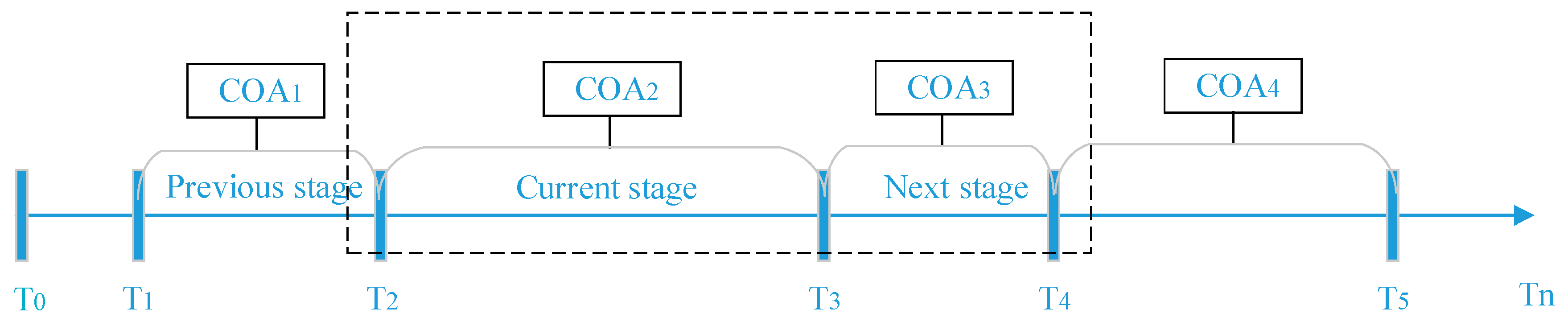
Figure 1 provides an overview of our method’s application time. The horizontal axis represents the running time of the entire execution process, including the start time T0, the adaptation trigger times T1, T2, T3 and so on, representing the trigger time of the first cycle of adaptation (COA1), the second cycle of adaptation (COA2), the third cycle of adaptation (COA3), respectively. Tn represents the end time of the execution. The entire adaptation process is then divided into several cycles of adaptation, e.g., COA1 to COA4.
Suppose COA2 is the current adaptation stage and COA3 is the next adaptation stage, the aim of our method is to provide the reliability prediction for the next adaptation stage COA3, but in the current adaptation stage COA2. That is, the time to carry out the reliability prediction is not when COA3 is really coming, but in COA2 and the runtime model for COA3 is obtained by inference and the overall reliability of the target software in COA3 is predicted according to the runtime model for COA3.
3.1.2. Mechanism
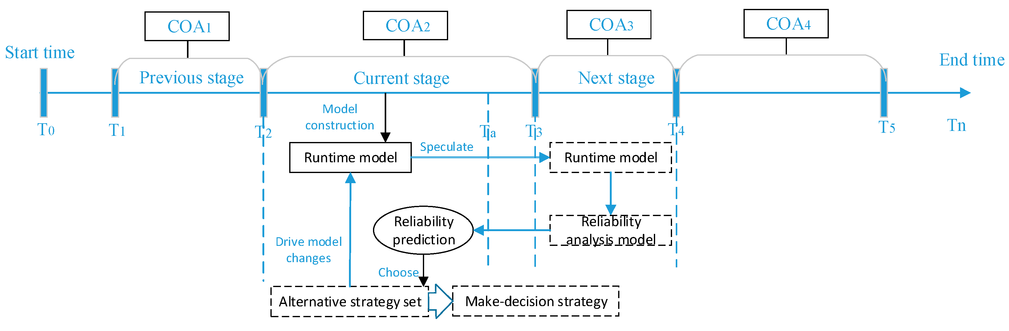
Figure 2 gives an overview of our method’s mechanism. When the system enters the current adaptation stage COA2 and before time Ta, the runtime model in COA2 is obtained by the method of model construction. At the same time, following the possible adaptation strategy alternative, the runtime model of COA2 is driven to change in order to obtain the runtime model of COA3. It should be noted that the runtime model of COA3 is represented in the dotted rectangles shown in Figure 2, which means that the runtime model of COA3 is obtained by inference based on the runtime model of COA2. After that, the reliability of the components in the model and the relationship between components can be used to predict the overall reliability of the software in the stage of COA3. Since there are multiple strategy alternatives at the moment when this adaptation strategy is triggered, after all reliability prediction results are calculated, one strategy needs to be selected according to the final prediction results, i.e., the strategy with the highest reliability is selected to drive the software to self-adapt. It should be noted that the entire method is carried out only after time T2 and before time Ta.
Here the reliability of the system is denoted as R, namely the probability that the system can carry out tasks successfully without failures, which is selected as the parameter of runtime reliability prediction result.
3.1.3. Process
The entire adaptation process can be described as follows.
Firstly, construct the runtime structural model according to steady state during the current stage.
Secondly, construct the runtime behavioral model.
Thirdly, according to the adaptation strategy and the changes of the software running environments, the runtime model (structural model and behavior model combined) is driven to change, and the runtime model for reliability prediction is inferred.
Next, add the information of components’ reliability and the transition probability between components to obtain the expansion model for reliability prediction.
After model conversion, the expansion model is converted into a Markov analysis model, which is used to obtain the reliability prediction results.
Finally, according to the reliability prediction results, one strategy is determined and recommended.
Obviously, there are five models involved in the whole procedure, which are RSA structural model (RSASM), RSA behavioral model (RSABM), the runtime model for reliability prediction (RMRP), the runtime model with reliability extensions (PRMRE) and Markov analysis model.
3.2. Key Steps
3.2.1. Step 1: Construct RSA Structural Model (RSASM)
RSASM contains data about the topology of the system, which describe the system composition and configuration at the current moment. According to the infrastructure supported by reflective middleware, we can directly obtain the model. The description of the structural model is also an essential requirement for the functional requirement, and many existing studies on infrastructure have undertaken much work and achieved very good results.
In our method, we, therefore, illustrate and validate our proposal with the aid of Rainbow, which is a platform for architecture-based self-adaptation [46]. We utilize Rainbow’s snapshot mechanism to obtain the RSASM. For example, Figure 3 provides a snapshot for rainbow-znn software, which gives the topology of the system.
It should be noted that here the construction of the RSASM is based on the Java reflection mechanism, so the applicable object of this method is limited to the software developed on Java. In addition, because this method is proposed in the context of software architecture, we use the Rainbow runtime model snapshot mechanism to obtain the monitored objects, which are the EJB components corresponding to the components in the runtime model generated by the Rainbow framework.
3.2.2. Step 2: Construct RSA Behavioral Model (RSABM)
This includes the following steps.
- According to the RSASM, determine the objects to be monitored.
- Declare the proxy bean while monitoring; this corresponds to the application bean and has the same remote interface as the application bean.
- Declare the monitor bean, which completes the extraction of dynamic component call information, which, in turn, includes the call relationship, the number of calls between components and the call timing.
- Declare the interface between the proxy bean and the monitor bean which have been established in 2 and 3.
- Construct the RSABM basing it on the model construction algorithm, which is shown in Algorithm 1.
| Algorithm 1 Pseudo-code for the RSA behavioral model construction algorithm. |
| Input: The invocation sequence of components, list. The format of each line is: Caller:Callee The original invocation timestamp list, timeList. The format of each line is: ComponentName:IN/OUT: TimeStamp Output: The adjacent matrix of component invocation, invMat 1 Initiate empty stack stackInv and stackTmp; 2 preComp←column 1 of the first element in list; 3 for each line in list do 4 compName←column 1 of line; 5 notation←colunm 2 of line; 6 if notation = ’IN’ then 7 Push compName in stackInv; 8 if Rows of invMat contains compName then 9 Increase the value at row preComp, column compName by 1; 10 end 11 else 12 Add a row and a column in invMat with compName as the name; 13 Set the value at row preComp, column compName as 0; 14 end 15 preComp←compName; 16 end 17 if notation = ’OUT’ then 18 topElement←Pop out the element on top of stackInv; 19 if topElement = compName then 20 Pop out each element in stackTmp and push it into stackInv; 21 end 22 else 23 Set the value at row preComp, column compName as negative; 24 Set the value at row preComp, column topElement as negative; 25 Push topElement in stackTmp; 26 Return to 18 27 end 28 preComp←the element left on top of stackInv 29 end 30 end |
Thus, from the above two steps, we can obtain the runtime model for the RSA.
3.2.3. Step 3: Construct a Reliability Prediction-Oriented Runtime Model (RMRP)
After building the RSABM, the set of adaptive strategies can be applied to drive it to change, after which models with reliability extension are inferred. Specifically, the construction process of the RMRP will be given, along with its formal description. During the entire prediction process, the RMRP must provide the necessary information for the subsequent Markov analysis model. This information includes the following.
- Structure information, i.e., what components are composed of the software.
- Relationship of caller and callee between components.
- The number of calls and transition modes between components. The determination of the transition probability between components is affected by the number of calls and the transfer mode between components, therefore, the number of calls and the transfer mode should also be given in RMRP.
Moreover, an RMRP also needs to describe the structural relationship between components. The transition mode is defined as the structural relationship when multiple components are called in the actual execution process. Here the component transfer modes include three styles: sequential mode, conditional mode and concurrent mode. As shown in Table 1, the transition modes are graphically represented based on the description of the branch nodes in the UML activity diagram.
The sequential transition can be regarded as when the components are executed in a sequential manner. For the branch structure, the possible component transition modes include concurrent mode and conditional mode. Take components A, B and C, for instance, to illustrate the difference between these two different transfer modes. The concurrent transfer mode can be taken as when Component A calls C, while calling B simultaneously. The conditional transfer mode can be regarded as when A first calls B, then transits the control authority to A after the execution of B is completed, or A calls C first, then returns the control authority to A after C’s execution ends. The loop structure can be described as a special judgment action; therefore, the transfer mode under the loop structure is also a conditional transfer mode.
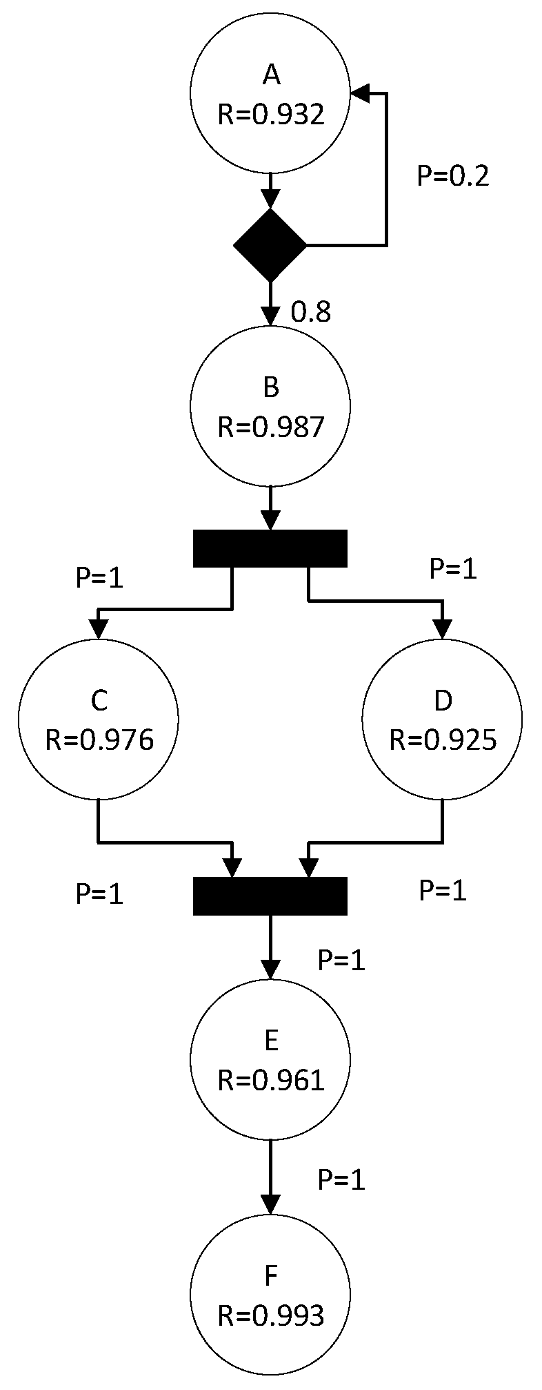
Based on the above transfer modes, a schematic diagram of the RMRP is given in Figure 4.
The construction process of the RMRP includes the following three steps.
- Construct the RSABM running in the current adaptation phase
Firstly, obtain the RSASM of the current phase through the Rainbow framework, which focuses on describing the system composition and configuration at the current moment. Next, through real-time monitoring of the controlled objects provided by the monitor, collect all kinds of information related to the monitored objects, complete the extraction of component dynamic call information, and realize the construction of RSABM.
- 2.
- Determine the adaptive strategies
Because reliability prediction is driven by different adaptive strategies to predict the overall reliability after adaptation, the adaptive strategies are selected from the set of alternative strategies which will be stated when the environmental conditions actually change.
- 3.
- Acquire the RMRP on the basis of the RSABM and adaptive strategies
The adaptive strategies are applied to the RSABM to drive the system to change, following which, the RMRP model is inferred. Thus, the changes of the RSABM include the following three aspects. The first is the change in the structure and behavior, such as adding and deleting components, or the calling relationship between components changing from synchronous calling to asynchronous calling, etc. The second is the change of component transfer mode, such as changing from the sequential transfer mode to the concurrent one. The third is the change in the number of component calls.
For modeling changes in the structure and behavior of runtime model, the extended UML multi-view method can be used. For the change of component transfer mode, it is usually determined and realized by the adaptation strategy.
A series of rules for the component transfer mode change are given below, where a formal description is given to improve the accuracy of the modeling process. Specifically, when a certain operation of the adaptation strategy is performed, the transfer mode between components changes from the source mode to the target mode. This rule is called action–transition mode change rule (ATMC).
The operations include adding, deleting, replacing components and changing the way the message is called. The source mode represents the transfer mode between the architectural components before the rule is applied, and the target mode represents the transfer mode after the rule is applied.
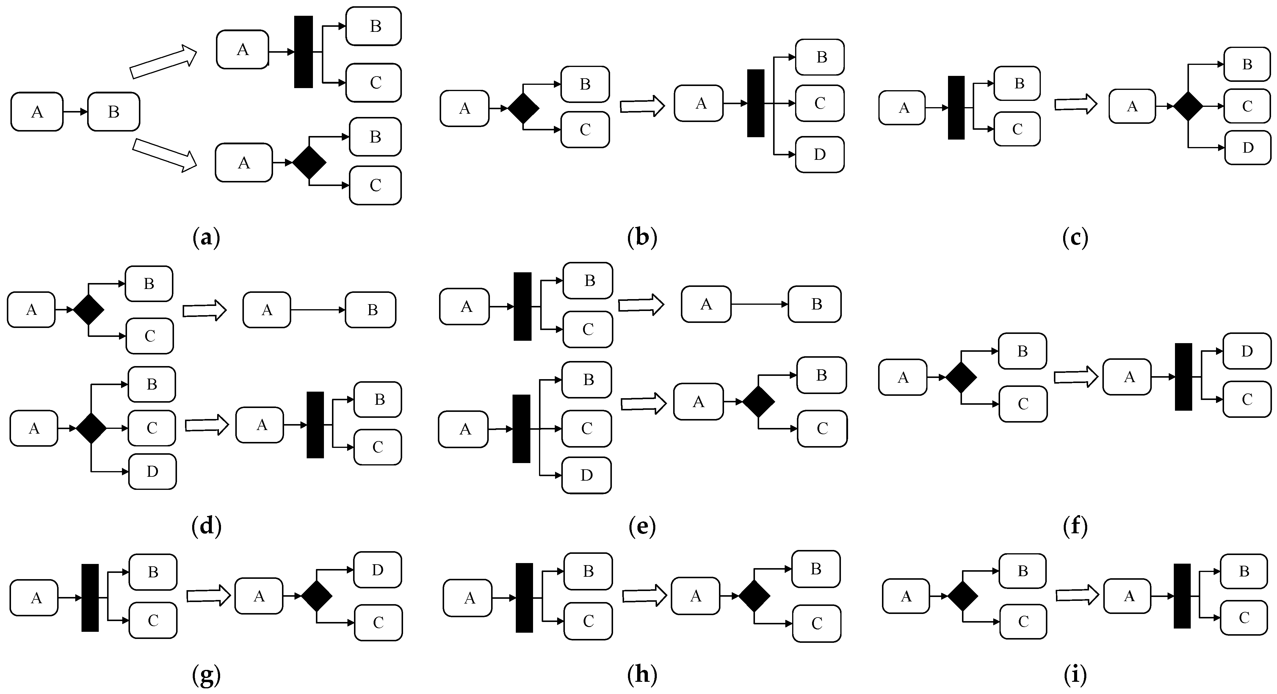
Figure 5a–c illustrates the change of the sequential transfer mode, the conditional transition mode and the concurrent transfer mode under the operation of adding a component. For example, in Figure 5a, adding a component may change the sequential transfer mode to the concurrent transfer mode or the conditional transfer mode.
Similarly, Figure 5d,e illustrates the change of the conditional transfer mode and the concurrent transfer mode under the operation of deleting a component.
Likewise, Figure 5f,g illustrates the change of the conditional and concurrent transfer modes under the operation of replacing a component.
The connector parameter refers to the parameter related to the message calling mode and its corresponding operation that changes the message calling mode, which can change the transfer mode between the components without changing the composition and structure of the architecture. Figure 5h,i shows the change of the concurrent and conditional transfer mode under the operation of changing the message call mode.
Thus, the transfer mode between nodes in RSABM can be marked according to the above nine rules and the RMRP can be built accordingly.
Among the three component transfer modes of RMRP, only the component transfer probability in the conditional transfer mode is related to the number of calls between components and the transfer mode. The transfer probability needs to be calculated by the number of calls between the components, while for the sequential and concurrent transfer mode, it is considered that it has nothing to do with the number of calls between components.
Through modeling the adaptive changes, the RSABM components after the implementation of the adaptation strategy are divided into two categories. The first category is the reserved components retained by RSABM, and the second category is newly added components after the implementation of the adaptation strategy.
In addition, two concepts need to be introduced, one is component load protection and the other is component overload failure. Component load protection refers to the limit on the maximum number of times a component can be called during a period of execution time. For example, a component can be called up to 100 times by other components in one minute. Component overload failure means that the number of component calls in a period of time during the execution process exceeds the specified upper limit. In order to avoid the overload failure, each component should obey the rule of load protection during execution and release this information to the calling component through specification.
The analysis objects are those branches in the RMRP that have added or replaced components and whose transition modes are conditional transition. The following situations will be discussed.
- Perform adding component operation with the conditional transfer mode
In this case, the load limit number (LLN) of the component will be taken as the number of calls between components, which can be obtained directly from the specification of the newly added component. The number of calls between reserved components remains unchanged just as the number of component calls in RSABM.
- 2.
- Perform component replacement operation with the conditional transfer mode
Similar to 1, the LLN of the replacing component can be taken as the number of calls between components, which can be obtained directly from the specification of the replacing component. The number of calls between reserved components remains unchanged, just like the number of component calls in RSABM.
- 3.
- Perform deleting component operation with the conditional transfer mode
The number of component calls in RSABM is directly used as the number of calls between reserved components.
- 4.
- Perform changing the message calling mode operation with the conditional transfer mode
Similar to 3, the number of component calls in RSABM is directly used as the number of reserved component calls.
After the number of component calls in RMRP is obtained, the number of calls can be marked on the edge of RSABM and the entire process of constructing RMRP from RSABM and adaptive strategies is completed.
3.2.4. Step 4: Extend Reliability Information to RMRP
The reliability extension model with RMRP (PRMRE) is obtained by adding component reliability information and transition probability between components to RMRP.
The component transition probability of PRMRE will be determined based on the UML sequence diagram by giving the transition probabilities corresponding to the sequential transition mode, conditional transition mode and concurrent transition mode in RMRP. Before discussing the transition probability of components, two points need to be clarified. First, this section is discussed in the context of the pipeline/filter style. Second, as RMRP is constructed in the execution phase, the calls between components actually occur, that is, the calling relationship of components in RMRP is deterministic.
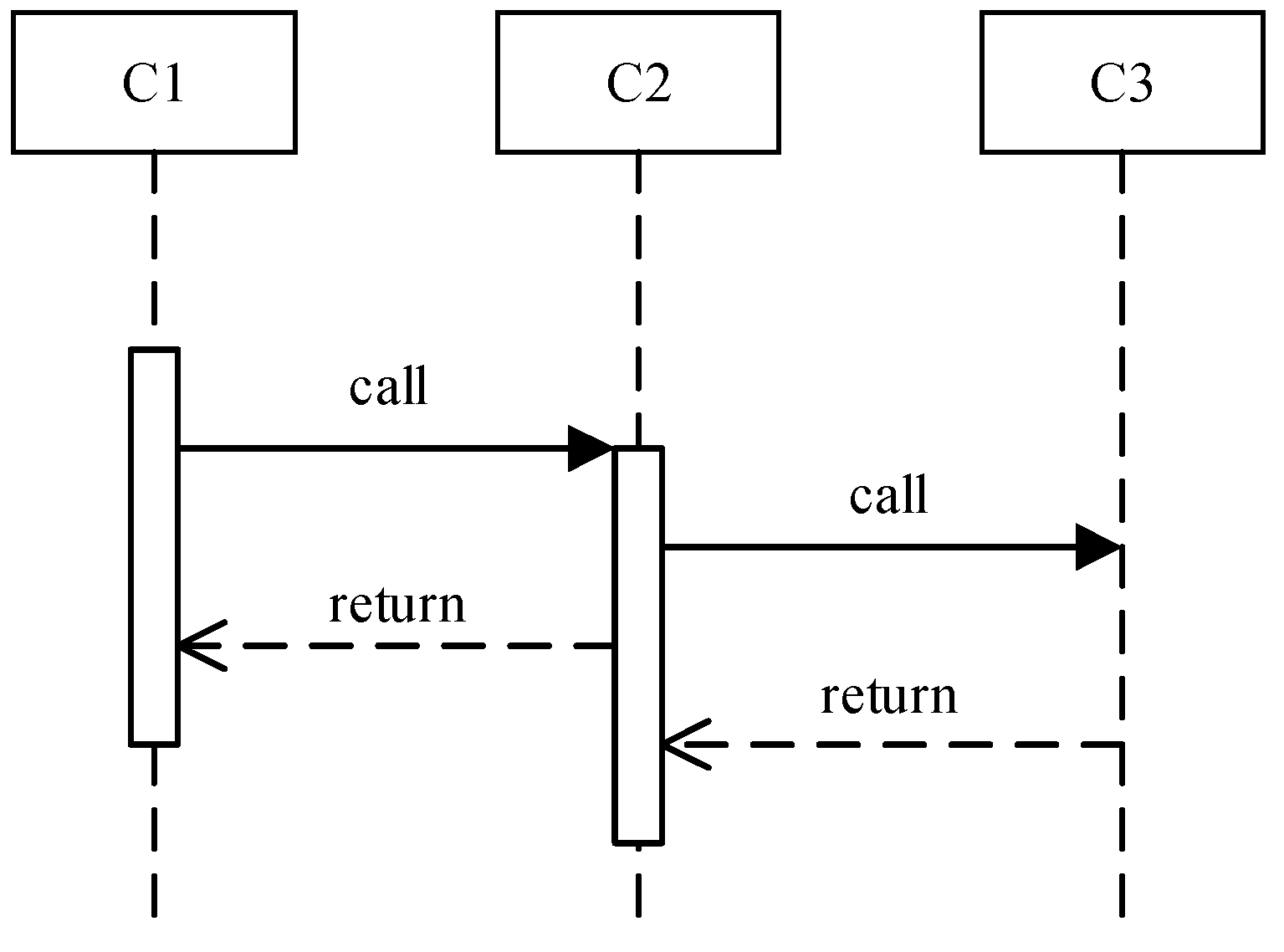
- Transition probability between components under the sequential transition mode
The sequence diagram under the sequential transfer mode is shown in Figure 6. Component C1 initiates a call operation to C2, the message name is ‘call’, and the message type is ‘synchronous’, that is, C1 is in a waiting state after sending a message to C2 and C1 will not perform any other operations or send messages to other components until C2 returns a message. After C1 receives C2′s return message, C1 transfers control authority to C2. Next, C2 initiates a call operation to C3, the message name is ‘call’, and the message type is ‘synchronous’. After C2 sends a message to C3, it is also in a waiting state until C3 returns a message to C2. It can be seen that under the sequential transfer mode, the component that initiates the call transfers control authority to the called component after receiving the return message of the called component, then follows this rule in turn until the transfer mode changes. Under the sequential transfer mode, the operation of each calling component with control authority to initiate a call to the called component can be regarded as a certain event with a probability of 1. In summary, under the sequential transition mode, the transition probability between the RSABM components is 1.
- 2.
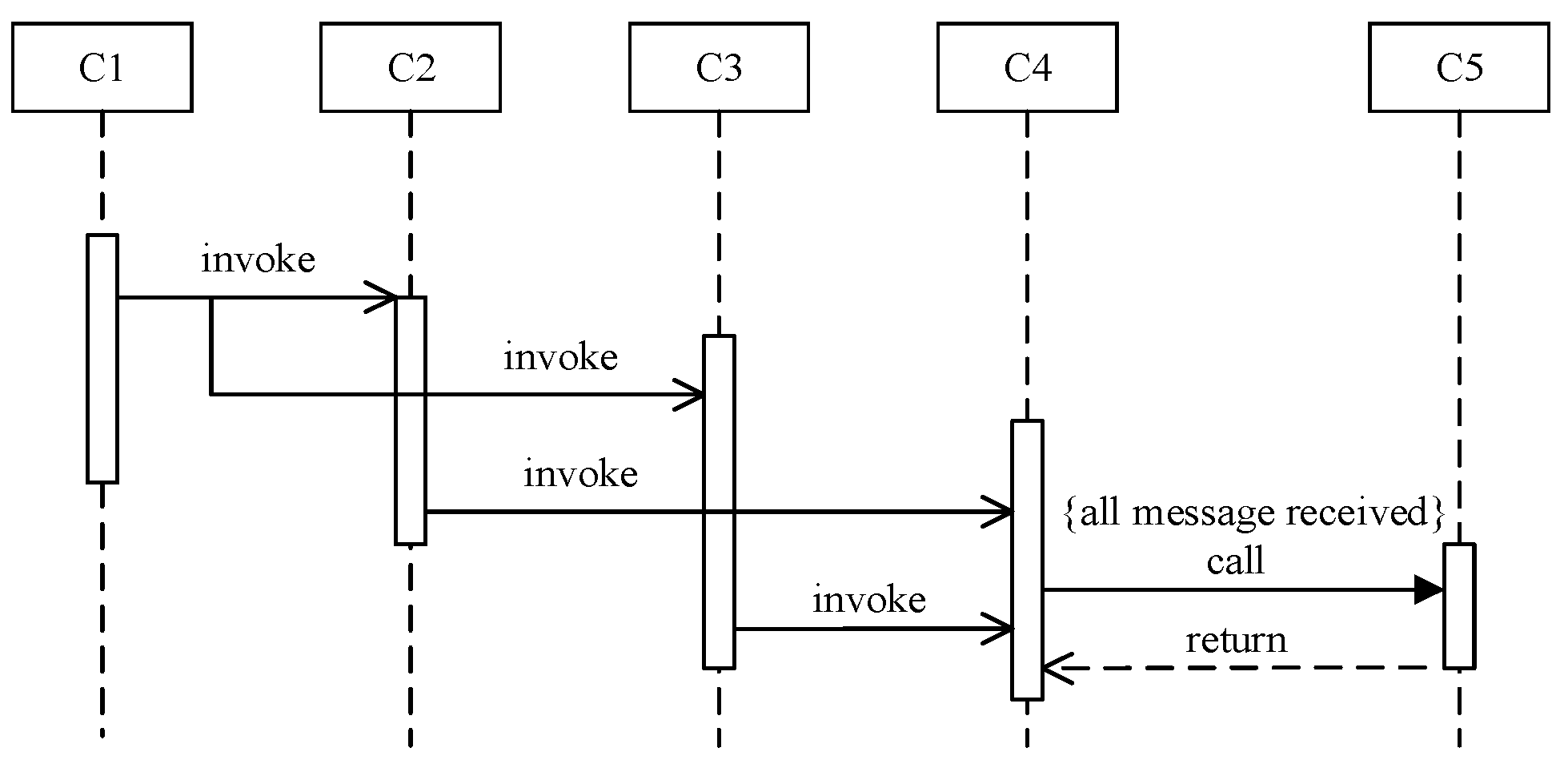
- Transition probability between components under the concurrent transition mode
The sequence diagram under the concurrent transfer mode is shown in Figure 7. Component C1 initiates invocation operations to C2 and C3 at the same time. The message name is ‘invoke’ and the message type is ‘asynchronous’. C2 and C3 are executed concurrently. After the execution is completed, C4 is called, then C4 initiates a synchronous call to C5. The message name is ‘call’ and the message constraint is ‘all messages received’. The constraint indicates that C4 can start execution if and only if C2 and C3 complete their concurrent executions, i.e., only when C2 and C3 executions are completed so the concurrent process is considered to be completed, which means that each concurrent branch must be true, otherwise this relationship will not be established. Based on the above analysis, it can be concluded that under the concurrent transfer mode, the transfer probability between the PRMRE components is 1.
- 3.
- Transition probability between components under the conditional transition mode
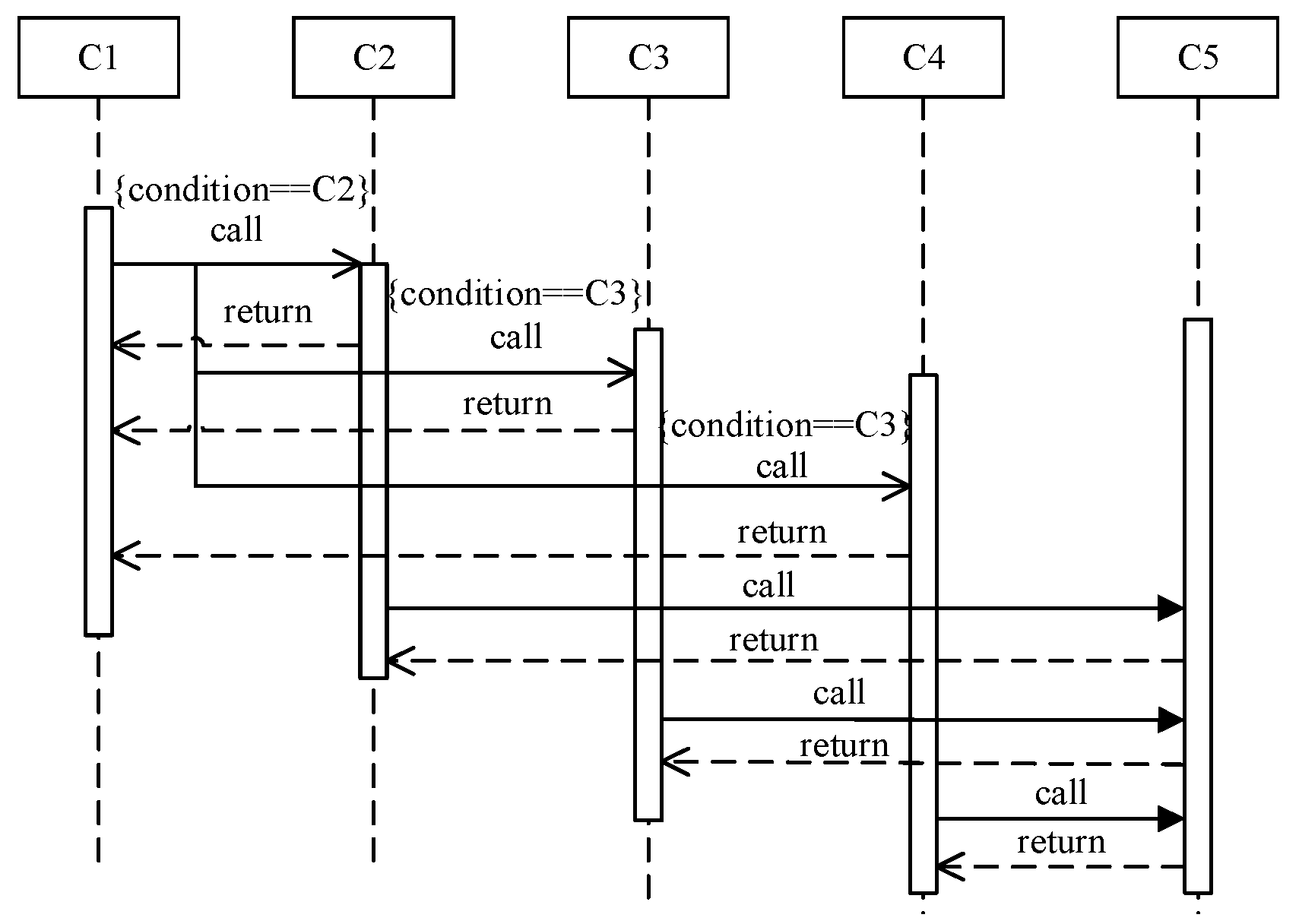
The sequence diagram under the conditional transition mode is shown in Figure 8. Component C1 initiates call operations to C2, C3 and C4 at the same time. The message name is ‘call’, the message type is ‘synchronous’ and the message constraint is {condition = Cn}, where . Among them, the calling operation of C1 is a certain behavior, and the return operations of C2, C3 and C4 to C1 also become certain behaviors under constraints. For example, under the constraint condition {condition = C2}, C1 initiates a call operation to C2, and C2 returns a value to C1. After that, C1 transfers control to C2, and C2 initiates an operation to C5. The message name is ‘call’, the message type is ‘synchronous’, and C5 returns value to C2, then C2 transfers control to C5. So far, the operation of C1 calling C2 under the constraint condition {condition = C2} is completed.
Similarly, the process of C1 calling C3 under constraint {condition = C3} and C1 calling C4 under constraint {condition = C4} can have similar descriptions. Assuming that the occurrence probability of {condition = C2}, {condition = C3} and {condition = C4} are a, b and c, respectively, and a + b + c = 1, then C1 can be considered to move to C2 with the probability of a. To sum up, the transition probability of the component under the conditional transition mode is shown in (1), and the sum of the transition probabilities of all branches is 1:
where represents the number of calls made by Component to , denotes the total number of calls in which has called components under all constraints.
3.2.5. Step 5: Convert PRMRE to a Markov Analysis Model
A Markov analysis model is composed of states and transitions between these states. The states include two types: one is the instantaneous state and the other is the absorption state. The absorption state is then further divided into C and F, where C indicates that the Markov model completes all state transitions and enters the terminal state and F indicates entering the failure state when the state transition occurs. In the process of Markov model state transition, a single state failure can affect the Markov transition behavior. Therefore, the Markov model also needs to describe the reliability of the state and the transition probability between states. Specifically, reliability is expressed by the attributes of the state, and the transition probability between states is represented by the property of state transition.
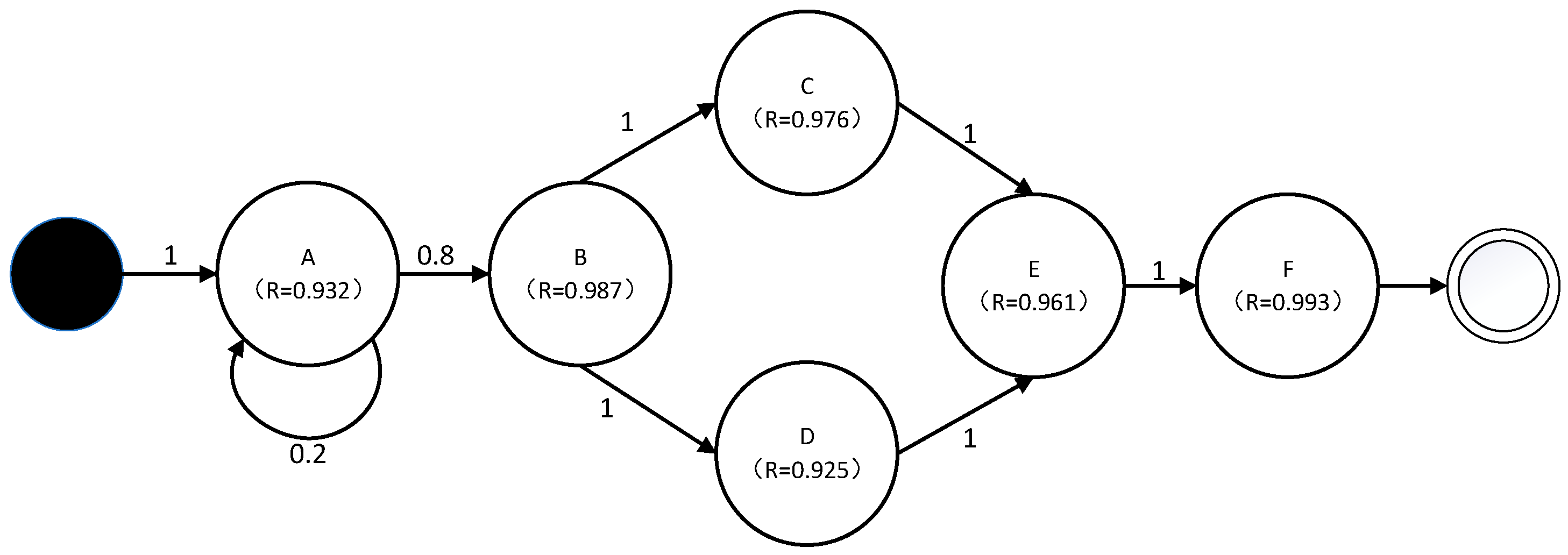
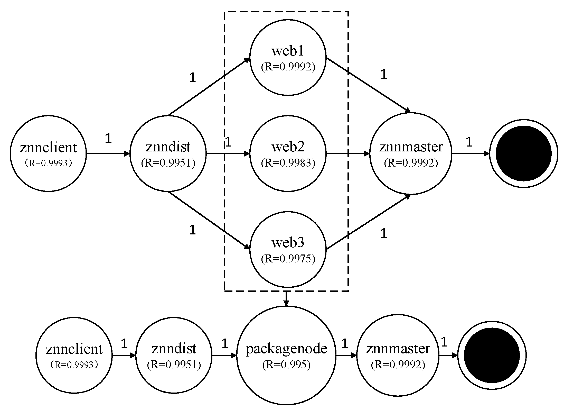
Conversion rules from the PRMRE to the Markov analysis model can be divided into three levels. The first level is the conversion of the model layer, where the source model is PRMRE and the target model is Markov model; the second is the conversion of model components, where the PRMRE component is converted to the state of Markov model; and the last is the conversion of model element tags, where the call between PRMRE components is transformed into the transition between Markov model states. According to the above conversions, the PRMRE shown in Figure 9 can be converted into the Markov analysis model shown in Figure 10.
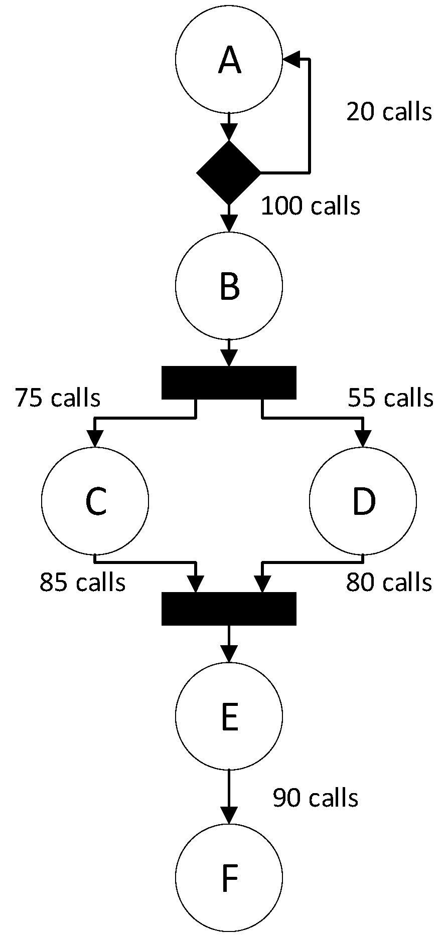
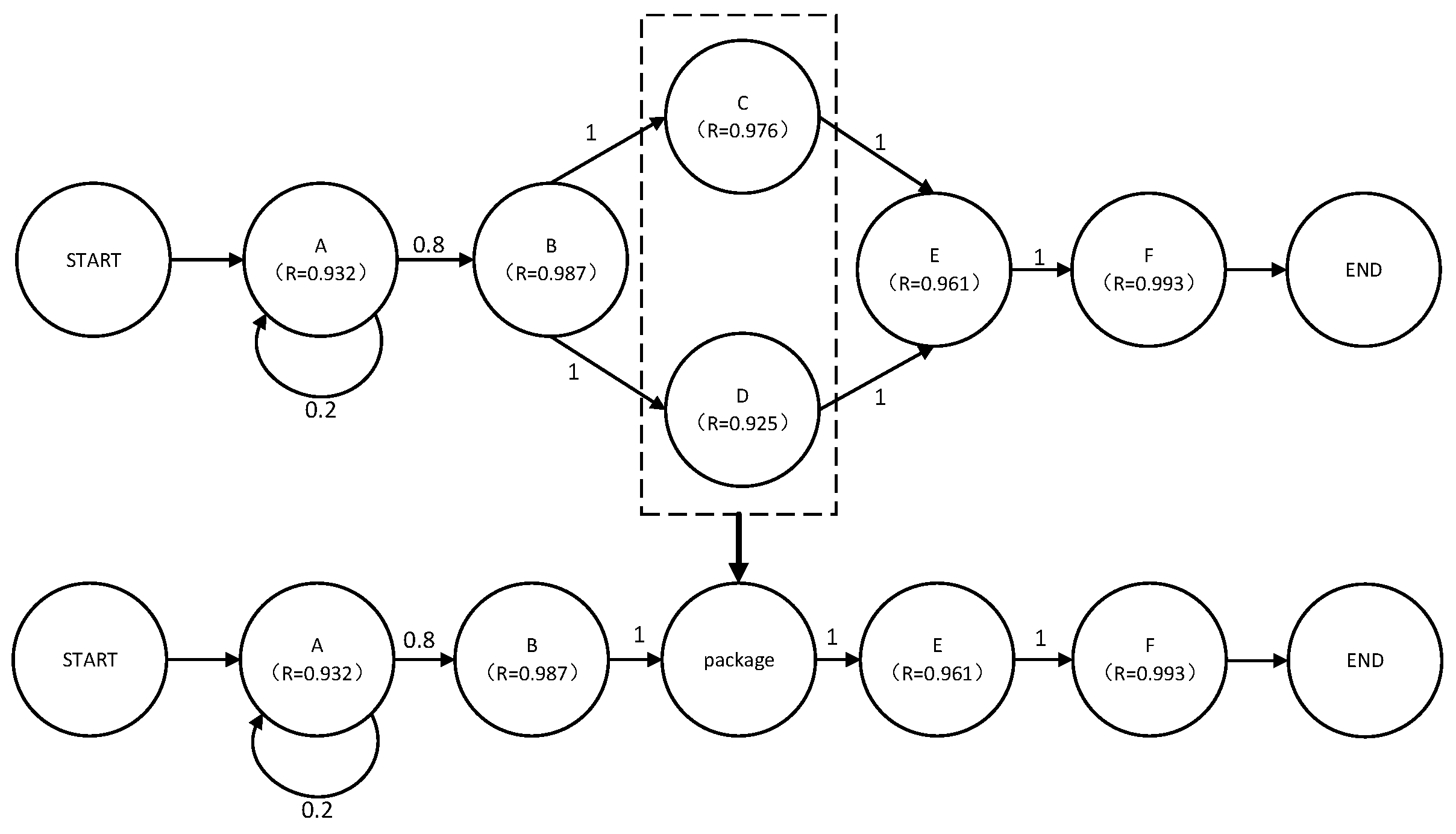
The process of concurrent states in the Markov analysis model is denoted as follows. The components in the PRMRE model may have a concurrent transfer mode, which means that there are concurrent states in the Markov model obtained through model conversion. However, due to the nature of the Markov model, it does not support the concurrent state, and further process is required for the Markov analysis model with concurrent state. A package node is used to solve this problem, where the package node refers to packaging the concurrent states into the Markov analysis model to form an overall state for analysis. As shown in Figure 11, C and D are packaged into one package state for analysis and the overall reliability of the package node needs to be considered. The package node consists of two branches BCE and BDE, so the reliability of the package node is the multiplication of the above two branches, because the transition probability between components in each branch is 1 and each branch definitely occurs, so the reliability of the package node is also equal to the multiplication of the reliability of all components in the node. Specifically, suppose that PRMRE is composed of components where , and there is a concurrent transfer relationship among components, then .
3.2.6. Step 6: Obtain Reliability Prediction
Based on the Markov analysis model, the overall reliability after the execution of different adaptation strategies is predicted, and the adaptation strategy is then selected according to the prediction results. The software in each adaptation stage is composed of components described as , where represents the input component and represents the output component. The state space of the Markov chain can then be represented as , and the transition matrix is defined as follows
where represents the reaching probability from to , represents the reliability of , and the element , that is, indicates the successful arrival probability at from .
Next, the following processing is performed on . Add an absorption state , which means that every component has been called and does not fail, and another absorption state indicates that a failure state occurs when a certain component is called. can only be obtained by the transition of the termination component, where can be obtained by the transition of any component. Therefore, the state space of the Markov model with extended states and can be represented as , and the extension matrix can be constructed as follows:
where the first column indicates the probability of transfers to , for , and the second column indicates the probability of transfers to .
Let denote an by matrix such that
where denotes the identity matrix of size .
Suppose the matrix is the remaining matrix by removing the first column and row of the matrix . The overall system reliability can be computed as follows:
where represents the determinant of the matrix , and the reliability of each component () is considered to be known and can be obtained through empirical data.
Due to limited space, the mathematical background for the above mentioned Markov model can be found in [47].
4. Case Study
4.1. Experimental Setup
Here we use the Znn.com [46] for the case study, which is a popular research object in the field of self-adaptive software and whose adaptation has been realized based on Rainbow framework. Znn.com is built to provide content, both textual and graphical, from back-end databases to clients through a front-end presentation logic within a reasonable response time, while keeping the cost within a certain operating budget. Its goals are, therefore, basically related to performance and cost, without considering reliability change which will be caused by a particular alternative for adaptation action. Therefore, we give a virtual experiment in the context of adaptation, while the result obtained through reliability prediction can give aid in the selection of effective adaptive strategies.
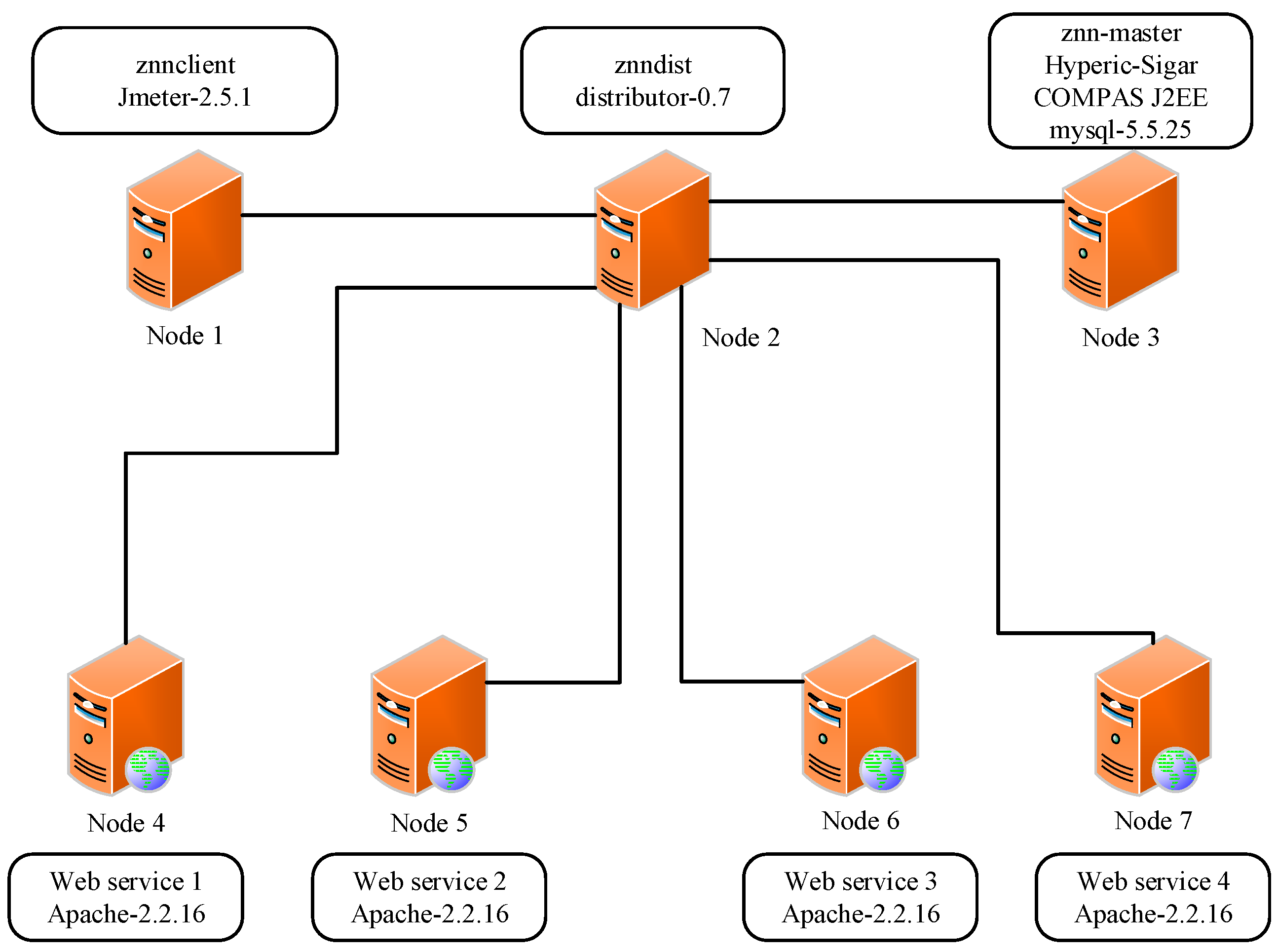
The experimental setup is deployed across seven different machines, shown in Figure 12.
- The web services 1 to 4 are the four content servers running Apache-2.2.16 respectively.
- Znnmaster service (rainbow-znn server) is deployed in Node 3, a separate machine, running Hyperic-sigar, COMPAS J2EE and mysql-5.5.25.
- Znndist is the proxy machine realizing the load balancing service running distributor-0.7 provided by install-lb.sh in the Znn.com installation package.
- Znnclient is deployed in Node 1 running Jmeter-2.5.1 to simulate user access to the Znn.com.
All machines run Ubuntu 19.04 and have 512 MB of memory. It should be noted that the Znn.com is an actual platform running in actual servers and not a simulation model.
4.2. Experiment Procedure
The procedure includes the following steps:
- Step 1:
- Start the Znn.com through the Rainbow and znnmaster console.
- Step 2:
- Activate web service 1 when the system starts running and let other services be in waiting state.
- Step 3:
- Start Jmeter to simulate the user access of the client and write a script for simulating the service request sent by the Znn.com client.
- Step 4:
- Collect the environmental data of Node 3 through the aid of Hyperic-sigar after the system is instantiated.
- Step 5:
- Enter the ‘show-znn.sh-configuration’ command on the console to record the start and end time of each adaptation stage, and the times that the Znn.com has performed adaptation, at which adaptation phase the system enters, while the environmental information of Node 3 is continuously calculated.
- Step 6:
- When the Znn.com enters the fourth adaptation stage, the environmental data collected in the first three adaptation stages should be used to perform the behavior trend analysis of the CPU usage.
- Step 7:
- When the Znn.com enters the fifth adaptation stage, the reliability prediction will be started and the CPU usage behavior trend analysis model obtained in the fourth adaptation stage will be used to analyze the behavior trend of CPU usage during the fifth adaptation stage.
- Step 8:
- We make a copy of the software architecture for each eligible strategy and apply its changes. As previously discussed, at this moment there are three eligible strategies.
- Step 9:
- Generate RMRP for each eligible strategy alternative.
- Step 10:
- Generate PRMRE for each strategy alternative.
- Step 11:
- Generate DTMC for each strategy alternative and calculate the reliability prediction results.
- Step 12:
- Determine the best strategy according to the reliability prediction results.
4.3. Experimental Results
4.3.1. RSABM of the Znn.com
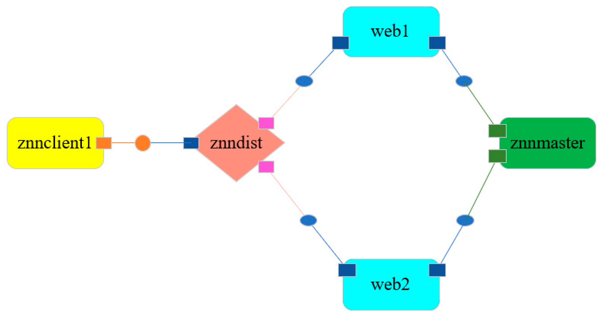
When the Znn.com enters the fifth adaptation stage, the runtime architecture snapshot provided by Rainbow is used to obtain the RSASM, as shown in Figure 13:
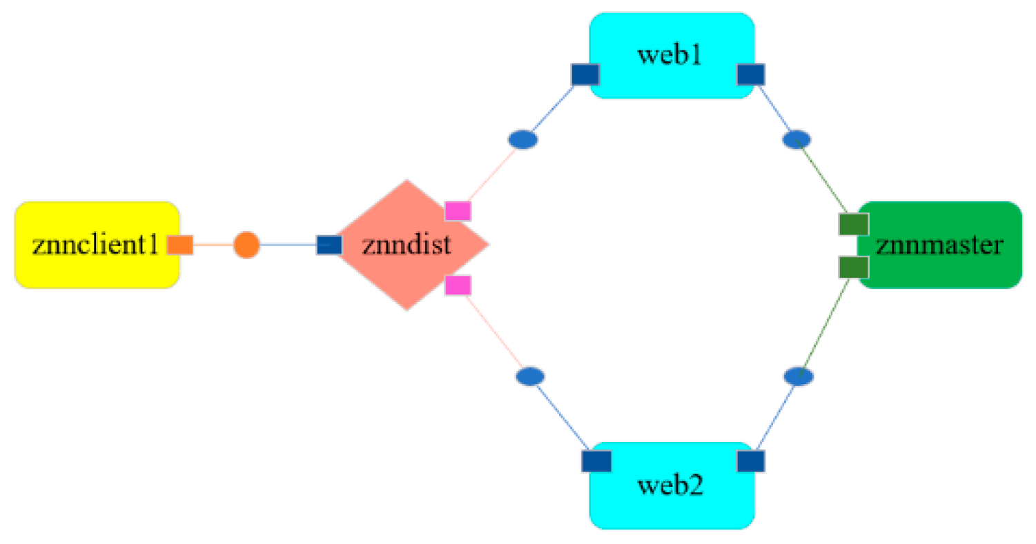
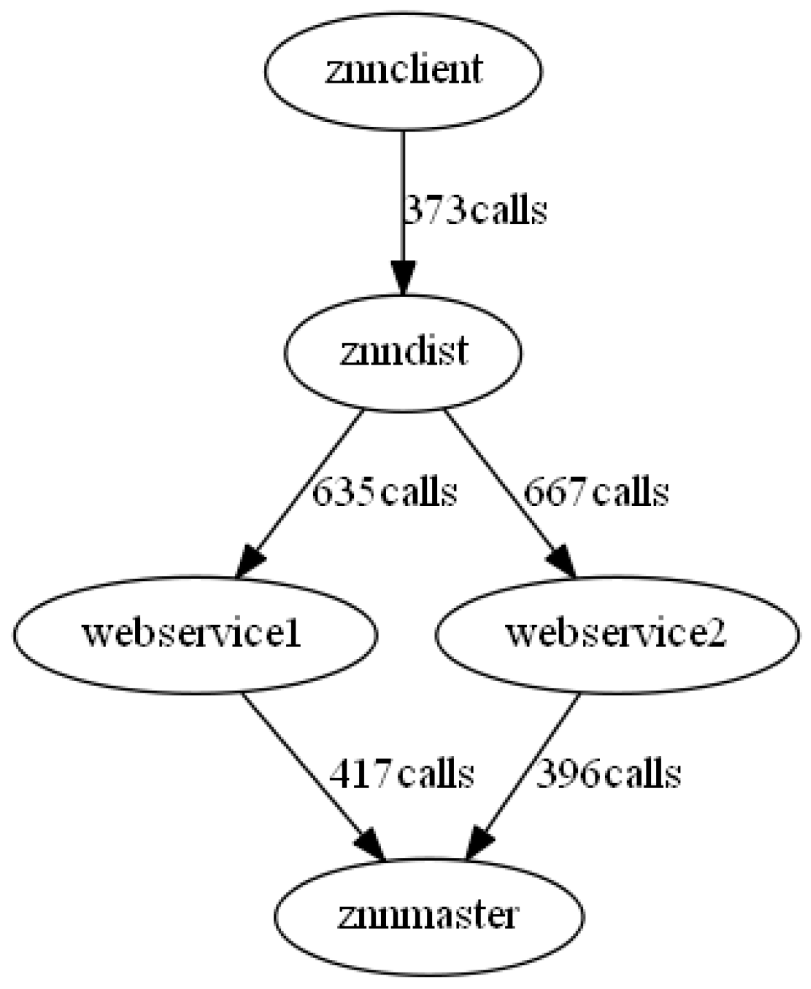
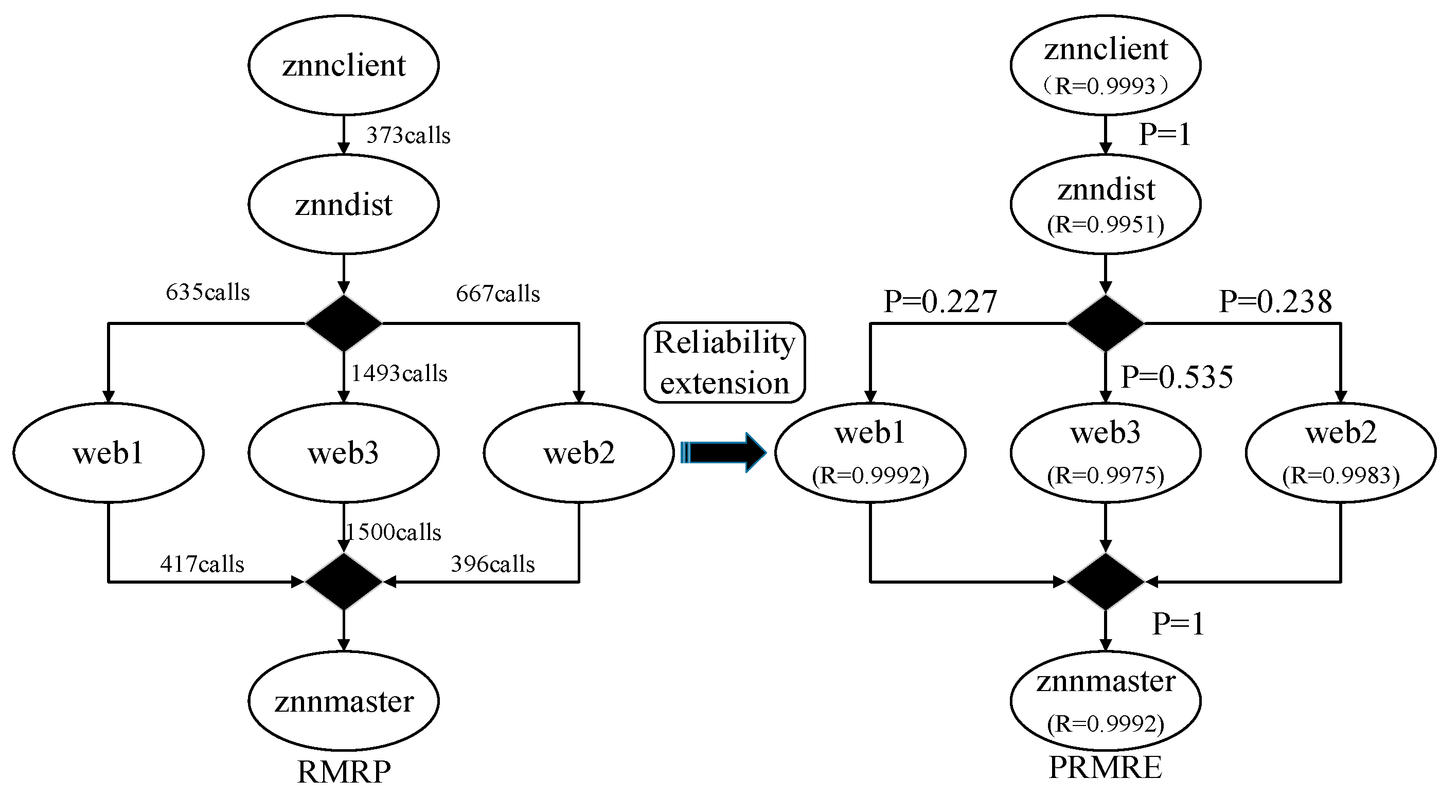
We can determine the objects that need to be monitored, which are znnclientEJB, znndistEJB, webservice1EJB, webservice2EJB and znnmasterEJB. We then use COMPAS software to monitor the above components at runtime. By defining the monitored components in COMPAS, the monitored information is recorded in an ECS.xml file, and the RSABM model of the fifth adaptation stage is generated according to the generation algorithm, which can be seen in Figure 14.
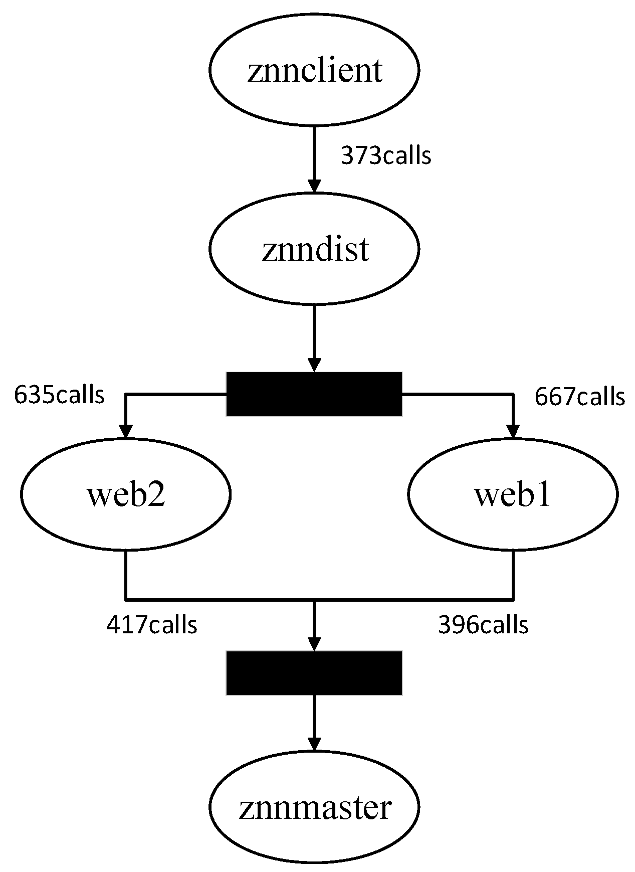
From Figure 14, it can be seen that the component transfer mode has not been marked. Through analysis, it can be known that the load balancing components web1 and web2 can commonly run simultaneously, which means the transition mode of these two components is the concurrent mode. Next, the transfer mode is marked out in Figure 15.
4.3.2. RMRP of the Znn.com
Rainbow-znn provides corresponding adaptive strategies for the CPU usage rate, which is regarded as one of the environment elements of rainbow-znn. According to different CPU usage rate behavior trends, three adaptive strategies may be taken corresponding to the different thresholds.
- Strategy 1:
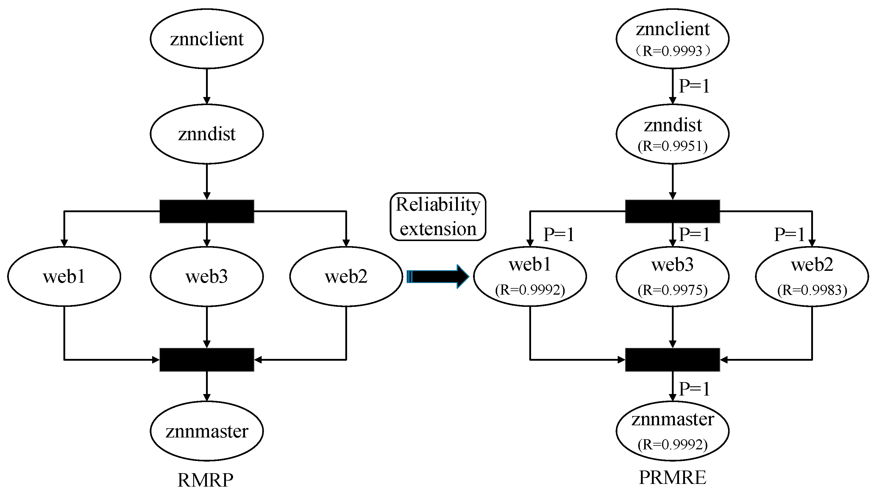
- When the CPU usage rate reaches 80%, an additional server will be added and the schedule mode of the load balancing server will be set to random (supporting concurrency).
- Strategy 2:
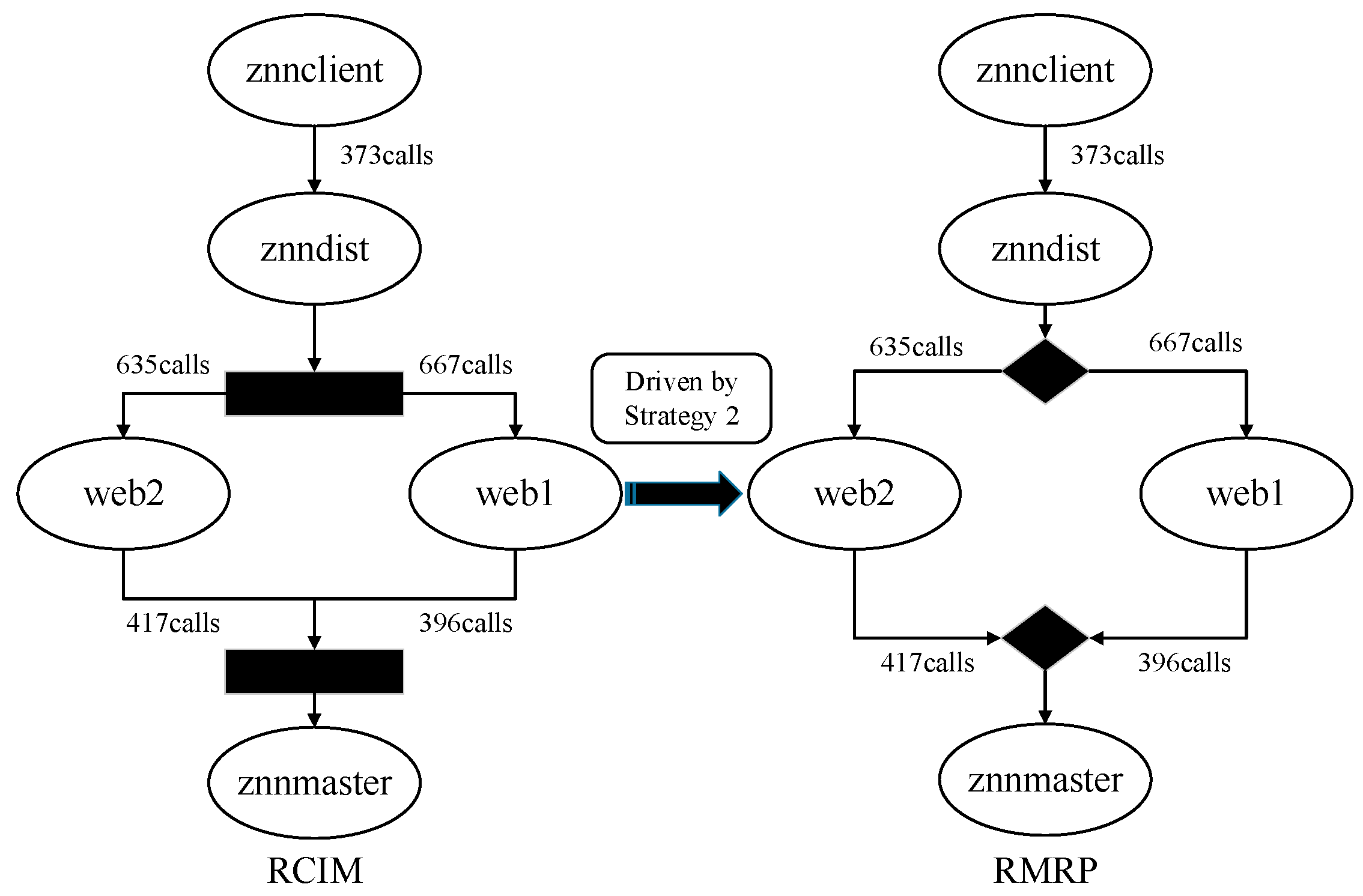
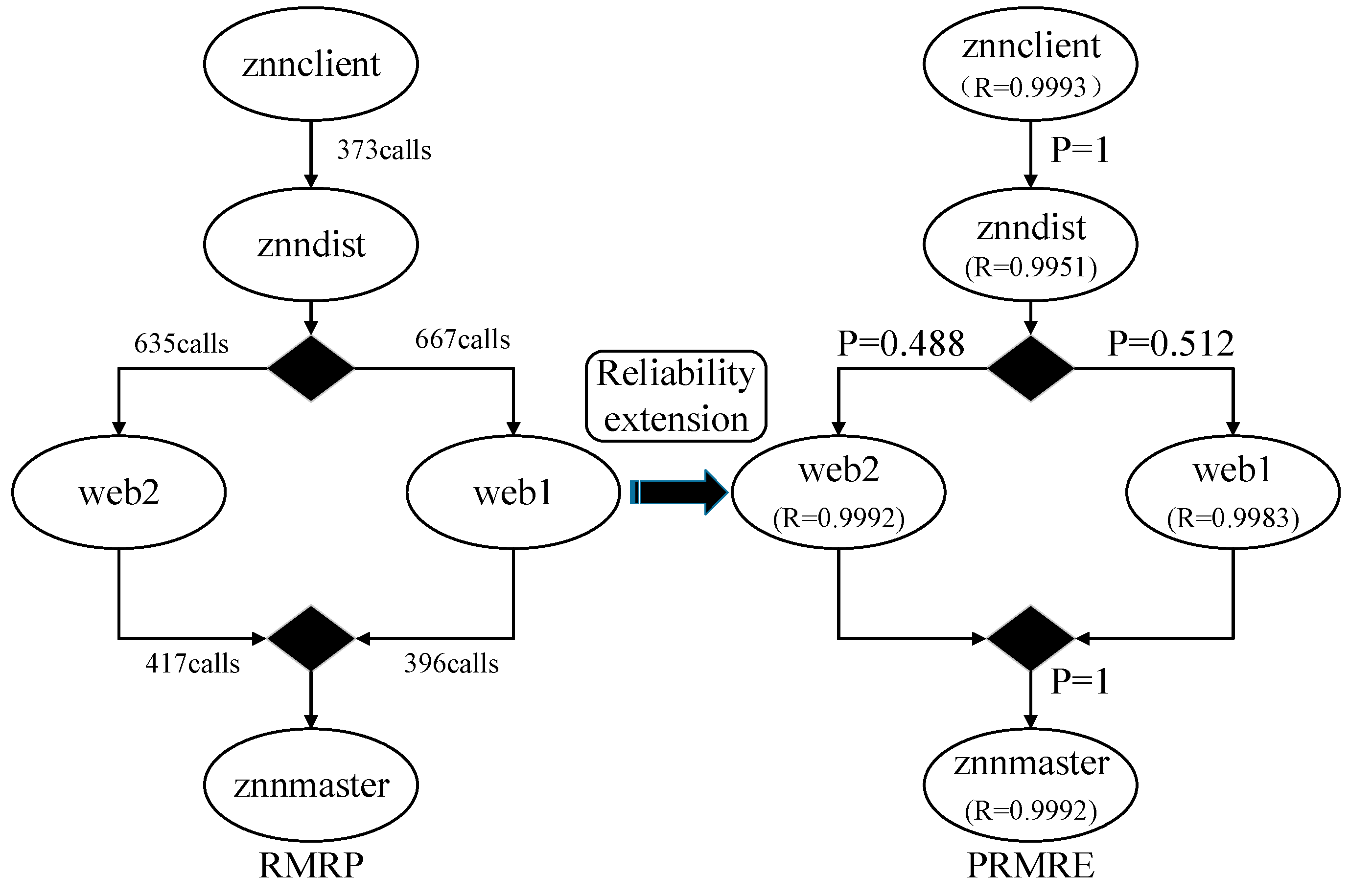
- When the CPU usage rate reaches 80%, switch the news-providing mode from the multimedia mode to the text mode, and set the schedule mode of the load balancing server to the polling mode.
- Strategy 3:
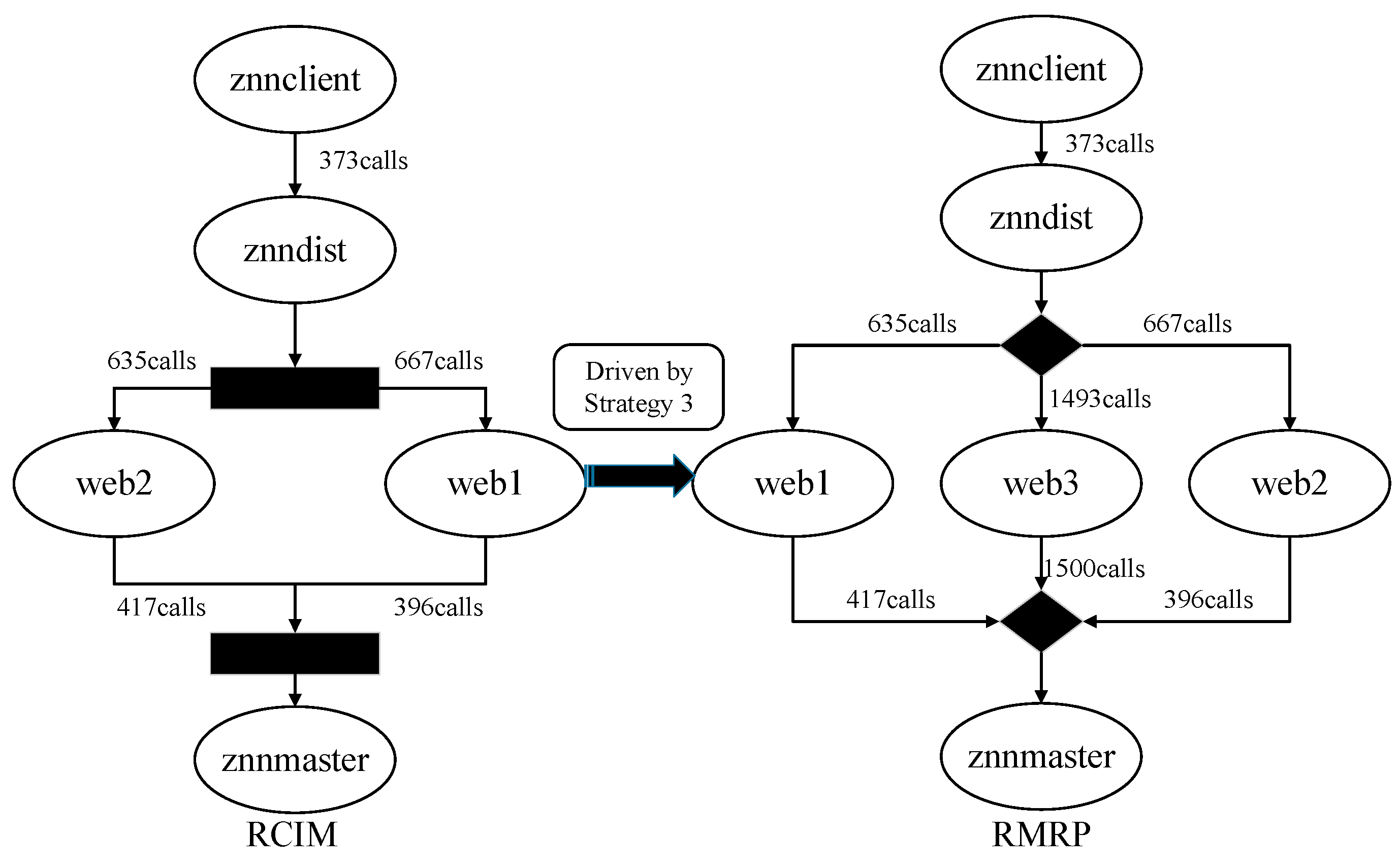
- When the CPU usage rate reaches 80%, add an additional server and set the schedule mode of the load balancing server to the polling mode.
Construct RMRP driven by each strategy accordingly.
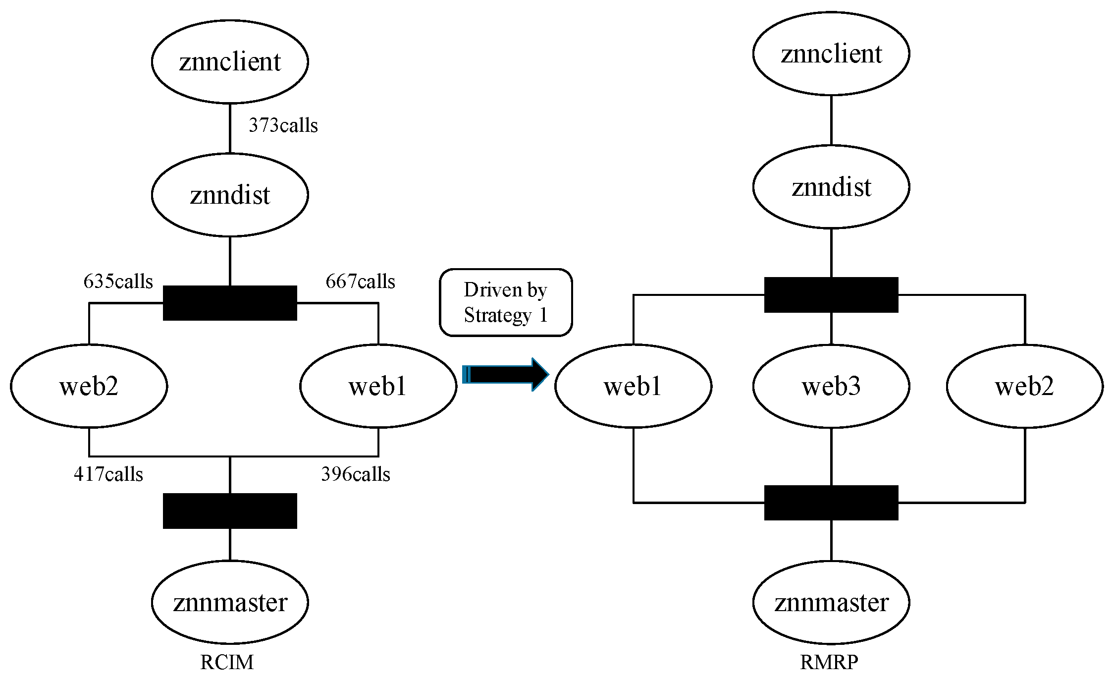
- RMRP driven by Strategy 1
The RMRP driven by Strategy 1 is shown in Figure 16. It should be noted that the relationship between web1 to web3 and znndist after adding a component is still in the concurrent transition mode, so there is no need to speculate the number of calls between these components.
- 2.
- RMRP driven by Strategy 2
Similarly, the RMRP driven by Strategy 2 can be obtained as shown in Figure 17.
The components in the RMRP are all reserved components, so the number of calls between the components can be directly reused.
- 3.
- RMRP driven by Strategy 3
Likewise, the RMRP driven by Strategy 3 can be shown in Figure 18.
Take the LLN of the newly added component as the actual number of calls after the change and determine the number of calls to be 1493 calls.
4.3.3. PRMRE of the Znn.com
Reliability extensions are carried out on RMRPs driven by Strategy 1, Strategy 2 and Strategy 3 respectively.
- Reliability extension on RMRP driven by Strategy 1
This includes adding component reliability and determining the transition probability between components. Since the transition modes in the RMRP only include sequential and concurrent modes, the obtained PRMRE is shown in Figure 19.
- 2.
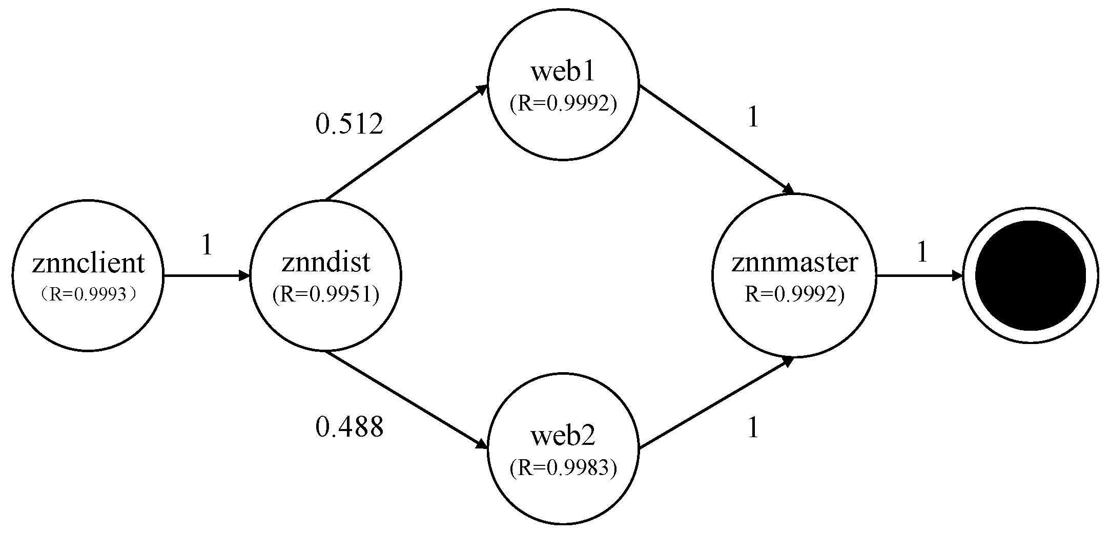
- Reliability extension on RMRP driven by Strategy 2
According to the method of determining the conditional transition probability, the transition probability of RMRP obtained by Strategy 2 can be calculated. Next, the transition probability from znndist to web1 is computed as p = 0.488, and the transition probability from znndist to web2 is p = 0.512. The resulting PRMRE is shown in Figure 20.
- 3.
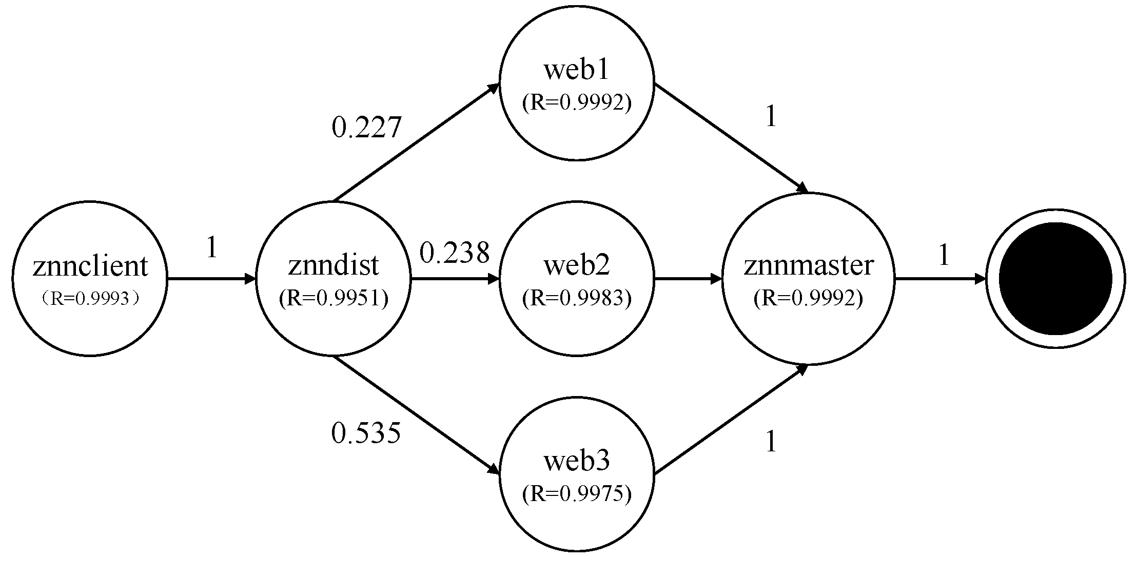
- Reliability extension on RMRP driven by Strategy 3
PRMRE driven by Strategy 3 is shown in Figure 21. Similarly, through the determination method under the conditional transition mode, it can be obtained that the transition probability from znndist to web1 is 0.227, the transition probability from znndist to web2 is 0.535 and the transition probability from znndist to web3 is 0.238.
4.3.4. Analyze the Runtime Reliability Prediction Results Based on Markov Model
Based on the model conversion rules, PRMREs obtained by Strategy 1, Strategy 2 and Strategy 3 are converted into Markov models. These models are shown in Figure 22, Figure 23 and Figure 24, respectively.
Accordingly, the transition matrixes according to Figure 22, Figure 23 and Figure 24 are shown in Table 2, Table 3 and Table 4.
Here the transition matrixes of Markov analysis models after implementing Strategy 1, 2 and 3 are calculated by the software tool Matlab and the final results are shown as follows:
where R1, R2, R3 represent the prediction results of executing Strategy 1 to 3 on the runtime model of the fifth adaptation stage, respectively.
R1 = 0.9886, R2 = 0.9924, R3 = 0.9917
Therefore, the conclusion through this experiment is that after the Znn.com enters the fifth adaptation stage, Strategy 2 should be instantiated before the actual CPU usage reaches 80%.
5. Conclusions and Future Work
The aim of this paper was to study a software reliability prediction method based on RSA rather than DSA. Based on the RSABM obtained through non-intrusive monitoring, the reliability information was expanded to realize the transformation of the Markov analysis model. The software reliability prediction results were then obtained, providing a decision-making basis for the adaptation strategy selection. Our approach encompasses a set of contributions which are summarized as follows:
- Assess the impact of adaptive strategies. This approach presents a method to predict the reliability impact of each adaptive strategy at runtime. We applied the changes imposed by each strategy at the architecture level and predicted the reliability outcome of such changes to support the planning of the self-adaptive system.
- Formal description of the translation from architectural model to DTMC. This method proposed a formal description to a stochastic model. The goal was to support a universal interpretation for the translation.
- Experiment on rainbow-znn software to validate the feasibility of this method.
However, the study still has the following shortcomings:
- The content of the experiment is not sufficient in that the work lacks performance verification and efficiency analysis.
- No sensitivity analysis has been performed on factors which may have an impact on the software reliability prediction results.
Future work needs to supplement and improve the above-mentioned shortcomings in order to improve the completeness of this method and further demonstrate its effectiveness; meanwhile, extended research should be carried out on more types of runtime architecture framework platforms, in addition to the Rainbow framework. How this proposed method can be plugged into the existing environment and realized by automated process remains a research direction.
Author Contributions
Conceptualization, Q.L.; Data curation, Q.L. and T.G.; Funding acquisition, Q.L.; Methodology, Q.L. and T.G.; Project administration, Q.L.; Resources, Q.L.; Software, T.G.; Supervision, Q.L., M.L. and Y.W.; Validation, T.G.; Writing—original draft, Q.L.; Writing—review and editing, Q.L., M.L. and Y.W. All authors have read and agreed to the published version of the manuscript.
Funding
This research was partially funded by “National Key Laboratory of Science and Technology on Reliability and Environmental Engineering of China”, grant number “WDZC2019601A303”.
Institutional Review Board Statement
Not applicable.
Informed Consent Statement
Not applicable.
Data Availability Statement
Not applicable.
Acknowledgments
The authors would like to thank the editor and referees for their valuable comments.
Conflicts of Interest
The authors declare no conflict of interest.
References
- Cheng, B.; de Lemos, R.; Giese, H.; Inverardi, P.; Magee, J.; Andersson, J.; Becker, B.; Bencomo, N.; Brun, Y.; Cukic, B.; et al. Software engineering for self-adaptive systems: A research roadmap. In Lecture Notes in Computer Science; Springer: Berlin/Heidelberg, Germany, 2009; Volume 5525, pp. 1–26. [Google Scholar] [CrossRef] [Green Version]
- Kluge, T. A Role-Based Architecture for Self-Adaptive Cyber-Physical Systems. In Proceedings of the IEEE/ACM 15th International Symposium on Software Engineering for Adaptive and Self-Managing Systems (SEAMS ’20), Seoul, Korea, 7–8 October 2020; ACM: New York, NY, USA, 2020; pp. 1–5. [Google Scholar] [CrossRef]
- Heinrich, R. Architectural run-time models for performance and privacy analysis in dynamic cloud applications. ACM Sigmetrics Perform. Eval. Rev. 2016, 43, 13–22. [Google Scholar] [CrossRef]
- Filieri, A.; Ghezzi, C.; Leva, A.; Maggio, M. Self-adaptive software meets control theory: A preliminary approach supporting reliability requirements. In Proceedings of the IEEE/ACM International Conference on Automated Software Engineering, ACM, Lawrence, KS, USA, 6–10 November 2011; IEEE Computer Society: Los Alamitos, CA, USA; pp. 283–292. [Google Scholar] [CrossRef] [Green Version]
- Angelopoulos, K.; Papadopoulos, A.V.; Souza, V.E.; Mylopoulos, J. Engineering Self-Adaptive Software Systems. ACM Trans. Auton. Adapt. Syst. (TAAS) 2018, 13, 1–27. [Google Scholar] [CrossRef]
- Filieri, A.; Maggio, M.; Angelopoulos, K.; D’ippolito, N.; Gerostathopoulos, I.; Hempel, A.B.; Hoffmann, H.; Jamshidi, P.; Kalyvianaki, E.; Klein, C.; et al. Control Strategies for Self-Adaptive Software Systems. ACM Trans. Auton. Adapt. Syst. 2017, 11, 1–31. [Google Scholar] [CrossRef] [Green Version]
- Kramer, J.; Magee, J. Self-Managed Systems: An Architectural Challenge. In Proceedings of the Future of Software Engineering (FOSE ’07), Minneapolis, MN, USA, 23–25 May 2007. [Google Scholar]
- Chen, B.; Peng, X.; Liu, Y.; Song, S.; Zheng, J.; Zhao, W. Architecture-based behavioral adaptation with generated alternatives and relaxed constraints. IEEE Trans. Serv. Comput. 2019, 12, 73–87. [Google Scholar] [CrossRef]
- Wang, W.-L.; Pan, D.; Chen, M.-H. Architecture-based software reliability modeling. J. Syst. Softw. 2006, 79, 132–146. [Google Scholar] [CrossRef]
- Bass, L.; Clements, P.; Kazman, R. Software Architecture in Practice; Addison-Wesley Longman, Inc.: Upper Saddle River, NJ, USA, 1998. [Google Scholar]
- Medvidovic, N.; Oreizy, P.; Taylor, R.N. Reuse of off-the-shelf components in C2 style architectures. Proceedings of 19th International Conference on Software Engineering, Boston, MA, USA, 17–23 May 1997; pp. 692–700. [Google Scholar]
- Oreizy, P.; Medvidovic, N.; Taylor, R.N. Architecture-based runtime software evolution. In Proceedings of the 20th International Conference on Software Engineering, Kyoto, Japan, 19–25 April 1998; IEEE Computer Society: Los Alamitos, CA, USA, 1998; pp. 177–186. [Google Scholar]
- Blair, G.; Bencomo, N.; France, B. Models@ run.time. Computer 2009, 42, 22–27. [Google Scholar] [CrossRef]
- Heinrich, R.; Jung, R.; Schmieders, E.; Metzger, A.; Hasselbring, W.; Reussner, R.; Pohl, K. Architectural run-time models for operator-in-the-loop adaptation of cloud applications. In Proceedings of the IEEE 9th Symposium on the Maintenance and Evolution of Service-Oriented Systems and Cloud-Based Environments, Bremen, Germany, 2 October 2015. [Google Scholar]
- Huang, G.; Wang, Q.X.; Mei, H.; Yang, F.Q. Research on architecture-based reflective middleware. Ruan Jian Xue Bao/J. Softw. 2003, 14, 1819–1826. (In Chinese) [Google Scholar]
- De Lemos, R.; Giese, H.; Müller, H.A.; Shaw, M.; Andersson, J.; Litoiu, M.; Schmerl, B.; Tamura, G.; Villegas, N.M.; Vogel, T.; et al. Software Engineering for Self-Adaptive Systems: A Second Research Roadmap; Springer: Berlin/Heidelberg, Germany, 2013; pp. 1–32. [Google Scholar]
- Szvetits, M.; Zdun, U. Systematic literature review of the objectives, techniques, kinds, and architectures of models at runtime. Softw. Syst. Model. 2016, 15, 31–69. [Google Scholar] [CrossRef]
- Lehmann, G.; Blumendorf, M.; Trollmann, F.; Albayrak, S. Meta-modeling runtime models. In Proceedings of the 2010 International Conference on Models in Software Engineering, Oslo, Norway, 3 October 2010; Springer: Berlin/Heidelberg, Germany, 2010; pp. 209–223. [Google Scholar]
- Bencomo, N.; France, R.; Cheng, B.; Aßmann, U. [email protected]: Foundations, Applications, and Roadmaps. In Lecture Notes in Computer Science; Springer: Berlin/Heidelberg, Germany, 2014; Volume 8378, pp. 1–318. [Google Scholar]
- Song, H.; Huang, G.; Wu, Y.; Chauvel, F.; Sun, Y.; Shao, W.; Mei, H. Modeling and maintaining runtime software architectures. Ruan Jian Xue Bao/J. Softw. 2013, 24, 1731–1745. (In Chinese) [Google Scholar] [CrossRef]
- Garlan, D.; Cheng, S.W.; Huang, A.C.; Schmerl, B.; Steenkiste, P. Rainbow: Architecture-based self-adaptation with reusable infrastructure. Computer 2004, 37, 46–54. [Google Scholar] [CrossRef]
- Floch, J.; Hallsteinsen, S.; Stav, E.; Eliassen, F.; Lund, K.; Gjorven, E. Using Architecture Models for Runtime Adaptability. IEEE Softw. 2006, 23, 62–70. [Google Scholar] [CrossRef]
- Hong, M.; Gang, H. PKUAS: An architecture-based reflective component operating platform. In Proceedings of the IEEE International Workshop on Distributed Computing Systems, Suzhou, China, 26–28 May 2004; IEEE Computer Society: Los Alamitos, CA, USA, 2004. [Google Scholar]
- Morin, B.; Barais, O.; Nain, G.; Jezequel, J.-M. Taming dynamically adaptive systems using models and aspects. In Proceedings of the 2009 IEEE 31st International Conference on Software Engineering, Vancouver, BC, Canada, 16–24 May 2009; pp. 122–132. [Google Scholar]
- Elkhodary, A.; Esfahani, N.; Malek, S. FUSION: A framework for engineering self-tuning self-adaptive software systems. In Proceedings of the Eighteenth ACM SIGSOFT International Symposium on Foundations of Software Engineering, Santa Fe, NM, USA, 7–11 November 2010; pp. 7–16. [Google Scholar]
- D’Ippolito, N.; Braberman, V.; Kramer, J.; Magee, J.; Sykes, D.; Uchitel, S. Hope for the best, prepare for the worst: Multi-tier control for adaptive systems. In Proceedings of the 36th International Conference on Software Engineering, Hyderabad, India, 31 May–7 June 2014; pp. 688–699. [Google Scholar]
- Chen, B.; Peng, X.; Yu, Y.; Nuseibeh, B.; Zhao, W. Self-adaptation through incremental generative model transformations at runtime. In Proceedings of the 36th International Conference on Software Engineering, Hyderabad, India, 31 May–7 June 2014; pp. 676–687. [Google Scholar]
- Zhu, Y.; Huang, G.; Mei, H. Quality Attribute Scenario Based Architectural Modeling for Self-Adaptation Supported by Architecture-based Reflective Middleware. In Proceedings of the 11th Asia-Pacific Software Engineering Conference, Busan, Korea, 30 November–3 December 2004. [Google Scholar]
- Calinescu, R.; Ghezzi, C.; Kwiatkowska, M.; Mirandola, R. Self-Adaptive Software Needs Quantitative Verification at Runtime. Commun. ACM 2012, 55, 69–77. [Google Scholar] [CrossRef]
- Calinescu, R.; Weyns, D.; Gerasimou, S.; Iftikhar, M.U.; Habli, I.; Kelly, T. Engineering Trustworthy Self-Adaptive Software with Dynamic Assurance Cases. IEEE Trans. Softw. Eng. 2017, 44, 1039–1069. [Google Scholar] [CrossRef] [Green Version]
- Yang, J.; Zhang, J. Combinatorial Testing: Principles and Methods. J. Softw. 2009, 20, 1393–1405. (In Chinese) [Google Scholar]
- Loukil, S.; Kallel, S.; Jmaiel, M. An approach based on runtime models for developing dynamically adaptive systems. Future Gener. Comput. Syst. 2016, 68, 365–375. [Google Scholar] [CrossRef]
- Chen, L. Design and Implementation of Strategy-Driven Adaptive Software Simulation Platform; Peking University: Beijing, China, 2014. (In Chinese) [Google Scholar]
- Perez-Palacin, D.; Mirandola, R.; Merseguer, J. QoS and energy management with Petrinets: A self-adaptive framework. J. Syst. Softw. 2012, 85, 2796–2811. [Google Scholar] [CrossRef] [Green Version]
- Franks, G.; Al-Omari, T.; Woodside, M.; Das, O.; Derisavi, S. Enhanced modeling and solution of layered queueing networks. IEEE Trans. Softw. Eng. 2009, 35, 148–161. [Google Scholar] [CrossRef]
- Sato, N.; Trivedi, K.S. Stochastic modeling of composite web services for closed-form analysis of their performance and reliability bottlenecks. In Lecture Notes in Computer Science; Springer: Berlin/Heidelberg, Germany, 2007; Volume 4749, pp. 107–118. [Google Scholar]
- Hessel, A.; Larsen, K.G.; Mikucionis, M.; Nielsen, B.; Pettersson, P.; Skou, A. Testing real-time systems using UPPAAL. In Formal Methods and Testing: An Outcome of the FORTEST Network; Hierons, R.M., Bowen, J.P., Harman, M., Eds.; Springer: Berlin/Heidelberg, Germany, 2008; pp. 77–117. [Google Scholar] [CrossRef]
- Kwiatkowska, M.; Norman, G.; Parker, D. PRISM 4.0: Verification of probabilistic real-time systems. In Lecture Notes in Computer Science; Springer: Berlin/Heidelberg, Germany, 2011; Volume 6806, pp. 585–591. [Google Scholar]
- Behrmann, G.; David, A.; Larsen, K.G.; Hakansson, J.; Petterson, P.; Yi, W.; Hendriks, M. UPPAAL 4.0. In Proceedings of the 3rd International Conference on Quantitative Evaluation Systems, Riverside, CA, USA, 11–14 September 2006; pp. 125–126. [Google Scholar] [CrossRef]
- Filieri, A.; Ghezzi, C.; Tamburrelli, G. A formal approach to adaptive software: Continuous assurance of non-functional requirements. Formal Aspects Comput. 2012, 24, 163–186. [Google Scholar] [CrossRef] [Green Version]
- Filieri, A.; Tamburrelli, G.; Ghezzi, C. Supporting Self-Adaptation via Quantitative Verification and Sensitivity Analysis at Run Time. IEEE Trans. Softw. Eng. 2016, 42, 75–99. [Google Scholar] [CrossRef]
- Calinescu, R.; Kwiatkowska, M. Using quantitative analysis to implement autonomic it systems. In Proceedings of the 2009 IEEE 31st International Conference on Software Engineering, Vancouver, BC, Canada, 16–24 May 2009; pp. 100–110. [Google Scholar]
- Calinescu, R.; Grunske, L.; Kwiatkowska, M.; Mirandola, R.; Tamburrelli, G. Dynamic QoS management and optimization in service-based systems. IEEE Trans. Softw. Eng. 2011, 37, 387–409. [Google Scholar] [CrossRef]
- Ghezzi, C.; Pinto, L.S.; Spoletini, P.; Tamburrelli, G. Managing non-functional uncertainty via model-driven adaptivity. In Proceedings of the 2013 35th International Conference on Software Engineering (ICSE), San Francisco, CA, USA, 18–26 May 2013; pp. 33–42. [Google Scholar]
- Moreno, G.A.; Càmara, J.; Garlan, D.; Schmerl, B. Proactive self-adaptation under uncertainty: A probabilistic model checking approach. In Proceedings of the 2015 10th Joint Meeting on Foundations of Software Engineering, El Paso, TX, USA, 30 August 2015; pp. 1–12. [Google Scholar]
- Cheng, S.W. Rainbow: Cost-Effective Software Architecture-Based Self-Adaptation; Carnegie Mellon University: Schenley Park Pittsburgh, PA, USA, 2016. [Google Scholar]
- Cheung, R.C. A User-Oriented Software Reliability Model. IEEE Trans. Softw. Eng. 1980, SE-6, 118–125. [Google Scholar] [CrossRef]
Figure 1.
Timing of runtime reliability prediction method’s application.

Figure 2.
Schema of self-adaptive runtime reliability prediction method.

Figure 3.
Snapshot for runtime architecture of rainbow-znn.

Figure 4.
Schema of RMRP.

Figure 5.
Change rules for different transfer modes under different operations: (a) The change rule for the sequential transfer mode under adding a component operation; (b) The change rule for the conditional transfer mode under adding a component operation; (c) The change rule for the concurrent transfer mode under adding a component operation; (d) The change rule for the conditional transfer mode under deleting a component operation; (e) The change rule for the concurrent transfer mode under deleting a component operation; (f) The change rule for the conditional transfer mode under replacing a component operation; (g) The change rule for the concurrent transfer mode under replacing a component operation; (h) The change rule for the concurrent transfer mode under the operation of changing the message calling mode; (i) The change rule for the conditional transfer mode under the operation of changing the message calling mode.

Figure 6.
Sequence diagram under the sequential transition mode.

Figure 7.
Sequence diagram under the concurrent transition mode.

Figure 8.
Sequence diagram under the conditional transition mode.

Figure 9.
Runtime reliability extension model for prediction.

Figure 10.
Markov analysis model.

Figure 11.
An example of concurrent state process in the Markov model.

Figure 12.
Deployment of experimental environment.

Figure 13.
Runtime architecture snapshot of rainbow-znn.

Figure 14.
RSABM of the Znn.com system without annotated transfer mode in the fifth adaptation stage.
Figure 14.
RSABM of the Znn.com system without annotated transfer mode in the fifth adaptation stage.

Figure 15.
RSABM of the Znn.com in the fifth adaptation stage.

Figure 16.
RMRP driven by Strategy 1.

Figure 17.
RMRP driven by Strategy 2.

Figure 18.
RMRP driven by Strategy 3.

Figure 19.
PRMRE driven by Strategy 1.

Figure 20.
PRMRE driven by Strategy 2.

Figure 21.
PRMRE driven by Strategy 3.

Figure 22.
Markov analysis model after Strategy 1.

Figure 23.
Markov analysis model after Strategy 2.

Figure 24.
Markov analysis model after Strategy 3.


Table 1.
Runtime component transition modes.
| Transition Mode | Graphical Description |
|---|---|
| Sequential transition |  |
| Conditional transition |  |
| Concurrent transition |  |
Table 2.
The transition matrix after implementing Strategy 1.
| Znnclient | Znndist | Packagenode | Znnmaster | End | Fail | |
|---|---|---|---|---|---|---|
| znnclient | 0 | 0.9993 | 0 | 0 | 0 | 0.0007 |
| znndist | 0 | 0 | 0.9951 | 0 | 0 | 0.0049 |
| packagenode | 0 | 0 | 0 | 0.995 | 0 | 0.005 |
| znndb | 0 | 0 | 0 | 0 | 0.9992 | 0.0008 |
| end | 0 | 0 | 0 | 0 | 1 | 0 |
| fail | 0 | 0 | 0 | 0 | 0 | 1 |
Table 3.
The transition matrix after implementing Strategy 2.
| Znnclient | Znndist | Web1 | Web2 | Znnmaster | End | Fail | |
|---|---|---|---|---|---|---|---|
| znnclient | 0 | 0.9993 | 0 | 0 | 0 | 0 | 0.0007 |
| znndist | 0 | 0 | 0.5095 | 0.4856 | 0 | 0 | 0.0049 |
| web1 | 0 | 0 | 0 | 0 | 0.9992 | 0 | 0.0008 |
| web2 | 0 | 0 | 0 | 0 | 0.9983 | 0 | 0.0017 |
| znndb | 0 | 0 | 0 | 0 | 0 | 0.9992 | 0.0008 |
| end | 0 | 0 | 0 | 0 | 0 | 0 | 0 |
| fail | 0 | 0 | 0 | 0 | 0 | 0 | 0 |
Table 4.
The transition matrix after implementing Strategy 3.
| Znnclient | Znndist | Web1 | Web2 | Web3 | Znnmaster | End | Fail | |
|---|---|---|---|---|---|---|---|---|
| znnclient | 0 | 0.9993 | 0 | 0 | 0 | 0 | 0 | 0.0007 |
| znndist | 0 | 0 | 0.2259 | 0.2368 | 0.5324 | 0 | 0 | 0.0049 |
| web1 | 0 | 0 | 0 | 0 | 0 | 0.9992 | 0 | 0.0008 |
| web2 | 0 | 0 | 0 | 0 | 0 | 0.9983 | 0 | 0.0017 |
| web3 | 0 | 0 | 0 | 0 | 0 | 0.9975 | 0 | 0.0025 |
| znndb | 0 | 0 | 0 | 0 | 0 | 0 | 0.9992 | 0.0008 |
| end | 0 | 0 | 0 | 0 | 0 | 0 | 0 | 0 |
| fail | 0 | 0 | 0 | 0 | 0 | 0 | 0 | 0 |
Publisher’s Note: MDPI stays neutral with regard to jurisdictional claims in published maps and institutional affiliations. |
© 2022 by the authors. Licensee MDPI, Basel, Switzerland. This article is an open access article distributed under the terms and conditions of the Creative Commons Attribution (CC BY) license (https://creativecommons.org/licenses/by/4.0/).
Share and Cite
MDPI and ACS Style
Li, Q.; Lu, M.; Gu, T.; Wu, Y. Runtime Software Architecture-Based Reliability Prediction for Self-Adaptive Systems. Symmetry 2022, 14, 589. https://doi.org/10.3390/sym14030589
AMA Style
Li Q, Lu M, Gu T, Wu Y. Runtime Software Architecture-Based Reliability Prediction for Self-Adaptive Systems. Symmetry. 2022; 14(3):589. https://doi.org/10.3390/sym14030589
Chicago/Turabian StyleLi, Qiuying, Minyan Lu, Tingyang Gu, and Yumei Wu. 2022. "Runtime Software Architecture-Based Reliability Prediction for Self-Adaptive Systems" Symmetry 14, no. 3: 589. https://doi.org/10.3390/sym14030589
Note that from the first issue of 2016, this journal uses article numbers instead of page numbers. See further details here.