
On the Performance of a Nonlinear Position-Velocity Controller to Stabilize Rotor-Active Magnetic-Bearings System


 , and
, and 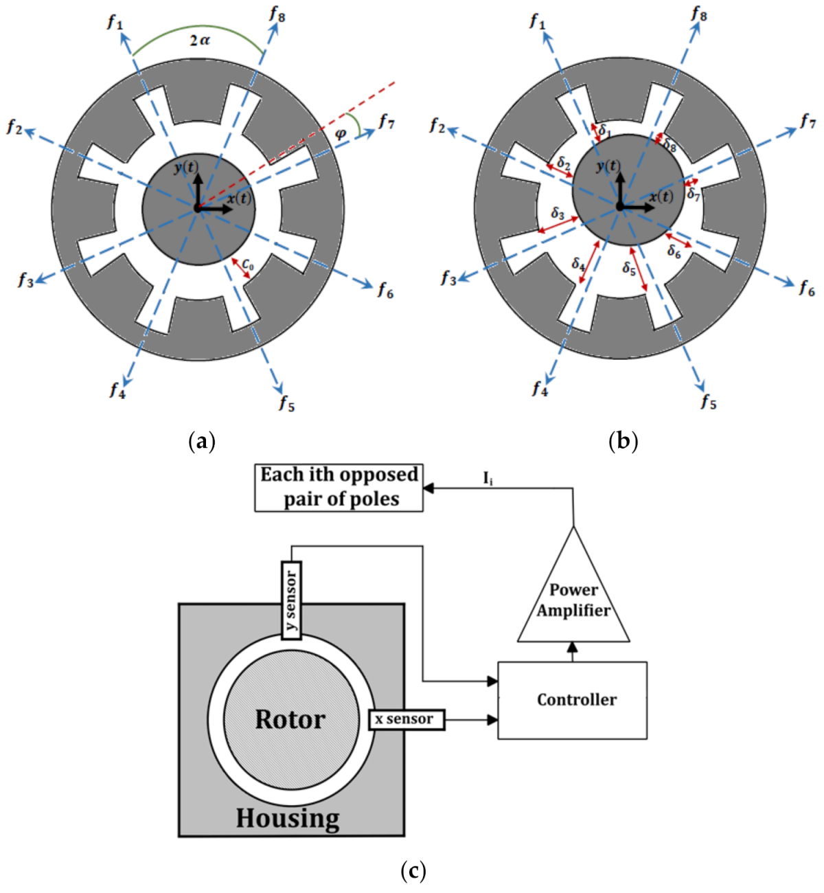
Abstract
:1. Introduction
2. Mathematical Modelling
3. System Periodic Solution and Slow-Flow Modulating Equations
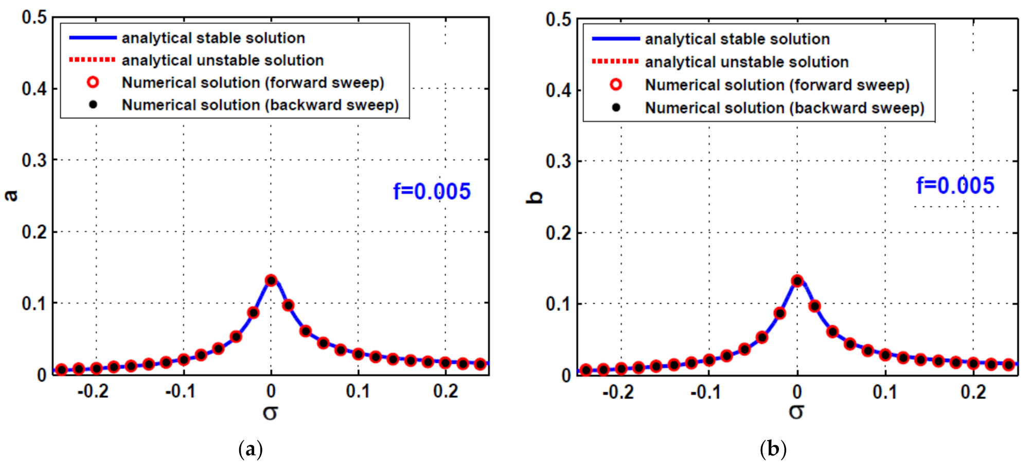
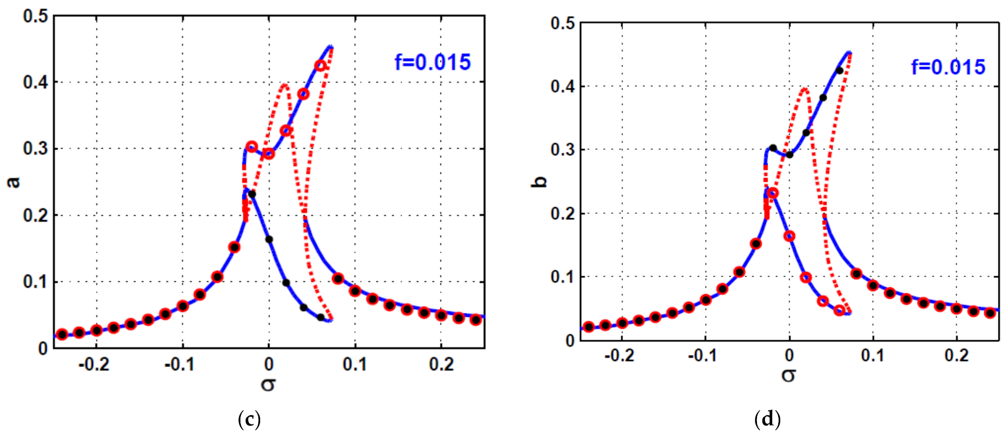
4. Sensitivity Investigations
4.1. Sensitivity Analysis of Linear Position-Velocity Controller ( and )
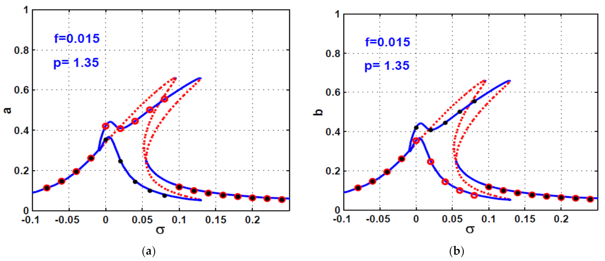
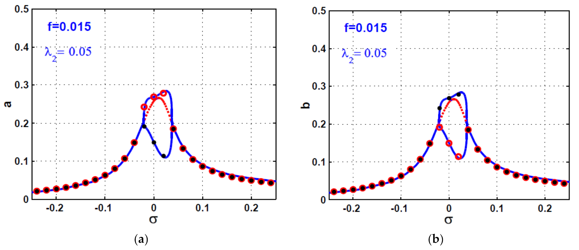
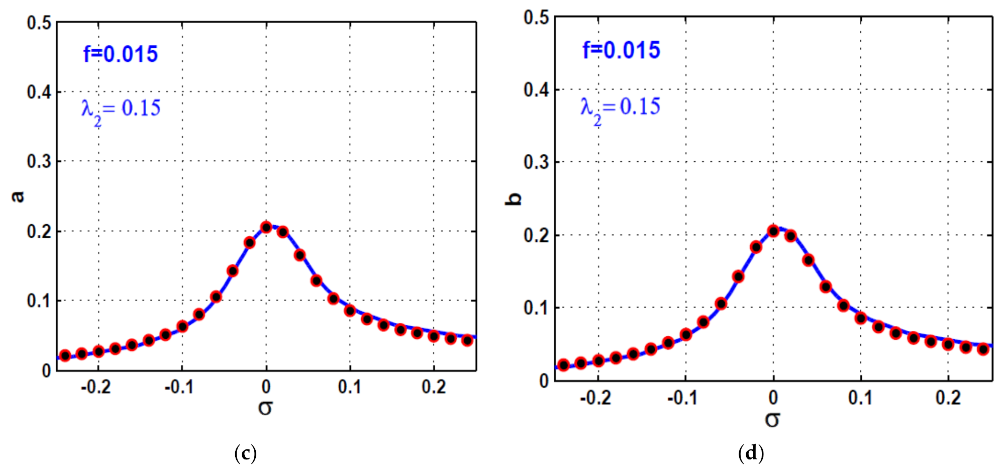
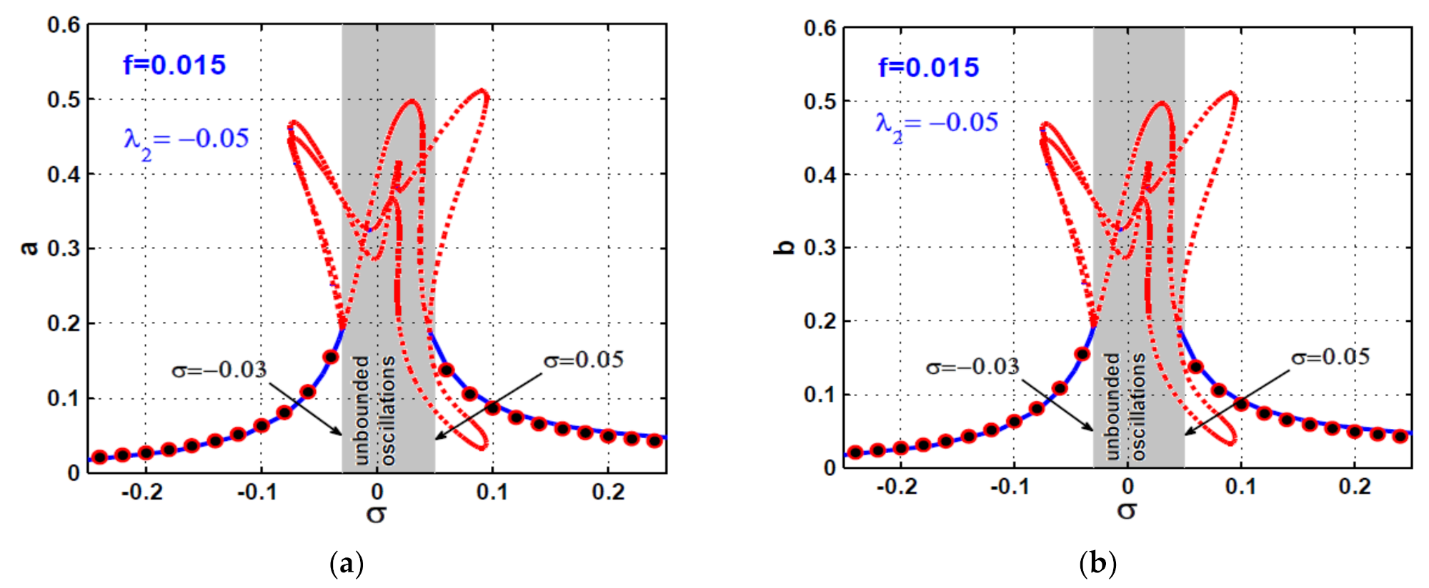
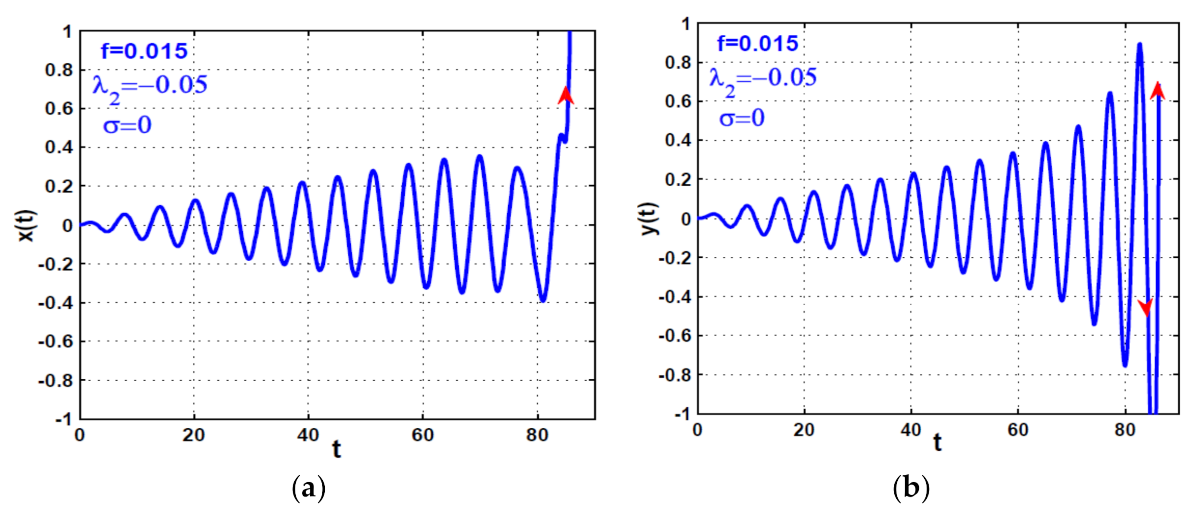
4.2. Sensitivity Analysis of Nonlinear Position-Velocity Controller ( and )
5. Conclusions
- Optimal linear position gain should be as small as possible; however, it should be greater than (i.e., gain ) to guarantee system stability by making system natural frequency always have a positive value.
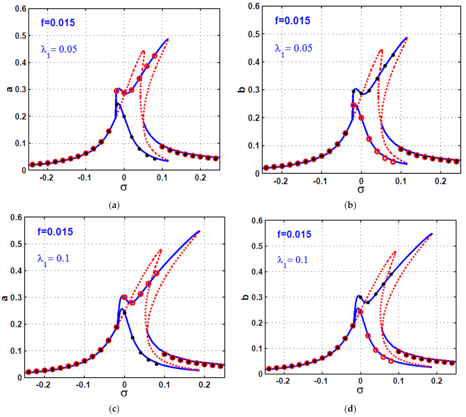
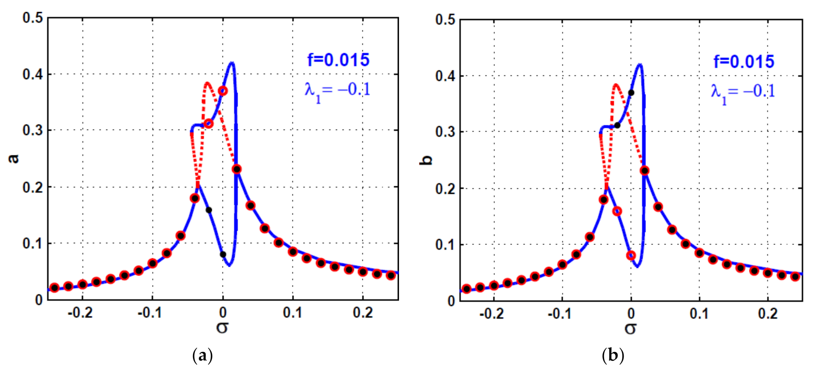
- Integrating the cubic position controller () into the linear controller makes the control algorithm more flexible to changing the system dynamical behaviours from the hardening spring characteristic to the softening spring characteristic (or vice versa) by designing the suitable values of without any constraints to avoid the resonance conditions.
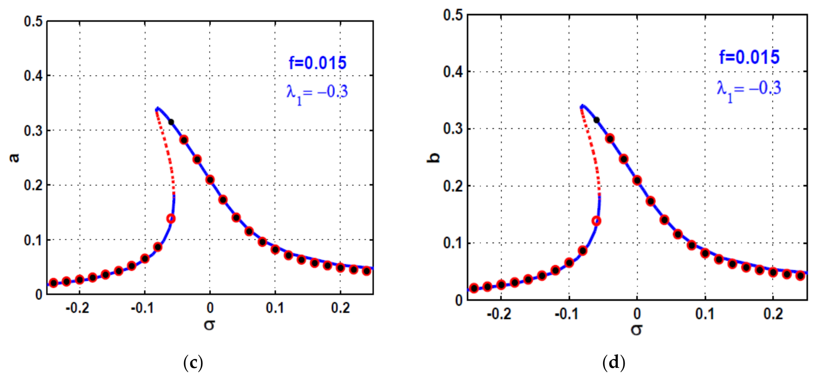
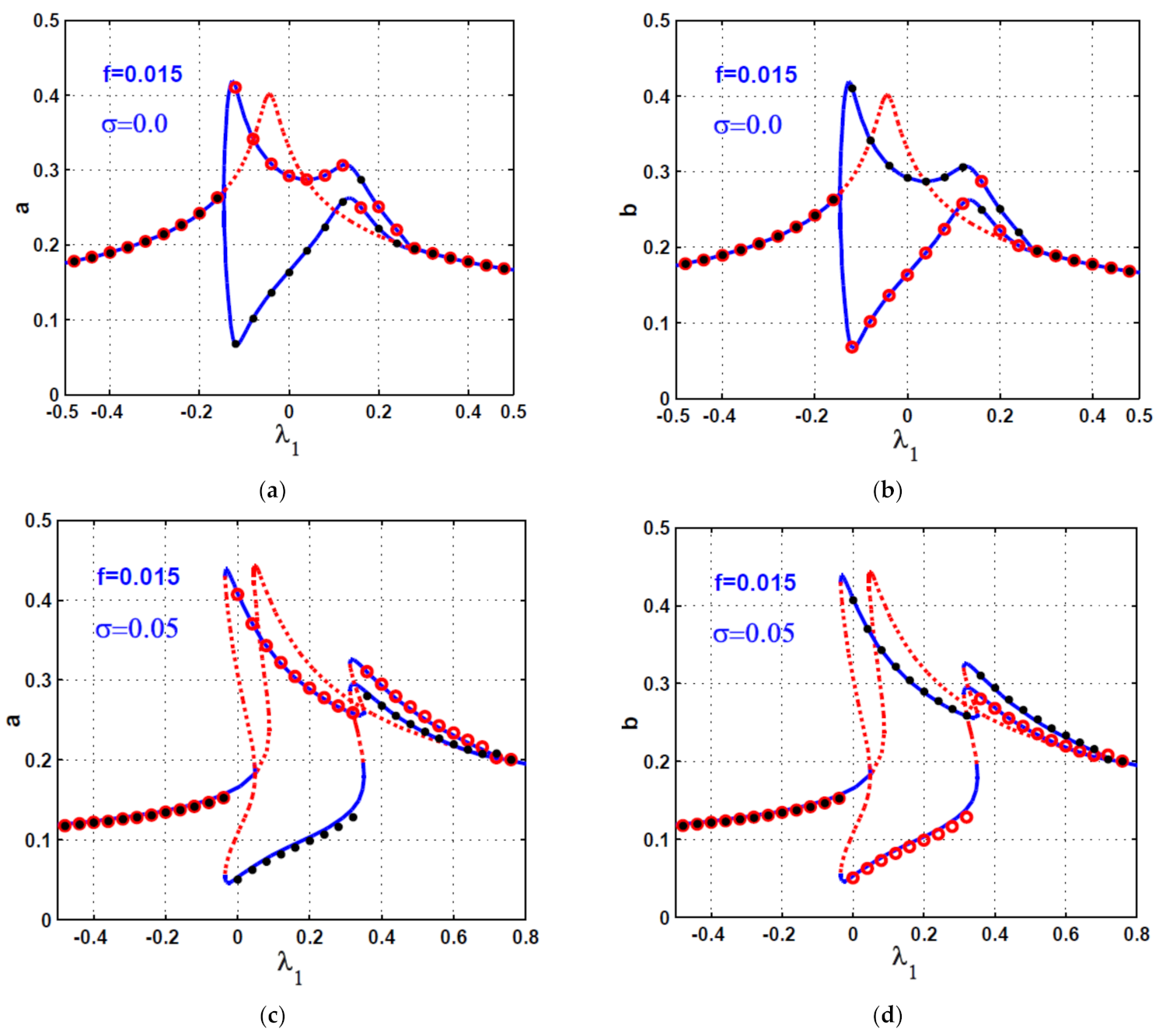
- Selecting the cubic position gain () with large negative values can simplify the system dynamical behaviours and mitigate system oscillations, even at resonance conditions.
- The good design of the cubic position gain (i.e., ) can stabilise the unstable motion and eliminate the nonlinear effects of the system at large disc eccentricities.
- Integrating the cubic velocity controller () to the linear controller added a nonlinear damping term to the controlled system that improved system stability or destabilised its motion, depending on the control gain sign.
- The optimal design of the cubic velocity gain (i.e., ) could stabilise the unstable motion and eliminate the nonlinear effects of the system at large disc eccentricities
Author Contributions
Funding
Institutional Review Board Statement
Informed Consent Statement
Data Availability Statement
Acknowledgments
Conflicts of Interest
Abbreviations
| Dimensionless displacement, velocity, and acceleration of the RAMBS in direction. | |
| Dimensionless displacement, velocity, and acceleration of the RAMBS in direction. | |
| Dimensionless linear damping coefficient of the RAMBS in and directions. | |
| Dimensionless linear natural frequency of the RAMBS in and directions. | |
| Dimensionless disc spinning-speed of the RAMBS. | |
| Dimensionless disc eccentricity of the RAMBS. | |
| Dimensionless control gain of the linear position controller. | |
| Dimensionless control gain of the linear velocity controller. | |
| Dimensionless control gain of the cubic position controller. | |
| Dimensionless control gain of the cubic velocity controller. | |
| Dimensionless nonlinearity coupling coefficients. | |
| The detuning parameter, where . | |
| Steady-state vibration amplitudes of the RAMBS in and directions, respectively. | |
| Steady-state phase angles of the RAMBS in and directions, respectively. |
Appendix A
Appendix B
References
- Ji, J.C.; Yu, L.; Leung, A.Y.T. Bifurcation behavior of a rotor supported by active magnetic bearings. J. Sound Vib. 2000, 235, 133–151. [Google Scholar] [CrossRef]
- Saeed, N.A.; Awwad, E.M.; El-Meligy, M.A.; Nasr, E.S.A. Radial Versus Cartesian Control Strategies to Stabilize the Nonlinear Whirling Motion of the Six-Pole Rotor-AMBs. IEEE Access 2020, 8, 138859–138883. [Google Scholar] [CrossRef]
- Saeed, N.A.; Mahrous, E.; Awrejcewicz, J. Nonlinear dynamics of the six-pole rotor-AMBs under two different control configurations. Nonlinear Dyn. 2020, 101, 2299–2323. [Google Scholar] [CrossRef]
- Ji, J.C.; Hansen, C.H. Non-linear oscillations of a rotor in active magnetic bearings. J. Sound Vib. 2001, 240, 599–612. [Google Scholar] [CrossRef]
- Saeed, N.A.; Eissa, M.; El-Ganini, W.A. Nonlinear oscillations of rotor active magnetic bearings system. Nonlinear Dyn. 2013, 74, 1–20. [Google Scholar] [CrossRef]
- Ji, J.C.; Leung, A.Y.T. Non-linear oscillations of a rotor-magnetic bearing system under superharmonic resonance conditions. Int. J. Nonlinear Mech. 2003, 38, 829–835. [Google Scholar] [CrossRef]
- Yang, X.D.; An, H.Z.; Qian, Y.J.; Zhang, W.; Yao, M.H. Elliptic Motions and Control of Rotors Suspending in Active Magnetic Bearings. J. Comput. Nonlinear Dyn. 2016, 11, 054503. [Google Scholar] [CrossRef]
- Saeed, N.A.; Mahrous, E.; Abouel Nasr, E.; Awrejcewicz, J. Nonlinear dynamics and motion bifurcations of the rotor active magnetic bearings system with a new control scheme and rub-impact force. Symmetry 2021, 13, 1502. [Google Scholar] [CrossRef]
- Zhang, W.; Zhan, X.P. Periodic and chaotic motions of a rotor-active magnetic bearing with quadratic and cubic terms and time-varying stiffness. Nonlinear Dyn. 2005, 41, 331–359. [Google Scholar] [CrossRef]
- Zhang, W.; Yao, M.H.; Zhan, X.P. Multi-pulse chaotic motions of a rotor-active magnetic bearing system with time-varying stiffness. Chaos Solitons Fractals 2006, 27, 175–186. [Google Scholar] [CrossRef]
- Zhang, W.; Zu, J.W.; Wang, F.X. Global bifurcations and chaos for a rotor-active magnetic bearing system with time-varying stiffness. Chaos Solitons Fractals 2008, 35, 586–608. [Google Scholar] [CrossRef]
- Zhang, W.; Zu, J.W. Transient and steady nonlinear responses for a rotor-active magnetic bearings system with time-varying stiffness. Chaos Solitons Fractals 2008, 38, 1152–1167. [Google Scholar] [CrossRef]
- Li, J.; Tian, Y.; Zhang, W.; Miao, S.F. Bifurcation of multiple limit cycles for a rotor-active magnetic bearings system with time-varying stiffness. Int. J. Bifurc. Chaos 2008, 18, 755–778. [Google Scholar] [CrossRef]
- Li, J.; Tian, Y.; Zhang, W. Investigation of relation between singular points and number of limit cycles for a rotor–AMBs system. Chaos Solitons Fractals 2009, 39, 1627–1640. [Google Scholar] [CrossRef]
- Saeed, N.A.; Kandil, A. Two different control strategies for 16-pole rotor active magnetic bearings system with constant stiffness coefficients. Appl. Math. Model. 2021, 92, 1–22. [Google Scholar] [CrossRef]
- Kandil, A.; Sayed, M.; Saeed, N.A. On the nonlinear dynamics of constant stiffness coefficients 16-pole rotor active magnetic bearings system. Eur. J. Mech. A/Solids 2020, 84, 104051. [Google Scholar] [CrossRef]
- Wu, R.; Zhang, W.; Yao, M.H. Nonlinear vibration of a rotor-active magnetic bearing system with 16-pole legs. In Proceedings of the International Design Engineering Technical Conferences and Computers and Information in Engineering Conference, Cleveland, OH, USA, 6–9 August 2017. [Google Scholar] [CrossRef]
- Wu, R.; Zhang, W.; Yao, M.H. Analysis of nonlinear dynamics of a rotor-active magnetic bearing system with 16-pole legs. In Proceedings of the International Design Engineering Technical Conferences and Computers and Information in Engineering Conference, Cleveland, OH, USA, 6–9 August 2017. [Google Scholar] [CrossRef]
- Wu, R.Q.; Zhang, W.; Yao, M.H. Nonlinear dynamics near resonances of a rotor-active magnetic bearings system with 16-pole legs and time varying stiffness. Mech. Syst. Signal Process. 2018, 100, 113–134. [Google Scholar] [CrossRef]
- Zhang, W.; Wu, R.Q.; Siriguleng, B. Nonlinear Vibrations of a Rotor-Active Magnetic Bearing System with 16-Pole Legs and Two Degrees of Freedom. Shock Vib. 2020, 2020, 5282904. [Google Scholar] [CrossRef]
- Ma, W.S.; Zhang, W.; Zhang, Y.F. Stability and multi-pulse jumping chaotic vibrations of a rotor-active magnetic bearing system with 16-pole legs under mechanical-electric-electromagnetic excitations. Eur. J. Mech. A/Solids 2021, 85, 104120. [Google Scholar] [CrossRef]
- Eissa, M.; Saeed, N.A.; El-Ganini, W.A. Saturation-based active controller for vibration suppression of a four-degree-of-freedom rotor-AMBs. Nonlinear Dyn. 2014, 76, 743–764. [Google Scholar] [CrossRef]
- Saeed, N.A.; Kandil, A. Lateral vibration control and stabilization of the quasiperiodic oscillations for rotor-active magnetic bearings system. Nonlinear Dyn. 2019, 98, 1191–1218. [Google Scholar] [CrossRef]
- Ishida, Y.; Inoue, T. Vibration suppression of nonlinear rotor systems using a dynamic damper. J. Vib. Control 2007, 13, 1127–1143. [Google Scholar] [CrossRef]
- Saeed, N.A. On the steady-state forward and backward whirling motion of asymmetric nonlinear rotor system. Eur. J. Mech. A/Solids 2019, 80, 103878. [Google Scholar] [CrossRef]
- Saeed, N.A. On vibration behavior and motion bifurcation of a nonlinear asymmetric rotating shaft. Arch. Appl. Mech. 2019, 89, 1899–1921. [Google Scholar] [CrossRef]
- Saeed, N.A.; Awwad, E.M.; El-Meligy, M.A.; Nasr, E.S.A. Sensitivity analysis and vibration control of asymmetric nonlinear rotating shaft system utilizing 4-pole AMBs as an actuator. Eur. J. Mech. A/Solids 2021, 86, 104145. [Google Scholar] [CrossRef]
- Saeed, N.A.; Awwad, E.M.; El-Meligy, M.A.; Nasr, E.S.A. Analysis of the rub-impact forces between a controlled nonlinear rotating shaft system and the electromagnet pole legs. Appl. Math. Model. 2021, 93, 792–810. [Google Scholar] [CrossRef]
- Oueini, S.S.; Nayfeh, A.H. Single-mode control of a cantilever beam under principal parametric excitation. J. Sound Vib. 1999, 224, 33–47. [Google Scholar] [CrossRef]
- Chen, L. Vibration suppression of a principal parametric resonance. J. Vib. Control 2009, 15, 439–463. [Google Scholar] [CrossRef]
- Pratiher, B. Vibration control of a transversely excited cantilever beam with tip mass. Arch. Appl. Mech. 2012, 82, 31–42. [Google Scholar] [CrossRef]
- Huang, D.; Xu, W. Sensitivity analysis of primary resonances and bifurcations of a controlled piecewise-smooth system with negative stiffness. Commun. Nonlinear Sci. Numer. Simulat. 2017, 52, 124–147. [Google Scholar] [CrossRef]
- Joyce, B.S.; Tarazaga, P.A. Mimicking the cochlear amplifier in a cantilever beam using nonlinear velocity feedback control. J. Smart Mater. Struct. 2014, 23, 1–5. [Google Scholar] [CrossRef]
- Warminski, J.; Bochenski, M.; Jarzyna, W.; Filipek, P.; Augustyniak, M. Active suppression of nonlinear composite beam vibrations by selected control algorithms. Commun. Nonlinear Sci. Numer. Simulat. 2011, 16, 2237–2248. [Google Scholar] [CrossRef]
- Jun, L.; Rongying, S.; Hongxing, H. Cubic velocity feedback control of high-amplitude vibration of a nonlinear plant to a primary resonance excitation. Shock Vib. 2007, 14, 1–14. [Google Scholar] [CrossRef]
- Ghaderi, N.; Keyanpour, M. Anti-collocated observer-based output feedback control of wave equation with cubic velocity nonlinear boundary and Dirichlet control. Int. J. Control 2020, 1–11. [Google Scholar] [CrossRef]
- Chen, L.; Cao, T.; He, F.; Sammut, K. Bifurcation control of a flexible beam under principal parametric excitation. In Proceedings of the American Control Conference, Chicago, IL, USA, 28–30 June 2000. [Google Scholar]
- Maccari, A. The response of a parametrically excited van der Pol oscillator to a time delay state feedback. Nonlinear Dyn. 2001, 26, 105–119. [Google Scholar] [CrossRef]
- Maccari, A. Vibration control for the primary resonance of the van der Pol oscillator by a time delay state feedback. Int. J. Nonlinear Mech. 2003, 38, 123–131. [Google Scholar] [CrossRef]
- Ishida, Y.; Yamamoto, T. Linear and Nonlinear Rotordynamics: A Modern Treatment with Applications, 2nd ed.; Wiley-VCH Verlag GmbH & Co. KGaA: New York, NY, USA, 2012. [Google Scholar] [CrossRef]
- Schweitzer, G.; Maslen, E.H. Magnetic Bearings: Theory, Design, and Application to Rotating Machinery; Springer: Berlin/Heidelberg, Germany, 2009. [Google Scholar] [CrossRef]
- Nayfeh, A.H.; Mook, D.T. Nonlinear Oscillations; Wiley: New York, NY, USA, 1995. [Google Scholar] [CrossRef]
- Nayfeh, A.H. Resolving Controversies in the Application of the Method of Multiple Scales and the Generalized Method of Averaging. Nonlinear Dyn. 2005, 40, 61–102. [Google Scholar] [CrossRef]
- Slotine, J.-J.E.; Li, W. Applied Nonlinear Control; Prentice Hall: Englewood Cliffs, NJ, USA, 1991. [Google Scholar]
- Yang, W.Y.; Cao, W.; Chung, T.; Morris, J. Applied Numerical Methods Using Matlab; John Wiley & Sons, Inc.: Hoboken, NJ, USA, 2005. [Google Scholar]
- Govaerts, W. Numerical Methods for Bifurcations of Dynamical Equilibria; SIAM: Philadelphia, PA, USA, 2000. [Google Scholar]


Publisher’s Note: MDPI stays neutral with regard to jurisdictional claims in published maps and institutional affiliations. |
© 2021 by the authors. Licensee MDPI, Basel, Switzerland. This article is an open access article distributed under the terms and conditions of the Creative Commons Attribution (CC BY) license (https://creativecommons.org/licenses/by/4.0/).
Share and Cite
El-Shourbagy, S.M.; Saeed, N.A.; Kamel, M.; Raslan, K.R.; Abouel Nasr, E.; Awrejcewicz, J. On the Performance of a Nonlinear Position-Velocity Controller to Stabilize Rotor-Active Magnetic-Bearings System. Symmetry 2021, 13, 2069. https://doi.org/10.3390/sym13112069
El-Shourbagy SM, Saeed NA, Kamel M, Raslan KR, Abouel Nasr E, Awrejcewicz J. On the Performance of a Nonlinear Position-Velocity Controller to Stabilize Rotor-Active Magnetic-Bearings System. Symmetry. 2021; 13(11):2069. https://doi.org/10.3390/sym13112069
Chicago/Turabian StyleEl-Shourbagy, Sabry M., Nasser A. Saeed, Magdi Kamel, Kamal R. Raslan, Emad Abouel Nasr, and Jan Awrejcewicz. 2021. "On the Performance of a Nonlinear Position-Velocity Controller to Stabilize Rotor-Active Magnetic-Bearings System" Symmetry 13, no. 11: 2069. https://doi.org/10.3390/sym13112069