Identification of Ship Dynamics Model Based on Sparse Gaussian Process Regression with Similarity

Abstract

The system identification of a ship dynamics model is crucial for the intelligent navigation and design of the ship’s controller. The fluid dynamic effect and the complicated geometry of the hull surface cause a nonlinear or asymmetrical behavior, and it is extremely difficult to establish a ship dynamics model. A nonparametric model based on sparse Gaussian process regression with similarity was proposed for the dynamic modeling of a ship. It solves the problem, wherein the kernel method is difficult to apply to big data, using similarity to sparse large sample datasets. In addition, the experimental data of the KVLCC2 ship are used to verify the validity of the proposed method. The results show that sparse Gaussian process regression with similarity can be applied to the learning of a large sample data, in order to obtain ship motion prediction with higher accuracy than the parameterized model. Moreover, in the case of sensor signal loss, the identified model continues to provide accurate ship speed and trajectory information in the future, and the maximum prediction error of the motion trajectory within 100 s is only 0.59 m.

1. Introduction

With the development of autonomous ship technology, the safety of the autonomous navigation of ships is particularly important. An accurate ship maneuvering model has a high practical value for providing accurate motion predictions or designing a control system. When the ship performs tasks that require high maneuverability, such as obstacle avoidance or navigation in narrow waters, the ship dynamics model is used to foresee the behavior or trajectory of the ship in the future, and judge whether the current control strategy is safe or the planned path meets the dynamic constraints. Then, the model takes the correct actions to avoid collisions.

The fluid dynamic effect and the complicated geometry of the hull surface cause a nonlinear or asymmetrical behavior, since establishing an accurate dynamic model is always a difficult problem in practical applications for ships. Currently, modeling of the ship maneuvering motion is mainly divided into parametric modeling based on a priori model and nonparametric modeling based on data. Both modeling methods have their own advantages and disadvantages.

In parametric modeling, many models have been proposed to approximate the ship dynamics. In particular, the quadratic Norrbin model [1] and cubic Abkowitz [2] model are widely used in surface ships. Methods such as the least square [3], extended Kalman filter (EKF) [4], and least squares support vector regression (LSSVR) [5,6] have been used to identify the hydrodynamic coefficients in the model. However, due to the correlation between the terms in the model, the parameter cancellation effect [7] makes some hydrodynamic coefficients very unstable. The optimal truncated singular value decomposition (T-SVD) [8] and optimal truncated least squares support vector regression (T-LSSVR) [9,10,11] are proposed to reduce the uncertainty of the estimated parameters. However, this problem is not yet completely solved. At the same time, since only a limited number of polynomials are used to approximate the model, the model’s accuracy is not yet ideal, especially in the surge velocity. The ‘true’ model structure of a ship is never known. The goal of building a model is to obtain accurate predictions, and to not necessarily obtain the correct model structure.

Nonparametric modeling requires almost no previous information of the model structure of the ship, which can also obtain accurate predictions. Machine learning techniques provide an effective way for the modeling of ships [12]. Methods such as support vector regression (SVR), locally weighted learning (LWL), and Gaussian process regression (GPR) have been used in modeling of the ship maneuvering motion. Generalized ellipsoidal basis function fuzzy neural networks [13] are used to model the movement of a large tanker. However, the structure of the neural network is more difficult to determine. The $\nu$-support vector regression ($\nu$-SVR) [14] is proposed to establish the maneuvering motion model and is validated by KVLCC2 ship experimental data. Moreover, it is based on structural risk minimization to overcome the shortcomings of neural networks that are easy to overfit. However, the parameters are difficult to adjust. A novel nonparametric identification modeling method based on locally weighted learning (LWL) [15] is used for ship dynamics modeling. It can provide higher modeling accuracy, but has the disadvantage of high computational complexity and long computational time. Kernel ridge regression (KRR) [16,17,18] trains the models with several random tests, while KRR requires the performance of a grid search for hyperparameter optimization. Gaussian process regression (GPR) can automatically optimize hyperparameters by maximizing the marginal likelihood function, and it can also overcome overfitting. It is widely used in the dynamic modeling of robotic arms [19] and racing cars [20]. Recently, it has also been introduced in the dynamic modeling of ships. Multi-output Gaussian processes are proposed to model a container ship [21]. A noisy input Gaussian process is proposed for ship dynamics modeling using simulated ship motion data with artificial noise [22].

In general, nonparametric modeling with the kernel function avoids the shortcomings of parametric modeling that require a knowledge of the model structure. The nonparametric model can obtain ship motion prediction with higher accuracy than the parametric model. Insufficient information can affect the generalization ability of the model. Both the parametric model and nonparametric model require a large sample of data to cover the state space, in order to ensure the generalization of the model. However, it is difficult to use nonparametric kernel methods for regression when the data sample is too large.

In this paper, a nonparametric model based on sparse Gaussian process regression with similarity was used for the dynamic modeling of a ship without assumptions in the mathematical model of the ship. It solves the problem, wherein the kernel method is difficult to apply to big data, using similarity to sparse large sample datasets. The experimental data of KVLCC2 ship are used to verify the validity of the proposed method. In the case of sensor signal loss, the identified model continues to provide accurate ship acceleration, speed, and trajectory information in the future. Moreover, the multi-step prediction model is used to provide accurate ship speed and position information in the future, and it provides important support for the autonomous navigation of ships.

The rest of the paper is organized as follows: Section 2 presents the ship parametric model and nonparametric model, and reviews the Gaussian Process regression algorithm. Section 3 describes the large sample sparse Gaussian process regression algorithm based on similarity. In Section 4, identification modeling and a systematic evaluation are conducted based on real data from KVLCC2 model tests. Finally, Section 5 presents the conclusions and suggestions for future work.

2. Models and Methods

2.1. Ship Parametric Dynamics Model and Nonparametric Dynamics Model

The goal of modeling ship maneuvering motion is to build mathematical models that, given the ship’s state, thrust, and rudder angle as inputs, yields the best fit between the measured response of the ship and the model predictions. The more accurate the mapping between the input and output, the smaller the gap between the real world and the model.

The ship dynamics parametric model is extremely complex. In addition, the model contains radiation-induced added mass, potential damping, and restoring forces. Many parametric mathematical models describe the ship dynamics and most of the hydrodynamic equations are approximated by polynomials [13].

$$\left(m-X_{\dot{u}}\right)\dot{u}=f_1\left(u,v,r,\delta \right)$$

(1a)

$$\left(m-Y_{\dot{v}}\right)\dot{v}+\left(m{x}_G-Y_{\dot{r}}\right)\dot{r}=f_2\left(u,v,r,\delta \right)$$

(1b)

$$\left(m{x}_G-N_{\dot{v}}\right)\dot{v}+\left(I_z-N_{\dot{r}}\right)\dot{r}=f_3\left(u,v,r,\delta \right)$$

(1c)

where $f_1$, $f_2$, and $f_3$ are the polynomials related to the state information, as shown in Equation (2a)–(2c).

$$\begin{gathered} f_1\left(u,v,r,\delta \right)=X_u\Delta u+X_{uu}\Delta u^2+X_{uuu}\Delta u^3+X_{vv}{v}^2+X_{rr}{r}^2+X_{rv}rv+X_{\delta \delta }{\delta }^2+X_{u\delta \delta }\Delta u{\delta }^2+X_{v\delta }v\delta \\ +X_{uv\delta }\Delta uv\delta \end{gathered}$$

(2a)

$$\begin{gathered} f_2\left(u,v,r,\delta \right)=Y_{v}v+Y_{r}r+Y_{vvv}{v}^3+Y_{vvr}{v}^{2}r+Y_{vu}v\Delta u+Y_{ru}r\Delta u+Y_{\delta }\delta +Y_{\delta \delta \delta }{\delta }^3+Y_{\delta u}\delta \Delta u+Y_{\delta uu}\delta \Delta u^2 \\ +Y_{\delta \delta v}v{\delta }^2+Y_{\delta vv}\delta v^2 \end{gathered}$$

(2b)

$$\begin{gathered} f_3\left(u,v,r,\delta \right)=N_{v}v+N_{r}r+N_{vvv}{v}^3+N_{vvr}{v}^{2}r+N_{vu}v\Delta u+N_{ru}r\Delta u+N_{\delta }\delta +N_{\delta \delta \delta }{\delta }^3+N_{\delta u}\delta \Delta u+N_{\delta uu}\delta \Delta u^2 \\ +N_{\delta \delta v}v{\delta }^2+N_{\delta vv}\delta v^2 \end{gathered}$$

(2c)

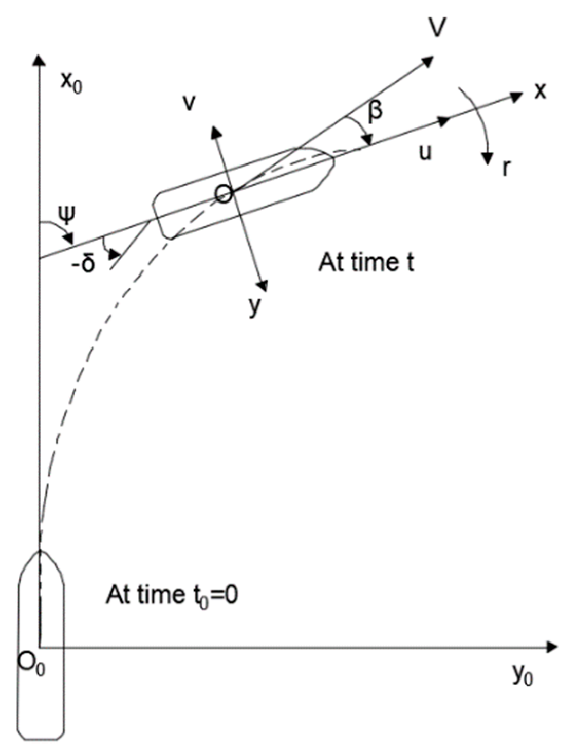
The relationship between the ship’s speed $V={\left[u,v,r\right]}^T$ and position$\eta ={\left[x_0,y_0,\psi \right]}^T$ is shown in Figure 1.

According to the expression form of the parametric model, this research model proposes a nonparametric model expression of the ship dynamics. Here, $f$ is no longer assumed to be a third-order Taylor expansion.

$$\dot{V}=f\left(V,\tau \right)$$

(3)

where $\tau$ is usually expressed by T, which is generated by the thruster and rudder $\delta$. The three DoF models can be represented as follows:

$${\dot{u}}_k=f_u\left(u_k,v_k,r_k,T_k,{\delta }_k\right)$$

(4)

$${\dot{v}}_k=f_v\left(u_k,v_k,r_k,T_k,{\delta }_k\right)$$

(5)

$${\dot{r}}_k=f_r\left(u_k,v_k,r_k,T_k,{\delta }_k\right)$$

(6)

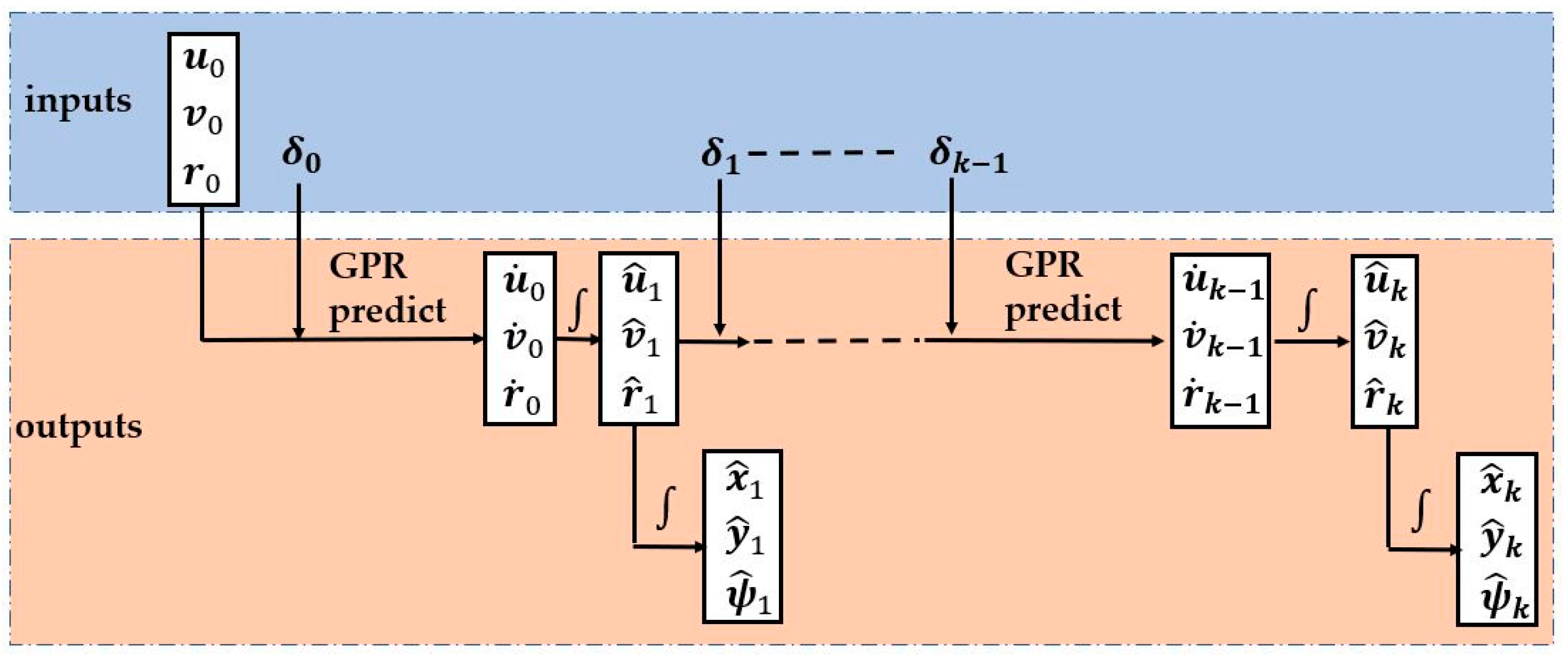
The purpose of traditional maneuvering motion prediction is for the verification of the maneuvering capabilities of the ship. Given this, the model completes the zigzag tests and turning circle tests in the simulation to obtain the maneuverability parameters (overshoot angles, advance, and tactical diameter, etc.) of the ship. However, the rudder angle in the simulation and the experiment is not always the same. Moreover, when planning a route or controlling a ship to avoid obstacles, the operator would like to know whether the predicted state response or trajectory of the ship is consistent with the actual situation after executing a series of control commands. Therefore, it is necessary to ensure that the control commands in the simulation and the test are the same at all times. The main inputs of the model are: Initial conditions $\left(u_0,v_0,r_0\right)$ and the commanded variables in the next k-steps (rudder angles $({\delta }_0,{\delta }_1,{\delta }_2,\dots {\delta }_{k-1}$). To simplify the model, the propellers speed $T$ can usually be regarded as a constant and not as an input variable. The outputs are the ship’s acceleration $\left(\dot{u},\dot{v},\dot{r}\right)$ in the next k-steps, and of course, the speed $\left(\widehat{u},\widehat{v},\widehat{r}\right)$ and position $\left[\widehat{x},\widehat{y},\widehat{\psi }\right]$ of the ship can be obtained through Euler integration. The inputs and the outputs of the model are shown in Figure 2.

2.2. Gaussian Process Regression

Here, $\left\{\left(x_i,y_i\right)|i=1,\cdots ,n\right\}$ are the inputs and outputs of the regression. The relationship between them can be expressed by

$$y_i=f\left(x_i\right)+\epsilon ,\epsilon ~N\left(0,{\mathsf{\sigma }}_n^2\right)$$

(7)

In the Gaussian process regression [23], the joint distribution of $y$ and $f(x^{*})$ is

$$\left[\begin{array}{c}y\\ f(x^{*})\end{array}\right]~N\left(0,\left[\begin{array}{cc}K\left(\mathrm{X},\mathrm{X}\right)+{\mathsf{\sigma }}_n{}^{2}I& K\left(x^{*},\mathrm{X}\right)\\ K\left(\mathrm{X},x^{*}\right)& K\left(x^{*},x^{*}\right)\end{array}\right]\right)$$

(8)

The prediction of $f(x^{*})$ is

$$f(x^{*})=k\left(x^{*},X\right){\left(\mathrm{K}\left(\mathrm{X},\mathrm{X}\right)+{\mathsf{\sigma }}_n{}^2{I}_n\right)}^{-1}y$$

(9)

$$Var\left[f(x^{*})\right]=k\left(x^{*},x^{*}\right)-k\left(x^{*},X\right){\left(\mathrm{K}\left(\mathrm{X},\mathrm{X}\right)+{\mathsf{\sigma }}_n{}^2{I}_n\right)}^{-1}k\left(X,x^{*}\right)$$

(10)

The proposed model adopts the commonly used squared exponential covariance function:

$$k\left(x_i,x_j\right)=f{\left(x_i\right)}^{T}f\left(x_j\right)={\mathsf{\sigma }}_f{}^2\exp (-\frac{1}{2}{(x_i-x_j)}^T\mathsf{\Lambda }\left(x_i-x_j\right)$$

(11)

where ${\mathsf{\sigma }}_f$ and $\mathsf{\Lambda }$ are the kernel’s hyperparameters. The hyperparameters on Gaussian process regression are computed using the conjugate gradient (CG) or Broyden-Fletcher-Goldfarb-Shanno (BFGS) algorithms on the marginal likelihood function.

$$-\log p\left(y|X,\theta \right)=\frac{1}{2}{y}^T{\left(\mathrm{K}\left(\mathrm{X},\mathrm{X}\right)+{\mathsf{\sigma }}_n{}^2{I}_n\right)}^{-1}y+\frac{1}{2}log\left|{\left(\mathrm{K}\left(\mathrm{X},\mathrm{X}\right)+{\mathsf{\sigma }}_n{}^2{I}_n\right)}^{-1}\right|+\frac{n}{2}log2\pi$$

(12)

Several other machine learning methods are used in ship dynamics modeling, such as Kernel Ridge regression (KRR) and least squares support vector regression (LSSVR). Compared with Gaussian process regression, they employ the same loss functions, while KRR and LSSVR require the performance of a grid search for hyperparameter optimization. The parameter selection in Gaussian process regression may be faster, as it does not suffer an exponential scaling.

3. Large Sample Sparse Gaussian Process Regression Algorithm Based on Similarity

Nonparametric modeling based on kernel methods, such as the Gaussian process is mainly suitable for interpolation prediction. When there are sample points near point $x^{*}$ that are required to be predicted, the prediction at $x^{*}$ will be more accurate. In order to learn a ‘good’ model, the training dataset requires the state space to be covered as much as possible.

Ship motion data are usually in the hundreds of thousands. Accurate modeling requires as many samples as possible to provide rich data incentives. However, when all of the sample points are used for regression prediction, it will cause the inverse matrix to be uncalculated. The easiest way to reduce the calculation of the inverse matrix is to select only a small part of the large sample data for modeling. The randomly selected data from a large sample will make the sample spatial distribution uneven. In addition, there may be no sample points in a local area that are close to point $x^{*}$ that require to be predicted, resulting in inaccurate predictions.

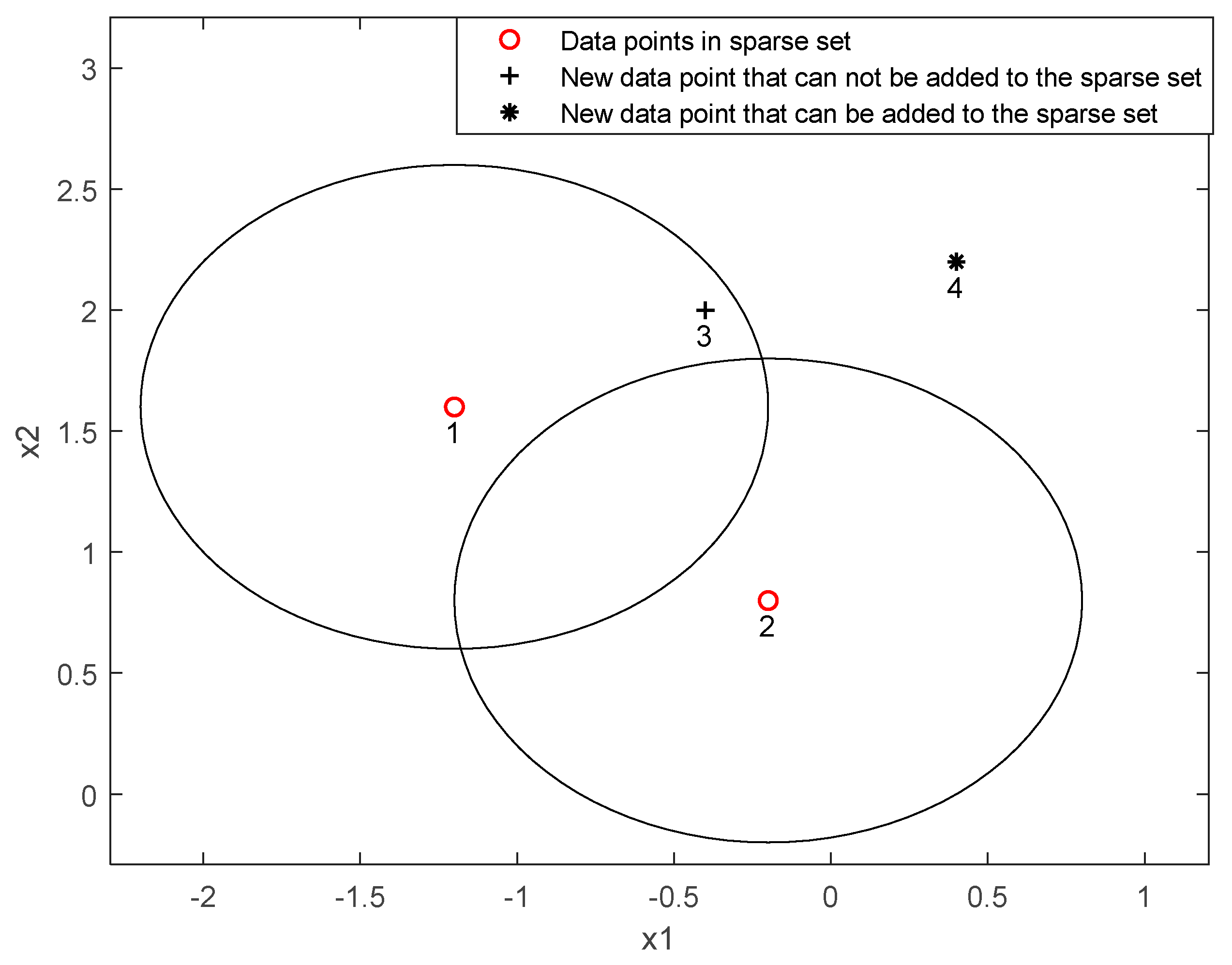
A sparse algorithm based on similarity is proposed to the sparse large sample data. Points with less similarity are equivalent to containing new incentives and are added to the sparse set. Points with greater similarity are regarded as information redundancy and are not added to the sparse set. A sparse set with a small uniform distribution in the shape space is obtained, which replaces the overall sample for regression prediction.

Taking a two-dimensional input system as an example, the similarity between $x_i$ and $x_j$ can be defined as

$$d\left(x_i,x_j\right)=\exp \left(-\frac{{(x_{i1}-x_{j1})}^2}{l_1^2}-\frac{{(x_{i2}-x_{j2})}^2}{l_2^2}\right)$$

(13)

The closer $x_i$ and $x_j$ are, the greater the similarity, and the similarity is 1 when they are completely similar. Moreover, $l_1$ and $l_2$ represent the weight coefficient of each dimension. Here, the larger the setting, the larger the interval between the data points selected for this dimension. Furthermore, it can usually be set to the amplitude of each dimension to balance the data points of each dimension.

Figure 3 shows the principle of updating sparse data based on similarity. The new data point 3 has a high similarity to the existing points in the sparse set. It is regarded as data redundancy and is not added to the sparse set. Point 4 is farther from the sparse set and is regarded as new information that is added to the sparse set.

$$y=x_1\sin \left(x_2\right)+x_2\sin \left(x_1\right)$$

(14)

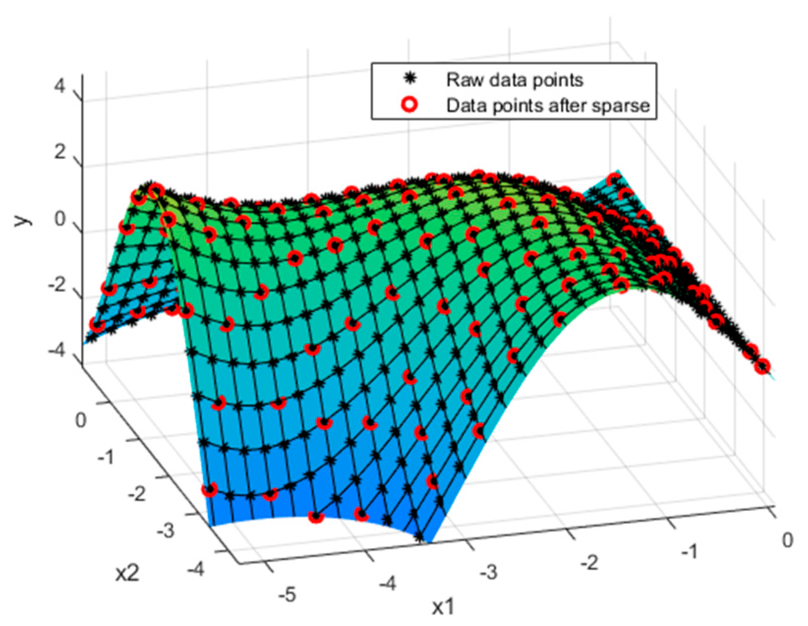
Taking two-dimensional surface reconstruction as an example, the data points are generated by the function in Equation (12). Both dimensions are sampled at 0.2 intervals for a total of 3721 sample points. The flowchart of learning based on the sparse Gaussian process is detailed in

Table 1. The flowchart of learning based on the sparse Gaussian process.

Algorithm	Sparse Gaussian Process
1	Set the similarity threshold $d_{gen}$ and the weight of each dimension $l$
2	Add the first data to the sparse set $S$. $M=1,S=\left\{x_1\right\}$
3	Determine whether the new data are similar to the sparse dataset $for i=2:N$
4	Calculate the similarity $d\left(x_i,S_j\right),j=1:M$
5	If $\max \left(d\left(x_i,S_j\right)\right)<d_{gen}$
6	Add new data $x_i$to the sparse set $S$. $S=S{\displaystyle \cup }\left\{x_i\right\},M=M+1$;end;end
7	Use sparse set $S$ rather than all of the datasets for Gaussian process regression

.

Figure 4 shows the distribution of data after sparseness, and the sparse data points are evenly distributed throughout the space.

Table 2. The influence of the number of sparse data on model prediction.

Number of Sparse Set Data	Prediction Error	Training Time	Prediction Time
3721	2.13 × 10−5	54.01 s	0.0057 s
1122	9.33 × 10−5	26.63 s	0.0032 s
723	1.08 × 10−4	7.14 s	0.0022 s
350	1.96 × 10−4	0.68 s	0.0016 s
142	5.12 × 10−3	0.29 s	0.0013 s

shows the influence of sparse data amount on model prediction accuracy and speed. It can be found that only 350 data points can be selected to achieve a similar prediction accuracy to 3721 samples. In addition, the training time is shortened from 54 to 0.6 s and the accuracy is satisfied. At the same time, it greatly saves training time.

4. Modeling of Ship Maneuvering Motion with Experimental Data

4.1. Experimental Ship Model and Dataset

A free-running test is a commonly used method for ship dynamics identification. This method only requires the measurement of the status information, such as the ship’s position and speed, and does not require the measurement of the force. In addition, it can be applied to full-scale ships to avoid scale effects.

KVLCC2 is a large oil tanker, which has been used as the benchmark ship type for the validation of maneuvering simulation methods in the world. The experimental data used in this study come from the KVLCC2 model free-running test conducted at the Hamburg water tank (HSVA) in Germany. The main parameters of the KVLCC2 model are detailed in

Table 3. Parameters and dimensions of the KVLCC2 model.

Parameters	Values
$L_{pp}$ (m)	7.0
$B$ (m)	1.2688
Displacement (${\mathrm{m}}^3$)	3.2724
Beam coefficient	0.8098
Nominal speed (m/s)	1.179
Rudder speed ($\dot{\delta }$)	15.8 deg/s

.

A series of standard zigzag maneuvers were tested. All of the data were collected with a sampling rate of 20 Hz. The experimental data used in this research are shown in

Table 4. Test data of the KVLCC2 model.

Maneuver	Max Rudder Angle (°)	Heading Change (°)	Data Points
15/5°	15	5	3660
20/5°	20	5	3500
25/5°	25	5	3660
30/5°	30	5	3960
35/5°	35	5	4160

.

4.2. Modeling by Different Training Data

The dataset under different rudder angle ranges may contain different dynamic characteristics. Only a dataset that can provide enough dynamic information allows the identification of a reliable model. Models trained on different training sets will obtain different accuracies for the same motion prediction. To analyze the impact of different training sets on the model accuracy, different training sets are set to train the model and the least square method is used to identify the model in Equation (2).

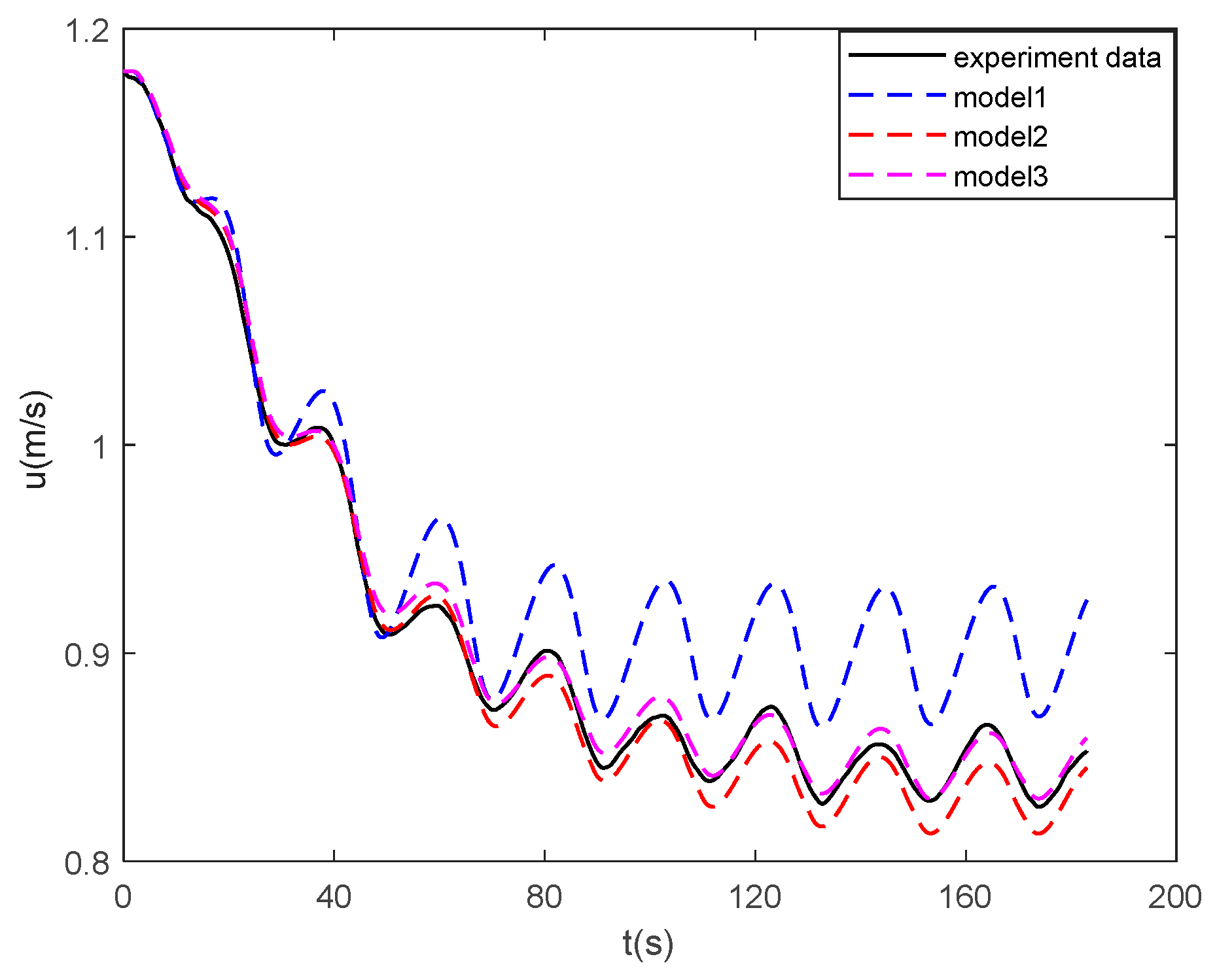
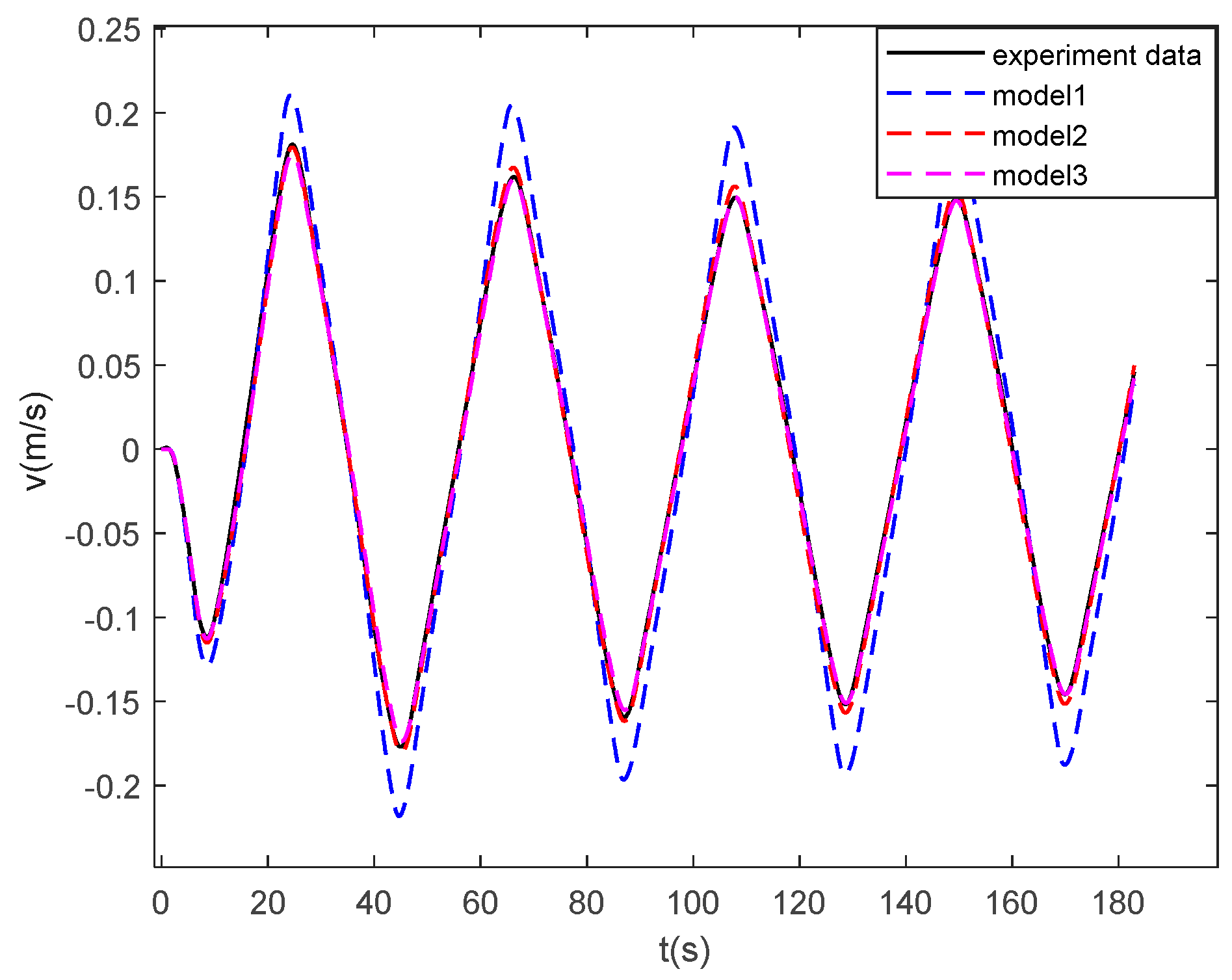
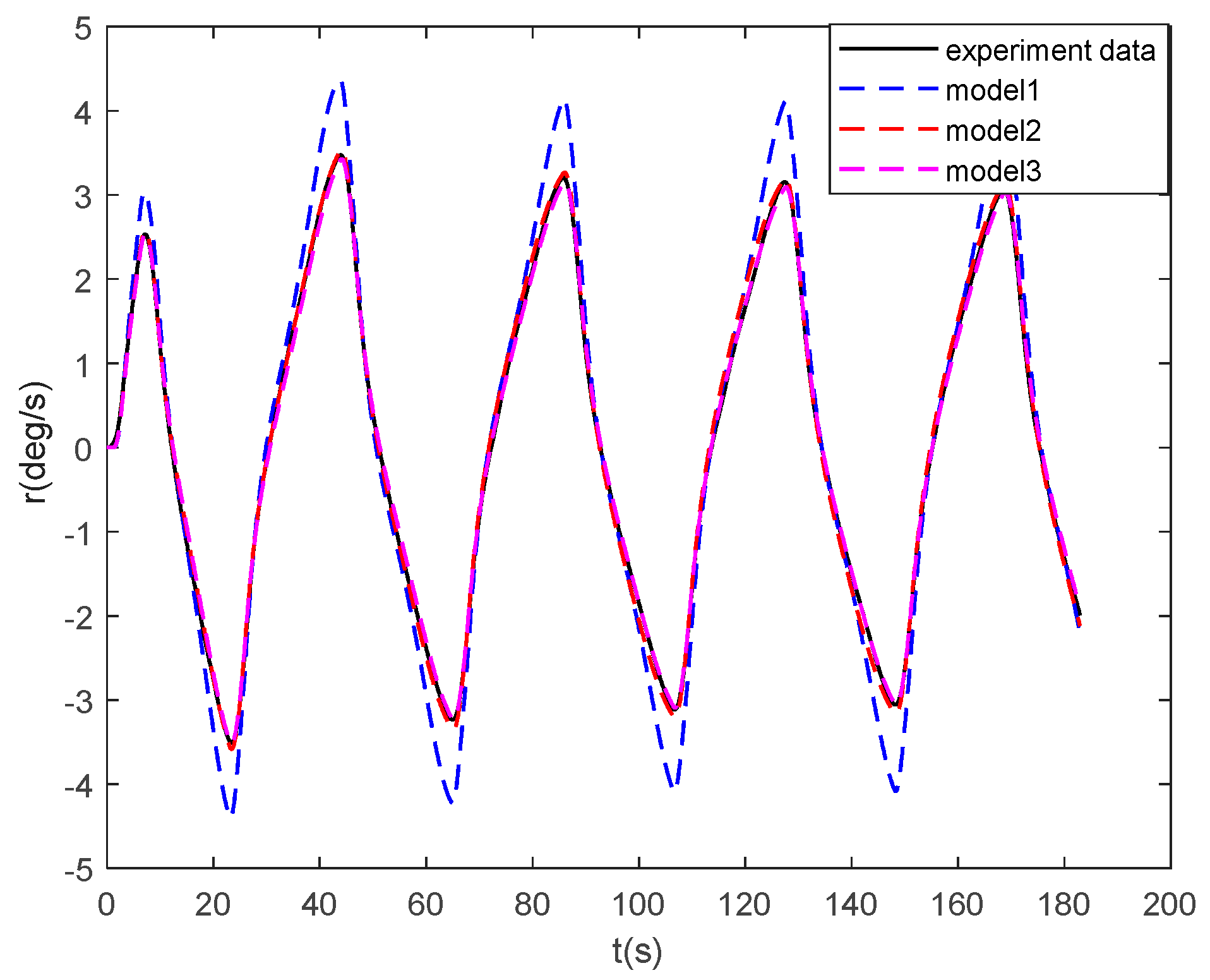
The root mean square deviation (RMSE) of speed in

Table 5. The RMSE of speed of different training sets.

Model	Training Set	Validation Set	$\mathbf{u}({10}^{-2}\mathbf{m}/\mathbf{s})$	$\mathbf{v}({10}^{-2}\mathbf{m}/\mathbf{s})$	$\mathbf{r}({10}^{-2}\mathbf{deg}/\mathbf{s})$
1	15/5°	25/5°	4.06	2.43	47.54
2	35/5°	25/5°	0.97	0.46	10.65
3	15/5°, 20/5°, 30/5°, 35/5°	25/5°	0.58	0.39	7.65

is applied to evaluate the preference of different models. The prediction results of different training sets are shown in Figure 5, Figure 6 and Figure 7. The results show that the prediction effect of the training set of a single rudder angle is significantly worse than the multiple rudder angles. When using model 3 as the training set, the rudder angle completely covers the state space. The prediction result almost coincides with the experimental data. However, there are still some errors in the surge speed between the prediction and the experimental data, which show that a few errors still remain in the approximation of the polynomial model of the surge.

4.3. Modeling by Sparse Gaussian Process Regression with Similarity

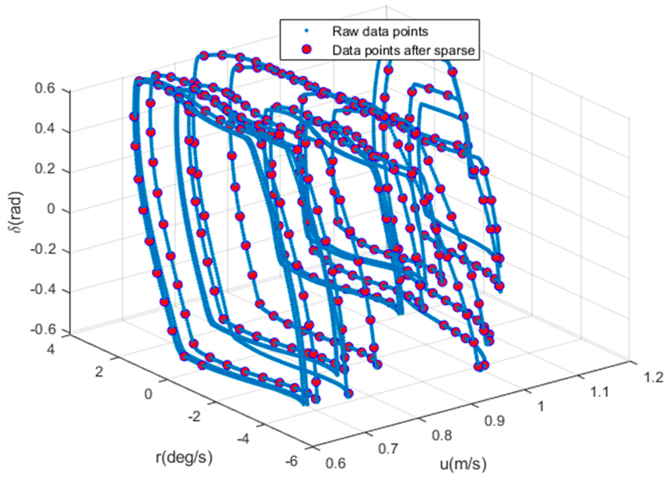
There is a certain error in using the finite term polynomial approximation model, especially when the surge model is not ideal. Therefore, the Gaussian process regression uses the infinite-dimensional kernel function, which can obtain a higher-precision model. Similar to the parametric model, in order to learn a ‘good’ model, the training data must cover a large range of the model state space. Briefly, 15/5°, 20/5°, 30/5°, and 35/5° zigzag tests are used to train the model. The data almost cover the input space of the steering angle. The training set data have a total of 15,280 data points. If Gaussian process regression is used directly, the inverse matrix is almost impossible to calculate. According to the sparse Gaussian process algorithm based on similarity in Table 1, the training set is sparsed. The 312 data points of the sparse dataset are evenly distributed in the state space, as shown in Figure 8.

The 15/5°, 20/5°, 30/5°, and 35/5° zigzag tests are used in the training set. The 25/5° zigzag test is treated as the validation set, and it is the same dataset that compares the prediction accuracy of the sparse Gaussian process model and the parameter model.

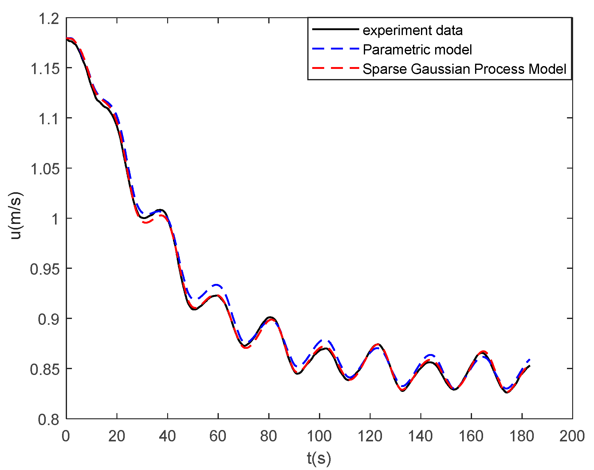
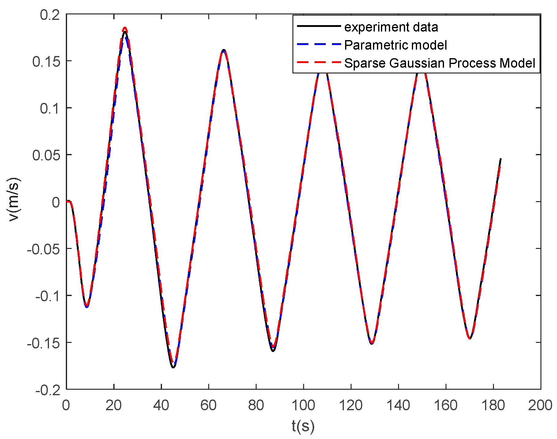
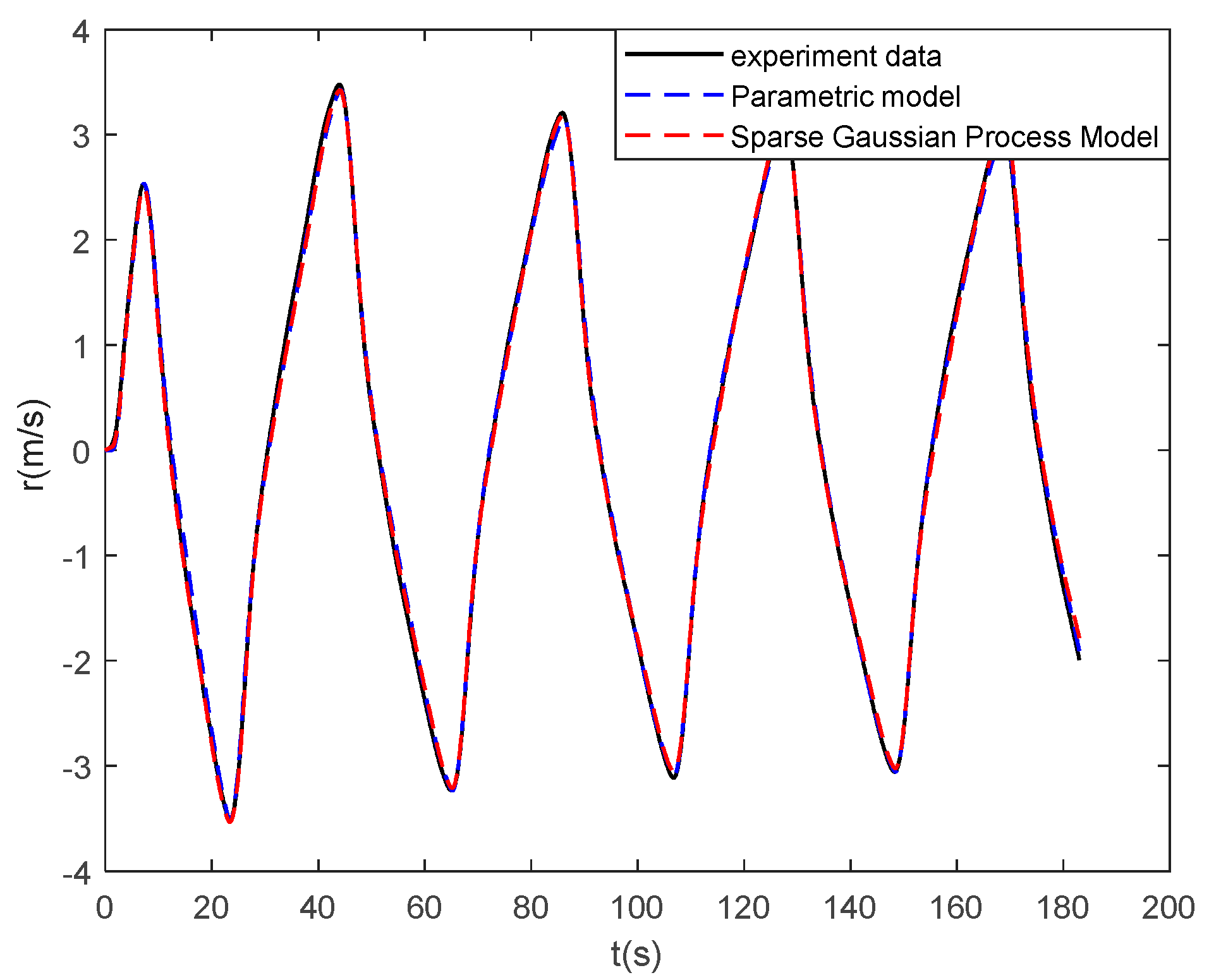
The prediction results of different training sets are shown in Figure 9, Figure 10 and Figure 11. The RMSE of speed in

Table 6. The RMSE of speed of different methods.

Methods	$\mathbf{u}({10}^{-2}\mathbf{m}/\mathbf{s})$	$\mathbf{v}({10}^{-2}\mathbf{m}/\mathbf{s})$	$\mathbf{r}({10}^{-2}\mathbf{deg}/\mathbf{s})$
Sparse Gaussian Process Model	0.25	0.35	7.25
Parametric Model	0.58	0.39	7.65

is applied to evaluate the preference of different methods. From the results, compared with the parametric model, the prediction of the sparse Gaussian process method has significantly improved the accuracy of surge velocity. Moreover, the prediction result almost coincides with the experimental data. There is a small difference between the two methods in predicting the sway velocity and yaw rate, and it is almost consistent with the experiment. It proves that the parametric model of surge velocity can still be further improved.

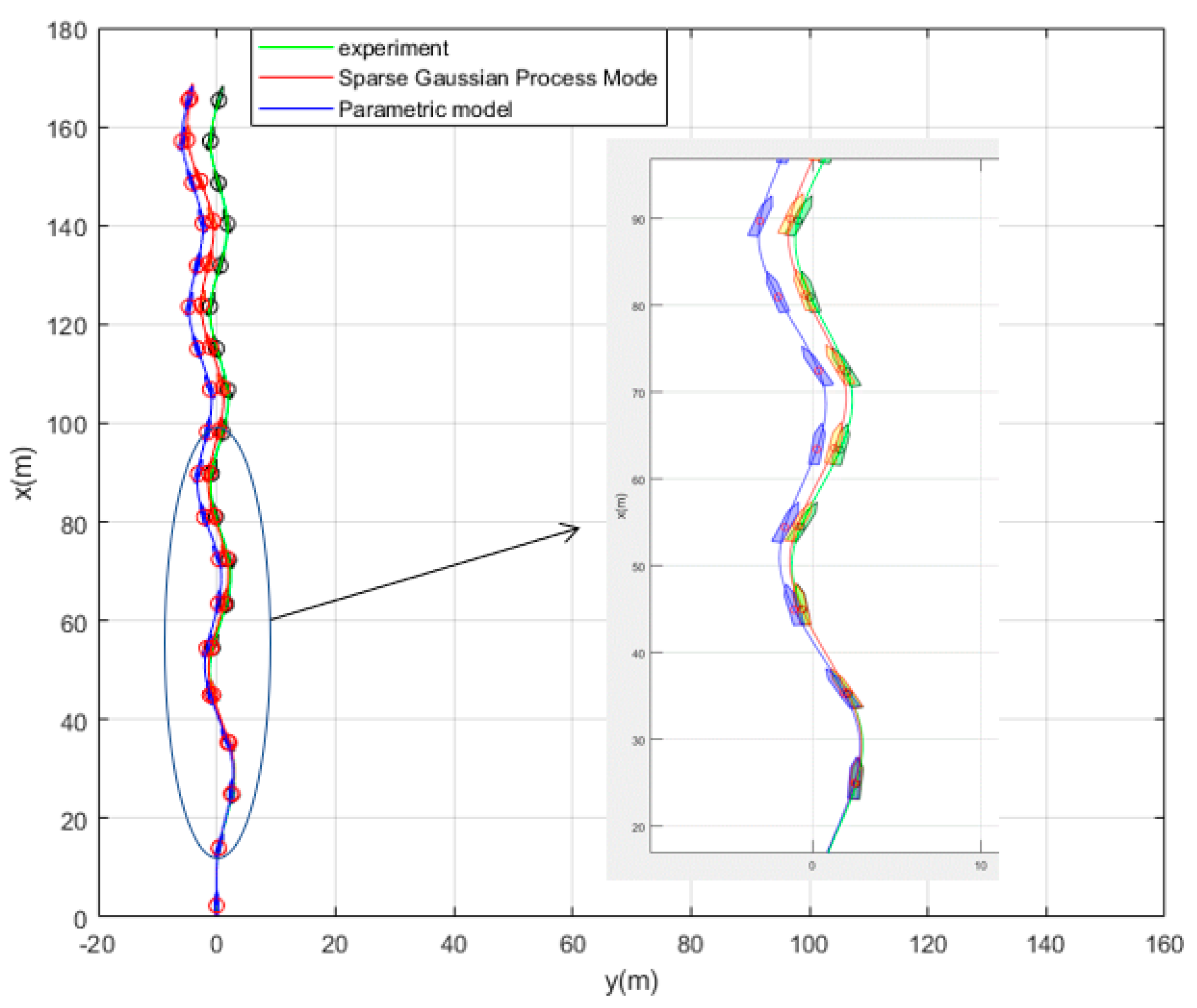
The trajectory $\left[\widehat{x},\widehat{y},\widehat{\psi }\right]$ of the ship can be obtained through Euler integration. Figure 12 shows the result of trajectory prediction. It can be found that in the short-term prediction, the sparse Gaussian process prediction trajectory nearly coincides with the experimental trajectory, and the accuracy is higher than the parameter model prediction. The maximum prediction error of 100 s is only 0.59 m, and the maximum error of the parameter model prediction reaches 3.21 m. With the increase in the number of prediction steps, the error will have a certain cumulative error. Nevertheless, the ship’s trajectory predicted by the sparse Gaussian process continues to follow the experimental trajectory with a small error.

5. Conclusions and Future Work

In this work, a data-driven nonparametric model based on sparse Gaussian process regression with similarity was used for the dynamic modeling of a ship. The experimental data of KVLCC2 are used to verify the validity of the proposed method. The case study shows that the sparse Gaussian process regression with similarity can be applied to the learning of large sample data and to obtain ship motion prediction with higher accuracy than the parameterized model. In the case of sensor signal loss, the model can continue to provide accurate ship state information in the future, and the maximum error of 100 s trajectory prediction is 0.59 m. High-precision prediction can help controllers make safe decisions on path planning and obstacle avoidance.

The advantages of the proposed model based on sparse Gaussian process regression with similarity for ship dynamics modeling can be summarized as follows: First, unlike parameter identification, the model based on Gaussian process regression is not required to know the previous model structure of the ship dynamics. It obtains a more accurate motion prediction than the parametric model. Second, the similarity-based sparse method solves the defect, wherein the kernel method is difficult to apply to large sample data learning. It only uses very little data to replace the large sample information. Therefore, the model can be more generalized. Finally, the Gaussian process is the same as LSSVR and KRR in mean prediction. The hyperparameters learned by the Gaussian process can be used in the two aforementioned methods. In addition, the proposed sparse algorithm can be applied to the two aforementioned algorithms.

However, the proposed method still requires further research. Since the information contained in the dataset determines the essential performance of the model, it is difficult to further improve the model performance without increasing the training data. For parametric and nonparametric identification, the training data should cover the ship motion state space as much as possible. Moreover, further research is required to understand how the least experimentation can be used to cover the state space.

References

- Abkowitz, M.A. Measurements of hydrodynamic characteristics from ship maneuvering trials by system identification. Trans. SNAME 1980, 88, 283–318. [Google Scholar]
- Norrbin, N.H. Ship Manoeuvring with Application to Shipborne Predictors and Real-Time Simulators. J. Mech. Eng. Sci. 1972, 14, 91–107. [Google Scholar] [CrossRef]
- Holzhuter, T. Robust identification scheme in an adaptive track-controller for ships. IFAC Proc. Vol. 1990, 23, 461–466. [Google Scholar] [CrossRef]
- Yoon, H.K.; Rhee, K.P. Identification of hydrodynamic coefficients in ship maneuvering equations of motion by Estimation-Before-Modeling technique. Ocean Eng. 2003, 30, 2379–2404. [Google Scholar] [CrossRef]
- Luo, W.L.; Moreira, L.; Soares, C.G. Manoeuvring simulation of catamaran by using implicit models based on support vector machines. Ocean Eng. 2014, 82, 150–159. [Google Scholar] [CrossRef]
- Zhu, M.; Hahn, A.; Wen, Y.Q. Identification-based simplified model of large container ships using support vector machines and artificial bee colony algorithm. Appl. Ocean Res. 2017, 68, 249–261. [Google Scholar] [CrossRef]
- Luo, W.L.; Li, X. Measures to diminish the parameter drift in the modeling of ship manoeuvring using system identification. Appl. Ocean Res. 2017, 67, 9–20. [Google Scholar] [CrossRef]
- Xu, H.; Hassani, V.; Soares, C.G. Parameters Estimation of Nonlinear Manoeuvring Model for Marine Surface Ship Based on PMM Tests. In ASME 2018 37th International Conference on Ocean, Offshore and Arctic Engineering; American Society of Mechanical Engineers: Madrid, Spain, 2018. [Google Scholar] [CrossRef]
- Xu, H.; Soares, C.G. Experimental investigation of shallow water effect on vessel steering model using system identification method. Ocean Eng. 2017, 199, 106940. [Google Scholar] [CrossRef]
- Xu, H.; Hassani, V.; Soares, C.G. Uncertainty analysis of the hydrodynamic coefficients estimation of a nonlinear manoeuvring model based on planar motion mechanism tests. Ocean Eng. 2019, 173, 450–459. [Google Scholar] [CrossRef]
- Xu, H.; Hinostroza, M.; Hassani, V.; Soares, C.G. Real-time parameter estimation of nonlinear vessel steering model using support vector machine. J. Offshore Mech. Arct. Eng. 2019, 141, 061606. [Google Scholar] [CrossRef] [Green Version]
- Duan, L.; Iseki, T. A new estimation concept for hydrodynamic derivatives of ship manoeuvrability using machine learning toolkits. In Developments in Maritime Technology and Engineering; CRC Press: London, UK, 2021; pp. 169–176. [Google Scholar] [CrossRef]
- Wang, N.; Er, M.J.; Han, M. Large Tanker Motion Model Identification Using Generalized Ellipsoidal Basis Function-Based Fuzzy Neural Networks. IEEE Trans. Cybern. 2015, 45, 2732–2743. [Google Scholar] [CrossRef] [PubMed]
- Wang, Z.; Xu, H.; Xia, L.; Zou, Z.; Soares, C.G. Kernel-based support vector regression for nonparametric modeling of ship maneuvering motion. Ocean Eng. 2014, 216, 107994. [Google Scholar] [CrossRef]
- Bai, W.; Ren, J.; Li, T. Modified genetic optimization-based locally weighted learning identification modeling of ship maneuvering with full scale trial. Future Gener. Comput. Syst. 2019, 93, 1036–1045. [Google Scholar] [CrossRef]
- Moreno-Salinas, D.; Moreno, R.; Pereira, A.; Aranda, J.; de la Cruz, J.M. Modeling of a surface marine vehicle with kernel ridge regression confidence machine. Appl. Soft Comput. 2019, 76, 237–250. [Google Scholar] [CrossRef]
- Moreno, R.; Moreno-Salinas, D.; Aranda, J. Black-box marine vehicle identification with regression techniques for random manoeuvres. Electronics 2019, 8, 492. [Google Scholar] [CrossRef] [Green Version]
- Moreno, R.; Besada-Portas, E.; Aranda, J. Symbolic regression for marine vehicles identification. IFAC-Pap. 2015, 48, 210–216. [Google Scholar] [CrossRef]
- Carron, A.; Arcari, E.; Wermelinger, M.; Hewing, L.; Zeilinger, M.N. Data-driven model predictive control for trajectory tracking with a robotic arm. IEEE Robot. Autom. Lett. 2019, 4, 3758–3765. [Google Scholar] [CrossRef] [Green Version]
- Kabzan, J.; Hewing, L.; Liniger, A. Learning-based model predictive control for autonomous racing. IEEE Robot. Autom. Lett. 2019, 4, 3363–3370. [Google Scholar] [CrossRef] [Green Version]
- Ramire, W.A.; Leong, Z.Q.; Hung, N.; Jayasinghe, S.G. Non-parametric dynamic system identification of ships using multi-output Gaussian Processes. Ocean. Eng. 2018, 166, 26–36. [Google Scholar] [CrossRef] [Green Version]
- Xue, Y.; Liu, Y.; Ji, C.; Xue, G.; Huang, S. System identification of ship dynamic model based on Gaussian process regression with input noise. Ocean Eng. 2020, 216, 107862. [Google Scholar] [CrossRef]
- Rasmussen, C.E.; Williams, K.I. Gaussian Processes for Machine Learning; Williams, C.K., Rasmussen, C.E., Eds.; MIT Press: Cambridge, MA, USA, 2006; pp. 8–31. [Google Scholar]
Figure 1.
Earth and ship-fixed coordinate systems.
Figure 2.
The inputs and outputs of the model.
Figure 3.
Data sparseness based on similarity.
Figure 4.
Data distribution after sparseness.
Figure 5.
Prediction error of surge speed at 25/5° under different training sets.
Figure 6.
Prediction error of sway speed at 25/5° under different training sets.
Figure 7.
Prediction error of yaw rate at 25/5° under different training sets.
Figure 8.
Figure 9.
Prediction error of surge speed at 25/5° under different methods.
Figure 10.
Prediction error of sway speed at 25/5° under different methods.
Figure 11.
Prediction error of yaw rate at 25/5° under different methods.
Figure 12.
Prediction of trajectory at 25/5° zigzag maneuver.