
Hyperspectral Image Classification Based on Cross-Scene Adaptive Learning


Heilongjiang Province Key Laboratory of Laser Spectroscopy Technology and Application, Harbin University of Science and Technology, Harbin 150080, China
*
Author to whom correspondence should be addressed.
Symmetry 2021, 13(10), 1878; https://doi.org/10.3390/sym13101878
Submission received: 27 August 2021
/
Revised: 18 September 2021
/
Accepted: 29 September 2021
/
Published: 5 October 2021
Abstract
:Aiming at few-shot classification in the field of hyperspectral remote sensing images, this paper proposes a classification method based on cross-scene adaptive learning. First, based on the unsupervised domain adaptive technology, cross-scene knowledge transfer learning is carried out to reduce the differences between source scene and target scene. At the same time, depthwise over-parameterized convolution is used in the deep embedding model to improve the convergence speed and feature extraction ability. Second, two symmetrical subnetworks are designed in the model to further reduce the differences between source scene and target scene. Then, Manhattan distance is learned in the Manhattan metric space in order to reduce the computational cost of the model. Finally, the weighted K-nearest neighbor is introduced for classification, in which the weighted Manhattan metric distance is assigned to the clustered samples to improve the processing ability to the imbalanced hyperspectral image data. The effectiveness of the proposed algorithm is verified on the Pavia and Indiana hyperspectral dataset. The overall classification accuracy is 90.90% and 65.01%. Compared with six other kinds of hyperspectral image classification methods, the proposed cross-scene method has better classification accuracy.
1. Introduction
Hyperspectral sensor (i.e., spectral imager) images the object to be detected at the same time in tens to hundreds of continuous and subdivided spectral bands of the electromagnetic spectrum. Hyperspectral sensing images (HSI) are three-dimensional images combining space with spectrum information [1]. With rich third-dimensional information, it can more accurately subdivide and identify ground objects from the spectral space and has been widely used in military target reconnaissance [2], forestry monitoring [3], vegetation research [4], agriculture [5], chemistry [6,7,8], environmental science [9,10] and other fields. However, the labeled samples of hyperspectral images are limited, and manual collection of labeled samples for hyperspectral data is time-consuming and expensive. Therefore, how to use limited samples for classification processing without expanding the data source becomes important [11].
In the early stage of hyperspectral image classification, researchers only used spectral information for classification, including K-nearest neighbor (KNN) [12], random forest (RF) [13], support vector machine (SVM) [14,15], etc. Although these traditional methods effectively solved the problem of spectral information redundancy, they still have limitations. These methods do not deeply study the inherent spatial structure information of hyperspectral data, and it is difficult for the classification model to effectively handle the phenomena of “different body with same spectrum” or “same body with different spectrum” [16,17]. To solve this problem, researchers incorporated spatial information into hyperspectral classification and developed methods such as extended morphological profile (EMP). Liu et al., proposed a visual saliency-based extended morphological profile (VS-EMP) model, which is combined with SVM to improve the classification accuracy [18]. However, the feature extraction of this method depends on manual settings, and the implementation process is slightly complex.
In recent years, due to the powerful performance of deep learning in automatic feature extraction and learning different hierarchical structures, it has been widely used in the field of image classification [19]. In particular, convolutional neural networks (CNN), with its powerful feature expression ability, has been successfully applied to HSI classification [20,21,22,23,24,25]. In order to achieve better classification results, the above methods often need a large number of training samples. However, it is difficult to obtain labeled samples, which will make it more difficult for researchers to train network models. In order to alleviate this problem, Pan et al., proposed the multi-grained network (MugNet) network, which can be regarded as a simplified deep learning model. The multi-grained scanning strategy makes full use of optical spectrum and spatial information to improve the feature acquisition ability of the model and uses the semi supervised method to generate convolution kernel for reducing the model’s dependence on samples [26]. Sun et al., combined the attention mechanism with CNN to suppress the influence of interfering pixels, capture the most significant features, and improve CNN’s ability to distinguish ground objects [27]. He et al., proposed a heterogeneous transfer learning method to fully train the VGG-16Net network model on ImageNet and adjust the network parameters to transfer to hyperspectral data sets to complete effective classification [28]. Although the above methods reduce the dependence of models on samples to a certain extent, these models still need a certain amount of training samples to achieve better classification results.
In order to further reduce the dependence of the model on samples, some researchers have proposed a classification model suitable for small sample HSI data classification in recent years. Yang et al., proposed a new network called relationship network, which can learn and compare the categories of samples based on the similarity measure between sample pairs [29]. Rao et al., proposed the space-spectral relationship network to measure the deep similarity between samples and to increase the discrimination ability of the model to a small number of features by exploring the similarity measure between different samples [30]. Zhang et al., proposed a global prototype network, which projects the original data space into the embedded feature space, learns the vectors represented by the global prototype, and completes the classification by using KNN classifier through the similarity between vectors [31]. Although these classification models are better for small samples classification, it is easy to encounter the problem that the data to be classified does not have labeled samples in practical applications. The above classification models cannot obtain the similarity between samples and classify them effectively.
Because labeling samples is time-consuming and laborious, many HSI scenarios contain a small number of or unlabeled samples. However, with the increase of the number of HSI, a similar HSI scenario can still be found [32]. Some researchers have proposed a cross-scene classification method, which uses a similar source hyperspectral scene with large labeled samples to classify a target hyperspectral scene with no labeled samples or only a few labeled samples [33]. Kemker et al., input a large number of source scene data into the stacked convolution automatic encoder to learn similar features, and the obtained encoder can be used to classify the target scene through the fine-tuning process [34]. Due to the differences between different hyperspectral scenes, the source scene cannot be directly used to train the classifier. However, this method does not fully consider the differences between different scenes, which is also a major problem faced by cross-scene HSI classification. Therefore, Du et al., proposed the idea of domain adaptation to reduce the differences between different scenes and transfer knowledge for target scene classification by learning the features of a public subspace [35]. Deng et al., proposed a cross-scene classification model based on depth metric learning, using unsupervised domain adaptation technology to reduce the differences between different scenes and effectively use the source scene to classify the target scene [36]. However, this method still has shortcomings, such as ignoring the insufficient feature acquisition ability of traditional 2D convolutional neural network [37] and the imbalance of data categories in hyperspectral data [38].
This paper proposes a cross-scene adaptive learning classification model, which can reduce the dependence of the model on samples and enhance the processing ability of the model to handle the imbalance of data categories. Compared with the traditional methods (RBF-SVM, EMP-SVM) and deep learning methods (DCNN, ED-DMM-UDA, MDDUK, MDUWK), the classification accuracy has been significantly improved. The rest of this paper is organized as follows. Section 2 briefly introduces the relevant algorithms and improvements in this paper. Section 3 describes the experimental results and analysis of this paper. Section 4 summarizes the conclusions and future work.
2. The Proposed Methods
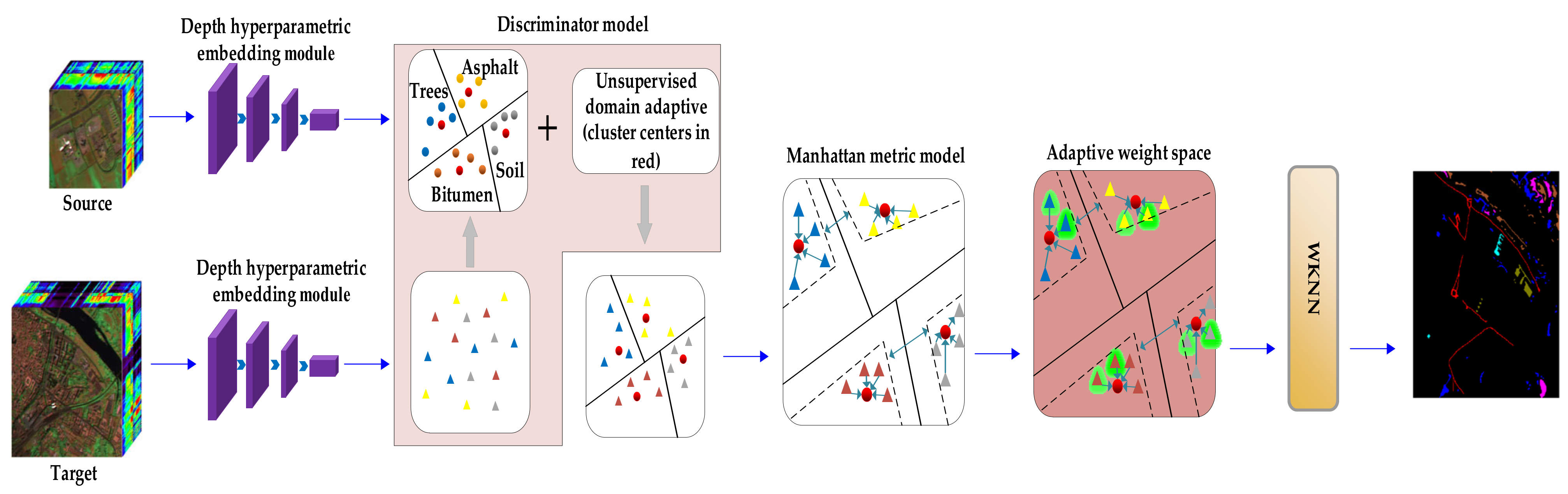
The cross-scene classification model proposed in this paper is shown in Figure 1. It can be seen from the figure that the model is composed of four core parts: deep hyperparameter embedding model, discriminator model, Manhattan metric model and WKNN classifier. The scene with training samples is called source scene, and the scene without training samples is called target scene.
First, the samples of different scenes are input into the depth hyperparametric embedding model, and the multi-dimensional feature extraction of the depth hyperparametric convolution layer is used to generate clusters with the same category, The same size embedding spaces are generated through the network with symmetrical structure to reduce the difference between the source scene and the target scene. Then, the clustered samples are projected into the discriminator, and the unsupervised domain adaptive technology is used to transfer cross-scene knowledge, such that the target scene forms a distribution similar to the source scene. Then, the processed target scene samples are mapped into Manhattan metric space to learn metric distance of any two samples, and the samples close to the cluster center are given greater weight. Finally, the final classification result is obtained by weighted K-nearest neighbor classifier.
2.1. The Deep Hyperparametric Embedding Model
The deep hyperparametric embedding model is composed of deep convolution neural network (DCNN) and depthwise over-parameterized convolution (DO-Conv). After the introduction of DO-Conv, the ability of automatic feature extraction across scene models is retained, and the problem of slow convergence caused by the depth of embedded model layers is made up. The model can also be regarded as a feature extractor in the cross-scene model. In order to extract the features of small samples more effectively, a smaller convolution kernel will be set in the feature extractor. The small convolution kernel will reduce the receptive field of the neural network, but increasing the size of the convolution kernel will also increase the parameter of the network model, which is not conducive to small sample training. Therefore, Li et al., proposed a depthwise over-parameterized convolution. Using the depthwise over-parameterized convolution instead of the conventional convolution layer without changing the size of the convolution kernel can accelerate the convergence speed of the model, add learnable parameters to the model, and will not increase the computational complexity [39]. There are two composition methods in DO-Conv, namely feature composition and convolution kernel composition. This paper trains the network by using the composition of convolution kernel in the depth hyperparametric embedding model to improve computation efficiency.
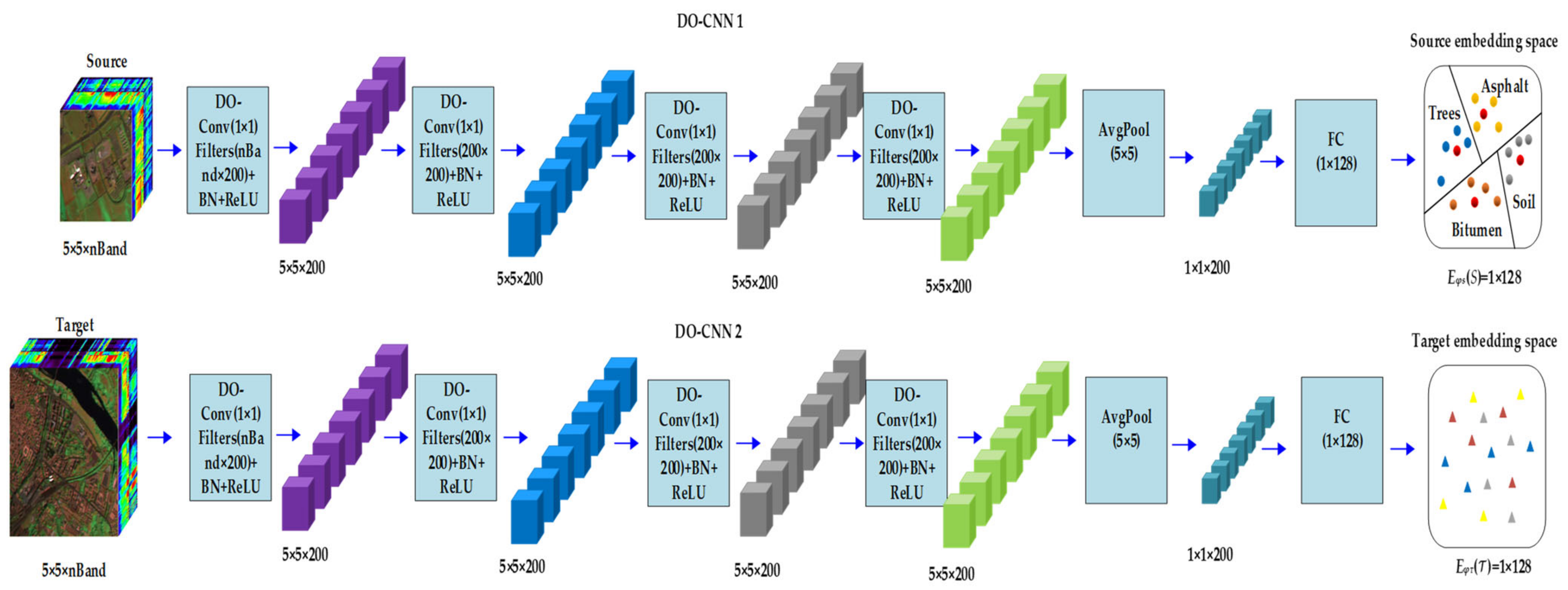
First, in order to learn the embedded features, the training samples are defined as , where is the total number of training samples. Each source training sample and target training sample have the corresponding tag values and . The embedded source features are defined as and the target features are defined as . In this space, the data reconstruction of the original samples is realized to form clusters with similar samples, as to better project the samples to the Manhattan metric space. The depth hyperparametric embedding model is shown in Figure 2, dots of different colors represent different categories, and red circles represent cluster centers. The output of each layer of deep hyperparametric embedding model is given in Figure 2. The deep superparametric embedding model in this paper is composed of two subnetworks, DO-CNN1 and DO-CNN2, with symmetrical structure. Symmetrical structure means that the layers and parameter settings of each sub network are the same, which is to obtain samples with the same output size and reduce the differences of the source scene and the target scene, such that the source scene can better guide the classification of target scenes.
DO-CNN1 consists of a deep hyperparametric convolution layer, batch normalization (BN), ReLU activation function, average pooling(AvgPool) and full connection layer (FC). In order to train a small number of samples more effectively, the size of depth hyperparametric convolution kernel is set to , where padding is 0, stripe is 1, the size of average pooling kernel is , and the size of full connection layer is . Assuming that the input sample is , the low-level features are extracted through the first layer of hyperparametric convolution, and the feature map with size is output. Then higher-level features are extracted from the samples by the second, third and fourth layers to generate a feature map with a size of. The sample size is compressed in the input to the average pooling layer, and the output feature map with is size of . Finally, the full connection layer is connected to the network output size of . The output of each layer of DO-CNN2 is the same as that of DO-CNN1. Finally, an embedding space with the size of is formed, which is the source embedding space and the target embedding space .
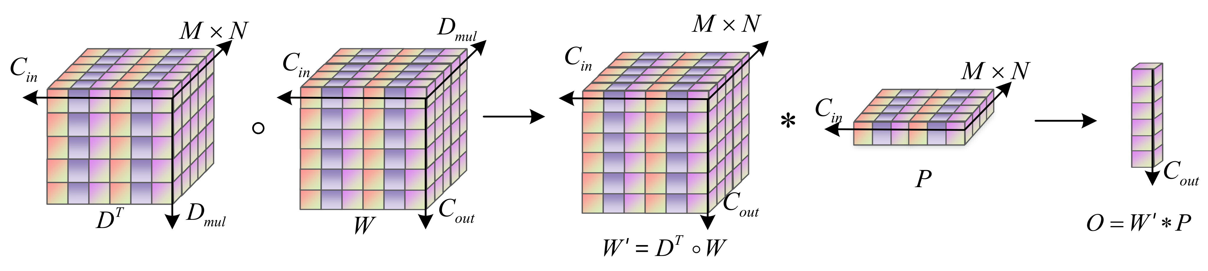
Depthwise over-parameterized convolution is composed of a conventional convolution and a depthwise convolution . In conventional convolution, the convolution layer processes the input data in a sliding way, and each element of the output feature is obtained from the horizontal section of a convolution kernel and the dot product of image blocks . In the deep convolution layer, the deep convolution kernel is convoluted with each input channel in the training stage. After the training stage, the multi-layer composite linear operation used for over parameterization is folded into a compact single-layer representation. Then, only a single layer is used in reasoning, which reduces the calculation to complete equivalence with the conventional layer.
In Figure 3, and is the spatial dimension of , is the number of input feature map, is the number of depth convolutions, is the number of output feature map, is the transpose of , and the convolution kernel of DO-Conv is . First combine the depth convolution kernel with the convolution kernel of ordinary convolution to generate , then convolutes to output features .
2.2. The Discriminator Model
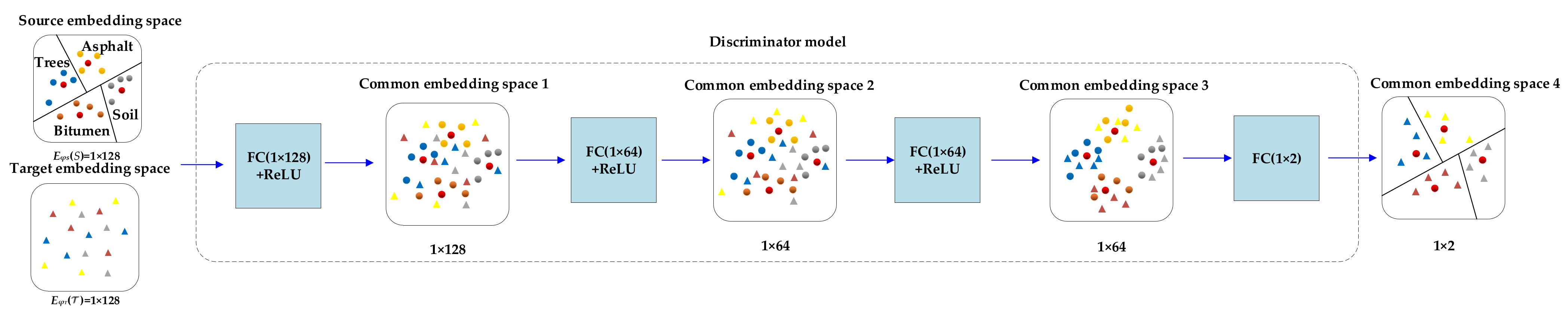
The purpose of the discriminator model is to reduce the difference between the source scene and the target scene through unsupervised domain adaptive technology, such that the target scene forms a distribution similar to the source scene, as to better project it into the metric space. The network structure is shown in Figure 4. It is composed of full connection layer (FC), batch normalization (BN) and ReLU activation function. The input is two isolated embedding spaces, which are the source embedding space and the target embedding space size of . The two isolated embedding spaces are mapped into common embedding space1 through the first full connection layer () to learn the characteristics of the source scene in this space. After optimizing common embedding space 1 by the second full connection layer of (), the size of common embedding “space2” is . Then, the third full connection layer () further optimizes the common embedding space2 to make the target scene form a distribution similar to the source scene, such as common embedding space 3. However, it contains the samples of the source scene. Therefore, the samples of the source scene are removed through the last full connection layer (), and the samples of the target scene are left alone to generate common embedding space4.
The difference between different scenes is reduced by the confusion discriminator. The definition of the domain confusion loss function is shown in Equation (2), where, and are the parameters of the target embedding model and the discriminator module , respectively, and the feature embedding distribution between the source and target is adjusted by .
The discriminator trains to confuse the source scene and the target scene, and trains to distinguish the embedding features and of the two scenes in the projected space, and constantly update the embedding space of the target scene.
The clustering center is calculated by the average value of the measurement of class embedding features. The minimization Equation (4) will promote the scene embedding to form a distribution similar to the scene , which helps the discriminator to confuse the differences between the data of the source scene and the target scene, such that the target scene can better learn the source scene.
2.3. Manhattan Metric Model
Manhattan metric model converts the metric distance of samples into a beneficial structure of metric space by learning the metric distance of samples because the distance metric has the characteristics of small intraclass spacing and large interclass spacing [40]. The reconstructed space still has the characteristics of high dimension of hyperspectral data. In order to retain the characteristic information of different dimensions, this paper uses Manhattan metric to obtain the attributes of samples, which has less computation than the commonly used European measurement and makes up for the shortcoming that the European measurement method does not consider the variability of values in all dimensions [41]. Manhattan distance metric will reduce the calculation cost of cross-scene model, which is defined as follows:
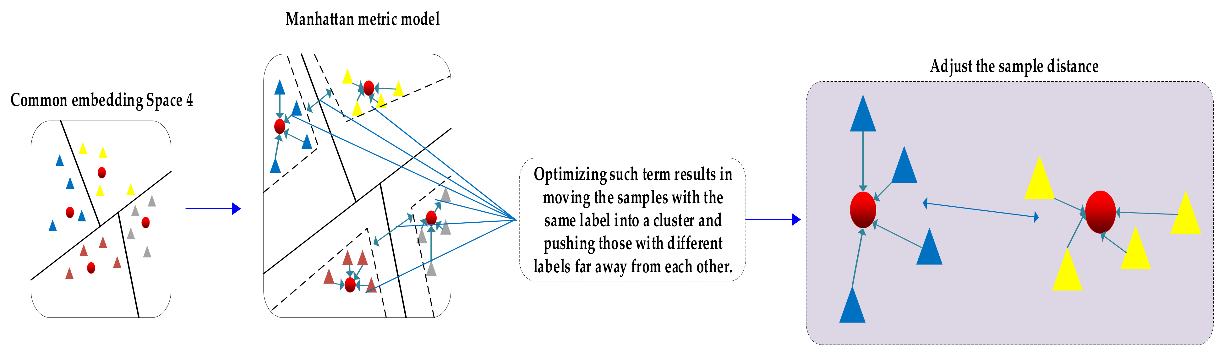
After any and two samples are embedded in the Manhattan metric model of the reconstructed space, their metric values can be calculated through the Manhattan metric model, as shown in Figure 5. are the embedding features formed by different samples after embedding the model, and the corresponding metric values are generated after passing the metric model.
The triplet loss where samples and have the same label, and have a different label. It is clear that Equation (6) encourages the embedding of to be closer to than to by at least margin 1. Optimizing such term results in moving the samples with the same label into a cluster and push those with different labels far away from each other. Therefore, an expected embedding is shown in Figure 5, which allows us to efficiently implement classification by using the KNN classifier based on the metric distance that we defined in (5) (Manhattan distance would be in this case).
2.4. The Weighted K-Nearest Neighbor
In order to improve the processing ability of the cross-scene model for unbalanced data of data categories, different weights are given to the samples after passing through the Manhattan metric model. The weighted classifier is called the weighted K-nearest neighbor (WKNN). First, this paper defines the adaptive weight of each class of sample in hyperspectral data set as shown in Equation (7), where is the weight of each class sample, is the category of sample and is the number of class samples.
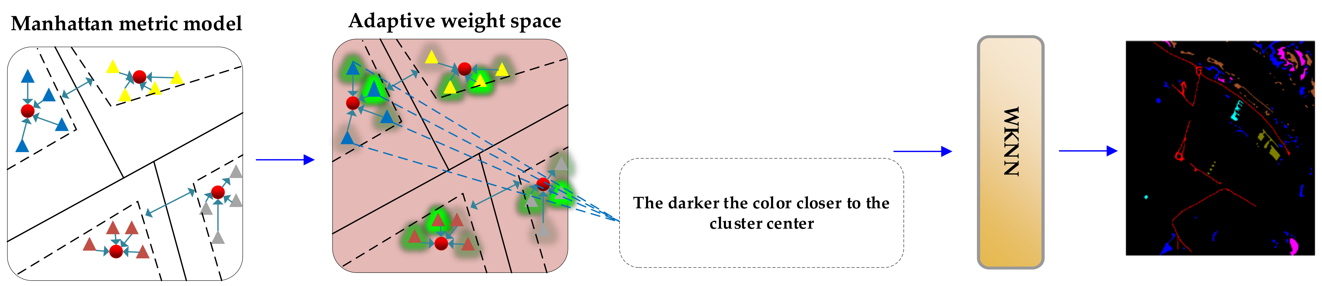
It can be seen from Table 1 that the weight of each type of sample in the Indiana and Pavia dataset. In the Indiana dataset, wheat is 3.65, 6.86 and 6.55 times higher than concrete/asphalt, orchard, soybeans and cleantill EW. It can be found that these two data have the characteristics of data category imbalance. However, the traditional KNN classifier is difficult to effectively process the category imbalance data [42]. This is bound to make it difficult to classify cross-scene hyperspectral data and the loss of feature information of some sample points will reduce the discrimination ability of the model to ground objects. Therefore, this paper gives adaptive weight to different sample points in Manhattan metric space, in which the weight is automatically transformed according to sample distance. As shown in Figure 6, the darker the color of the sample points, the greater the weight. This kind of sample points provide the most significant feature information for the model, which will improve the robustness of the model.
In order to enable KNN to process the category imbalance data more effectively, this paper increases the weight of the samples close to the embedding center , which are considered to contribute more to the classification, and give less weight to the samples with less contribution. In WKNN, the Manhattan distance calculated by the metric model is sorted and the corresponding weight is assigned, and then the nearest neighbor sample points are found to calculate the occurrence probability of the category, the category to which the sample with the highest probability of occurrence belongs is the category of the ground object finally determined by KNN classifier. The weight is as shown in Equation (8), and the weighted distance is as shown in Equation (9) where represents the distance information of the class sample.
3. Experimental Results and Analysis
3.1. Experimental Datasets Description
In order to verify the effectiveness of the proposed model for hyperspectral data classification, two public hyperspectral data sets, Indiana and Pavia, are used to test the classification algorithm. Indiana scene data was acquired by AVIRIS sensor in Northwest Tippecanoe country [43]. Two separate datasets were selected as the source scene and the target scene, both of which have the same size 400 × 300 and 220 bands. The two scenarios share seven land cover classes for classification. Pavia scene data is obtained from the DAIS sensor over the area of Pavia City, Italy. The size of Pavia University was 243 × 243 × 72 as the source scene image for training, the size of the central area of Pavia is 400 × 400 × 72 as the target scene image [44]. The two scenarios share six land cover classes for classification. The details of the two data sets are shown in Table 2, and the ground truth diagrams are shown in Figure 7 and Figure 8. C1 to C7 represent different category.
3.2. Experimental Platform Parameters Setting
In this paper, Windows 7 is used as the operating system. The experimental environment is Intel (R) core (TM) i5-6500 CPU @ 3.2 GHz processor, 16 GB running memory (RAM), NVIDIA geforce GTX 1060 GPU. The deep learning framework pytorch, which is programmed in Python. All experimental results are the average of 10 experiments. Because reducing the parameters in the network is conducive to small sample training, the size of all input data is set to 5 × 5. Epoch is set to 1000, SGD is optimized, momentum is set to 1 and learning rate is set to 0.001. The training samples of all experiments are randomly selected from hyperspectral data. Through a large number of experiments, it is found that when the number of training samples is 180, the accuracy and running time reach a balance.
In addition, in order to evaluate the performance of the proposed unsupervised domain adaptive weighted KNN cross-scene classification method (MDDUWK) combined with Manhattan metric and depthwise over-parameterized convolution, this paper uses six different methods for comparison, including traditional classification algorithms Radial Basis Function Support Vector Machine (RBF-SVM) and Extended Morphological Profile Support Vector Machine (EMP-SVM) and four classification algorithms based on depth learning: Deep Convolutional Neural Network (DCNN) and unsupervised domain adaptive classification based on European metric (ED-DMM-UDA). Unsupervised domain adaptive K-nearest neighbor classification (MDDUK) based on Manhattan metric depthwise convolution and unsupervised domain adaptive weighted K-nearest neighbor classification (MDUWK) based on Manhattan metric. The evaluation indexes are overall accuracy (OA), average accuracy (AA) and kappa coefficient (k).
In this paper, DO-Conv neural network is introduced as the main feature extraction network of deep hyperparametric embedding model, which is composed of four depthwise over-parameterized convolution layers, average pooling layers and full connection layers. In order to extract more feature information and improve the convergence performance of the model, DO-Conv is introduced into the neural network, which not only does not increase the parameters of the embedded model, but also improves the feature extraction ability of the model. In order to make full use of the spectral and spatial information of hyperspectral, each pixel of hyperspectral and its Band number (nBand) are set as the input, and the model input size is 5 × 5 × nBand, pooling core is 5 × 5. The output of the final full connection layer is 1 × 128. At the same time, set the number of filters per layer to 200 and the depth convolution multiplier to 5. Table 3 shows the parameter settings of the depth hyperparametric embedding model. The discriminator consists of three fully connected layers, two activation functions (ReLU) and one Softmax layer, in which the output of the fully connected layer is 1 × 64. The output of softmax layer is 1 × 2. The Manhattan metric model contains three conventional convolution (Conv) layers and convolution kernel 1 × 1, two BN layers and one Sigmoid layer. The training sample in this paper is 180, which is 0.42% compared to the 42,159 training samples in the Indiana data set, and 8.27% compared to the 1489 training samples in the Pavia data set. Compared with the total training samples, the number of samples selected for training in this paper is small; thus, we called it “small sample classification” or “few-shot classification”.
3.3. Comparison Experiments and Analysis
In this paper, the values of OA, AA and kappa coefficients are compared and analyzed. It can be found from Table 3 and Table 4 that the classification accuracy of cross-scene learning method has been greatly improved compared with RBF-SVM and EMP-SVM because the convolution kernel in conventional convolution is only size of 1 × 1. The receptive field is small; thus, this paper proposes to introduce DO-Conv into the depth hyparametric embedding model, in which DO-Conv convolutes each channel of the input data to extract more fine spatial information, which makes up for the poor feature acquisition ability of the model limited by the small convolution kernel size. At the same time, weighted KNN is introduced to increase the weight of small samples in HSI and enhance the processing ability of the network model for unbalanced data. Due to the high complexity of the network model, Manhattan distance measurement is introduced to reduce the calculation cost of the model and ensure the balance between accuracy and running time. Therefore, compared with the six comparative classification methods, this model has stronger classification accuracy and less running time.
It can be seen from Table 4 that in the Indiana dataset, the OA obtained by the classification model in this paper reaches 65.01%, which is increased by 19.83%, 11.46%, 7.34%, 6.62%, 2.56% and 0.66% respectively compared with SVM, EMP-SVM, DCNN, ED-DMM-UDA, MDDUK and MDUWK. It can be seen from Table 5 that in Pavia data set, OA reached 90.90% at the highest, and increased by 10.08%, 9.59%, 5.92%, 2.14%, 1.55% and 0.89% respectively compared with SVM, EMP-SVM, DCNN, ED-DMM-UDA, MDDUK and MDUWK, which fully confirmed the effectiveness of MDDUWK model in HSI data classification task.
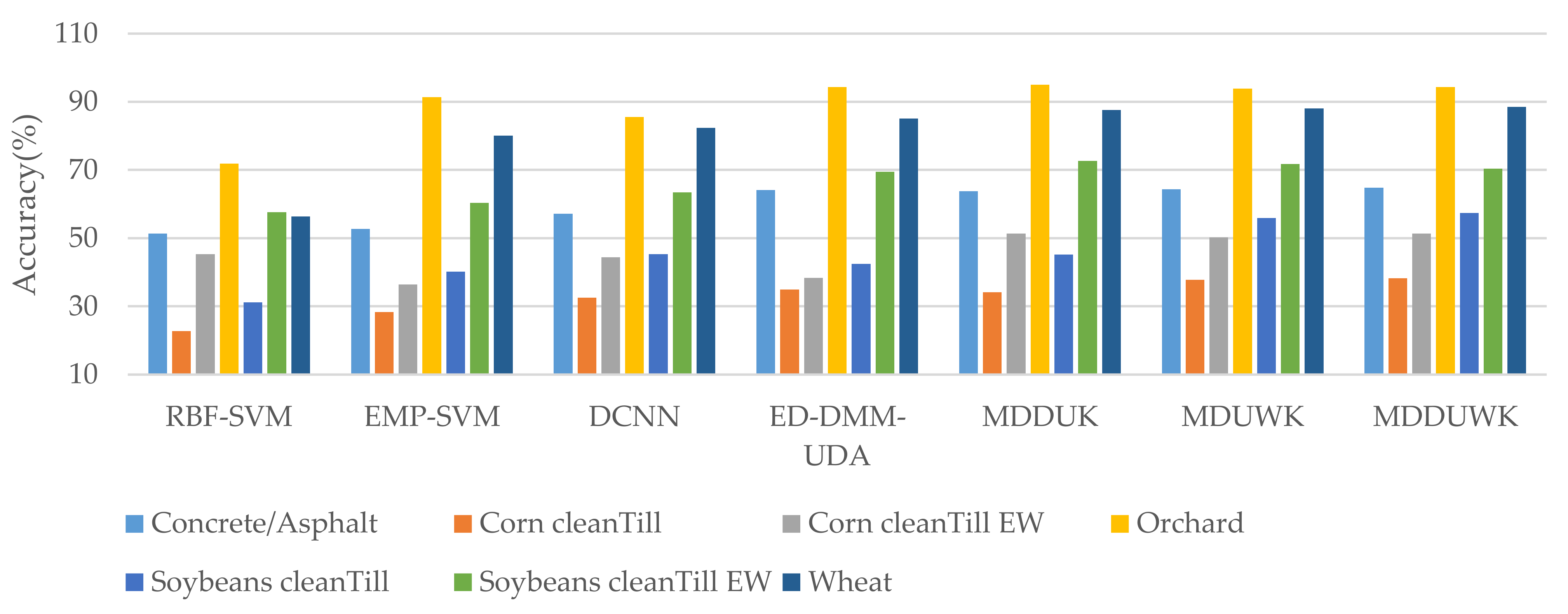
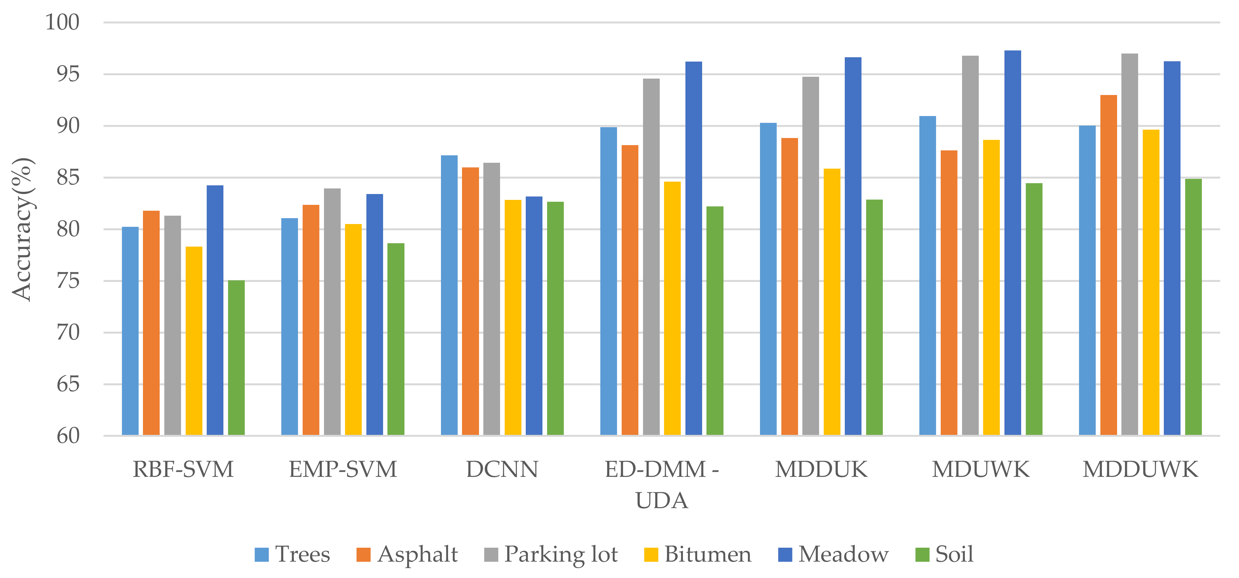
It can be seen from Figure 9 that in the Indiana dataset, the categories of concrete/alpha, orchard and soybeans cleanTill EW of small samples are weighted separately. By comparing MDUWK and ED-DMM-UDA, the accuracy of concrete/alpha and soybeans cleanTill EW is improved by 0.18% and 2.3%. Compared with the improvement of the two types, the reduction by 0.54% in Orchard is acceptable. It can be found from Figure 10 that in the Pavia dataset, the categories of small samples, Parking lot and Bitumen, after using weighting alone, increased by 2.21% and 4.04%, respectively, by comparing MDUWK and ED-DMM-UDA. Therefore, it can be explained that the adaptive weighting method in this paper can effectively handle category unbalanced data. At the same time, MDDUWK obtained 4 best classification accuracy of seven terrain categories of interest in the Indiana dataset and MDDUWK obtains four best classification accuracy of six terrain categories of interest in the Pavia dataset; thus, it can be explained that the proposed algorithm also achieves the best classification effect in each category accuracy.
The running time (training time + test time) of the model is an important evaluation index of the deep learning classification model. Table 6 shows the calculation time consumption of the seven network models. It can be found that when MDDUWK classifies hyperspectral data, the time consumption in Indiana data set is the third and that in Pavia data set is the second, which saves many computing resources. Although MDDUWK spent more time than MDDUK, a slight reduction in time is acceptable compared with the increase of accuracy.
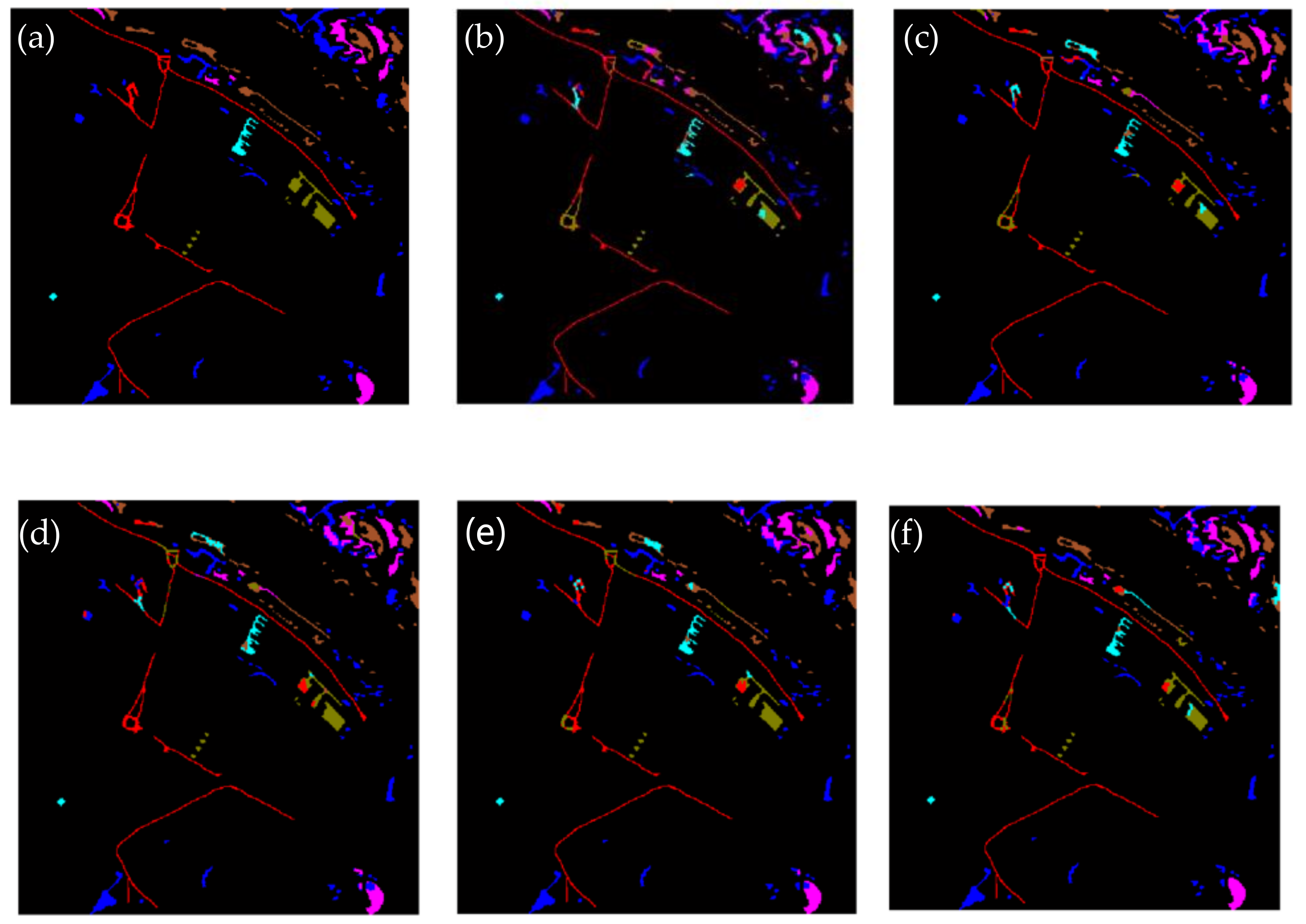
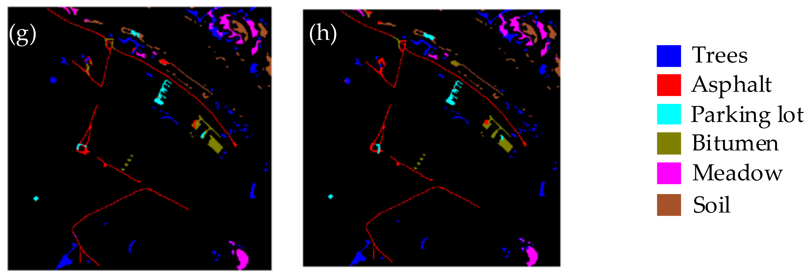
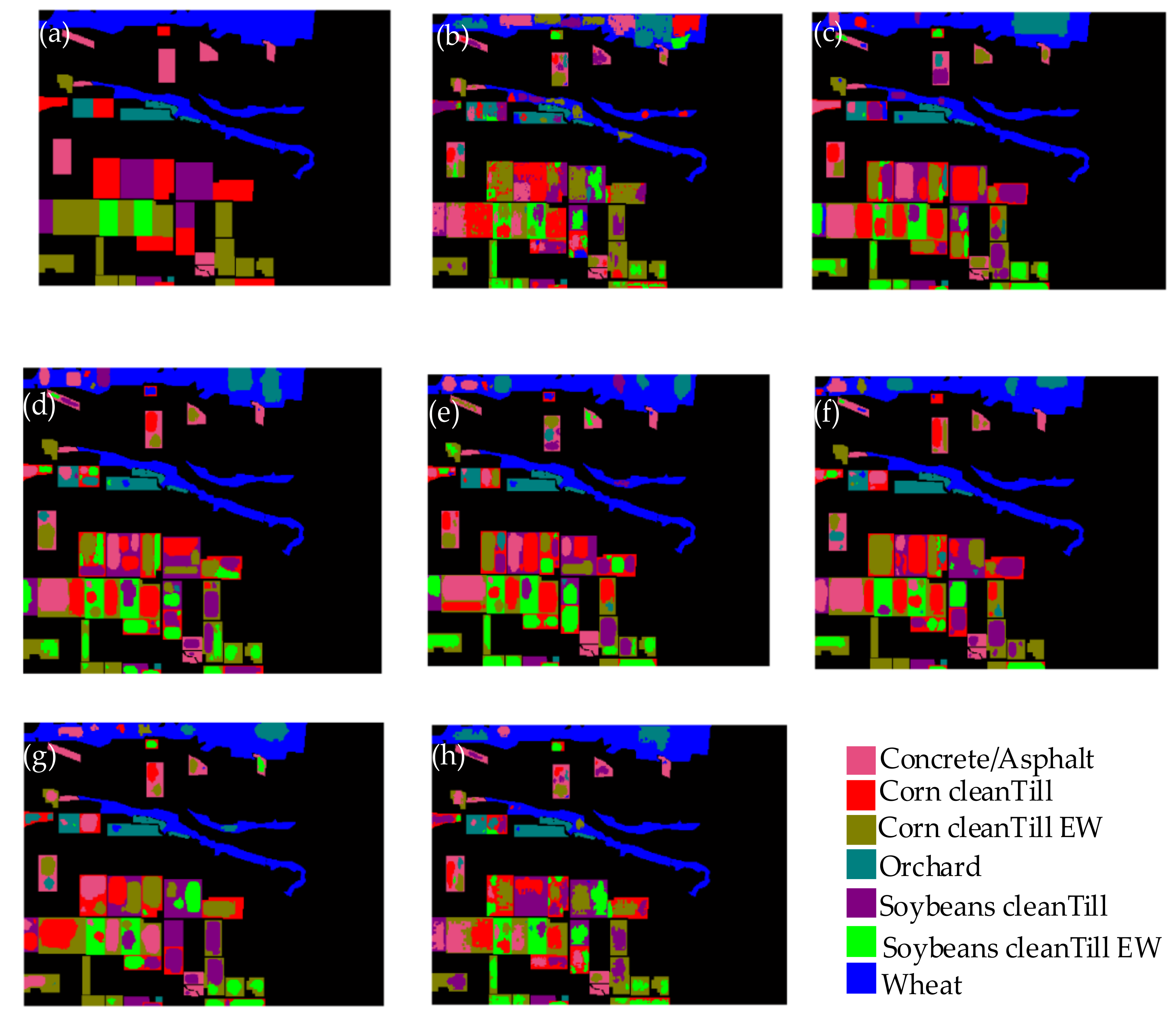
In order to subjectively evaluate the classification effect, Figure 11 and Figure 12 respectively show the truth maps of two HSI data and the pseudo color maps of the classification results of each method. In Figure 11, Asphalt and bitumen both refer to the same black, sticky semi solid or a liquid substance derived from crude oil. However, in regular use, asphalt can also be used as a shortened term for asphalt concrete which is a popular construction composite made up of bitumen and mineral aggregates. Asphalt is called asphaltene. In Figure 12, CleanTill definition is to cultivate by stripping the soil clean of weeds and other harmful growth. EW stands for different longitudes, which are mainly used to distinguish features at different longitudes. Features with different longitudes will have some differences in characteristics. All researchers add EW to identify features more accurately. It can be seen that the method in this paper is closer to the real ground object distribution, and the area of false classification is greatly reduced. Compared with RBF-SVM, EMP-SVM, DCNN, MDDUK and MDUWK, the classification effect is greatly improved.
4. Conclusions
In this paper, a new cross-scene adaptive learning terrain classification model for hyperspectral images is proposed. Based on unsupervised domain adaptive technology, the model introduces depthwise over-parameterized convolution into the embedding model to accelerate the convergence speed of depth convolution neural network. At the same time, learning Manhattan metric distance saves the computational cost of cross-scene model. Finally, a weighted KNN classifier is introduced to enhance the ability of the model to handle data category imbalance problem. In this paper, experiments are carried out on Pavia and Indiana data sets. Compared with other six classification algorithms, this paper has higher classification accuracy and fast model running time. When the number of training samples is 180, overall accuracy on Pavia data set and Indiana data set reaches 90.9% and 65.0%, respectively. The proposed cross-scene classification model in this paper has a better classification effect on hyperspectral images without training samples, and the accuracy has been improved, which can be applied to crop yield estimation, pest detection, atmospheric environment monitoring and other fields. However, the computational cost of the model is still relatively large. Later, the network model will be further lightened to reduce the number of model parameters and improve the training efficiency of the model.
Author Contributions
Conceptualization, A.W. and H.W.; methodology, C.L.; software, C.L. and D.X.; validation, Y.Z. and M.L.; writing—review and editing, C.L. and A.W.; All authors have read and agreed to the published version of the manuscript.
Funding
This work was funded by the National Natural Science Foundation of China under Grant NSFC-61671190.
Data Availability Statement
Acknowledgments
We thank Kaiyuan Jiang and Lanfei Zhao for their valuable comments.
Conflicts of Interest
The authors declare no conflict of interest.
References
- Bo, C.; Lu, H.; Wang, D. Weighted Generalized Nearest Neighbor for Hyperspectral Image Classification. IEEE Access 2017, 5, 1496–1509. [Google Scholar] [CrossRef]
- Huo, L.; Feng, X. Denoising of Hyperspectral remote sensing image based on principal component analysis and dictionary learning. J. Electron. Inf. Technol. 2014, 36, 2723–2729. [Google Scholar]
- Paul, S.; Poliyapram, V.; İmamoğlu, N.; Uto, K.; Nakamura, R.; Kumar, D.N. Canopy Averaged Chlorophyll Content Prediction of Pear Trees Using Convolutional Autoencoder on Hyperspectral Data. IEEE J. Sel. Top. Appl. Earth Obs. Remote. Sens. 2020, 13, 1426–1437. [Google Scholar] [CrossRef]
- Jia, Y.; Feng, Y.; Wang, Z. Hyperspectral compressive sensing recovery via spectrum structure similarity. J. Electron. Inf. Technol. 2014, 36, 1406–1412. [Google Scholar]
- Lacar, F.M.; Lewis, M.M.; Grierson, I.T. Use of hyperspectral imagery for mapping grape varieties in the Barossa Valley, South Australia. In Proceedings of the IGARSS 2001. Scanning the Present and Resolving the Future. Proceedings IEEE 2001 International Geoscience and Remote Sensing Symposium (Cat. No.01CH37217), Sydney, NSW, Australia, 9–13 July 2001; IEEE: Piscataway, NJ, USA, 2001; Volume 6, pp. 2875–2877. [Google Scholar]
- Gowen, A.A. Hyperspectral imaging—An emerging process analytical tool for food quality and safety control. Trends Food Sci.Technol. 2007, 18, 590–598. [Google Scholar] [CrossRef]
- Rubtsova, N.M.; Vinogradovb, A.N.; Kalininc, P.A. Study of Combustion of Hydrogen—Air and Hydrogen-Methane-Air Mixtures over the Palladium Metal Surface Using a Hyperspectral Sensor and High-Speed Color Filming. Russ. J. Phys. Chem. B 2019, 13, 305–312. [Google Scholar] [CrossRef]
- Voloshin, A.E.; Egorov, V.V.; Kalinin, A.P.; Manomenova, V.L. Cluster Control System in Crystallization Setups for Crystal Growth from Low-Temperature Solutions. Crystallogr. Rep. 2019, 64, 363–365. [Google Scholar] [CrossRef]
- Malthus, T.J.; Mumby, P.J. Remote sensing of the coastal zone: An overview and priorities for future research. Int. J. Remote Sens. 2003, 24, 2805–2815. [Google Scholar] [CrossRef]
- Nepobedimyœ, S.P.; Rodionov, I.D.; Vorontsov, D.V. Hyperspectral remote sounding of the ground. Dokl. Phys. 2004, 49, 411–414. [Google Scholar] [CrossRef]
- Tang, H.; Li, Y.; Han, X.; Huang, Q.; Xie, W. A Spatial–Spectral Prototypical Network for Hyperspectral Remote Sensing Image. IEEE Geosci. Remote. Sens. Lett. 2020, 17, 167–171. [Google Scholar] [CrossRef]
- Bo, C.J.; Lu, H.C.; Wang, D. Spectral-spatial K-Nearest Neighbor approach for hyperspectral image classification. Multimed. Tools Appl. 2018, 77, 10419–10436. [Google Scholar] [CrossRef]
- Li, M.; Zhang, N.; Pan, B.; Xie, S.; Wu, X.; Shi, Z. Hyperspectral Image Classification Based on Deep Forest and Spectral-Spatial Cooperative Feature. Proc. ICIG 2017, 10668, 325–336. [Google Scholar]
- LI, W.; PRASAD, S.; FOWLER J., E. Locality-preserving dimensionality reduction and classification for hyperspectral image analysis. IEEE Trans. Geosci. Remote. Sens. 2012, 50, 1185–1198. [Google Scholar] [CrossRef] [Green Version]
- Samadzadegan, F.; Hasani, H.; Schenk, T. Simultaneous feature selection and SVM parameter determination in classification of hyperspectral imagery using Ant Colony Optimization. Remote Sens. 2012, 38, 139–156. [Google Scholar] [CrossRef]
- Jiao, L.; Liang, M.; Chen, H.; Yang, S.; Cao, H.L.X. Deep Fully Convolutional Network-Based Spatial Distribution Prediction for Hyperspectral Image Classification. IEEE Trans. Geosci. Remote. Sens. 2017, 55, 5585–5599. [Google Scholar] [CrossRef]
- Rodionova, I.D.; Rodionova, A.I.; Rodionovaa, I.P. Passage of UV-C, Visible, and Near-Infrared Radiation through the Atmosphere. Russ. J. Phys. Chem. B Focus Phys. 2019, 13, 667–673. [Google Scholar] [CrossRef]
- Liu, X.; Yin, X.; Cai, Y.; Wang, M.; Huang, Z.C.B. Visual Saliency-Based Extended Morphological Profiles for Unsupervised Feature Learning of Hyperspectral Images. IEEE Geosci. Remote. Sens. Lett. 2020, 17, 1963–1967. [Google Scholar] [CrossRef]
- Chen, Y.; Zhu, K.; Zhu, L.; He, X.; Ghamisi, P.; Benediktsson, J.A. Automatic Design of Convolutional Neural Network for Hyperspectral Image Classification. IEEE Trans. Geosci. Remote. Sens. 2019, 57, 7048–7066. [Google Scholar] [CrossRef]
- Chen, Y.; Lin, Z.; Zhao, X.; Wang, G.; Gu, Y. Deep Learning-Based Classification of Hyperspectral Data. IEEE J. Sel. Top. Appl. Earth Obs. Remote. Sens. 2014, 7, 2094–2107. [Google Scholar] [CrossRef]
- Guo, A.J.X.; Zhu, F. A CNN-Based Spatial Feature Fusion Algorithm for Hyperspectral Imagery Classification. IEEE Trans. Geosci. Remote. Sens. 2019, 57, 7170–7181. [Google Scholar] [CrossRef] [Green Version]
- Ge, Z.; Cao, G.; Li, X.; Fu, P. Hyperspectral Image Classification Method Based on 2D–3D CNN and Multibranch Feature Fusion. IEEE J. Sel. Top. Appl. Earth Obs. Remote. Sens. 2020, 13, 5776–5788. [Google Scholar] [CrossRef]
- Zhu, J.; Fang, L.; Ghamisi, P. Deformable Convolutional Neural Networks for Hyperspectral Image Classification. IEEE Geosci. Remote. Sens. Lett. 2018, 15, 1254–1258. [Google Scholar] [CrossRef]
- Yu, C. Hyperspectral Image Classification Method Based on CNN Architecture Embedding with Hashing Semantic Feature. IEEE J. Sel. Top. Appl. Earth Obs. Remote. Sens. 2019, 12, 1866–1881. [Google Scholar] [CrossRef]
- Mei, S.; Ji, J.; Hou, J.; Li, X.; Du, Q. Learning Sensor-Specific Spatial-Spectral Features of Hyperspectral Images via Convolutional Neural Networks. IEEE Trans. Geosci. Remote. Sens. 2017, 55, 4520–4533. [Google Scholar] [CrossRef]
- Pan, B.; Shi, Z.; Xu, X. MugNet: Deep learning for hyperspectral image classification using limited samples. ISPRS J. Photogramm. Remote. Sening 2018, 145, 108–119. [Google Scholar] [CrossRef]
- Sun, H.; Zheng, X.; Lu, X.; Wu, S. Spectral–Spatial Attention Network for Hyperspectral Image Classification. IEEE Trans. Geosci. Remote. Sens. 2020, 58, 3232–3245. [Google Scholar] [CrossRef]
- He, X.; Chen, Y.; Ghamisi, P. Heterogeneous Transfer Learning for Hyperspectral Image Classification Based on Convolutional Neural Network. IEEE Trans. Geosci. Remote. Sens. 2020, 58, 3246–3263. [Google Scholar] [CrossRef]
- Yang, F.S.Y.; Zhang, L.; Xiang, T.; Torr, P.H.; Hospedales, T.M. Learning to compare: Relation network for few-shot learning. In Proceedings of the IEEE Conference on Computer Vision and Pattern Recognition (CVPR), Salt Lake City, UT, USA, 18–23 June 2018; pp. 1199–1208. [Google Scholar] [CrossRef] [Green Version]
- Rao, M.; Tang, P.; Zhang, Z. Spatial–Spectral Relation Network for Hyperspectral Image Classification with Limited Training Samples. IEEE J. Sel. Top. Appl. Earth Obs. Remote. Sens. 2019, 12, 5086–5100. [Google Scholar] [CrossRef]
- Zhang, C.; Yue, J.; Qin, Q. Global Prototypical Network for Few-Shot Hyperspectral Image Classification. IEEE J. Sel. Top. Appl. Earth Obs. Remote. Sens. 2020, 13, 4748–4759. [Google Scholar] [CrossRef]
- Ye, M.; Xu, Y.; Lu, H.; Yan, K.; Qian, Y. Cross-scene feature selection for hyperspectral images based on cross-domain information gain. In Proceedings of the IGARSS 2018–2018 IEEE International Geoscience and Remote Sensing Symposium, Valencia, Spain, 22–27 July 2018; IEEE: Piscataway, NJ, USA, 2018; pp. 4764–4767. [Google Scholar] [CrossRef]
- Ye, M.; Qian, Y.; Zhou, J.; Tang, Y.Y. Dictionary Learning-Based Feature-Level Domain Adaptation for Cross-Scene Hyperspectral Image Classification. IEEE Trans. Geosci. Remote. Sens. 2017, 55, 1544–1562. [Google Scholar] [CrossRef] [Green Version]
- Kemker, R.; Kanan, C. Self-taught feature learning for hyperspectral image classification. IEEE Trans. Geosci. Remote. Sens 2017, 55, 2693–2705. [Google Scholar] [CrossRef]
- Du, B.; Zhang, L.; Tao, D.; Zhang, D. Unsupervised transfer learning for target detection from hyperspectral images. Neurocomputing 2013, 120, 72–82. [Google Scholar] [CrossRef]
- Deng, B.; Jia, S.; Shi, D. Deep Metric Learning-Based Feature Embedding for Hyperspectral Image Classification. IEEE Trans. Geosci. Remote. Sens. 2020, 58, 1422–1435. [Google Scholar] [CrossRef]
- Praveen, B.; Menon, V. Study of Spatial–Spectral Feature Extraction Frameworks With 3D Convolutional Neural Network for Robust Hyperspectral Imagery Classification. IEEE J. Sel. Top. Appl. Earth Obs. Remote. Sens. 2021, 14, 1717–1727. [Google Scholar] [CrossRef]
- Ji, S.; Ma, X.; Wang, W.; Yu, L.; Geng, J.; Wang, H. Hyperspectral Image Classification by Parameters Prediction Networks. In Proceedings of the IGARSS 2019–2019 IEEE International Geoscience and Remote Sensing Symposium, Yokohama, Japan, 28 July–2 August 2019; IEEE: Piscataway, NJ, USA, 2019; pp. 3309–3312. [Google Scholar] [CrossRef]
- Cao, J.; Li, Y.; Sun, M. DO-Conv: Depthwise over-parameterized convolutional layer. arXiv 2020, arXiv:2006.12030. [Google Scholar]
- Song, H.O.; Xiang, Y.; Jegelka, S.; Savarese, S. Deep Metric Learning via Lifted Structured Feature Embedding. In Proceedings of the 2016 IEEE Conference on Computer Vision and Pattern Recognition (CVPR), Las Vegas, NV, USA, 27–30 June 2016; pp. 4004–4012. [Google Scholar] [CrossRef] [Green Version]
- Malkauthekar, M.D. Analysis of euclidean distance and Manhattan Distance measure in face recognition. In Proceedings of the Third International Conference on Computational Intelligence and Information Technology (CIIT 2013), Mumbai, India, 18–19 October 2013; IEEE: Piscataway, NJ, USA, 2013; pp. 503–507. [Google Scholar] [CrossRef]
- Ma, H.; Gou, J.; Wang, X.; Ke, J.; Zeng, S. Sparse Coefficient-Based k-Nearest Neighbor Classification. IEEE Access 2017, 5, 16618–16634. [Google Scholar] [CrossRef]
- Baumgardner, M.F.; Biehl, L.L.; Landgrebe, D.A. 220 Band AVIRIS Hyperspectral Image Data Set: June 12, 1992 AVIRIS Image North-South Flightline. 2015. Available online: https://engineering.purdue.edu/~biehl/MultiSpec/hyperspectral.html (accessed on 30 September 2015).
- Wang, J.; Ye, M.; Xiong, F.; Qian, Y. Cross-Scene Hyperspectral Feature Selection via Hybrid Whale Optimization Algorithm with Simulated Annealing. IEEE J. Sel. Top. Appl. Earth Obs. Remote. Sens. 2021, 14, 2473–2483. [Google Scholar] [CrossRef]
Figure 1.
The proposed cross-scene classification model for hyperspectral image.

Figure 2.
The deep hyperparametric embedding model.

Figure 3.
The depthwise over-parameterized convolution.

Figure 4.
The structure of discriminator model.

Figure 5.
The metric model.

Figure 6.
The weighted K-nearest neighbor.

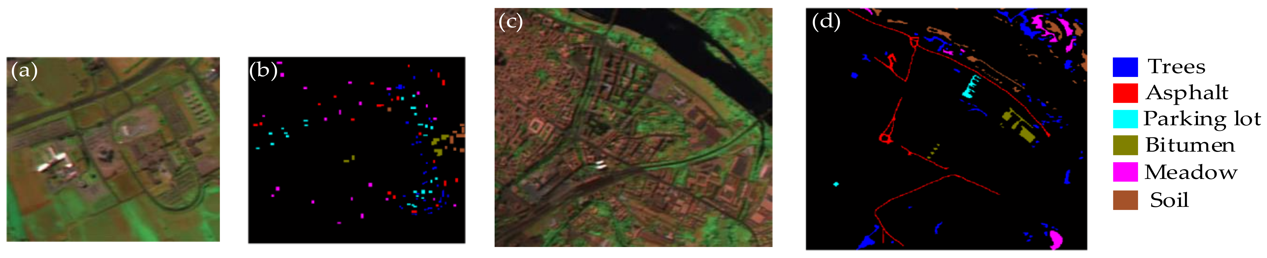
Figure 7.
Indiana dataset. (a) False color image of source scene. (b) Ground truth of source scene. (c) False color image of target scene. (d) Ground truth of target scene.
Figure 7.
Indiana dataset. (a) False color image of source scene. (b) Ground truth of source scene. (c) False color image of target scene. (d) Ground truth of target scene.

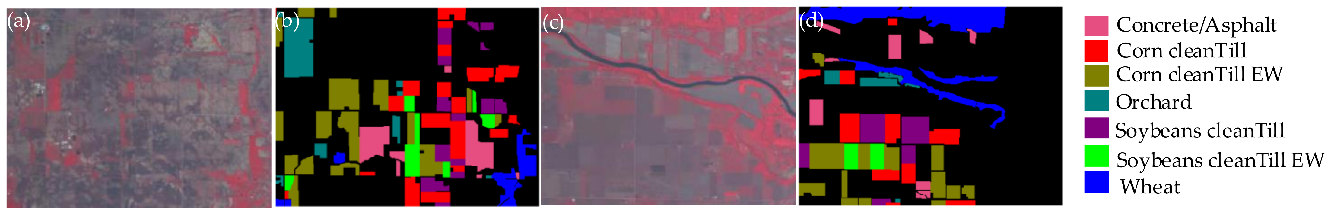
Figure 8.
Pavia dataset (a) False color image of source scene. (b) Ground truth of source scene. (c) False color image of target scene. (d) Ground truth of target scene.
Figure 8.
Pavia dataset (a) False color image of source scene. (b) Ground truth of source scene. (c) False color image of target scene. (d) Ground truth of target scene.

Figure 9.
Different methods’ classification results for each class on Indiana dataset.

Figure 10.
Different methods’ classification results for each class on Pavia dataset.

Figure 11.
Classification results of Pavia dataset. (a) Ground truth; (b) RBF-SVM; (c) EMP-SVM; (d) DCNN; (e) ED-DMM-UDA; (f) MDDUK; (g) MDUWK; (h) MDDUWK.
Figure 11.
Classification results of Pavia dataset. (a) Ground truth; (b) RBF-SVM; (c) EMP-SVM; (d) DCNN; (e) ED-DMM-UDA; (f) MDDUK; (g) MDUWK; (h) MDDUWK.


Figure 12.
Classification results of Indiana dataset. (a) Ground truth; (b) RBF-SVM; (c) EMP-SVM; (d) DCNN; (e) ED-DMM-UDA; (f) MDDUK; (g) MDUWK; (h) MDDUWK.
Figure 12.
Classification results of Indiana dataset. (a) Ground truth; (b) RBF-SVM; (c) EMP-SVM; (d) DCNN; (e) ED-DMM-UDA; (f) MDDUK; (g) MDUWK; (h) MDDUWK.


Table 1.
The weight of category.
| Indiana Scene | Pavia Scene | |||
|---|---|---|---|---|
| Category | Target Scene | Category | Target Scene | |
| C1 | Concrete/Asphalt | 8.24% | Trees | 30.97% |
| C2 | Corn cleanTill | 16.89% | Asphalt | 21.77% |
| C3 | Corn cleanTill EW | 22.41% | Parking lot | 3.67% |
| C4 | Orchard | 4.38% | Bitumen | 8.75% |
| C5 | Soybeans cleanTill | 13.42% | Meadow | 15.99% |
| C6 | Soybeans cleanTill EW | 4.59% | Soil | 18.85% |
| C7 | Wheat | 30.08% | ||
Table 2.
The description Indiana and Pavia datasets.
| Indiana Dataset | Pavia Dataset | |||||
|---|---|---|---|---|---|---|
| Category | Source Scene | Target Scene | Category | Source Scene | Target Scene | |
| C1 | Concrete/Asphalt | 4867 | 2942 | Trees | 266 | 2424 |
| C2 | Corn cleanTill | 9822 | 6029 | Asphalt | 266 | 1704 |
| C3 | Corn cleanTill EW | 11414 | 7999 | Parking lot | 265 | 287 |
| C4 | Orchard | 5106 | 1562 | Bitumen | 206 | 685 |
| C5 | Soybeans cleanTill | 4731 | 4792 | Meadow | 273 | 1251 |
| C6 | Soybeans cleanTill EW | 2996 | 1638 | Soil | 213 | 1475 |
| C7 | Wheat | 3223 | 10739 | |||
Table 3.
Parameters of depthwise hyperparametric embedding model.
| Model | Input | DO-Conv | BN | ReLU | AvgPool | FC Output |
|---|---|---|---|---|---|---|
| Output | Output | |||||
| Parameter | 5 × 5 × nBand | 1 × 1 | Yes | Yes | No | No |
| 5 × 5 × 200 | ||||||
| de | 5 × 5 × 200 | 1 × 1 | Yes | Yes | No | No |
| 5 × 5 × 200 | ||||||
| 5 × 5 × 200 | 1 × 1 | Yes | Yes | No | No | |
| 5 × 5 × 200 | ||||||
| 5 × 5 × 200 | 1 × 1 | Yes | Yes | 5 × 5 | 1 × 128 | |
| 5 × 5 × 200 | 1 × 1 × 200 |
Table 4.
Classification results of Indiana dataset.
| Class | RBF-SVM | EMP-SVM | DCNN | ED-DMM-UDA | MDDUK | MDUWK | MDDUWK |
|---|---|---|---|---|---|---|---|
| C1 C2 C3 C4 C5 C6 C7 | 51.34 22.74 45.32 71.85 31.24 57.62 56.43 | 52.73 28.32 36.43 91.32 40.15 60.42 80.14 | 57.13 32.56 44.39 85.51 45.32 63.47 82.36 | 64.13 34.90 38.41 94.36 42.52 69.47 85.09 | 63.83 34.12 51.36 95.07 45.18 72.68 87.65 | 64.31 37.84 50.26 93.82 55.96 71.77 88.09 | 64.77 38.29 51.33 94.31 57.42 70.43 88.57 |
| OA(%) AA(%) K × 100 time(s) | 45.18 48.08 37.42 70.12 | 53.55 55.64 44.73 215.37 | 57.67 58.68 47.92 149.36 | 58.39 61.27 49.76 86.34 | 62.45 64.27 54.17 84.57 | 64.35 66.01 56.64 84.95 | 65.01 66.45 57.38 84.65 |
Table 5.
Classification results of Pavia dataset.
| Class | RBF-SVM | EMP-SVM | DCNN | ED-DMM-UDA | MDDUK | MDUWK | MDDUWK |
|---|---|---|---|---|---|---|---|
| C1 | 80.24 | 81.06 | 87.13 | 89.86 | 90.30 | 90.95 | 90.02 |
| C2 | 81.78 | 82.34 | 85.99 | 88.14 | 88.82 | 87.62 | 92.99 |
| C3 | 81.32 | 83.94 | 86.43 | 94.57 | 94.76 | 96.78 | 97.00 |
| C4 | 78.31 | 80.51 | 82.84 | 84.59 | 85.85 | 88.63 | 89.62 |
| C5 | 84.24 | 83.41 | 83.16 | 96.21 | 96.65 | 97.29 | 96.26 |
| C6 | 75.06 | 78.65 | 82.65 | 82.21 | 82.85 | 84.45 | 84.88 |
| OA(%) | 80.10 | 81.31 | 84.98 | 88.76 | 89.35 | 90.01 | 90.90 |
| AA(%) | 80.16 | 81.65 | 84.70 | 89.26 | 89.87 | 90.97 | 91.79 |
| K × 100 | 78.32 | 79.13 | 82.15 | 85.83 | 86.58 | 87.41 | 88.52 |
| time(s) | 36.42 | 180.32 | 151.36 | 21.42 | 20.36 | 20.89 | 20.62 |
Table 6.
Computation time comparison when training samples are 180.
| Time(s) | RBF SVM | EMP- SVM | DCNN | ED-DMM- UDA | MDDUK | MDUWK | MDDUWK |
|---|---|---|---|---|---|---|---|
| Indiana | 70.12 | 215.37 | 149.36 | 86.34 | 84.57 | 84.95 | 84.65 |
| Pavia | 36.42 | 180.32 | 151.36 | 21.42 | 20.36 | 20.89 | 20.62 |
Publisher’s Note: MDPI stays neutral with regard to jurisdictional claims in published maps and institutional affiliations. |
© 2021 by the authors. Licensee MDPI, Basel, Switzerland. This article is an open access article distributed under the terms and conditions of the Creative Commons Attribution (CC BY) license (https://creativecommons.org/licenses/by/4.0/).
Share and Cite
MDPI and ACS Style
Wang, A.; Liu, C.; Xue, D.; Wu, H.; Zhang, Y.; Liu, M. Hyperspectral Image Classification Based on Cross-Scene Adaptive Learning. Symmetry 2021, 13, 1878. https://doi.org/10.3390/sym13101878
AMA Style
Wang A, Liu C, Xue D, Wu H, Zhang Y, Liu M. Hyperspectral Image Classification Based on Cross-Scene Adaptive Learning. Symmetry. 2021; 13(10):1878. https://doi.org/10.3390/sym13101878
Chicago/Turabian StyleWang, Aili, Chengyang Liu, Dong Xue, Haibin Wu, Yuxiao Zhang, and Meihong Liu. 2021. "Hyperspectral Image Classification Based on Cross-Scene Adaptive Learning" Symmetry 13, no. 10: 1878. https://doi.org/10.3390/sym13101878
Note that from the first issue of 2016, this journal uses article numbers instead of page numbers. See further details here.