A Comparative Study of the Fractional-Order System of Burgers Equations

Abstract

This paper is related to the fractional view analysis of coupled Burgers equations, using innovative analytical techniques. The fractional analysis of the proposed problems has been done in terms of the Caputo-operator sense. In the current methodologies, first, we applied the Elzaki transform to the targeted problem. The Adomian decomposition method and homotopy perturbation method are then implemented to obtain the series form solution. After applying the inverse transform, the desire analytical solution is achieved. The suggested procedures are verified through specific examples of the fractional Burgers couple systems. The current methods are found to be effective methods having a close resemblance with the actual solutions. The proposed techniques have less computational cost and a higher rate of convergence. The proposed techniques are, therefore, beneficial to solve other systems of fractional-order problems.

1. Introduction

Fractional calculus (FC) has become an important mathematical approach for explaining non-local behavioural models. Fractional derivatives have mathematically interpreted many physical problems in recent decades; these representations have produced excellent results in real-world modelling issues. Coimbra, Riemann–Liouville, Riesz, Weyl, Hadamard, Liouville–Caputo, Grunwald–Letnikov, Caputo–Fabrizio, Atangana–Baleanu, among others, gave many basic definitions of fractional operators [1,2]. A wide variety of non-linear equations have been developed and commonly implemented in numerous non-linear physical sciences such as biology, chemistry, applied mathematics and various branches of physics such as plasma physics, condensed matter physics, fluid mechanics, field theory, and non-linear optics over the past few years. The exact result of non-linear equations plays a vital role in deciding the characteristics and behaviour of physical processes. A differential equation symmetry is a transformation that makes the differential equation invariant. The existence of such symmetries may aid in the solution of the differential equation. A scheme of differential equations line symmetry is a continous symmetry of a scheme of differential equations. Solving a linked set of ordinary differential equations can reveal symmetries. It is sometimes easier to solve these equations than it is to solve the original differential equations. The symmetry structure of the system consists of integer partial differential equations and fractional-order partial differential equations with the fractional Caputo derivative. Many effective techniques have been used to solved nonlinear FPDEs, for example, the homotopy perturbation transformation technique [3,4], the homotopy analysis transformation technique [5,6], reduced differential transformation technique [7,8], the finite element method [9], the finite difference method [10], and so on.

Harry Bateman first introduced the Burgers equation in 1915 [11], and subsequently called it the Burgers equation [12]. The Burgers equation has several implementations in engineering and science, particularly in problems that have non-linear equations in their form. It is one of the most basic tools for defining the non-linear phenomenon of dispersion and diffusion, such as approximation theory of flow, shock wave theory, dynamics of soil in water, unsaturated oil, seismology and cosmology, and debris flow wave with non-linear kinematics [13]. With the aid of the Burgers equations, the analytical and numerical methods can be understood. Many mathematical techniques are used to find the burgers equations, such as Adomian Pade technique [14], differential transformation method [15], tanh-function method [16], homotopy analysis method [17], natural decomposition method [18] and Chebyshev wavelet method [19].

The homotopy perturbation method (HPM), first suggested by the Chinese scientist J.H. He plays a crucial role in 1998 [20]. Because of the way it approaches the system, it does not require any linearization or discrimination. This method is equitable, effective, and efficient, as it reduces an unconditioned matrix, complicated integrals and infinite series. This technique does not require a particular problem parameter. Tarig Elzaki introduced the Ezaki Transform (E.T.) in 2010. E.T. is a Sumudu and Laplace transform that has been modified. Absolute differential equations with variable coefficients cannot be solved by Laplace and Sumudu transformation when E.T is used [21,22,23]. The homotopy perturbation transformation method (HPTM) combines the Elzaki transformation and the homotopy perturbation method. Numerous researchers have used HPTM to solve various models, such as Navier–Stokes equations [24], heat-like equations [25], gas dynamic equation [26], hyperbolic equation and Fisher’s equation [27]. The Elzaki decomposition technique, which is the mixture of the Elzaki transformation introduces by Elzaki [28] and the Adomian decomposition technique [29,30,31]. The transformation of Elzaki is well-known for its efficiency in solving linear ordinary differential equations, linear partial differential equations and integral equations as seen in [32,33,34].

In the current study, we implemented HPTM and EDM to analyze the fractional-order system of Burgers equations. The methodology of the proposed techniques is effortless and straightforward. The accuracy is determined in terms of absolute error. The solutions have shown the present techniques have the desired accuracy as compare to other analytical techniques.

2. Preliminary Concepts

Definition 1.

The fractional-order Caputo derivative of $h(\Im )$, $h\in C_{-1}^{\omega }$, $\omega \in N$, $\omega >0$, is given as

$$D^{\alpha }h(\Im )=I^{\omega -\alpha }{D}^{\omega }h(\Im )=\frac{1}{\mathrm{\Gamma }(\omega -\alpha )}{\int }_0^{\Im }{(\Im -\zeta )}^{\omega -\alpha -1}{h}^{\omega }\left(\zeta \right)d\zeta ,where\omega -1<\alpha \le \omega .$$

Definition 2.

The fractional-order Caputo derivative of Elzaki transform is define as

$$E\left[D_{\Im }^{\alpha }h(\Im )\right]=s^{\alpha }E\left[h(\Im )\right]-\sum _{k=0}^{\omega -1}{s}^{2-\alpha +k}{h}^{\left(k\right)}\left(0\right),where\omega -1<\alpha <\omega .$$

Definition 3.

The fractional-order Riemann–Liouville of integral $\alpha >0$, of a function $h\in C_{\omega }$, is given as

$$\begin{array}{cc}\hfill & J^{\alpha }h\left(\zeta \right)=\frac{1}{\mathrm{\Gamma }\left(\alpha \right)}{\int }_0^{\zeta }{(\zeta -\Im )}^{\alpha -1}h(\Im )\partial \Im ,\alpha ,\zeta >0,\hfill \end{array}$$

Basic properties:

For $h\in C_{\omega }$, $\alpha ,\beta \ge 0and\gamma >-1$

$$\begin{array}{cc}\hfill & J^{\alpha }{J}^{\beta }h\left(\zeta \right)=j^{\alpha +\beta }h\left(\zeta \right),\hfill \\ \hfill & J^{\alpha }{J}^{\beta }h\left(\zeta \right)=J^{\beta }{J}^{\alpha }h\left(\zeta \right),\hfill \\ \hfill & J^{\gamma }{\zeta }^{\alpha }=\frac{\mathrm{\Gamma }(\alpha +1)}{(\gamma +\alpha +1)}{\zeta }^{\gamma +\alpha }.\hfill \end{array}$$

Basic Concept of Elzaki Transformation

The Elzaki transformation is a new transformation described for functions of exponential order. We recognize functions in the set $\mathbb{A}$, described as:

$$\mathbb{A}=\{h(\Im ):\exists |M,k_1,k_2>0,|h(\Im )|<M{e}^{\frac{|\Im |}{k_j}},if(\Im )\in {(-1)}^j\times [0,\infty )\}.$$

For a given function in the set, the constant M must be a finite number, and the constants $k_1$ and $k_2$ must be finite or infinite. The Elzaki transformation, as described by the integral equation

$$E\left[h(\Im )\right]=\mathfrak{T}\left(s\right)=s{\int }_0^{\infty }h(\Im )e^{\frac{-\Im }{s}}d\Im ,\Im \ge 0,k_1\le s\le k_2.$$

We can obtain the basic solutions

$$\begin{array}{cc}\hfill & E\left[{\Im }^n\right]=n!s^{n+2},\hfill \\ \hfill & E\left[h^{\prime }(\Im )\right]=\frac{\mathfrak{T}\left(s\right)}{s}-sh\left(0\right),\hfill \\ \hfill & E\left[h^{″}(\Im )\right]=\frac{\mathfrak{T}\left(s\right)}{s^2}-h\left(0\right)-s{h}^{\prime }\left(0\right),\hfill \\ \hfill & E\left[h^{\left(n\right)}(\Im )\right]=\frac{\mathfrak{T}\left(s\right)}{s^n}-\sum _{k=0}^{n-1}{s}^{2-n+k}{h}^{\left(k\right)}\left(0\right).\hfill \end{array}$$

Definition 4.

The inverse Elzaki transform is given as

$$E^{-1}\left[\mathfrak{T}\left(s\right)\right]=h(\Im )=\frac{1}{2\pi \iota }{\int }_{\alpha -\iota \infty }^{\alpha +\iota \infty }h\left(\frac{1}{s}\right)e^{s\Im }sds=\mathrm{\Sigma }residuesofh\left(\frac{1}{s}\right)e^{s\Im }s.$$

The inverse Elzaki transform of some of the functions are given by

$$\begin{array}{cc}\hfill & •E^{-1}\left\{s^n\right\}=\frac{{\Im }^{n-2}}{(n-2)!},n=2,3,4,\cdots .\hfill \\ \hfill & •E^{-1}\left(\frac{s^2}{1-as}\right)=e^{a\Im }\hfill \\ \hfill & •E^{-1}\left(\frac{s^3}{1+a^2{s}^2}\right)=\frac{1}{a}sina\Im \hfill \\ \hfill & •E^{-1}\left(\frac{s^2}{1+a^2{s}^2}\right)=\frac{1}{a}cosa\Im \hfill \end{array}$$

Theorem 1.

If $\mathfrak{T}\left(s\right)$ is the Elzaki transformation of $h(\Im )$, one can take into consideration the Elzaki transformation of the Riemann–Liouville derivative as follows:

$$E\left[D^{\alpha }h(\Im )\right]=s^{-\alpha }\left[\mathfrak{T}\left(s\right)-\sum _{\omega =1}^n\left\{D^{\alpha -k}h\left(0\right)\right\}\right];-1<n-1\le \alpha <n.$$

Proof. 

The Laplace transformation

$$h^{\prime }(\Im )=\frac{d}{d\Im }h(\Im ),$$

$$L\left[D^{\alpha }h(\Im )\right]=s^{\alpha }\mathfrak{T}\left(s\right)-\sum _{\omega =0}^{n-1}{s}^{\omega }\left[D^{\alpha -\omega -1}h\left(0\right)\right],$$

$$=s^{\alpha }\mathfrak{T}\left(s\right)-\sum _{\omega =0}^{n-1}{s}^{\omega -1}\left[D^{\alpha -\omega }h\left(0\right)\right]=s^{\alpha }\mathfrak{T}\left(s\right)-\sum _{\omega =0}^{n-1}{s}^{\omega -2}\left[D^{\alpha -\omega }h\left(0\right)\right],$$

$$=s^{\alpha }\mathfrak{T}\left(s\right)-\sum _{\omega =0}^{n-1}\frac{1}{s^{-\omega +2}}\left[D^{\alpha -\omega }h\left(0\right)\right]=s^{\alpha }\mathfrak{T}\left(s\right)-\sum _{\omega =0}^{n-1}\frac{1}{s^{\alpha -\omega +2-\alpha }}\left[D^{\alpha -\omega }h\left(0\right)\right],$$

$$=s^{\alpha }\mathfrak{T}\left(s\right)-\sum _{\omega =0}^{n-1}{s}^{\alpha }\frac{1}{s^{\alpha -\omega +2}}\left[D^{\alpha -\omega }h\left(0\right)\right],$$

$$L\left[D^{\alpha }h(\Im )\right]=s^{\alpha }\left[\mathfrak{T}\left(s\right)-\sum _{\omega =0}^{n-1}{\left(\frac{1}{s}\right)}^{\alpha -\omega +2}\left[D^{\alpha -\omega }h\left(0\right)\right]\right].$$

Therefore, when we put $\frac{1}{s}$ for $s^2$, the Elzaki transformation of fractional-order of $h(\Im )$ is as below:

$$E\left[D^{\alpha }h(\Im )\right]=s^{-\alpha }\left[\mathfrak{T}\left(s\right)-\sum _{\omega =0}^n{s}^{\alpha -\omega +2}\left[D^{\alpha -\omega }h\left(0\right)\right]\right].$$

□

3. The General Methodology of HPTM

In this section, the HPTM for the solution of fractional partial differential equations [35,36]

$$\begin{array}{cc}\hfill & D_{\Im }^{\alpha }u(\xi ,\zeta ,\Im )+Mu(\xi ,\zeta ,\Im )+Nu(\xi ,\zeta ,\Im )=h(\xi ,\zeta ,\Im ),\Im >0,0<\alpha \le 1,\hfill \end{array}$$

(1)

the initial condition is

$$\begin{array}{c}\hfill u(\zeta ,0)=h\left(\zeta \right).\end{array}$$

(2)

M is linear and N non-linear functions. Using the Elzaki transform of Equation (1)

$$\begin{array}{cc}\hfill & E[D_{\Im }^{\alpha }u(\xi ,\zeta ,\Im )+Mu(\xi ,\zeta ,\Im )+Nu(\xi ,\zeta ,\Im )]=E\left[h(\xi ,\zeta ,\Im )\right],\Im >0,0<\alpha \le 1,\hfill \\ \hfill & u(\xi ,\zeta ,\Im )=s^{2}h\left(\zeta \right)+s^{\alpha }E\left[h(\xi ,\zeta ,\Im )\right]-s^{\alpha }E[Mu(\xi ,\zeta ,\Im )+Nu(\xi ,\zeta ,\Im )].\hfill \end{array}$$

(3)

Now, by applying inverse transformation, we get

$$u(\xi ,\zeta ,\Im )=E^{-1}\left[s^{2}h\left(\zeta \right)+s^{\alpha }E\left[h(\xi ,\zeta ,\Im )\right]\right]-E^{-1}\left[s^{\alpha }E\{Mu(\xi ,\zeta ,\Im )+Nu(\xi ,\zeta ,\Im )\}\right],$$

(4)

where

$$u(\xi ,\zeta ,\Im )=h\left(\zeta \right)+E^{-1}\left[s^{\alpha }E\left[h(\xi ,\zeta ,\Im )\right]\right]-E^{-1}\left[s^{\alpha }E\{Mu(\xi ,\zeta ,\Im )+Nu(\xi ,\zeta ,\Im )\}\right],$$

(5)

The perturbation methodology in based on power series with parameter p is now described as

$$u(\xi ,\zeta ,\Im )=\sum _{k=0}^{\infty }{p}^k{u}_k(\xi ,\zeta ,\Im ),$$

(6)

where perturbation term p and $p\in [0,1]$.

The non-linear functions can be defined as

$$Nu(\xi ,\zeta ,\Im )=\sum _{k=0}^{\infty }{p}^k{H}_k\left(u_k\right),$$

(7)

where $H_{\omega }$ are He’s polynomials of $u_0,u_1,u_2,\cdots ,u_{\omega },$ and can be determined as

$$H_{\omega }(u_0,u_1,\cdots ,u_{\omega })=\frac{1}{\omega !}\frac{{\partial }^{\omega }}{\partial p^{\omega }}{\left[N\left(\sum _{k=0}^{\infty }{p}^k{u}_k\right)\right]}_{p=0},\omega =0,1,2\cdots .$$

(8)

putting Equations (7) and (8) in Equation (4), we have

$$\sum _{k=0}^{\infty }{p}^k{u}_k(\xi ,\zeta ,\Im )=h\left(\zeta \right)+E^{-1}\left[s^{\alpha }E\left[h(\xi ,\zeta ,\Im )\right]\right]-p\times \left[E^{-1}\{s^{\alpha }E\{M\sum _{k=0}^{\infty }{p}^k{u}_k(\xi ,\zeta ,\Im )+\sum _{k=0}^{\infty }{p}^k{H}_k\left(u_k\right)\}\}\right].$$

(9)

Both sides comparison coefficient of p, we have

$$\begin{array}{cc}\hfill & p^0:u_0(\xi ,\zeta ,\Im )=h\left(\zeta \right)+E^{-1}\left[s^{\alpha }E\left[h(\xi ,\zeta ,\Im )\right]\right],\hfill \\ \hfill & p^1:u_1(\xi ,\zeta ,\Im )=E^{-1}\left[s^{\alpha }E(M{u}_0(\xi ,\zeta ,\Im )+H_0\left(u\right))\right],\hfill \\ \hfill & p^2:u_2(\xi ,\zeta ,\Im )=E^{-1}\left[s^{\alpha }E(M{u}_1(\xi ,\zeta ,\Im )+H_1\left(u\right))\right],\hfill \\ \hfill & ⋮\hfill \\ \hfill & p^k:u_k(\xi ,\zeta ,\Im )=E^{-1}\left[s^{\alpha }E(M{u}_{k-1}(\xi ,\zeta ,\Im )+H_{k-1}\left(u\right))\right],k>0,k\in N.\hfill \end{array}$$

(10)

$$u(\xi ,\zeta ,\Im )=\underset{M\to \infty }{lim}\sum _{k=1}^M{u}_k(\xi ,\zeta ,\Im ).$$

(11)

4. The Methodology of EDM

Consider the general procedure of EDM to solve the fractional partial differential equation.

$$D_{\Im }^{\alpha }u(\xi ,\zeta ,\Im )+Lu(\xi ,\zeta ,\Im )+Nu(\xi ,\zeta ,\Im )=q(\xi ,\zeta ,\Im ),\xi ,\zeta ,\Im \ge 0,\omega -1<\alpha <\omega ,$$

(12)

with the initial condition

$$u(\xi ,\zeta ,0)=k\left(\xi \right),$$

(13)

Where is $D_{\Im }^{\alpha }=\frac{{\partial }^{\alpha }}{\partial {\Im }^{\alpha }}$ the Caputo fractional derivative of order $\alpha$, L and N are linear and non-linear functions, respectively and q is source function.

Applying the Elzaki transform to Equation (12),

$$\mathtt{E}\left[D^{\alpha }u(\xi ,\zeta ,\Im )\right]+\mathtt{E}\left[Lu(\xi ,\zeta ,\Im )+Nu(\xi ,\zeta ,\Im )\right]=\mathtt{E}\left[q(\xi ,\zeta ,\Im )\right].$$

(14)

Using the differentiation property, we get

$$\frac{1}{s^{\alpha }}\mathtt{E}\left[u(\xi ,\zeta ,\Im )\right]-s^{2-\alpha }u(\xi ,\zeta ,0)=\mathtt{E}\left[q(\xi ,\zeta ,\Im )\right]-\mathtt{E}\left[Lu(\xi ,\zeta ,\Im )+Nu(\xi ,\zeta ,\Im )\right],$$

$$\mathtt{E}\left[u(\xi ,\zeta ,\Im )\right]=s^{2}u(\xi ,\zeta ,0)+s^{\alpha }\mathtt{E}\left[q(\xi ,\zeta ,\Im )\right]-s^{\alpha }\mathtt{E}\left[Lu(\xi ,\zeta ,\Im )+Nu(\xi ,\zeta ,\Im )\right],$$

Now, $u(\xi ,0)=k\left(\xi \right)$

$$\mathtt{E}\left[u(\xi ,\zeta ,\Im )\right]=s^{2}k\left(\xi \right)+s^{\alpha }\mathtt{E}\left[q(\xi ,\zeta ,\Im )\right]-s^{\alpha }\mathtt{E}\left[Lu(\xi ,\zeta ,\Im )+Nu(\xi ,\zeta ,\Im )\right].$$

(15)

The infinite series solution of $u(\xi ,\zeta ,\Im )$

$$u(\xi ,\zeta ,\Im )=\sum _{\omega =0}^{\infty }{u}_{\omega }(\xi ,\zeta ,\Im ),$$

(16)

The nonlinear terms of N to solve with the help of Adomian polynomials is defined as

$$Nu(\xi ,\zeta ,\Im )=\sum _{\omega =0}^{\infty }{A}_{\omega },$$

(17)

$$A_{\omega }=\frac{1}{\omega !}{\left[\frac{d^{\omega }}{d{\lambda }^{\omega }}\left[N\sum _{\omega =0}^{\infty }\left({\lambda }^{\omega }{u}_{\omega }\right)\right]\right]}_{\lambda =0},\omega =0,1,2\cdots$$

(18)

Putting Equation (16) and Equation (17) into (15),

$$\mathtt{E}\left[\sum _{\omega =0}^{\infty }{u}_{\omega +1}(\xi ,\zeta ,\Im )\right]=s^{2}k\left(\xi \right)+s^{\alpha }\mathtt{E}\left[q(\xi ,\zeta ,\Im )\right]-s^{\alpha }\mathtt{E}\left[L\sum _{\omega =0}^{\infty }{u}_{\omega }(\xi ,\zeta ,\Im )+\sum _{\omega =0}^{\infty }{A}_{\omega }\right].$$

(19)

Now using EDM, we have

$$\mathtt{E}\left[u_0(\xi ,\zeta ,\Im )\right]=s^{2}k\left(\xi \right)+s^{\alpha }\mathtt{E}\left[q(\xi ,\zeta ,\Im )\right],$$

(20)

Generally, we can write

$$\mathtt{E}\left[u_{\omega +1}(\xi ,\zeta ,\Im )\right]=-s^{\alpha }\mathtt{E}\left[L{u}_{\omega }(\xi ,\zeta ,\Im )+A_{\omega }\right],\omega \ge 1.$$

(21)

Implemented the inverse Elzaki transform of Equations (20) and (21), we get

$$u_0(\xi ,\zeta ,\Im )=k\left(\xi \right)+{\mathtt{E}}^{-1}\left[s^{\alpha }\mathtt{E}\left[q(\xi ,\zeta ,\Im )\right]\right]$$

$$u_{\omega +1}(\xi ,\zeta ,\Im )=-{\mathtt{E}}^{-1}\left[s^{\alpha }\mathtt{E}\left[L{u}_{\omega }(\xi ,\zeta ,\Im )+A_{\omega }\right]\right].$$

(22)

Example 1.

Consider the fractional-order system of Burgers equations

$$\begin{array}{cc}\hfill D_{\Im }^{\alpha }u& +u\frac{\partial u}{\partial \xi }+v\frac{\partial u}{\partial \zeta }=\frac{1}{Re}\left[\frac{{\partial }^{2}u}{\partial {\xi }^2}+\frac{{\partial }^{2}u}{\partial {\zeta }^2}\right],\hfill \\ \hfill D_{\Im }^{\beta }v& +u\frac{\partial v}{\partial \xi }+v\frac{\partial v}{\partial \zeta }=\frac{1}{Re}\left[\frac{{\partial }^{2}v}{\partial {\xi }^2}+\frac{{\partial }^{2}v}{\partial {\zeta }^2}\right],0<\alpha ,\beta \le 1,\hfill \end{array}$$

(23)

with initial conditions

$$\begin{array}{cc}\hfill u(\xi ,\zeta ,0)& =\frac{3}{4}-\frac{1}{4(1+exp((Re/32)-4\xi +4\zeta \left)\right)},\hfill \\ \hfill v(\xi ,\zeta ,0)& =\frac{3}{4}+\frac{1}{4(1+exp((Re/32)-4\xi +4\zeta \left)\right)}.\hfill \end{array}$$

(24)

Re denotes the Reynolds number. Now, by applying$ET$to Equation (23), we obtain the following outcome

$$\begin{array}{cc}\hfill E\left[D_{\Im }^{\alpha }u(\xi ,\zeta ,\Im )\right]& =-E\left\{u\frac{\partial u}{\partial \xi }\right\}-E\left\{v\frac{\partial u}{\partial \zeta }\right\}+\frac{1}{Re}\left[E\left\{\frac{{\partial }^{2}u}{\partial {\xi }^2}\right\}+E\left\{\frac{{\partial }^{2}u}{\partial {\zeta }^2}\right\}\right],\hfill \\ \hfill E\left[D_{\Im }^{\beta }v(\xi ,\zeta ,\Im )\right]& =-E\left\{u\frac{\partial v}{\partial \xi }\right\}-E\left\{v\frac{\partial v}{\partial \zeta }\right\}+\frac{1}{Re}\left[E\left\{\frac{{\partial }^{2}v}{\partial {\xi }^2}\right\}+E\left\{\frac{{\partial }^{2}v}{\partial {\zeta }^2}\right\}\right].\hfill \end{array}$$

(25)

Define the non-linear operator as

$$\begin{array}{cc}\hfill \frac{1}{s^{\alpha }}E\left[u(\xi ,\zeta ,\Im )\right]-s^{2-\alpha }u(\xi ,\zeta ,0)& =E\left[-u\frac{\partial u}{\partial \xi }-v\frac{\partial u}{\partial \zeta }+\frac{1}{Re}\left(\frac{{\partial }^{2}u}{\partial {\xi }^2}+\frac{{\partial }^{2}u}{\partial {\zeta }^2}\right)\right],\hfill \\ \hfill \frac{1}{s^{\beta }}E\left[v(\xi ,\zeta ,\Im )\right]-s^{2-\beta }v(\xi ,\zeta ,0)& =E\left[-u\frac{\partial v}{\partial \xi }-v\frac{\partial v}{\partial \zeta }+\frac{1}{Re}\left(\frac{{\partial }^{2}u}{\partial {\xi }^2}+\frac{{\partial }^{2}u}{\partial {\zeta }^2}\right)\right].\hfill \end{array}$$

(26)

By the above equation, we get

$$\begin{array}{cc}\hfill E\left[u\right(\xi ,\zeta ,\Im \left)\right]& =s^2\left[\frac{3}{4}-\frac{1}{4(1+exp((Re/32)-4\xi +4\zeta \left)\right)}\right]+s^{\alpha }\left[-u\frac{\partial u}{\partial \xi }-v\frac{\partial u}{\partial \zeta }+\frac{1}{Re}\left(\frac{{\partial }^{2}u}{\partial {\xi }^2}+\frac{{\partial }^{2}u}{\partial {\zeta }^2}\right)\right],\hfill \\ \hfill E\left[v\right(\xi ,\zeta ,\Im \left)\right]& =s^2\left[\frac{3}{4}+\frac{1}{4(1+exp((Re/32)-4\xi +4\zeta \left)\right)}\right]+s^{\beta }\left[-u\frac{\partial v}{\partial \xi }-v\frac{\partial v}{\partial \zeta }+\frac{1}{Re}\left(\frac{{\partial }^{2}v}{\partial {\xi }^2}+\frac{{\partial }^{2}v}{\partial {\zeta }^2}\right)\right].\hfill \end{array}$$

(27)

Apply inverse $ET$ on Equation (27) and then reduces to

$$\begin{array}{cc}\hfill u(\xi ,\zeta ,\Im )& =\left[\frac{3}{4}-\frac{1}{4(1+exp((Re/32)-4\xi +4\zeta \left)\right)}\right]+E^{-1}\left[s^{\alpha }\left\{-u\frac{\partial u}{\partial \xi }-v\frac{\partial u}{\partial \zeta }+\frac{1}{Re}\left(\frac{{\partial }^{2}u}{\partial {\xi }^2}+\frac{{\partial }^{2}u}{\partial {\zeta }^2}\right)\right\}\right],\hfill \\ \hfill v(\xi ,\zeta ,\Im )& =\left[\frac{3}{4}+\frac{1}{4(1+exp((Re/32)-4\xi +4\zeta \left)\right)}\right]+E^{-1}\left[s^{\beta }\left\{-u\frac{\partial v}{\partial \xi }-v\frac{\partial v}{\partial \zeta }+\frac{1}{Re}\left(\frac{{\partial }^{2}v}{\partial {\xi }^2}+\frac{{\partial }^{2}v}{\partial {\zeta }^2}\right)\right\}\right].\hfill \end{array}$$

(28)

Now we implement HPM

$$\begin{array}{cc}\hfill \sum _{\omega =0}^{\infty }{p}^{\omega }{u}_{\omega }(\xi ,\zeta ,\Im )=& \left[\frac{3}{4}-\frac{1}{4(1+exp((Re/32)-4\xi +4\zeta \left)\right)}\right]\hfill \\ & +p\left[E^{-1}\left\{s^{\alpha }E\left(\left(\sum _{\omega =0}^{\infty }{p}^{\omega }\frac{1}{Re}\left(\frac{{\partial }^2{u}_{\omega }}{\partial {\xi }^2}+\frac{{\partial }^2{u}_{\omega }}{\partial {\zeta }^2}\right)\right)+\left(\sum _{\omega =0}^{\infty }{p}^{\omega }{H}_{\omega }\left(u\right)\right)\right)\right\}\right].\hfill \\ \hfill \sum _{\omega =0}^{\infty }{p}^{\omega }{v}_{\omega }(\xi ,\zeta ,\Im )=& \left[\frac{3}{4}+\frac{1}{4(1+exp((Re/32)-4\xi +4\zeta \left)\right)}\right]\hfill \\ & +p\left[E^{-1}\left\{s^{\beta }E\left(\left(\sum _{\omega =0}^{\infty }{p}^{\omega }\frac{1}{Re}\left(\frac{{\partial }^2{v}_m}{\partial {\xi }^2}+\frac{{\partial }^2{v}_{\omega }}{\partial {\zeta }^2}\right)\right)+\left(\sum _{\omega =0}^{\infty }{p}^{\omega }{H}_{\omega }\left(v\right)\right)\right)\right\}\right].\hfill \end{array}$$

(29)

With the help of He’s polynomials $H_{\omega }\left(u\right)$ and $H_{\omega }\left(v\right)$, the nonlinear terms can be found

$${\mathrm{\Sigma }}_{\omega =0}^{\infty }{p}^{\omega }{H}_{\omega }\left(u\right)=-u{u}_{\xi }-v{u}_{\zeta },{\mathrm{\Sigma }}_{\omega =0}^{\infty }{p}^{\omega }{H}_{\omega }\left(v\right)=-u{v}_{\xi }-v{v}_{\zeta }.$$

(30)

He’s polynomials are defined as

$$\begin{array}{cc}\hfill H_0\left(u\right)& =-u_0{u_0}_{\xi }-v_0{u_0}_{\zeta },H_0\left(v\right)=-u_0{v_0}_{\xi }-v_0{v_0}_{\zeta },\hfill \\ \hfill H_1\left(u\right)& =-(u_0{u_1}_{\xi }+u_1{u_0}_{\xi })-(v_0{u_1}_{\zeta }+v_1{u_0}_{\zeta }),H_1\left(v\right)=-(u_0{v_1}_{\xi }+u_1{v_0}_{\xi })-(v_0{v_1}_{\zeta }+v_1{v_0}_{\zeta }),\hfill \\ \hfill ⋮\end{array}$$

Comparing p-like coefficients, we get

$$\begin{array}{cc}\hfill p^0:u_0(\xi ,\zeta ,\Im )=& \frac{3}{4}-\frac{1}{4(1+exp((Re/32)-4\xi +4\zeta \left)\right)},\hfill \\ \hfill p^0:v_0(\xi ,\zeta ,\Im )=& \frac{3}{4}+\frac{1}{4(1+exp((Re/32)-4\xi +4\zeta \left)\right)},\hfill \end{array}$$

$$\begin{array}{cc}\hfill p^1:u_1(\xi ,\zeta ,\Im )=& E^{-1}\left\{s^{\alpha }E\left(\frac{1}{Re}\left(\frac{{\partial }^2{u}_0}{\partial {\xi }^2}+\frac{{\partial }^2{u}_0}{\partial {\zeta }^2}\right)+H_0\left(u\right)\right)\right\}.\hfill \\ \hfill p^1:v_1(\xi ,\zeta ,\Im )=& E^{-1}\left\{s^{\beta }E\left(\frac{1}{Re}\left(\frac{{\partial }^2{v}_0}{\partial {\xi }^2}+\frac{{\partial }^2{v}_0}{\partial {\zeta }^2}\right)+H_0\left(v\right)\right)\right\}.\hfill \end{array}$$

$$\begin{array}{cc}\hfill p^1:u_1(\xi ,\zeta ,\Im )=& -\frac{Reexp\left(\left(\frac{Re}{8}\right)(\xi -\zeta )\right){\Im }^{\alpha }}{128{(1+exp\left(\left(\frac{Re}{8}\right)(\xi -\zeta )\right))}^2\mathrm{\Gamma }(\alpha +1)},\hfill \\ \hfill p^1:v_1(\xi ,\zeta ,\Im )=& \frac{Reexp\left(\left(\frac{Re}{8}\right)(\xi -\zeta )\right){\Im }^{\beta }}{128{(1+exp\left(\left(\frac{Re}{8}\right)(\xi -\zeta )\right))}^2\mathrm{\Gamma }(\beta +1)}.\hfill \end{array}$$

$$\begin{array}{cc}\hfill p^2:u_2(\xi ,\zeta ,\Im )=& E^{-1}\left\{s^{\alpha }E\left(\frac{1}{Re}\left(\frac{{\partial }^2{u}_1}{\partial {\xi }^2}+\frac{{\partial }^2{u}_1}{\partial {\zeta }^2}\right)+H_1\left(u\right)\right)\right\}.\hfill \\ \hfill p^2:v_2(\xi ,\zeta ,\Im )=& E^{-1}\left\{s^{\beta }E\left(\frac{1}{Re}\left(\frac{{\partial }^2{v}_1}{\partial {\xi }^2}+\frac{{\partial }^2{v}_1}{\partial {\zeta }^2}\right)+H_1\left(v\right)\right)\right\}.\hfill \end{array}$$

$$\begin{array}{cc}\hfill p^2:u_2(\xi ,\zeta ,\Im )=& -\frac{1}{4096{(exp\left(\left(\frac{Re}{8}\right)(\xi -\zeta )\right))}^4\mathrm{\Gamma }(\alpha +\beta +1)}exp\left(\left(\frac{Re}{8}\right)(\xi -\zeta )\right)R{e}^2\left(-exp\left(\left(\frac{Re}{8}\right)(\xi -\zeta )\right)\right)\hfill \\ \hfill & {\Im }^{\beta }\mathrm{\Gamma }(\alpha +1)+\left(-1+exp\left(\left(\frac{Re}{8}\right)(\xi -\zeta )\right)\right)+exp\left(\left(\frac{Re}{8}\right)(\xi -\zeta )\right){\Im }^{\alpha }\mathrm{\Gamma }(\beta +1),\hfill \\ \hfill p^2:v_2(\xi ,\zeta ,\Im )=& \frac{exp\left(\left(\frac{Re}{8}\right)(\xi -\zeta )\right)}{4096{(exp\left(\left(\frac{Re}{8}\right)(\xi -\zeta )\right))}^4\mathrm{\Gamma }(\alpha +\beta +1)}R{e}^2\left((-1+exp((Re/8)(\xi -\zeta ))+exp((Re/4)(\xi -\zeta )\left)\right)\right)\hfill \\ \hfill & {\Im }^{\beta }\mathrm{\Gamma }(\alpha +1)+\left(-1+exp\left(\left(\frac{Re}{8}\right)(\xi -\zeta )\right)\right)+exp\left(\left(\frac{Re}{8}\right)(\xi -\zeta )\right){\Im }^{\alpha }\mathrm{\Gamma }(\beta +1).\hfill \\ \hfill & ⋮\end{array}$$

Provides the series form solution is $u(\xi ,\zeta ,\Im )={\mathrm{\Sigma }}_{\omega =0}^{\infty }{u}_{\omega }(\xi ,\zeta ,\Im )$ and $v(\xi ,\zeta ,\Im )={\mathrm{\Sigma }}_{\omega =0}^{\infty }{v}_{\omega }$$(\xi ,\zeta ,\Im )$

$$\begin{array}{cc}\hfill u(\xi ,\zeta ,\Im )& =\frac{3}{4}-\frac{1}{4(1+exp((Re/32)-4\xi +4\zeta \left)\right)}-\frac{Reexp\left(\left(\frac{Re}{8}\right)(\xi -\zeta )\right){\Im }^{\alpha }}{128{(1+exp\left(\left(\frac{Re}{8}\right)(\xi -\zeta )\right))}^2\mathrm{\Gamma }(\alpha +1)}\hfill \\ \hfill & -\frac{1}{4096{(exp\left(\left(\frac{Re}{8}\right)(\xi -\zeta )\right))}^4\mathrm{\Gamma }(\alpha +\beta +1)}[exp\left(\left(\frac{Re}{8}\right)(\xi -\zeta )\right)R{e}^2\left(-exp\left(\left(\frac{Re}{8}\right)(\xi -\zeta )\right)\right){\Im }^{\beta }\mathrm{\Gamma }(\alpha +1)\hfill \\ \hfill & +\left(-1+exp\left(\left(\frac{Re}{8}\right)(\xi -\zeta )\right)\right)+exp\left(\left(\frac{Re}{8}\right)(\xi -\zeta )\right){\Im }^{\alpha }\mathrm{\Gamma }(\beta +1)]+\cdots ,\hfill \\ \hfill v(\xi ,\zeta ,\Im )& =\frac{3}{4}+\frac{1}{4(1+exp((Re/32)-4\xi +4\zeta \left)\right)}+\frac{Reexp\left(\left(\frac{Re}{8}\right)(\xi -\zeta )\right){\Im }^{\alpha }}{128{(1+exp\left(\left(\frac{Re}{8}\right)(\xi -\zeta )\right))}^2\mathrm{\Gamma }(\alpha +1)}\hfill \\ \hfill & \frac{1}{4096{(exp\left(\left(\frac{Re}{8}\right)(\xi -\zeta )\right))}^4\mathrm{\Gamma }(\alpha +\beta +1)}[exp\left(\left(\frac{Re}{8}\right)(\xi -\zeta )\right)R{e}^2((-1+exp\left((Re/8)(\xi -\zeta )\right)+exp((Re/4)\hfill \\ \hfill & (\xi -\zeta )\left)\right)){\Im }^{\beta }\mathrm{\Gamma }(\alpha +1)+\left(-1+exp\left(\left(\frac{Re}{8}\right)(\xi -\zeta )\right)\right)+exp\left(\left(\frac{Re}{8}\right)(\xi -\zeta )\right){\Im }^{\alpha }\mathrm{\Gamma }(\beta +1)]+\cdots .\hfill \end{array}$$

(31)

Now we apply the EDM

Assume that the infinite series solution of the unknown functions $u(\xi ,\zeta ,\Im )$ and $v(\xi ,\zeta ,\Im )$ respectively as follows

$$\begin{array}{c}\hfill u(\xi ,\zeta ,\Im )=\sum _{\omega =0}^{\infty }{u}_{\omega }(\xi ,\zeta ,\Im )andv(\xi ,\zeta ,\Im )=\sum _{\omega =0}^{\infty }{v}_{\omega }(\xi ,\zeta ,\Im )\end{array}$$

(32)

Note that $u{u}_{\xi }={\sum }_{\omega =0}^{\infty }{A}_{\omega }$, $u{v}_{\xi }={\sum }_{\omega =0}^{\infty }{B}_{\omega }$, $v{u}_{\xi }={\sum }_{\omega =0}^{\infty }{C}_{\omega }$ and $v{v}_{\xi }={\sum }_{\omega =0}^{\infty }{D}_{\omega }$ are the Adomian polynomials and they signifying the non-linear terms. Using the these terms, we can rewrite Equation (28) as

$$\begin{array}{cc}\hfill \sum _{\omega =0}^{\infty }{u}_{\omega +1}(\xi ,\zeta ,\Im )& =\frac{3}{4}-\frac{1}{4(1+exp((Re/32)-4\xi +4\zeta \left)\right)}\hfill \\ \hfill & +E^{-1}\left[s^{\alpha }\left\{-\sum _{\omega =0}^{\infty }{A}_{\omega }-\sum _{\omega =0}^{\infty }{B}_{\omega }+\frac{1}{Re}\left(\sum _{\omega =0}^{\infty }{u}_{\omega \xi \xi }+\sum _{\omega =0}^{\infty }{u}_{\omega \zeta \zeta }\right)\right\}\right],\hfill \\ \hfill \sum _{\omega =0}^{\infty }{v}_{\omega +1}(\xi ,\zeta ,\Im )& =\frac{3}{4}+\frac{1}{4(1+exp((Re/32)-4\xi +4\zeta \left)\right)}\hfill \\ \hfill & +E^{-1}\left[s^{\beta }\left\{-\sum _{\omega =0}^{\infty }{C}_{\omega }-\sum _{\omega =0}^{\infty }{D}_{\omega }+\frac{1}{Re}\left(\sum _{\omega =0}^{\infty }{v}_{\omega \xi \xi }+\sum _{\omega =0}^{\infty }{v}_{\omega \zeta \zeta }\right)\right\}\right].\hfill \end{array}$$

(33)

Both sides comparing of Equation (33), we can be written as

$$\begin{array}{cc}\hfill u_0(\xi ,\zeta ,\Im )& =\frac{3}{4}-\frac{1}{4(1+exp((Re/32)-4\xi +4\zeta \left)\right)},\hfill \\ \hfill v_0(\xi ,\zeta ,\Im )& =\frac{3}{4}+\frac{1}{4(1+exp((Re/32)-4\xi +4\zeta \left)\right)}.\hfill \end{array}$$

$$\begin{array}{cc}\hfill u_1(\xi ,\zeta ,\Im )& =-\frac{Reexp\left(\left(\frac{Re}{8}\right)(\xi -\zeta )\right){\Im }^{\alpha }}{128{(1+exp\left(\left(\frac{Re}{8}\right)(\xi -\zeta )\right))}^2\mathrm{\Gamma }(\alpha +1)},\hfill \\ \hfill v_1(\xi ,\zeta ,\Im )& =\frac{Reexp\left(\left(\frac{Re}{8}\right)(\xi -\zeta )\right){\Im }^{\beta }}{128{(1+exp\left(\left(\frac{Re}{8}\right)(\xi -\zeta )\right))}^2\mathrm{\Gamma }(\beta +1)}.\hfill \\ \hfill u_2(\xi ,\zeta ,\Im )& =-\frac{1}{4096{(exp\left(\left(\frac{Re}{8}\right)(\xi -\zeta )\right))}^4\mathrm{\Gamma }(\alpha +\beta +1)}exp\left(\left(\frac{Re}{8}\right)(\xi -\zeta )\right)R{e}^2\left(-exp\left(\left(\frac{Re}{8}\right)(\xi -\zeta )\right)\right){\Im }^{\beta }\mathrm{\Gamma }(\alpha +1)\hfill \\ \hfill & +\left(-1+exp\left(\left(\frac{Re}{8}\right)(\xi -\zeta )\right)\right)+exp\left(\left(\frac{Re}{8}\right)(\xi -\zeta )\right){\Im }^{\alpha }\mathrm{\Gamma }(\beta +1),\hfill \\ \hfill v_2(\xi ,\zeta ,\Im )& =\frac{1}{4096{(exp\left(\left(\frac{Re}{8}\right)(\xi -\zeta )\right))}^4\mathrm{\Gamma }(\alpha +\beta +1)}exp\left(\left(\frac{Re}{8}\right)(\xi -\zeta )\right)R{e}^2\left(\right(-1+exp\left((Re/8)(\xi -\zeta )\right)\hfill \\ \hfill & +exp\left((Re/4)(\xi -\zeta )\right)\left)\right){\Im }^{\beta }\mathrm{\Gamma }(\alpha +1)+\left(-1+exp\left(\left(\frac{Re}{8}\right)(\xi -\zeta )\right)\right)+exp\left(\left(\frac{Re}{8}\right)(\xi -\zeta )\right){\Im }^{\alpha }\mathrm{\Gamma }(\beta +1).\hfill \end{array}$$

(34)

Continuing in the same manner, the remaining components of the Elzaki decomposition method solution $u_{\omega }$ and $v_{\omega }(\omega \ge 3)$ can be achieved smoothly. As a result, we arrive at the series solution as

$$\begin{array}{cc}\hfill u(\xi ,\zeta ,\Im )& =\sum _{\omega =0}^{\infty }{u}_{\omega }(\xi ,\zeta ,\Im )=u_0(\xi ,\zeta ,\Im )+u_1(\xi ,\zeta ,\Im )+u_2(\xi ,\zeta ,\Im )+\cdots ,\hfill \\ \hfill u(\xi ,\zeta ,\Im )& =\frac{3}{4}-\frac{1}{4(1+exp((Re/32)-4\xi +4\zeta \left)\right)}-\frac{Reexp\left(\left(\frac{Re}{8}\right)(\xi -\zeta )\right){\Im }^{\alpha }}{128{(1+exp\left(\left(\frac{Re}{8}\right)(\xi -\zeta )\right))}^2\mathrm{\Gamma }(\alpha +1)}\hfill \\ \hfill & -\frac{1}{4096{(exp\left(\left(\frac{Re}{8}\right)(\xi -\zeta )\right))}^4\mathrm{\Gamma }(\alpha +\beta +1)}[exp\left(\left(\frac{Re}{8}\right)(\xi -\zeta )\right)R{e}^2\left(-exp\left(\left(\frac{Re}{8}\right)(\xi -\zeta )\right)\right){\Im }^{\beta }\mathrm{\Gamma }(\alpha +1)\hfill \\ \hfill & +\left(-1+exp\left(\left(\frac{Re}{8}\right)(\xi -\zeta )\right)\right)+exp\left(\left(\frac{Re}{8}\right)(\xi -\zeta )\right){\Im }^{\alpha }\mathrm{\Gamma }(\beta +1)]+\cdots ,\hfill \\ \hfill v(\xi ,\zeta ,\Im )& =\sum _{\omega =0}^{\infty }{v}_{\omega }(\xi ,\zeta ,\Im )=v_0(\xi ,\zeta ,\Im )+v_1(\xi ,\zeta ,\Im )+v_2(\xi ,\zeta ,\Im )+\cdots ,\hfill \\ \hfill v(\xi ,\zeta ,\Im )& =\frac{3}{4}+\frac{1}{4(1+exp((Re/32)-4\xi +4\zeta \left)\right)}+\frac{Reexp\left(\left(\frac{Re}{8}\right)(\xi -\zeta )\right){\Im }^{\alpha }}{128{(1+exp\left(\left(\frac{Re}{8}\right)(\xi -\zeta )\right))}^2\mathrm{\Gamma }(\alpha +1)}\hfill \\ \hfill & \frac{1}{4096{(exp\left(\left(\frac{Re}{8}\right)(\xi -\zeta )\right))}^4\mathrm{\Gamma }(\alpha +\beta +1)}[exp\left(\left(\frac{Re}{8}\right)(\xi -\zeta )\right)R{e}^2((-1+exp\left((Re/8)(\xi -\zeta )\right)+exp((Re/4)\hfill \\ \hfill & (\xi -\zeta )\left)\right)){\Im }^{\beta }\mathrm{\Gamma }(\alpha +1)+\left(-1+exp\left(\left(\frac{Re}{8}\right)(\xi -\zeta )\right)\right)+exp\left(\left(\frac{Re}{8}\right)(\xi -\zeta )\right){\Im }^{\alpha }\mathrm{\Gamma }(\beta +1)]+\cdots .\hfill \end{array}$$

(35)

The exact results for Equation (23) at $\alpha =\beta =1$ are

$$\begin{array}{cc}\hfill u(\xi ,\zeta ,\Im )& =\frac{3}{4}-\frac{1}{4(1+exp((Re/32)-4\xi +4\zeta -\Im \left)\right)},\hfill \\ \hfill v(\xi ,\zeta ,\Im )& =\frac{3}{4}+\frac{1}{4(1+exp((Re/32)-4\xi +4\zeta -\Im \left)\right)}.\hfill \end{array}$$

(36)

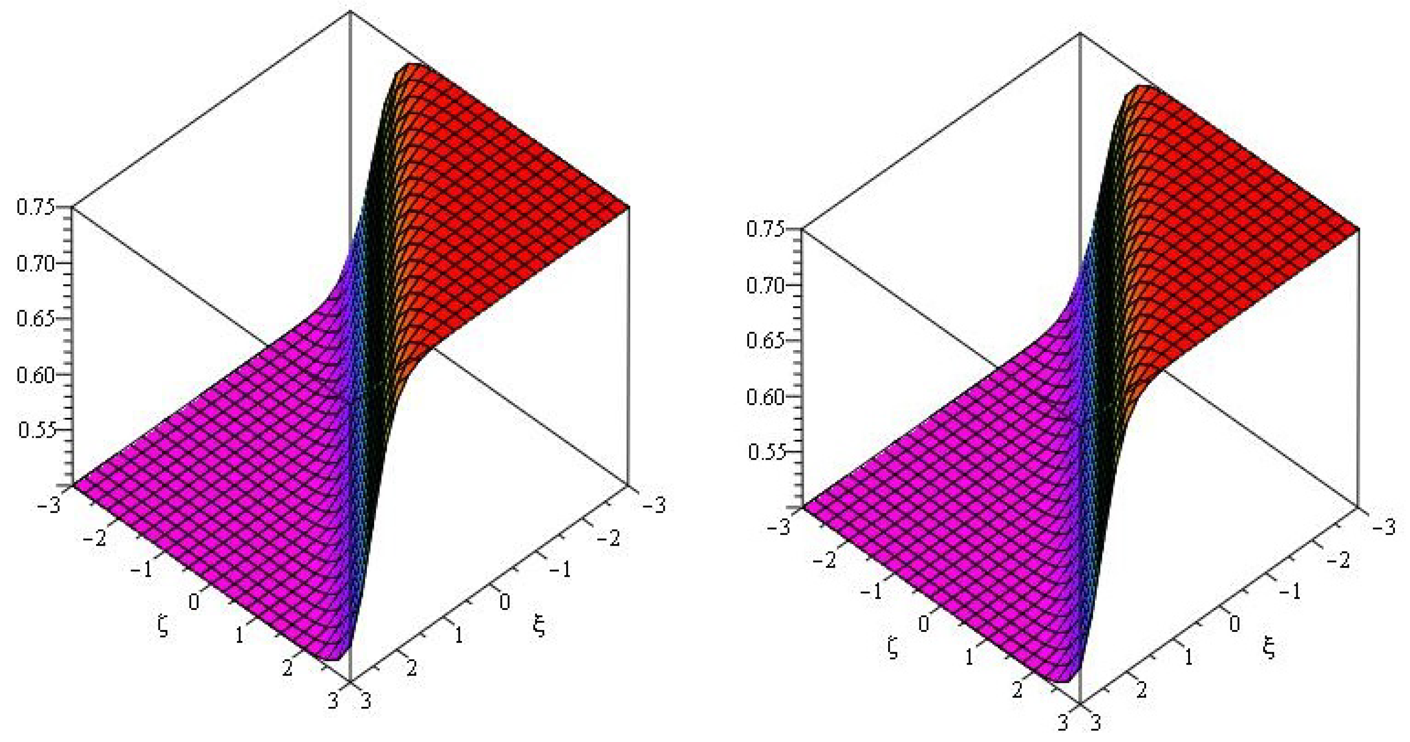
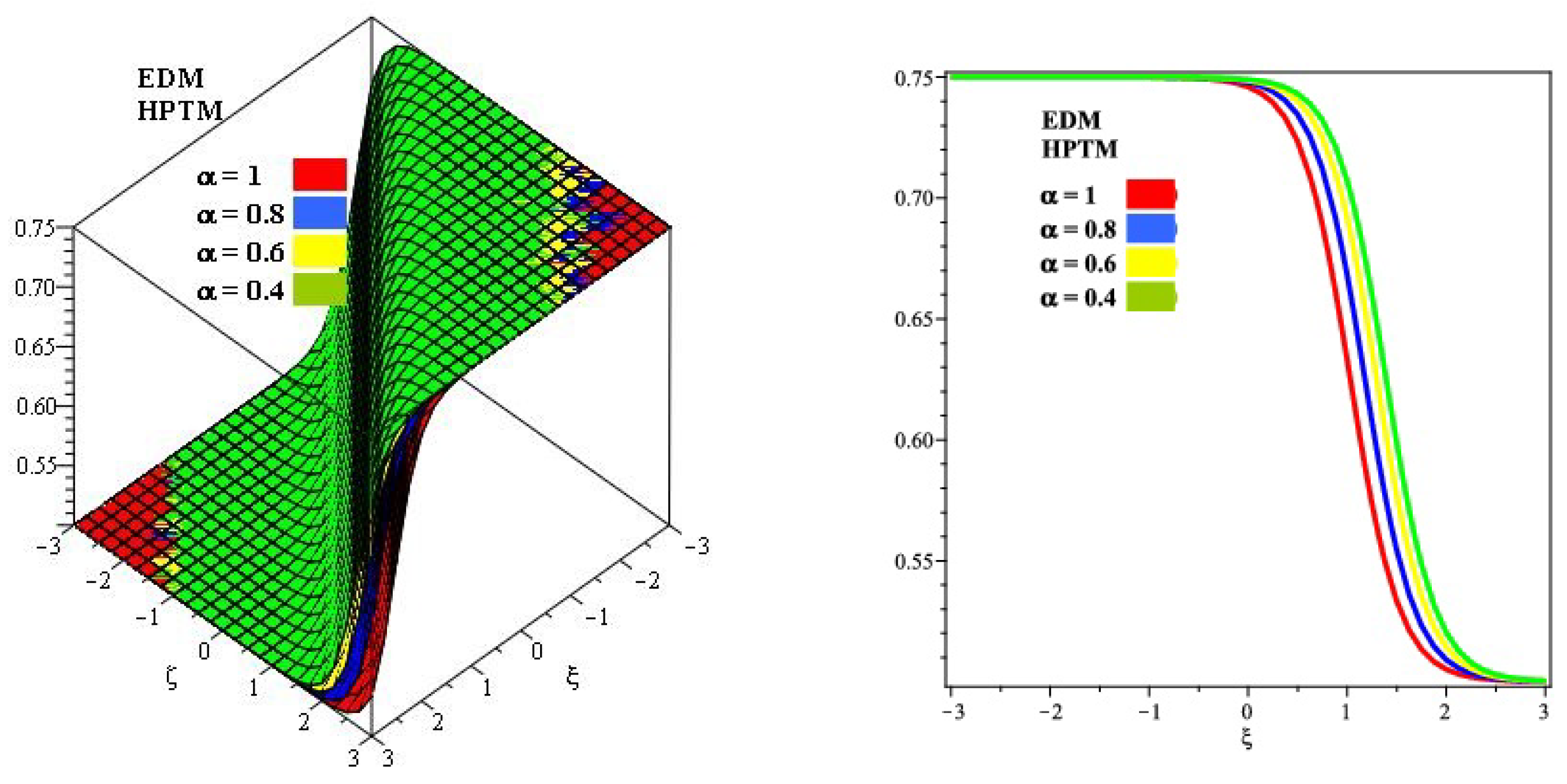
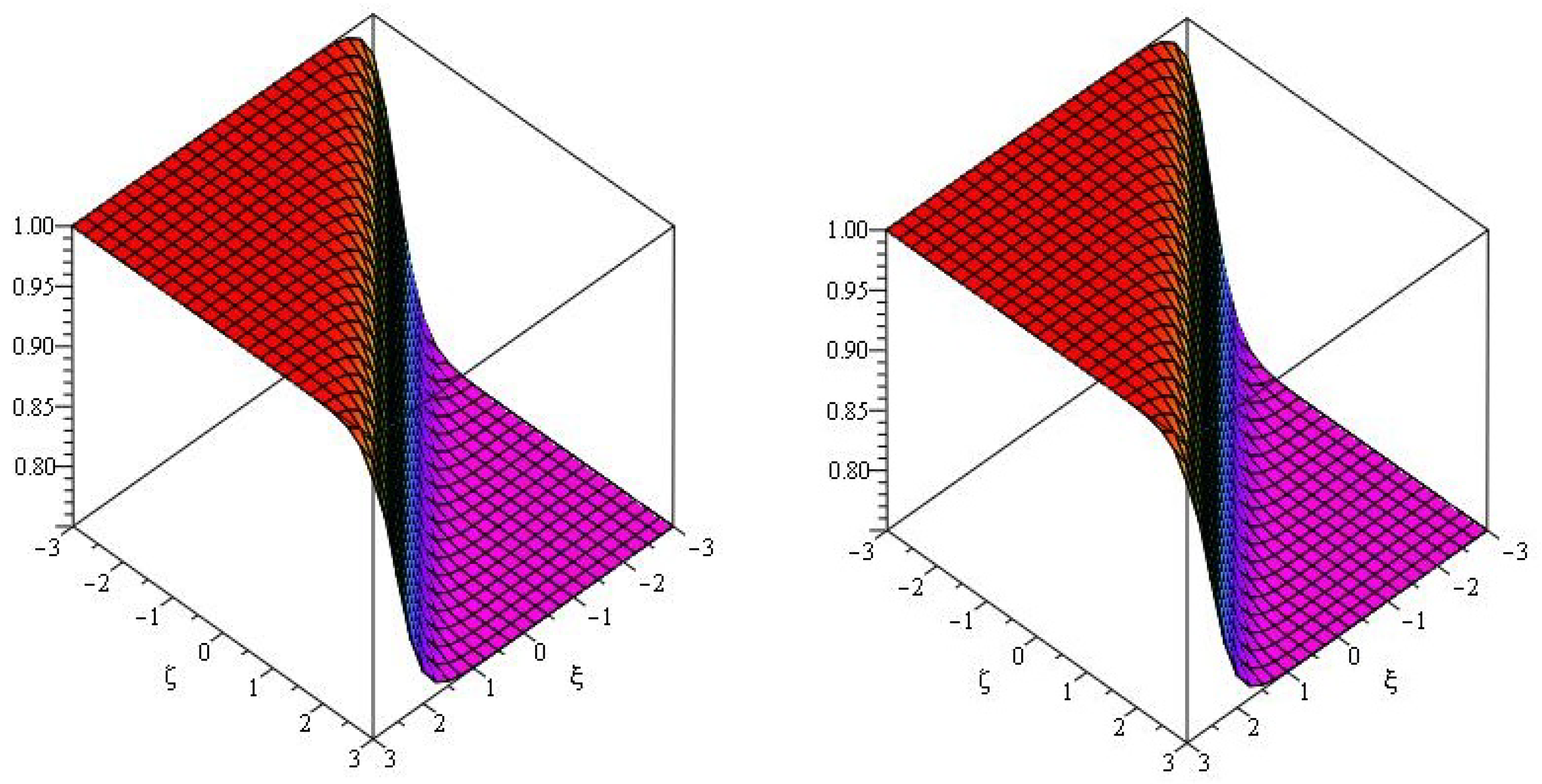
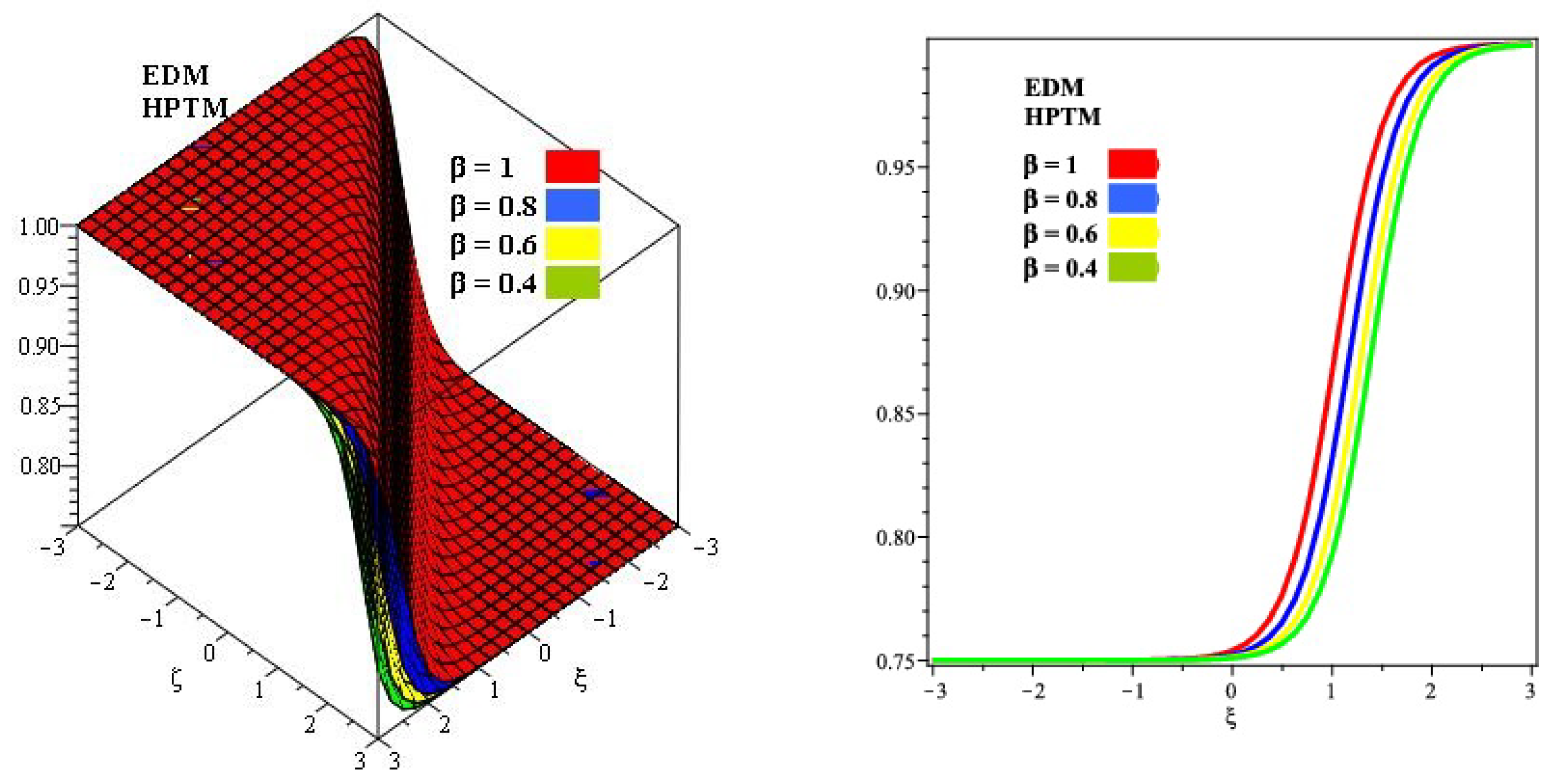
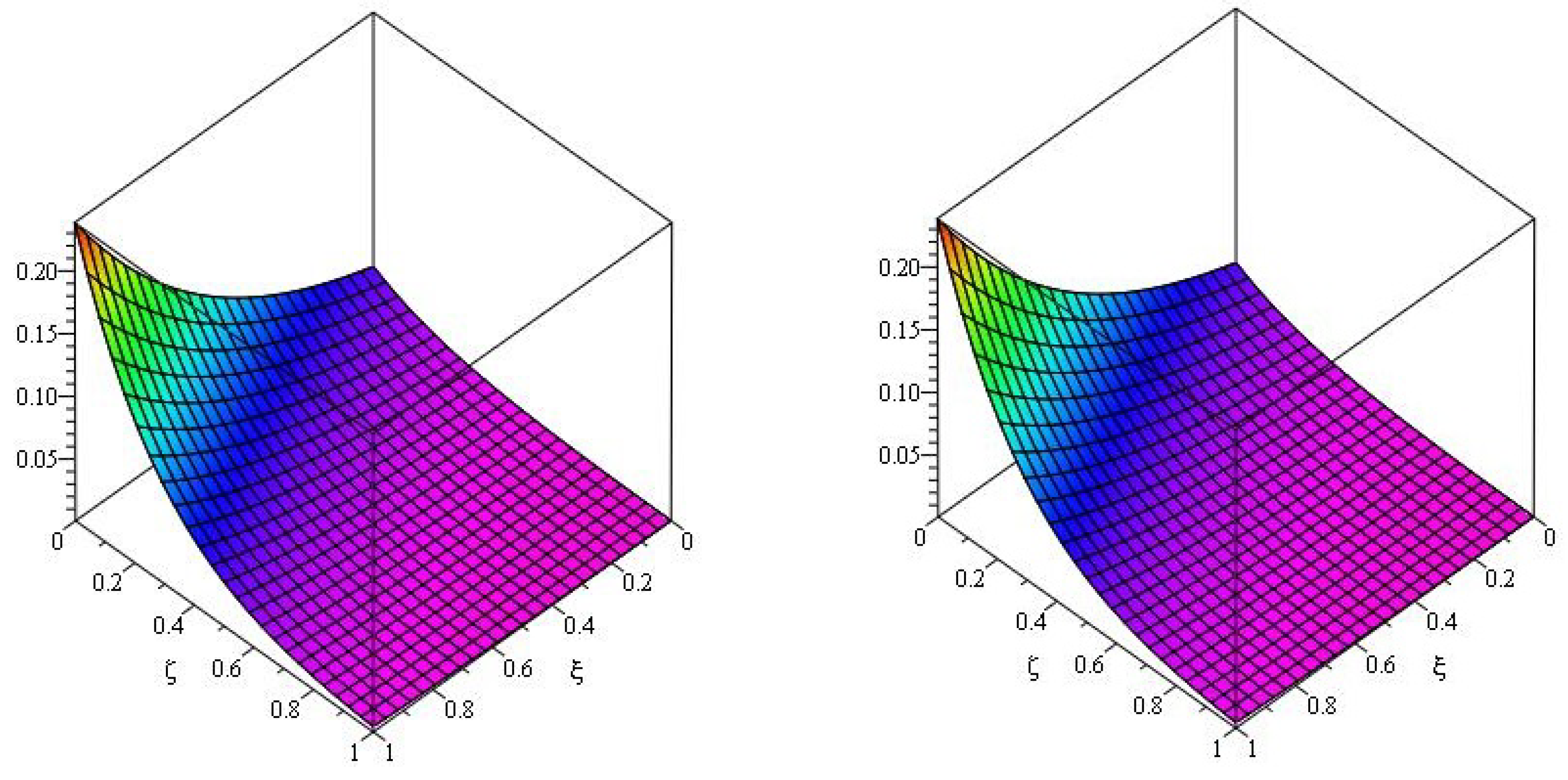
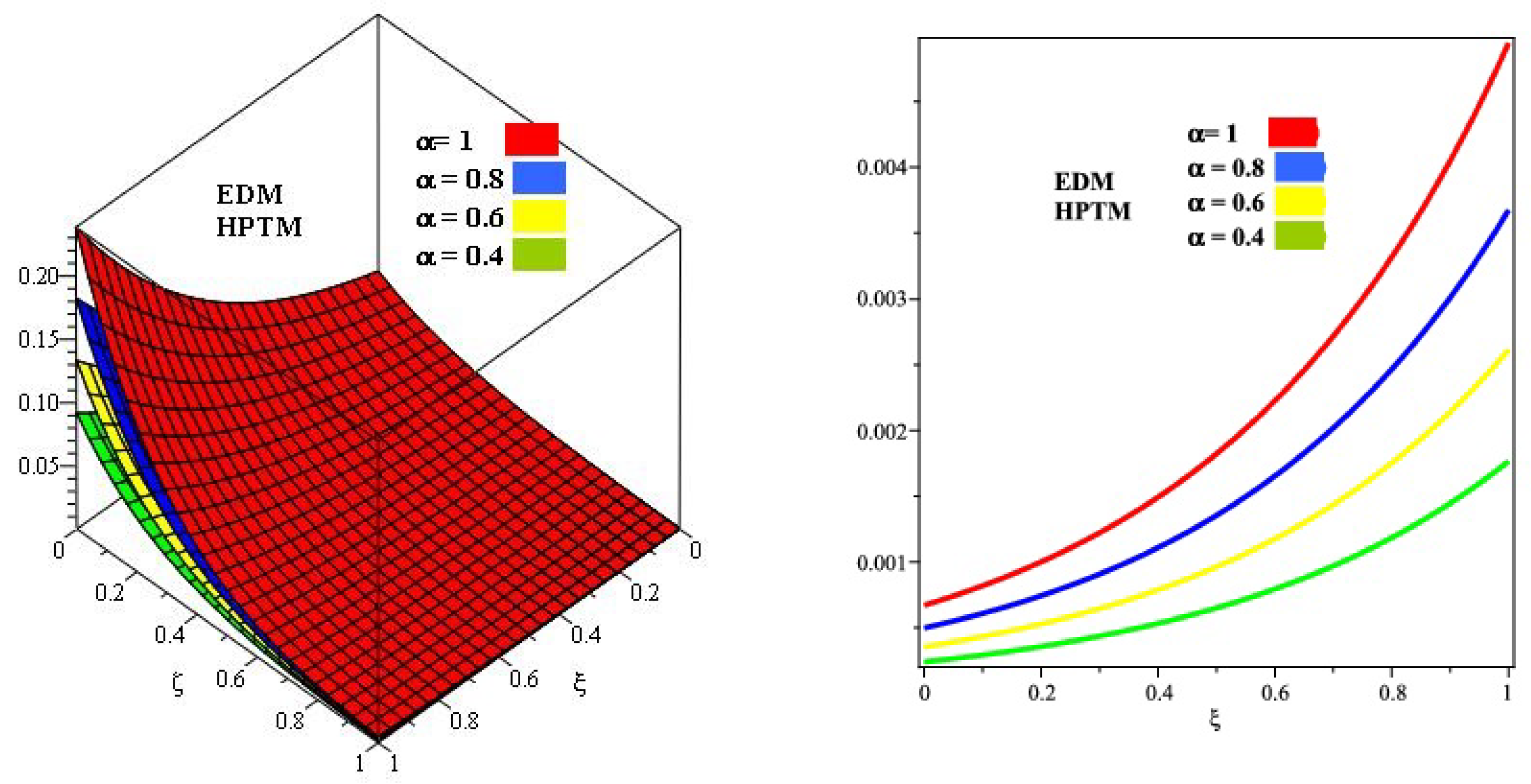
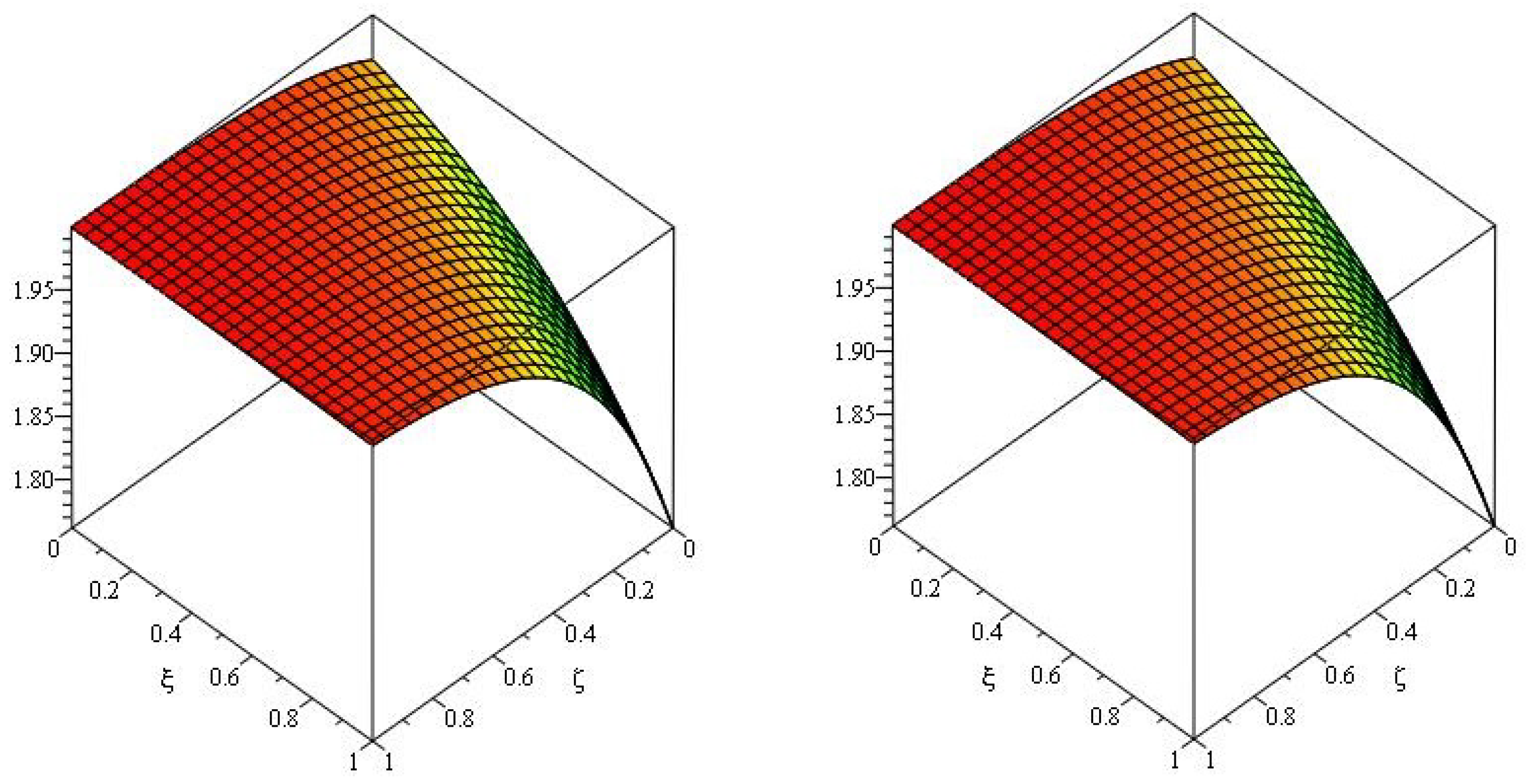
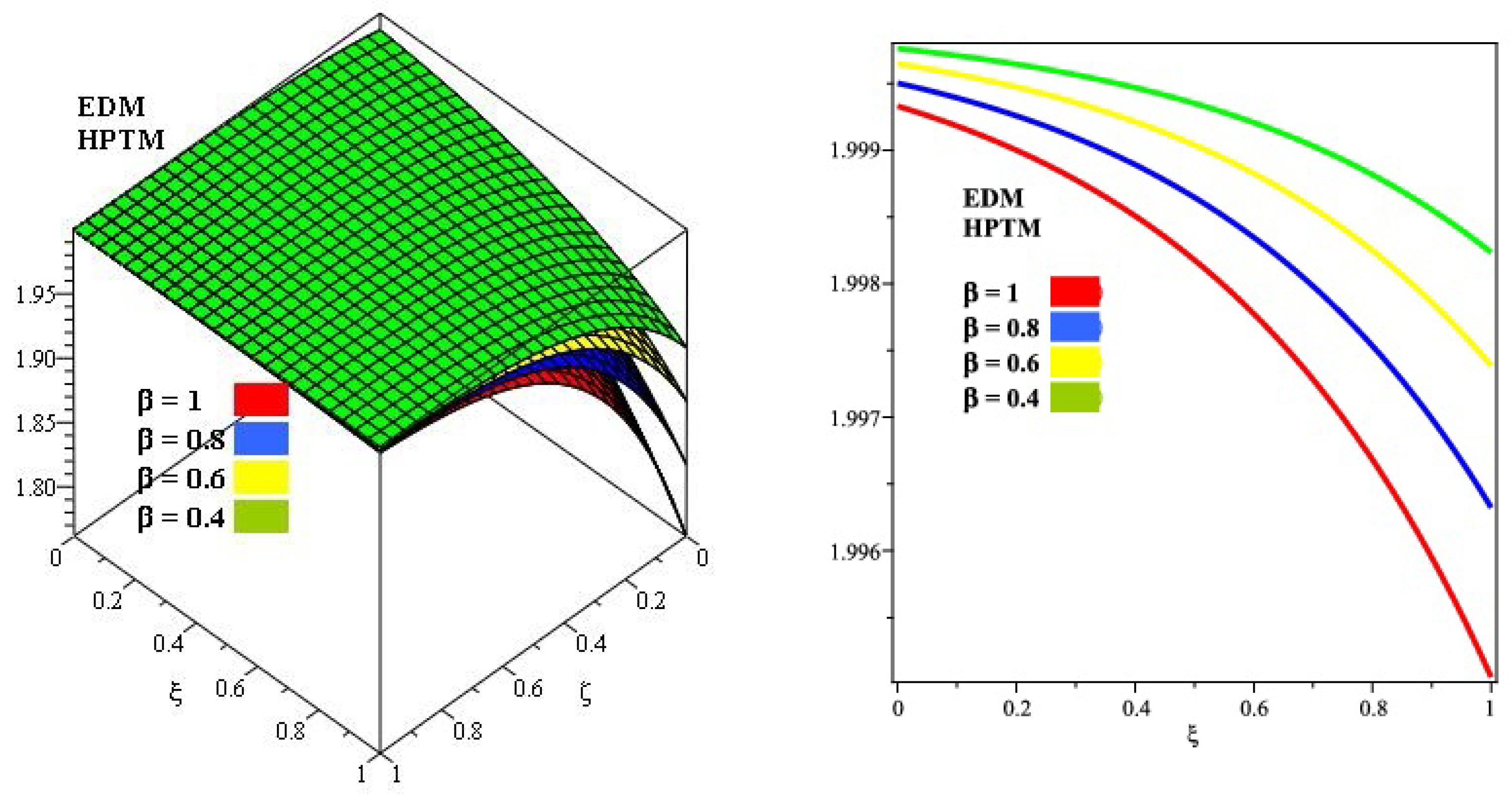
In Figure 1, show that the Elzaki decomposition method and Homotopy perturbation transform method show that the close contact with each other of Example 1. In Figure 2, represent the different fractional-order behaviour of $u(\xi ,\zeta ,\Im )$. Similarly, in Figure 3, show that the Elzaki decomposition method and Homotopy perturbation transform method show that the close contact with each other of Example 1. In Figure 4, represent the different fractional-order behaviour of $v(\xi ,\zeta ,\Im )$. In

Table 1. Numerical analysis of example 1 at $u(\xi ,\zeta ,\Im )$ different fractional-order of $\alpha$.

ℑ	$\mathit{\xi }$	AE ($\mathit{\alpha }=0.4$)	AE ($\mathit{\alpha }=0.6$)	AE ($\mathit{\alpha }=0.8)$	AE ($\mathit{\alpha }=1)$
	1	5.1298036$\times {10}^{-03}$	8.5968820$\times {10}^{-04}$	1.1526960$\times {10}^{-05}$	1.4693$\times {10}^{-10}$
	2	1.0533254900$\times {10}^{-02}$	1.7251291$\times {10}^{-03}$	2.3064850$\times {10}^{-05}$	2.1224$\times {10}^{-09}$
0.1	3	1.5936706200$\times {10}^{-02}$	2.5905700$\times {10}^{-03}$	3.4602750$\times {10}^{-05}$	2.7754$\times {10}^{-09}$
	4	2.1340157400$\times {10}^{-02}$	3.4560108$\times {10}^{-03}$	4.6140640$\times {10}^{-05}$	3.4285$\times {10}^{-09}$
	5	2.6743608600$\times {10}^{-02}$	4.3214516$\times {10}^{-03}$	5.7678540$\times {10}^{-05}$	4.0815$\times {10}^{-09}$
	1	6.5526269$\times {10}^{-03}$	1.2845443$\times {10}^{-04}$	1.9524030$\times {10}^{-05}$	8.9043500$\times {10}^{-08}$
	2	1.3585147$\times {10}^{-02}$	2.5823037$\times {10}^{-03}$	3.9081030$\times {10}^{-05}$	1.2243480$\times {10}^{-08}$
0.2	3	2.0617667100$\times {10}^{-03}$	3.8800631$\times {10}^{-03}$	5.8638020$\times {10}^{-05}$	1.5582620$\times {10}^{-08}$
	4	2.7650187200$\times {10}^{-02}$	5.1778225$\times {10}^{-03}$	7.8195020$\times {10}^{-05}$	1.8921750$\times {10}^{-08}$
	5	3.4682707200$\times {10}^{-02}$	6.4755819$\times {10}^{-03}$	9.7752020$\times {10}^{-05}$	2.2260880$\times {10}^{-08}$
	1	7.5239217$\times {10}^{-03}$	1.6203247$\times {10}^{-04}$	2.6503270$\times {10}^{-05}$	9.9570730$\times {10}^{-08}$
	2	1.5715901300$\times {10}^{-02}$	3.2621458$\times {10}^{-03}$	5.3069340$\times {10}^{-05}$	1.2801951$\times {10}^{-08}$
0.3	3	2.3907880800$\times {10}^{-02}$	4.9039669$\times {10}^{-03}$	7.9635420$\times {10}^{-05}$	1.5646829$\times {10}^{-08}$
	4	3.2099860300$\times {10}^{-02}$	6.5457880$\times {10}^{-03}$	1.0620149$\times {10}^{-05}$	1.8491707$\times {10}^{-08}$
	5	4.0291839800$\times {10}^{-02}$	8.1876092$\times {10}^{-03}$	1.3276756$\times {10}^{-05}$	2.1336585$\times {10}^{-08}$
	1	8.2762123$\times {10}^{-03}$	1.9075950$\times {10}^{-03}$	3.2874570$\times {10}^{-05}$	5.7825882$\times {10}^{-09}$
	2	1.7398405800$\times {10}^{-02}$	3.8455493$\times {10}^{-03}$	6.5848290$\times {10}^{-05}$	6.7463529$\times {10}^{-08}$
0.4	3	2.6520599300$\times {10}^{-02}$	5.7835036$\times {10}^{-03}$	9.8822010$\times {10}^{-05}$	7.7101176$\times {10}^{-08}$
	4	3.5642792800$\times {10}^{-02}$	7.7214580$\times {10}^{-03}$	1.3179574$\times {10}^{-05}$	8.6738823$\times {10}^{-08}$
	5	4.4764986200$\times {10}^{-02}$	9.6594122$\times {10}^{-03}$	1.6476946$\times {10}^{-05}$	9.6376470$\times {10}^{-08}$
	1	8.8947364$\times {10}^{-03}$	2.1627817$\times {10}^{-03}$	3.8817930$\times {10}^{-04}$	2.3900$\times {10}^{-08}$
	2	1.8806520800$\times {10}^{-02}$	4.3652454$\times {10}^{-03}$	7.7777130$\times {10}^{-04}$	3.5300$\times {10}^{-08}$
0.5	3	2.8718305200$\times {10}^{-02}$	6.5677091$\times {10}^{-03}$	1.1673633$\times {10}^{-05}$	4.6600$\times {10}^{-08}$
	4	3.8630089800$\times {10}^{-02}$	8.7701729$\times {10}^{-03}$	1.5569554$\times {10}^{-04}$	5.8$\times {10}^{-08}$
	5	4.8541874400$\times {10}^{-02}$	1.0972636700$\times {10}^{-03}$	1.9465475$\times {10}^{-04}$	6.9300000$\times {10}^{-08}$

and

Table 2. Numerical analysis of example 1 at $v(\xi ,\zeta ,\Im )$ at different fractional-order of $\alpha$.

ℑ	$\mathit{\xi }$	AE ($\mathit{\alpha }=0.4$)	AE ($\mathit{\alpha }=0.6$)	AE ($\mathit{\alpha }=0.8)$	AE ($\mathit{\alpha }=1)$
	1	5.6770988$\times {10}^{-04}$	8.7119340$\times {10}^{-05}$	1.1548840$\times {10}^{-07}$	1.6326$\times {10}^{-10}$
	2	5.3834512$\times {10}^{-03}$	8.4544080$\times {10}^{-04}$	9.5379000$\times {10}^{-07}$	2.0407510200$\times {10}^{-09}$
0.1	3	5.0898036$\times {10}^{-03}$	8.1968820$\times {10}^{-04}$	7.5269600$\times {10}^{-07}$	4.0814857200$\times {10}^{-09}$
	4	4.7961560$\times {10}^{-03}$	7.9393560$\times {10}^{-04}$	5.5160200$\times {10}^{-07}$	6.1222204100$\times {10}^{-09}$
	5	4.5025084$\times {10}^{-03}$	7.6818300$\times {10}^{-04}$	3.5050800$\times {10}^{-07}$	8.1629551100$\times {10}^{-09}$
	1	7.5124132$\times {10}^{-04}$	1.3109744$\times {10}^{-05}$	1.9589970$\times {10}^{-07}$	2.2260880$\times {10}^{-08}$
	2	6.9925200$\times {10}^{-03}$	1.2577593$\times {10}^{-04}$	1.5557000$\times {10}^{-07}$	4.3444869600$\times {10}^{-08}$
0.2	3	6.4726268$\times {10}^{-03}$	1.2045442$\times {10}^{-04}$	1.1524030$\times {10}^{-07}$	8.6867478200$\times {10}^{-08}$
	4	5.9527336$\times {10}^{-03}$	1.1513291$\times {10}^{-04}$	7.4910600$\times {10}^{-06}$	1.3029008690$\times {10}^{-08}$
	5	5.4328404$\times {10}^{-03}$	1.0981140$\times {10}^{-04}$	3.4580900$\times {10}^{-06}$	1.7371269560$\times {10}^{-08}$
	1	8.8600372900$\times {10}^{-04}$	1.6633175900$\times {10}^{-05}$	2.6628869$\times {10}^{-06}$	4.2673170$\times {10}^{-08}$
	2	8.1319795$\times {10}^{-03}$	1.5818212$\times {10}^{-04}$	2.0566070$\times {10}^{-06}$	7.2886243900$\times {10}^{-08}$
0.3	3	7.4039217$\times {10}^{-03}$	1.5003248$\times {10}^{-04}$	1.4503270$\times {10}^{-06}$	1.4534575610$\times {10}^{-08}$
	4	6.6758639$\times {10}^{-03}$	1.4188284$\times {10}^{-04}$	8.4404700$\times {10}^{-06}$	2.1780526830$\times {10}^{-08}$
	5	5.9478061$\times {10}^{-03}$	1.3373320$\times {10}^{-04}$	2.3776700$\times {10}^{-06}$	2.9026478050$\times {10}^{-08}$
	1	9.9681746700$\times {10}^{-04}$	1.9683136700$\times {10}^{-04}$	3.3072887$\times {10}^{-06}$	3.8550588$\times {10}^{-09}$
	2	9.0421934$\times {10}^{-03}$	1.8579543$\times {10}^{-04}$	2.4973720$\times {10}^{-06}$	1.1668329410$\times {10}^{-08}$
0.4	3	8.1162122$\times {10}^{-03}$	1.7475950$\times {10}^{-04}$	1.6874560$\times {10}^{-06}$	2.2951152940$\times {10}^{-08}$
	4	7.1902310$\times {10}^{-03}$	1.6372357$\times {10}^{-04}$	8.7754000$\times {10}^{-06}$	3.4233976470$\times {10}^{-08}$
	5	6.2642497$\times {10}^{-03}$	1.5268763$\times {10}^{-04}$	6.7623000$\times {10}^{-06}$	4.5516800$\times {10}^{-08}$
	1	1.0928832650$\times {10}^{-04}$	2.2421458500$\times {10}^{-04}$	3.9100485$\times {10}^{-06}$	1.2600000$\times {10}^{-08}$
	2	9.8117844$\times {10}^{-03}$	2.1024637$\times {10}^{-04}$	2.8959200$\times {10}^{-06}$	1.0050239900$\times {10}^{-08}$
0.5	3	8.6947361$\times {10}^{-03}$	1.9627815$\times {10}^{-04}$	1.8817910$\times {10}^{-06}$	2.0100478600$\times {10}^{-08}$
	4	7.5776879$\times {10}^{-03}$	1.8230994$\times {10}^{-04}$	8.6766300$\times {10}^{-06}$	3.0150717200$\times {10}^{-08}$
	5	6.4606397$\times {10}^{-03}$	1.6834173$\times {10}^{-04}$	1.4646500$\times {10}^{-06}$	4.0200955900$\times {10}^{-08}$

show that the absolute error with different fractional-order with respect to $\alpha$ and $\beta$.

Example 2.

Consider the fractional-order system of Burgers equations

$$\begin{array}{cc}\hfill D_{\Im }^{\alpha }u& =2u\frac{\partial u}{\partial \xi }+2v\frac{\partial u}{\partial \zeta }+\frac{{\partial }^{2}u}{\partial {\xi }^2}+\frac{{\partial }^{2}u}{\partial {\zeta }^2},\hfill \\ \hfill D_{\Im }^{\beta }v& =2u\frac{\partial v}{\partial \xi }+2v\frac{\partial v}{\partial \zeta }+\frac{{\partial }^{2}v}{\partial {\xi }^2}+\frac{{\partial }^{2}v}{\partial {\zeta }^2},0<\alpha ,\beta \le 1,\hfill \end{array}$$

(37)

with initial conditions

$$\begin{array}{cc}\hfill u(\xi ,\zeta ,0)& =1-tanh(-\xi +2\zeta +1),\hfill \\ \hfill v(\xi ,\zeta ,0)& =1-2tanh(-\xi +2\zeta +1).\hfill \end{array}$$

(38)

Now by using $ET$ on Equation (37), we get series solutions

$$\begin{array}{cc}\hfill E\left[D_{\Im }^{\alpha }u(\xi ,\zeta ,\Im )\right]& =E\left[2u\frac{\partial u}{\partial \xi }\right]+E\left[2v\frac{\partial u}{\partial \zeta }\right]+E\left[\frac{{\partial }^{2}u}{\partial {\xi }^2}\right]+E\left[\frac{{\partial }^{2}u}{\partial {\zeta }^2}\right],\hfill \\ \hfill E\left[D_{\Im }^{\beta }v(\xi ,\zeta ,\Im )\right]& =E\left[2u\frac{\partial v}{\partial \xi }\right]+E\left[2v\frac{\partial v}{\partial \zeta }\right]+E\left[\frac{{\partial }^{2}v}{\partial {\xi }^2}\right]+E\left[\frac{{\partial }^{2}v}{\partial {\zeta }^2}\right].\hfill \end{array}$$

(39)

Define the non-linear operator as

$$\begin{array}{cc}\hfill \frac{1}{s^{\alpha }}E\left[u(\xi ,\zeta ,\Im )\right]-s^{2-\alpha }u(\xi ,\zeta ,0)& =E\left[2u\frac{\partial u}{\partial \xi }+2v\frac{\partial u}{\partial \zeta }+\frac{{\partial }^{2}u}{\partial {\xi }^2}+\frac{{\partial }^{2}u}{\partial {\zeta }^2}\right],\hfill \\ \hfill \frac{1}{s^{\beta }}E\left[v(\xi ,\zeta ,\Im )\right]-s^{2-\beta }u(\xi ,\zeta ,0)& =E\left[2u\frac{\partial v}{\partial \xi }+2v\frac{\partial v}{\partial \zeta }+\frac{{\partial }^{2}u}{\partial {\xi }^2}+\frac{{\partial }^{2}u}{\partial {\zeta }^2}\right].\hfill \end{array}$$

(40)

On simplification, the above equation reduces to

$$\begin{array}{cc}\hfill E\left[u\right(\xi ,\zeta ,\Im \left)\right]& =s^2\left[1-tanh(-\xi +2\zeta +1)\right]+s^{\alpha }\left[2u\frac{\partial u}{\partial \xi }+2v\frac{\partial u}{\partial \zeta }+\frac{{\partial }^{2}u}{\partial {\xi }^2}+\frac{{\partial }^{2}u}{\partial {\zeta }^2}\right],\hfill \\ \hfill E\left[v\right(\xi ,\zeta ,\Im \left)\right]& =s^2\left[1+2tanh(-\xi +2\zeta +1)\right]+s^{\beta }\left[2u\frac{\partial v}{\partial \xi }+2v\frac{\partial v}{\partial \zeta }+\frac{{\partial }^{2}v}{\partial {\xi }^2}+\frac{{\partial }^{2}v}{\partial {\zeta }^2}\right].\hfill \end{array}$$

(41)

Applying inverse $ET$ on Equation (41), we have

$$\begin{array}{cc}\hfill u(\xi ,\zeta ,\Im )& =1-tanh(-\xi +2\zeta +1)+E^{-1}\left[s^{\alpha }\left\{2u{u}_{\xi }+2v{u}_y+u_{\xi \xi }+u_{\zeta \zeta }\right\}\right],\hfill \\ \hfill v(\xi ,\zeta ,\Im )& =1+2tanh(-\xi +2\zeta +1)+E^{-1}\left[s^{\beta }\left\{2u{v}_{\xi }+2v{v}_y+v_{\xi \xi }+v_{\zeta \zeta }\right\}\right].\hfill \end{array}$$

(42)

Now we implement HPM

$$\begin{array}{cc}\hfill \sum _{\omega =0}^{\infty }{p}^{\omega }{u}_{\omega }(\xi ,\zeta ,\Im )=& 1-tanh(-\xi +2\zeta +1)\hfill \\ \hfill & +p\left[E^{-1}\left\{s^{\alpha }E\left(\left(\sum _{\omega =0}^{\infty }{p}^{\omega }\left(\frac{{\partial }^2{u}_{\omega }}{\partial {\xi }^2}+\frac{{\partial }^2{u}_{\omega }}{\partial {\zeta }^2}\right)\right)+\left(\sum _{\omega =0}^{\infty }{p}^{\omega }{H}_{\omega }\left(u\right)\right)\right)\right\}\right].\hfill \\ \hfill \sum _{\omega =0}^{\infty }{p}^{\omega }{v}_{\omega }(\xi ,\zeta ,\Im )=& 1+2tanh(-\xi +2\zeta +1)\hfill \\ \hfill & +p\left[E^{-1}\left\{s^{\beta }E\left(\left(\sum _{\omega =0}^{\infty }{p}^{\omega }\left(\frac{{\partial }^2{v}_{\omega }}{\partial {\xi }^2}+\frac{{\partial }^2{v}_{\omega }}{\partial {\zeta }^2}\right)\right)+\left(\sum _{\omega =0}^{\infty }{p}^{\omega }{H}_{\omega }\left(v\right)\right)\right)\right\}\right].\hfill \end{array}$$

(43)

With the aid of He’s polynomials $H_{\omega }\left(u\right)$ and $H_{\omega }\left(v\right)$, the nonlinear terms can be found

$${\mathrm{\Sigma }}_{\omega =0}^{\infty }{p}^{\omega }{H}_{\omega }\left(u\right)=2u{u}_{\xi }+2v{u}_{\zeta },{\mathrm{\Sigma }}_{\omega =0}^{\infty }{p}^{\omega }{H}_{\omega }\left(v\right)=2u{v}_{\xi }+2v{v}_{\zeta }.$$

(44)

He’s polynomials are expressed as

$$\begin{array}{cc}\hfill H_0\left(u\right)& =2u_0{u_0}_{\xi }+2v_0{u_0}_{\zeta },H_0\left(v\right)=2u_0{v_0}_{\xi }+2v_0{v_0}_{\zeta },\hfill \\ \hfill H_1\left(u\right)& =2u_0{u_1}_{\xi }+2u_1{u_0}_{\xi }+2v_0{u_1}_{\zeta }+2v_1{u_0}_{\zeta },H_1\left(v\right)=2u_0{v_1}_{\xi }+2u_1{v_0}_{\xi }+2v_0{v_1}_{\zeta }+2v_1{v_0}_{\zeta },\hfill \\ \hfill ⋮\end{array}$$

Comparing p-like coefficients, we get

$$\begin{array}{cc}\hfill p^0:u_0(\xi ,\zeta ,\Im )=& 1-tanh(-\xi +2\zeta +1),\hfill \\ \hfill p^0:v_0(\xi ,\zeta ,\Im )=& 1+2tanh(-\xi +2\zeta +1),\hfill \\ \hfill p^1:u_1(\xi ,\zeta ,\Im )=& E^{-1}\left\{s^{\alpha }E\left(\left(\frac{{\partial }^2{u}_0}{\partial {\xi }^2}+\frac{{\partial }^2{u}_0}{\partial {\zeta }^2}\right)+H_0\left(u\right)\right)\right\}.\hfill \\ \hfill p^1:v_1(\xi ,\zeta ,\Im )=& E^{-1}\left\{s^{\beta }E\left(\left(\frac{{\partial }^2{v}_0}{\partial {\xi }^2}+\frac{{\partial }^2{v}_0}{\partial {\zeta }^2}\right)+H_0\left(v\right)\right)\right\}.\hfill \\ \hfill p^1:u_1(\xi ,\zeta ,\Im )& =-\frac{2sech(-\xi +2\zeta +1){\Im }^{\alpha }}{\mathrm{\Gamma }(\alpha +1)},\hfill \\ \hfill p^1:v_1(\xi ,\zeta ,\Im )& =\frac{4sech(-\xi +2\zeta +1){\Im }^{\beta }}{\mathrm{\Gamma }(\beta +1)}.\hfill \end{array}$$

$$\begin{array}{cc}\hfill p^2:u_2(\xi ,\zeta ,\Im )& =E^{-1}\left\{s^{\alpha }E\left(\left(\frac{{\partial }^2{u}_1}{\partial {\xi }^2}+\frac{{\partial }^2{u}_1}{\partial {\zeta }^2}\right)+H_1\left(u\right)\right)\right\}.\hfill \\ \hfill p^2:v_2(\xi ,\zeta ,\Im )& =E^{-1}\left\{s^{\beta }E\left(\left(\frac{{\partial }^2{v}_1}{\partial {\xi }^2}+\frac{{\partial }^2{v}_1}{\partial {\zeta }^2}\right)+H_1\left(v\right)\right)\right\}.\hfill \\ \hfill u_2(\xi ,\zeta ,\Im )& =\frac{8sec{h}^2(-\xi +2\zeta +1)}{\mathrm{\Gamma }(\alpha +\beta +1)}(-2{\Im }^{\beta }\mathrm{\Gamma }(\alpha +1)sec{h}^2(-\xi +2\zeta +1)\hfill \\ \hfill & +{\Im }^{\beta }\mathrm{\Gamma }(\beta +1)(2sec{h}^2(-\xi +2\zeta +1)+tanh(-\xi +2\zeta +1))),\hfill \\ \hfill v_2(\xi ,\zeta ,\Im )& =-\frac{8sec{h}^2(-\xi +2\zeta +1)}{\mathrm{\Gamma }(\alpha +\beta +1)}(-{\Im }^{\beta }\mathrm{\Gamma }(\alpha +1)sec{h}^2(-\xi +2\zeta +1)\hfill \\ \hfill & +{\Im }^{\beta }\mathrm{\Gamma }(\beta +1)(2sec{h}^2(-\xi +2\zeta +1)+2tanh(-\xi +2\zeta +1))).\hfill \\ \hfill & ⋮\end{array}$$

Provides the series form result is $u(\xi ,\zeta ,\Im )={\mathrm{\Sigma }}_{\omega =0}^{\infty }{u}_{\omega }(\xi ,\zeta ,\Im )$ and $v(\xi ,\zeta ,\Im )={\mathrm{\Sigma }}_{\omega =0}^{\infty }{v}_{\omega }$$(\xi ,\zeta ,\Im )$

$$\begin{array}{cc}\hfill u(\xi ,\zeta ,\Im )& =1-tanh(-\xi +2\zeta +1)-\frac{2sech(-\xi +2\zeta +1){\Im }^{\alpha }}{\mathrm{\Gamma }(\alpha +1)}\hfill \\ \hfill & +\frac{8sec{h}^2(-\xi +2\zeta +1)}{\mathrm{\Gamma }(\alpha +\beta +1)}(-2{\Im }^{\beta }\mathrm{\Gamma }(\alpha +1)sec{h}^2(-\xi +2\zeta +1)\hfill \\ \hfill & +{\Im }^{\beta }\mathrm{\Gamma }(\beta +1)(2sec{h}^2(-\xi +2\zeta +1)+tanh(-\xi +2\zeta +1)))+\cdots ,\hfill \\ \hfill v(\xi ,\zeta ,\Im )& =1+2tanh(-\xi +2\zeta +1)+\frac{4sech(-\xi +2\zeta +1){\Im }^{\beta }}{\mathrm{\Gamma }(\beta +1)}\hfill \\ \hfill & -\frac{8sec{h}^2(-\xi +2\zeta +1)}{\mathrm{\Gamma }(\alpha +\beta +1)}(-{\Im }^{\beta }\mathrm{\Gamma }(\alpha +1)sec{h}^2(-\xi +2\zeta +1)\hfill \\ \hfill & +{\Im }^{\beta }\mathrm{\Gamma }(\beta +1)(2sec{h}^2(-\xi +2\zeta +1)+2tanh(-\xi +2\zeta +1)))+\cdots .\hfill \end{array}$$

(45)

Now we apply EDM

Suppose that the unidentified functions have an infinite series result $u(\xi ,\zeta ,\Im )$ and $v(\xi ,\zeta ,\Im )$ respectively as follows

$$\begin{array}{c}\hfill u(\xi ,\zeta ,\Im )=\sum _{\omega =0}^{\infty }{u}_{\omega }(\xi ,\zeta ,\Im )andv(\xi ,\zeta ,\Im )=\sum _{\omega =0}^{\infty }{v}_{\omega }(\xi ,\zeta ,\Im )\end{array}$$

(46)

Note that $u{u}_{\xi }={\sum }_{\omega =0}^{\infty }{A}_{\omega }$, $u{v}_{\xi }={\sum }_{\omega =0}^{\infty }{B}_{\omega }$, $v{u}_{\xi }={\sum }_{\omega =0}^{\infty }{C}_{\omega }$ and $v{v}_{\xi }={\sum }_{\omega =0}^{\infty }{D}_{\omega }$ are the Adomian polynomials and they signifying the non-linear terms. Applying the these terms, we can be write Equation (42) as

$$\begin{array}{cc}\hfill \sum _{n=0}^{\infty }{u}_{\omega }(\xi ,\zeta ,\Im )& =\left[1-tanh(-\xi +2\zeta +1)\right]+E^{-1}\left[s^{\alpha }\left[2\sum _{\omega =0}^{\infty }{A}_{\omega }+2\sum _{\omega =0}^{\infty }{B}_{\omega }+\sum _{\omega =0}^{\infty }{u}_{\omega \xi \xi }+\sum _{\omega =0}^{\infty }{u}_{\omega \zeta \zeta }\right]\right],\hfill \\ \hfill \sum _{n=0}^{\infty }{v}_{\omega }(\xi ,\zeta ,\Im )& =\left[1+2tanh(-\xi +2\zeta +1)\right]+E^{-1}\left[s^{\beta }\left[2\sum _{\omega =0}^{\infty }{C}_{\omega }+2\sum _{\omega =0}^{\infty }{D}_{\omega }+\sum _{\omega =0}^{\infty }{v}_{\omega \xi \xi }+\sum _{\omega =0}^{\infty }{v}_{\omega \zeta \zeta }\right]\right].\hfill \end{array}$$

(47)

Comparing both sides of Equation (47), they can be written as follows

$$\begin{array}{cc}\hfill u_0(\xi ,\zeta ,\Im )& =1-tanh(-\xi +2\zeta +1),\hfill \\ \hfill v_0(\xi ,\zeta ,\Im )& =1+2tanh(-\xi +2\zeta +1).\hfill \\ \hfill u_1(\xi ,\zeta ,\Im )& =-\frac{2sech(-\xi +2\zeta +1){\Im }^{\alpha }}{\mathrm{\Gamma }(\alpha +1)},\hfill \\ \hfill v_1(\xi ,\zeta ,\Im )& =\frac{4sech(-\xi +2\zeta +1){\Im }^{\beta }}{\mathrm{\Gamma }(\beta +1)}.\hfill \\ \hfill u_2(\xi ,\zeta ,\Im )& =\frac{8sec{h}^2(-\xi +2\zeta +1)}{\mathrm{\Gamma }(\alpha +\beta +1)}(-2{\Im }^{\beta }\mathrm{\Gamma }(\alpha +1)sec{h}^2(-\xi +2\zeta +1)\hfill \\ \hfill & +{\Im }^{\beta }\mathrm{\Gamma }(\beta +1)(2sec{h}^2(-\xi +2\zeta +1)+tanh(-\xi +2\zeta +1))),\hfill \\ \hfill v_2(\xi ,\zeta ,\Im )& =-\frac{8sec{h}^2(-\xi +2\zeta +1)}{\mathrm{\Gamma }(\alpha +\beta +1)}(-{\Im }^{\beta }\mathrm{\Gamma }(\alpha +1)sec{h}^2(-\xi +2\zeta +1)\hfill \\ \hfill & +{\Im }^{\beta }\mathrm{\Gamma }(\beta +1)(2sec{h}^2(-\xi +2\zeta +1)+2tanh(-\xi +2\zeta +1))).\hfill \end{array}$$

(48)

Proceeding in the same manner, the remaining components of the Elzaki decomposition method (EDM) solution $u_{\omega }$ and $v_{\omega }(\omega \ge 3)$ can be achieved smoothly. As a result, we arrive at the series solution as

$$\begin{array}{cc}\hfill u(\xi ,\zeta ,\Im )& =\sum _{\omega =0}^{\infty }{u}_{\omega }(\xi ,\zeta ,\Im )=u_0(\xi ,\zeta ,\Im )+u_1(\xi ,\zeta ,\Im )+u_2(\xi ,\zeta ,\Im )+\cdots ,\hfill \\ \hfill u(\xi ,\zeta ,\Im )& =1-tanh(-\xi +2\zeta +1)-\frac{2sech(-\xi +2\zeta +1){\Im }^{\alpha }}{\mathrm{\Gamma }(\alpha +1)}\hfill \\ \hfill & +\frac{8sec{h}^2(-\xi +2\zeta +1)}{\mathrm{\Gamma }(\alpha +\beta +1)}(-2{\Im }^{\beta }\mathrm{\Gamma }(\alpha +1)sec{h}^2(-\xi +2\zeta +1)\hfill \\ \hfill & +{\Im }^{\beta }\mathrm{\Gamma }(\beta +1)(2sec{h}^2(-\xi +2\zeta +1)+tanh(-\xi +2\zeta +1)))+\cdots ,\hfill \\ \hfill v(\xi ,\zeta ,\Im )& =\sum _{\omega =0}^{\infty }{v}_{\omega }(\xi ,\zeta ,\Im )=v_0(\xi ,\zeta ,\Im )+v_1(\xi ,\zeta ,\Im )+v_2(\xi ,\zeta ,\Im )+\cdots ,\hfill \\ \hfill v(\xi ,\zeta ,\Im )& =1+2tanh(-\xi +2\zeta +1)+\frac{4sech(-\xi +2\zeta +1){\Im }^{\beta }}{\mathrm{\Gamma }(\beta +1)}\hfill \\ \hfill & -\frac{8sec{h}^2(-\xi +2\zeta +1)}{\mathrm{\Gamma }(\alpha +\beta +1)}(-{\Im }^{\beta }\mathrm{\Gamma }(\alpha +1)sec{h}^2(-\xi +2\zeta +1)\hfill \\ \hfill & +{\Im }^{\beta }\mathrm{\Gamma }(\beta +1)(2sec{h}^2(-\xi +2\zeta +1)+2tanh(-\xi +2\zeta +1)))+\cdots .\hfill \end{array}$$

(49)

The exact solution for Equation (37) is given by

$$\begin{array}{c}\hfill u(\xi ,\zeta ,\Im )=1-tanh(-\xi +2\zeta +2\Im +1),\\ \hfill v(\xi ,\zeta ,\Im )=1+2tanh(-\xi +2\zeta +2\Im +1).\end{array}$$

(50)

In Figure 5, show that the Elzaki decomposition method and Homotopy perturbation transform method show that the close contact with each other of Example 2. In Figure 6, represent the different fractional-order behaviour of $u(\xi ,\zeta ,\Im )$. Similarly, in Figure 7, show that the Elzaki decomposition method and Homotopy perturbation transform method show that the close contact with each other of Example 2. In Figure 8, represent the different fractional-order behaviour of $v(\xi ,\zeta ,\Im )$.

5. Conclusions

In the present article, the homotopy perturbation method and Elzaki decomposition method are applied for the solution of coupled systems of fractional Burger equations. The graphical and tabular representations of the derived results have been done. These representations of the obtained results have clearly confirmed the higher accuracy of the suggested methods. The solutions are obtained for fractional systems which are closely related to their actual solutions. The convergence of fractional solutions to integer order solution has been shown. The fewer calculations and higher accuracy are the valuable themes of the present methods. The researchers then modified it to solve other systems with fractional partial differential equations.

References

- Sabatier, J.A.T.M.J.; Agrawal, O.P.; Machado, J.T. Advances in Fractional Calculus; Springer: Dordrecht, The Netherlands, 2007; Volume 4, No. 9. [Google Scholar]
- Atangana, A.; Baleanu, D. Caputo-Fabrizio derivative applied to groundwater flow within confined aquifer. J. Eng. Mech. 2017, 143, D4016005. [Google Scholar] [CrossRef]
- Madani, M.; Fathizadeh, M.; Khan, Y.; Yildirim, A. On the coupling of the homotopy perturbation method and Laplace transformation. Math. Comput. Model. 2011, 53, 1937–1945. [Google Scholar] [CrossRef]
- Naeem, M.; Zidan, A.; Nonlaopon, K.; Syam, M.; Al-Zhour, Z.; Shah, R. A New Analysis of Fractional-Order Equal-Width Equations via Novel Techniques. Symmetry 2021, 13, 886. [Google Scholar] [CrossRef]
- Morales-Delgado, V.F.; Gómez-Aguilar, J.F.; Yépez-Martínez, H.; Baleanu, D.; Escobar-Jimenez, R.F.; Olivares-Peregrino, V.H. Laplace homotopy analysis method for solving linear partial differential equations using a fractional derivative with and without kernel singular. Adv. Differ. Equ. 2016, 2016, 164. [Google Scholar] [CrossRef] [Green Version]
- Li, Y.; Nohara, B.T.; Liao, S. Series solutions of coupled Van der Pol equation by means of homotopy analysis method. J. Math. Phys. 2010, 51, 063517. [Google Scholar] [CrossRef] [Green Version]
- Keskin, Y.; Oturanc, G. Reduced differential transform method for partial differential equations. Int. J. Nonlinear Sci. Numer. Simul. 2009, 10, 741–750. [Google Scholar] [CrossRef]
- Gupta, P.K. Approximate analytical solutions of fractional Benney—Lin equation by reduced differential transform method and the homotopy perturbation method. Comput. Math. Appl. 2011, 61, 2829–2842. [Google Scholar] [CrossRef] [Green Version]
- Huebner, K.H.; Dewhirst, D.L.; Smith, D.E.; Byrom, T.G. The Finite Element Method for Engineers; John Wiley & Sons: Hoboken, NJ, USA, 2001. [Google Scholar]
- Khan, H.; Shah, R.; Gomez-Aguilar, J.; Shoaib; Baleanu, D.; Kumam, P. Travelling waves solution for fractional-order biological population model. Math. Model. Nat. Phenom. 2021, 16, 32. [Google Scholar] [CrossRef]
- Bateman, H. Some recent researches on the motion of fluids. Mon. Weather Rev. 1915, 43, 163–170. [Google Scholar] [CrossRef]
- Burgers, J.M. A mathematical model illustrating the theory of turbulence. In Advances in Applied Mechanics; Elsevier: Amsterdam, The Netherlands, 1948; Volume 1, pp. 171–199. [Google Scholar]
- Al-Jawary, M.A.; Azeez, M.M.; Radhi, G.H. Analytical and numerical solutions for the nonlinear Burgers and advection—Diffusion equations by using a semi-analytical iterative method. Comput. Math. Appl. 2018, 76, 155–171. [Google Scholar] [CrossRef]
- Dehghan, M.; Hamidi, A.; Shakourifar, M. The solution of coupled Burgers, equations using Adomian—Pade technique. Appl. Math. Comput. 2007, 189, 1034–1047. [Google Scholar] [CrossRef]
- Abazari, R.; Borhanifar, A. Numerical study of the solution of the Burgers and coupled Burgers equations by a differential transformation method. Comput. Math. Appl. 2010, 59, 2711–2722. [Google Scholar] [CrossRef] [Green Version]
- Soliman, A.A. The modified extended tanh-function method for solving Burgers-type equations. Phys. A Stat. Mech. Its Appl. 2006, 361, 394–404. [Google Scholar] [CrossRef]
- Alomari, A.K.; Noorani, M.S.M.; Nazar, R. The homotopy analysis method for the exact solutions of the K (2, 2), Burgers and coupled Burgers equations. Appl. Math. Sci. 2008, 2, 1963–1977. [Google Scholar]
- Veeresha, P.; Prakasha, D.G. A novel technique for (2 + 1)-dimensional time-fractional coupled Burgers equations. Math. Comput. Simul. 2019, 166, 324–345. [Google Scholar] [CrossRef]
- Oruç, O.; Bulut, F.; Esen, A. Chebyshev Wavelet Method for Numerical Solutions of Coupled Burgers’ Equation. Hacet. J. Math. Stat. 2019, 48, 1–16. [Google Scholar] [CrossRef] [Green Version]
- He, J.H. Homotopy perturbation method: A new nonlinear analytical technique. Appl. Math. Comput. 2003, 135, 73–79. [Google Scholar] [CrossRef]
- Elzaki, T.M. The new integral transform ‘Elzaki transform’. Glob. J. Pure Appl. Math. 2011, 7, 57–64. [Google Scholar]
- Alshikh, A.A. A Comparative Study between Laplace Transform and Two New Integrals “ELzaki” Transform and “Aboodh” Transform. Pure Appl. Math. J. 2016, 5, 145. [Google Scholar] [CrossRef] [Green Version]
- Elzaki, T.; Alkhateeb, S. Modification of Sumudu transform “Elzaki transform” and adomian decomposition method. Appl. Math. Sci. 2015, 9, 603–611. [Google Scholar] [CrossRef]
- Jena, R.; Chakraverty, S. Solving time-fractional Navier-Stokes equations using homotopy perturbation Elzaki transform. SN Appl. Sci. 2018, 1, 16. [Google Scholar] [CrossRef] [Green Version]
- Mahgoub, M.; Sedeeg, A. A Comparative Study for Solving Nonlinear Fractional Heat -Like Equations via Elzaki Transform. Br. J. Math. Comput. Sci. 2016, 19, 1–12. [Google Scholar] [CrossRef]
- Das, S.; Gupta, P. An Approximate Analytical Solution of the Fractional Diffusion Equation with Absorbent Term and External Force by Homotopy Perturbation Method. Zeitschrift Fur Naturforschung A 2010, 65, 182–190. [Google Scholar] [CrossRef]
- Singh, P.; Sharma, D. Comparative study of homotopy perturbation transformation with homotopy perturbation Elzaki transform method for solving nonlinear fractional PDE. Nonlinear Eng. 2019, 9, 60–71. [Google Scholar] [CrossRef]
- Nonlaopon, K.; Alsharif, A.; Zidan, A.; Khan, A.; Hamed, Y.; Shah, R. Numerical Investigation of Fractional-Order Swift–Hohenberg Equations via a Novel Transform. Symmetry 2021, 13, 1263. [Google Scholar] [CrossRef]
- Adomian, G. Solution of physical problems by decomposition. Comput. Math. Appl. 1994, 27, 145–154. [Google Scholar] [CrossRef] [Green Version]
- Adomian, G. A review of the decomposition method in applied mathematics. J. Math. Anal. Appl. 1988, 135, 501544. [Google Scholar] [CrossRef] [Green Version]
- Sunthrayuth, P.; Zidan, A.; Yao, S.; Shah, R.; Inc, M. The Comparative Study for Solving Fractional-Order Fornberg–Whitham Equation via ρ-Laplace Transform. Symmetry 2021, 13, 784. [Google Scholar] [CrossRef]
- Elzaki, T.M.; Ezaki, S.M. Applications of new transform ”Elzaki Transform” to partial differential equations. Glob. J. Pure Appl. Math. 2011, 7, 65–70. [Google Scholar]
- Elzaki, T.M.; Ezaki, S.M. On the connections between Laplace and ELzaki transforms. Adv. Theo. Appl. Math. 2011, 6, 1–10. [Google Scholar]
- Elzaki, T.M.; Ezaki, S.M. On the ELzaki transform and ordinary differential equation with variable coefficients. Adv. Theor. Appl. Math. 2011, 6, 41–46. [Google Scholar]
- He, J.H. Homotopy perturbation method for bifurcation of nonlinear problems. Int. J. Nonlinear Sci. Numer. Simul. 2005, 6, 207–208. [Google Scholar] [CrossRef]
- He, J.H. Application of homotopy perturbation method to nonlinear wave equations. Chaos Solitons Fractals 2005, 26, 695–700. [Google Scholar] [CrossRef]
Figure 1.
EDM and HPTM solutions of of example 1 at .
Figure 2.
EDM and HPTM solutions of of example 1 at different value of .
Figure 3.
Figure 4.
Figure 5.
EDM and HPTM solutions of of example 2 at .
Figure 6.
EDM and HPTM solutions of of example 2 at different value of .
Figure 7.
Figure 8.