
Multifrequency Topological Derivative Approach to Inverse Scattering Problems in Attenuating Media


1
Departamento de Matemática Aplicada, Facultad de Matemáticas, Universidad Complutense de Madrid, 28040 Madrid, Spain
2
Departamento de Matemática Aplicada a la Ingeniería Aeroespacial, Universidad Politécnica de Madrid, 28040 Madrid, Spain
*
Author to whom correspondence should be addressed.
†
These authors contributed equally to this work.
Symmetry 2021, 13(9), 1702; https://doi.org/10.3390/sym13091702
Submission received: 21 July 2021
/
Revised: 7 September 2021
/
Accepted: 10 September 2021
/
Published: 15 September 2021
(This article belongs to the Special Issue Advanced Mathematical and Simulation Methods for Inverse Problems)
Abstract
:Detecting objects hidden in a medium is an inverse problem. Given data recorded at detectors when sources emit waves that interact with the medium, we aim to find objects that would generate similar data in the presence of the same waves. In opposition, the associated forward problem describes the evolution of the waves in the presence of known objects. This gives a symmetry relation: if the true objects (the desired solution of the inverse problem) were considered for solving the forward problem, then the recorded data should be returned. In this paper, we develop a topological derivative-based multifrequency iterative algorithm to reconstruct objects buried in attenuating media with limited aperture data. We demonstrate the method on half-space configurations, which can be related to problems set in the whole space by symmetry. One-step implementations of the algorithm provide initial approximations, which are improved in a few iterations. We can locate object components of sizes smaller than the main components, or buried deeper inside. However, attenuation effects hinder object detection depending on the size and depth for fixed ranges of frequencies.
1. Introduction
Most inverse algorithms for shape reconstruction using acoustic data assume that the attenuation coefficient is negligible. However, in some applications, attenuation effects cannot be discarded. For example, in medical studies of biological tissues, the attenuation coefficient provides important information for diagnosis. It often differs noticeably from normal tissue to damaged tissue, while other acoustical parameters such as the density or the wave speed might vary only slightly [1]. Similarly, sound attenuation in subbottom tomography for the seabed plays an important role (see [2] and references therein). Attenuation effects are also important in photoacoustic imaging [3] and in helioseismology models [4], to mention a few. Seismic waves typically decrease in amplitude due to spherical spreading as well as to loss mechanisms in the rocks, due to mechanical or other causes.
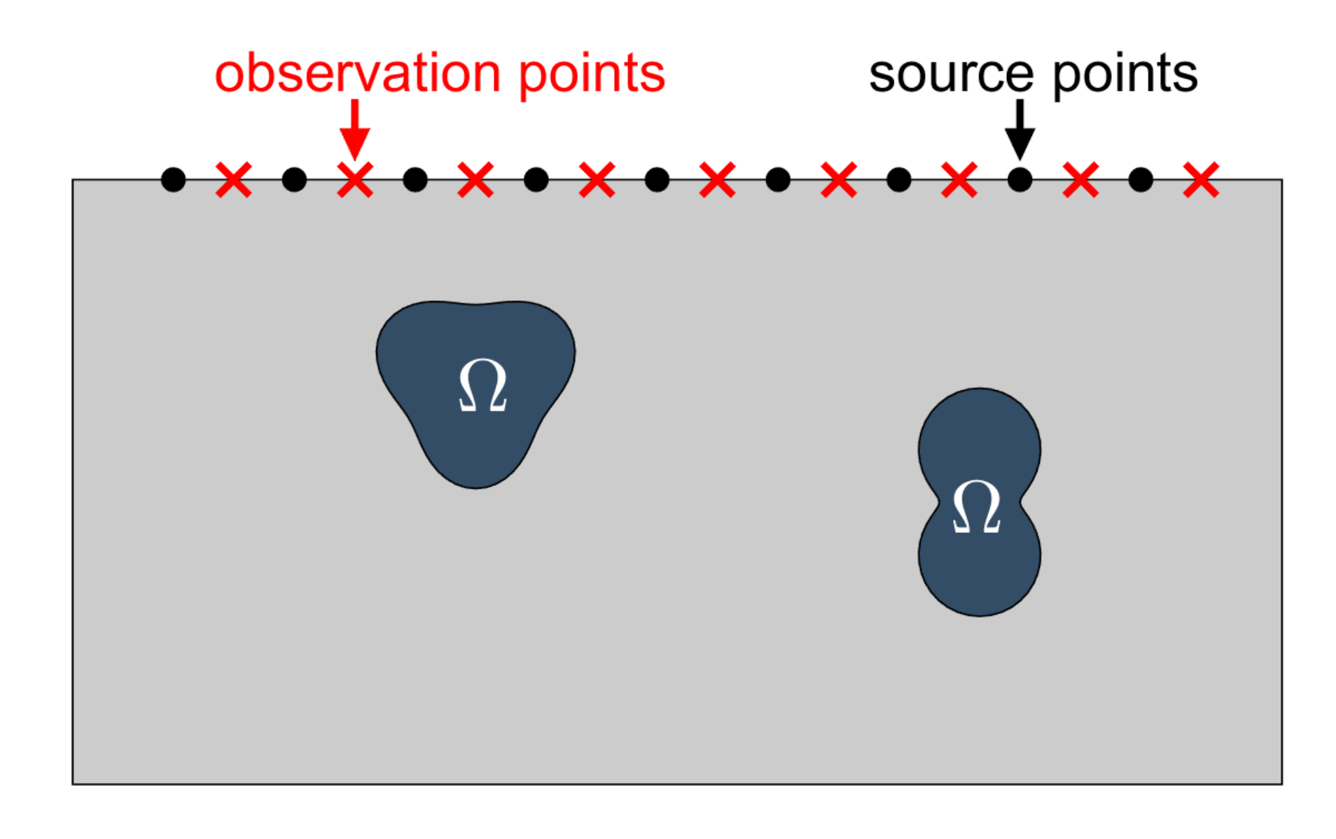
Attenuation complicates the detection of buried scatterers to a great extent. Furthermore, in many applications, data can only be acquired in a limited part of the sounded region, as in seismic tomography or marine acoustics, where taking measurements around the sounded region is impossible. A graphical illustration of such situations is depicted in Figure 1.
A wide variety of algorithms have been proposed to address inverse scattering problems, that is, inverse problems in which the goal is to detect localized objects: linear approximations such as the Kirchhoff or physical optics approximation [5] and the Born approximation [6], linear sampling techniques [7,8], factorization methods [9], backpropagation principles [10], modified gradient methods [11], or single shot methods [12] to quote a few. General shape optimization strategies [13] have inspired many approaches, based, in particular, on level-set methods [14,15] or topological derivative techniques [16,17] (see [18,19] for reviews of recent applications). Here, we show that multifrequency topological derivative-based methods [20,21,22,23] have the potential of providing reconstructions of buried objects in attenuation regimes, within some size and depth limits. We propose a tool based on heuristic ideas, as most of the methods that are based on topological derivatives. For rigorous mathematical justifications of this kind of approach in some specific situations, we refer to [24,25,26].
The paper is organized as follows. Section 2 formulates the forward and inverse scattering problems for penetrable scatterers when both the exterior medium and the objects have nonzero attenuation coefficients. The problem is set in a half-plane (space), but with a symmetry argument, it can be reformulated as a problem in the whole plane (space). Section 3 explains the one-step topological derivative-based method with fixed frequencies, while Section 4 introduces the multifrequency approach. Results are further improved in Section 5, implementing an iterative topological derivative-based multifrequency scheme. Section 6 explains how to extend our method for the detection of sound-soft and sound-hard objects immersed in an attenuating medium. Finally, Section 7 summarizes our conclusions.
2. Forward and Inverse Problems
2.1. Forward Problem
When the incident wave is time harmonic, the resulting attenuated wave field is a time-harmonic solution (where is the excitation frequency), of the damped wave equation
Therefore, the amplitude u is a solution to
where is the wave speed and is the attenuation coefficient. Here the function F (and its time-harmonic amplitude f in the case of time-harmonic excitations) depends on the selected type of incident wave. In the case of time-harmonic planar excitations, , while a point source located at a point is modeled by the Dirac delta function at , .
In the setup depicted in Figure 1, we assume that the components of are penetrable obstacles defined by the wave speed , the attenuation coefficient , and the density . The exterior medium is identified with the half-plane (space) , where or , and described by the exterior parameters . The upper half-plane (space) is assumed to be filled by air, which will be modeled at the upper boundary by the homogeneous Neumann condition
To simplify notations, we introduce the positive ratio
and the complex wave numbers
where the square roots are selected with non-negative imaginary parts.
Incident fields will be generated at points and mathematically described by the fundamental solution of the Helmholtz equation with wave number :
where
being the Hankel function of the first kind and order zero [27]. Notice that since , it follows that satisfies the condition (1). This incident field generates a scattered wave in and a transmitted wave in . The total field
is a solution of
The superscripts + and − denote limit values from outside and inside the objects, respectively. Here, stands for normal derivatives, being the normal unit vector pointing inside the objects, whereas denotes the radial derivative. For our particular type of complex wave-numbers, problem (6) has a unique solution [28] and it can be solved efficiently by means of boundary element techniques [29,30]. In Reference [31] several direct, indirect, and mixed formulations are analyzed and compared for a thermal problem, which has exactly the same structure as (6) but where wave numbers are related to the time-harmonic heat equation and take the form with instead of those in (3). However, for the wave numbers of the form (3), such formulations are also valid. Results in [28,31] are established by using a symmetry argument, where the problem in the half-plane (space) is transformed into an equivalent one in : the condition on disappears and the objects are , where are the original objects and are their symmetrical (with respect to ) ones, namely, . Boundary element methods proposed in [28,31] are based on potentials and operators defined on the symmetric boundary . In the forthcoming examples for the two-dimensional case, we opt for a fully discrete version based on trigonometric polynomials of the direct formulation described in Section 8 in [31] (which indeed is a generalization of the original method proposed in [32]), where the unknowns are the interior and the exterior Cauchy data of the solution of (6) at the boundary of the objects. Alternatively, we could have used the symmetric formulation proposed in [33].
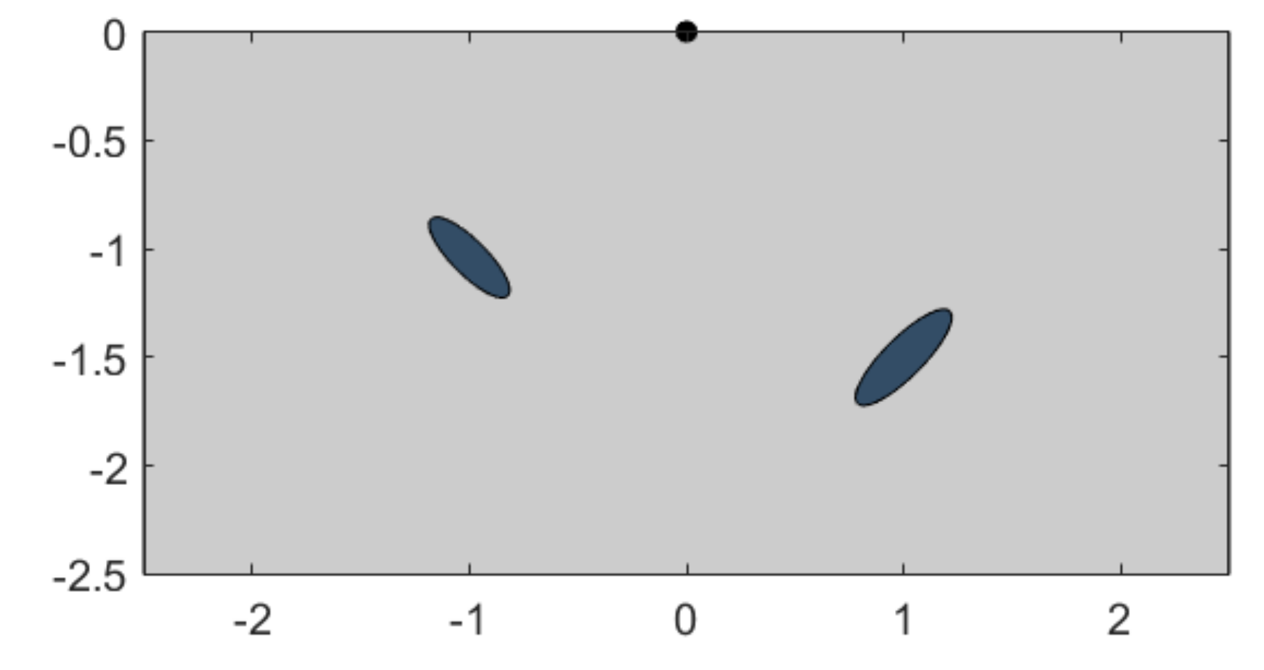
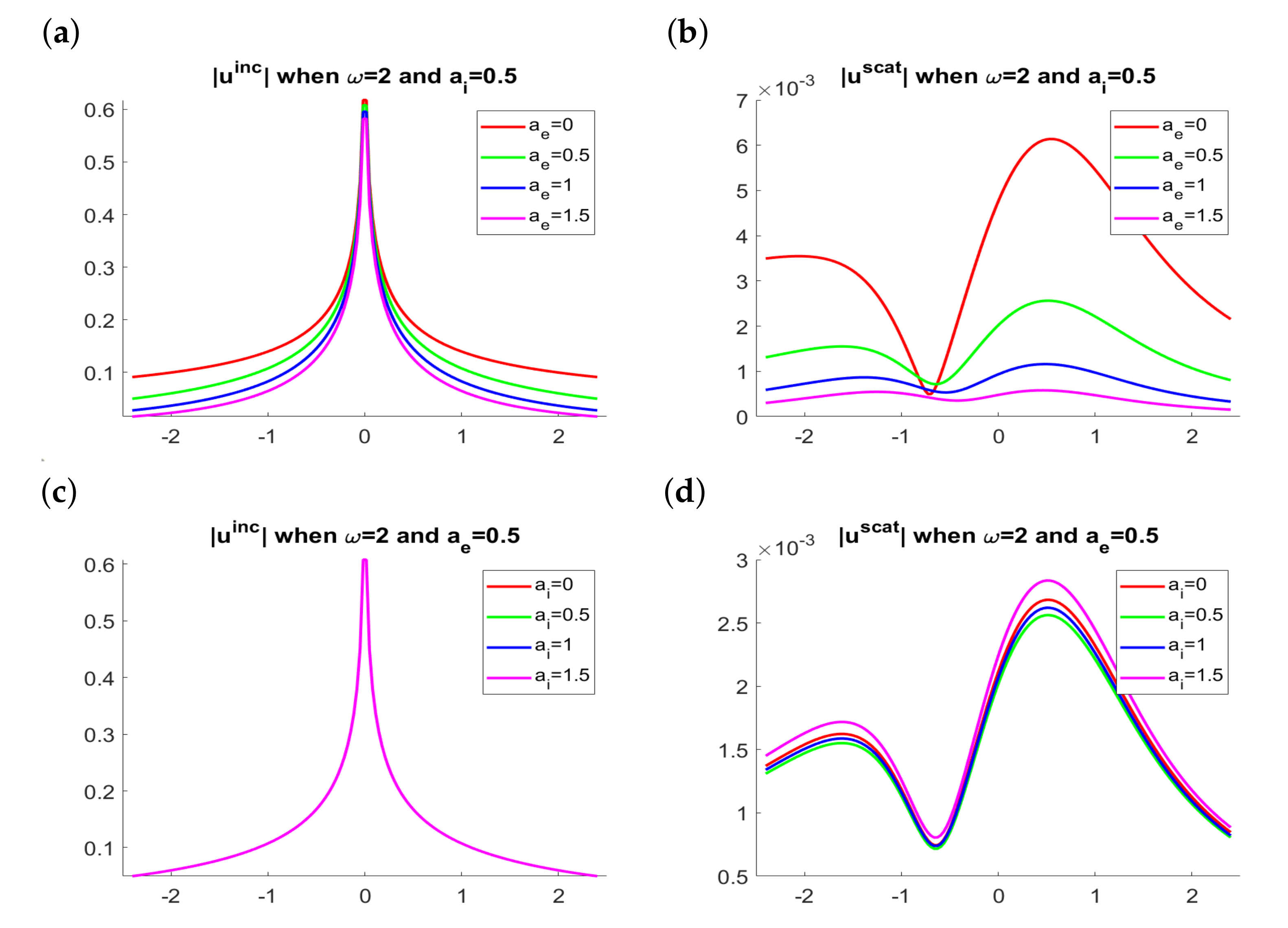
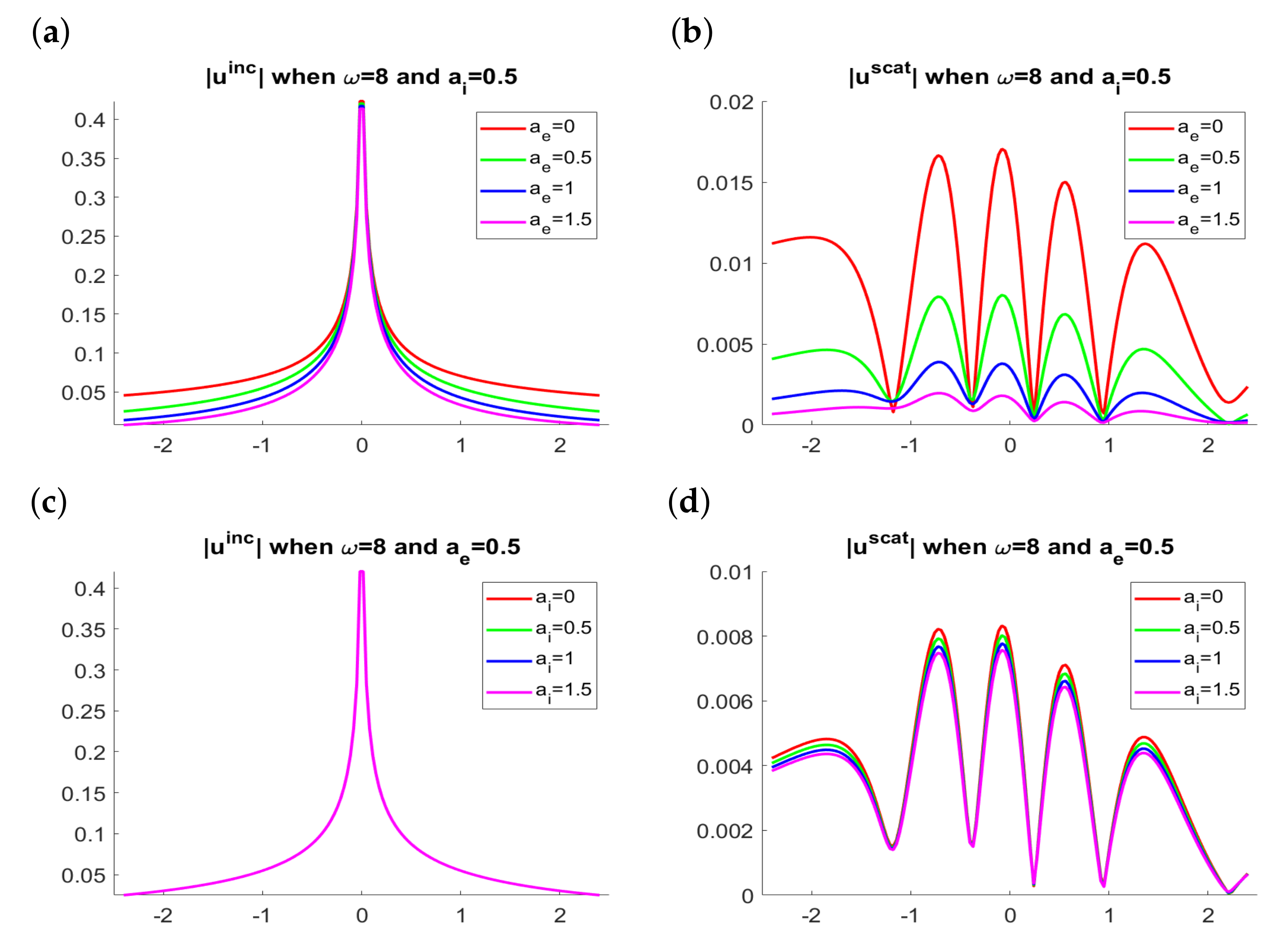
For simplicity, in the initial simulations, we fix , and in the configuration sketched in Figure 2. We will comment on the case in the final simulations. Figure 3 and Figure 4 illustrate the effect of the attenuation coefficients and on the incident and scattered fields for two different frequencies . For a fixed value of the interior attenuation parameter , we observe that the intensity of the scattered waves diminishes as the exterior parameter increases and its maxima are smoothed, while the support of the incident wave becomes smaller. On the other hand, for a fixed value of , the effect of increasing does not have a noticeable qualitative impact on the scattered wave, and of course, the incident wave does not change since it is independent of this parameter. As we increase the frequency , the scattered wave becomes more oscillatory. Notice that the magnitude of the scattered wave depends on the frequency, which will have to be taken into account when combining multifrequency data for shape reconstruction algorithms.
2.2. Inverse Problem
Given objects and the incident wave , the solution of (6) evaluated at the receptors , is expected to agree with the measured data except for measurement errors and noise. When we have measurements of the total wave field at a given frequency for different source point locations , , a constrained optimization reformulation of the inverse problem seeks minimizers of the shape functional
where denotes the solution of (6) with objects for known parameters and when the incident wave is (defined in (4)).
For our two-dimensional experiments, data will be generated synthetically by solving problem (6) for the true defects via the direct formulation described in Section 8 in [31] to obtain the solution at the receivers, , . Then, the associated scattered wave is corrupted by adding a random number of size to generate corrupted scattered values satisfying
Finally, the synthetic measured data are defined by
In the forthcoming experiments, we set a one percent relative noise, namely, . However, we have already checked by numerical tests that results are rather insensitive to and results are almost the same if we consider a ten percent relative noise (i.e., for ). To further avoid inverse crimes, we use a different boundary integral method to solve the direct problems of the form (6) that will appear during the iterative algorithm. Being more precise, we use the indirect formulation described in Section 3 in [31] (see also [28]).
In the next section, we explain how to generate first guesses of the objects by topological derivative methods.
3. Topological Derivative-Based Approach
The concept of the topological derivative was first introduced in the 1990s in [13,34,35] as a tool for optimal shape design. The topological derivative of a shape functional , where and is the solution of a given boundary value problem defined in , is a scalar field that measures the sensitivity of such functional to infinitesimal perturbations at each point . It provides expansions of the form
where are balls of radius centered at and the positive function f satisfies as . The field is the topological derivative of the shape functional at the point . The function f depends on the boundary conditions enforced in the boundary value problem. In our case, and f will be the measure of the ball, that is, when and when . Whenever takes large negative values, the expansion (10) implies that the shape functional decreases by placing an infinitesimal scatterer at . This idea will be exploited in the definition of our reconstruction algorithm.
The general definition of the topological derivative allows for any kind of infinitesimal shape, not necessarily a ball. However, to obtain the associated function f and the derivation of closed-form formulas in this case is more involved, while it is not clear that it would produce improvements in practice, as observed in [36], where a comparison between results for infinitesimal balls and ellipsoids at different orientations is presented for sound-soft and sound-hard objects immersed in a non-attenuating media.
A closed-form expression of the topological derivative of a shape functional similar to (7), involving complex wave numbers, but related to time-harmonic thermal waves in a half-plane is established in [37]. In an acoustic setup in without attenuation, it was established in [36]. In a similar way, we obtain the following result:
Theorem 1.
For any , the topological derivative of the shape functional (7) is
where and solve the forward and adjoint problems with :
and
Both the forward and the adjoint problems can be solved in closed-form (recall that since both emitters and receivers are located on the upper boundary , the fundamental solution satisfies the boundary condition (1) at when is either a receiver or an emitter):
Formula (11) can be directly evaluated in an observation region when the recorded data , the incident waves and the material properties are known. In case the properties of the objects are not known, we can implement iterative procedures to calculate both shapes and material properties following [38]. We will explain how to iterate with respect to the objects using several frequencies in Section 5.
A simpler situation where in the absence of attenuation effects was studied in [36,39]. The formula for the topological derivative is analogous to that in Theorem 1, but the wave numbers and are real. The forward and adjoint problems are similar, but there is no boundary condition on and the forward solution satisfies in , while the adjoint solution solves , in . In this case, when emitters and receivers are distributed around the observation region, the largest negative values of the topological derivative clearly locate the objects for different frequencies, as it happens in Figure 5. The physical parameters selected for this simulation are , and . Notice that the shape and orientation of the two objects are better described when we increase the frequency, in spite of oscillations.
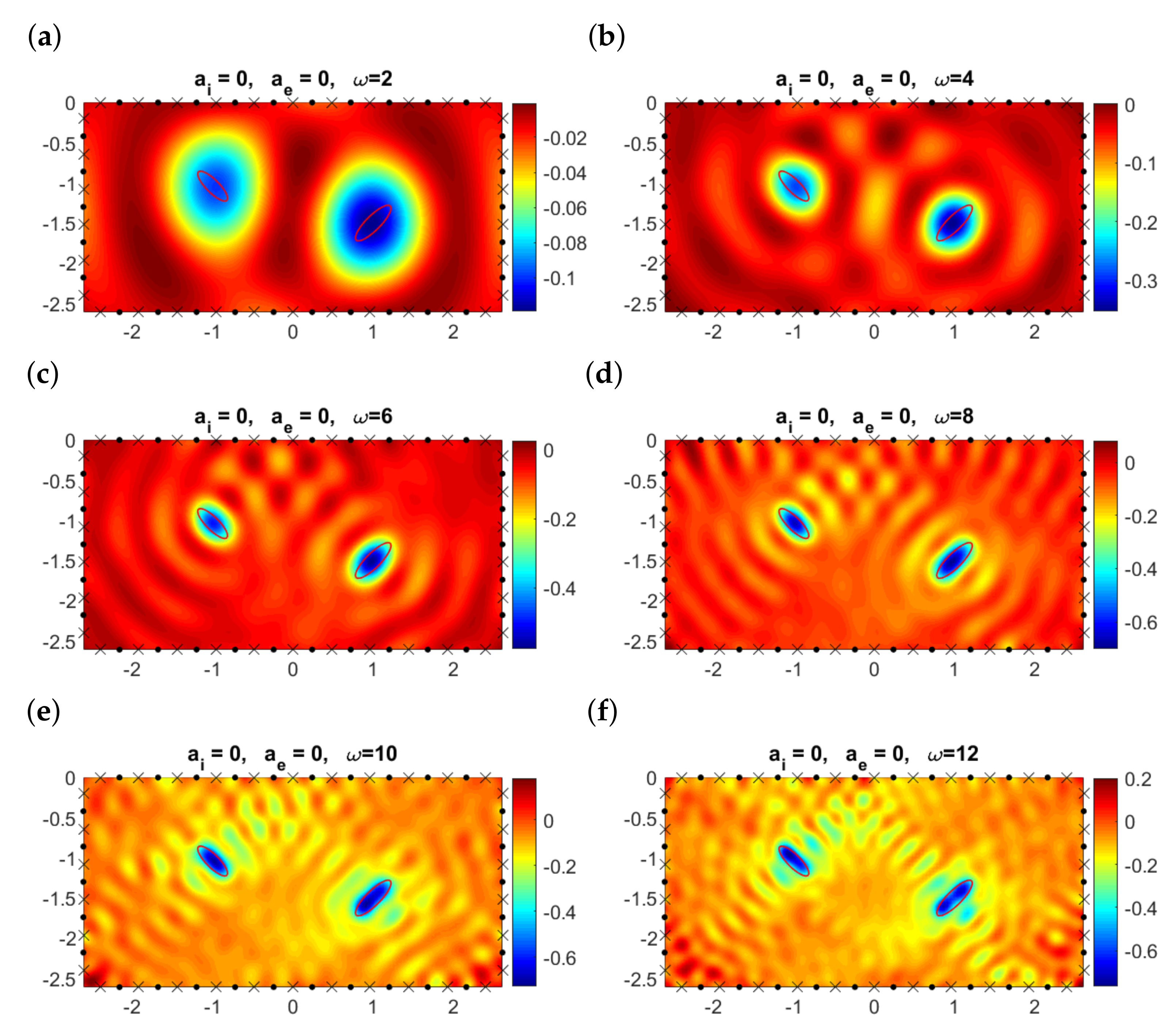
Let us turn now to the original problem set in for the limited aperture configurations under study, see Figure 1. Locating buried scatterers with limited-aperture data is an issue of practical interest that has been the object of intensive research [36,40]. Placing emitters and receivers on the upper boundary, and keeping the same physical parameters , , and , the information provided by topological derivatives is less clear, as illustrated in Figure 6. Now, we observe stripes alternating positive and negative values of the topological derivative. Nevertheless, the largest negative values are attained around the two true objects, though resolution for the object placed farthest from the emitters worsens, especially as the frequency increases. In comparison with the experiments presented in Figure 5, we observe that while frequencies are the best for shape identification when emitters and receivers are located around the objects, in our setting with emitters and receivers on , the use of frequencies higher than promotes the appearance of spurious regions. Only frequencies below will be considered in the forthcoming experiments. If we increase the number of emitters and/or receivers but we keep their location on , reconstructions do not improve.
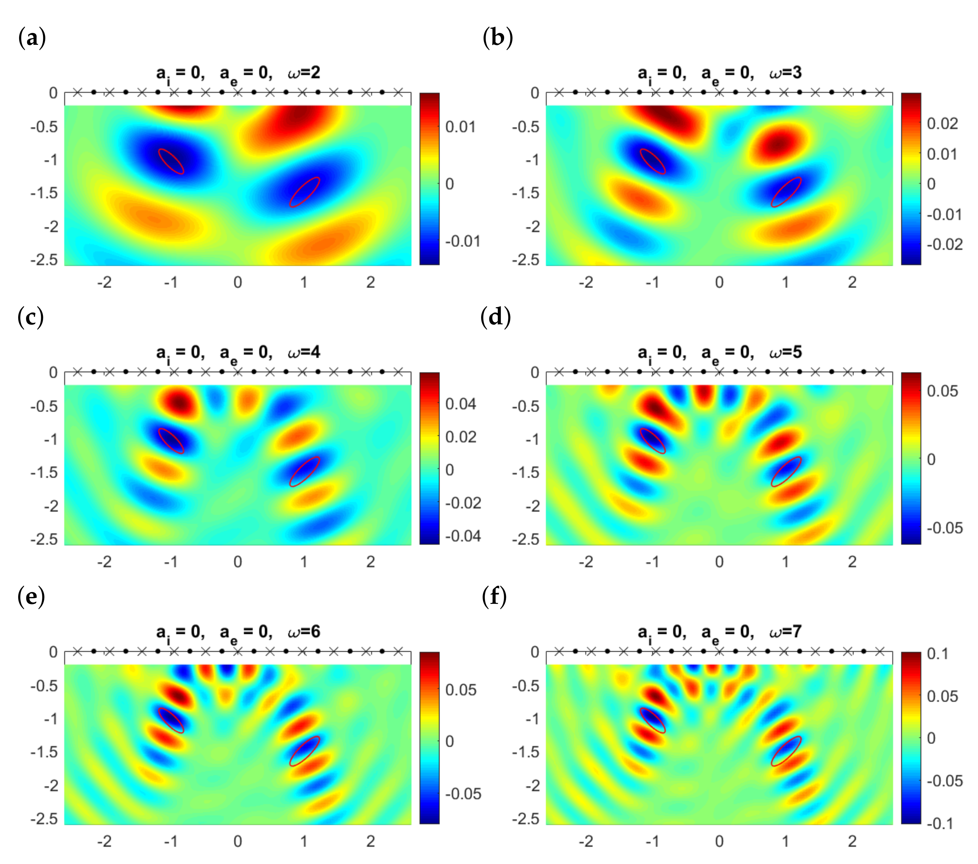
In the presence of attenuation, we lose even more information, see Figure 7 where . The topological derivative still detects the closest object, though its orientation is uncertain. We fail to detect the distant object, while a number of spurious minima appear. Depending on the frequency, we may end up with completely wrong reconstructions. For instance, for , we conjecture the presence of a close object at about , whereas for , we seem to have three defects. If we increase the interior attenuation coefficient to and keep , the topological derivatives are qualitatively equal to those presented in Figure 7 and therefore plots are omitted for brevity.
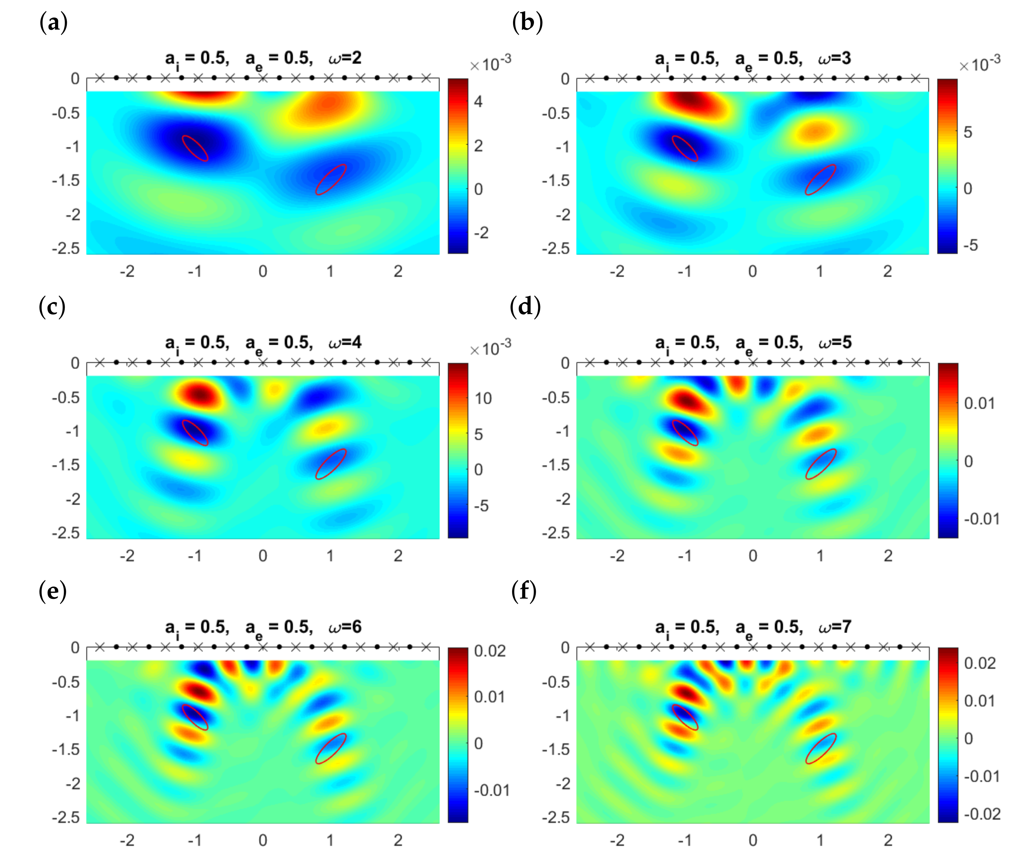
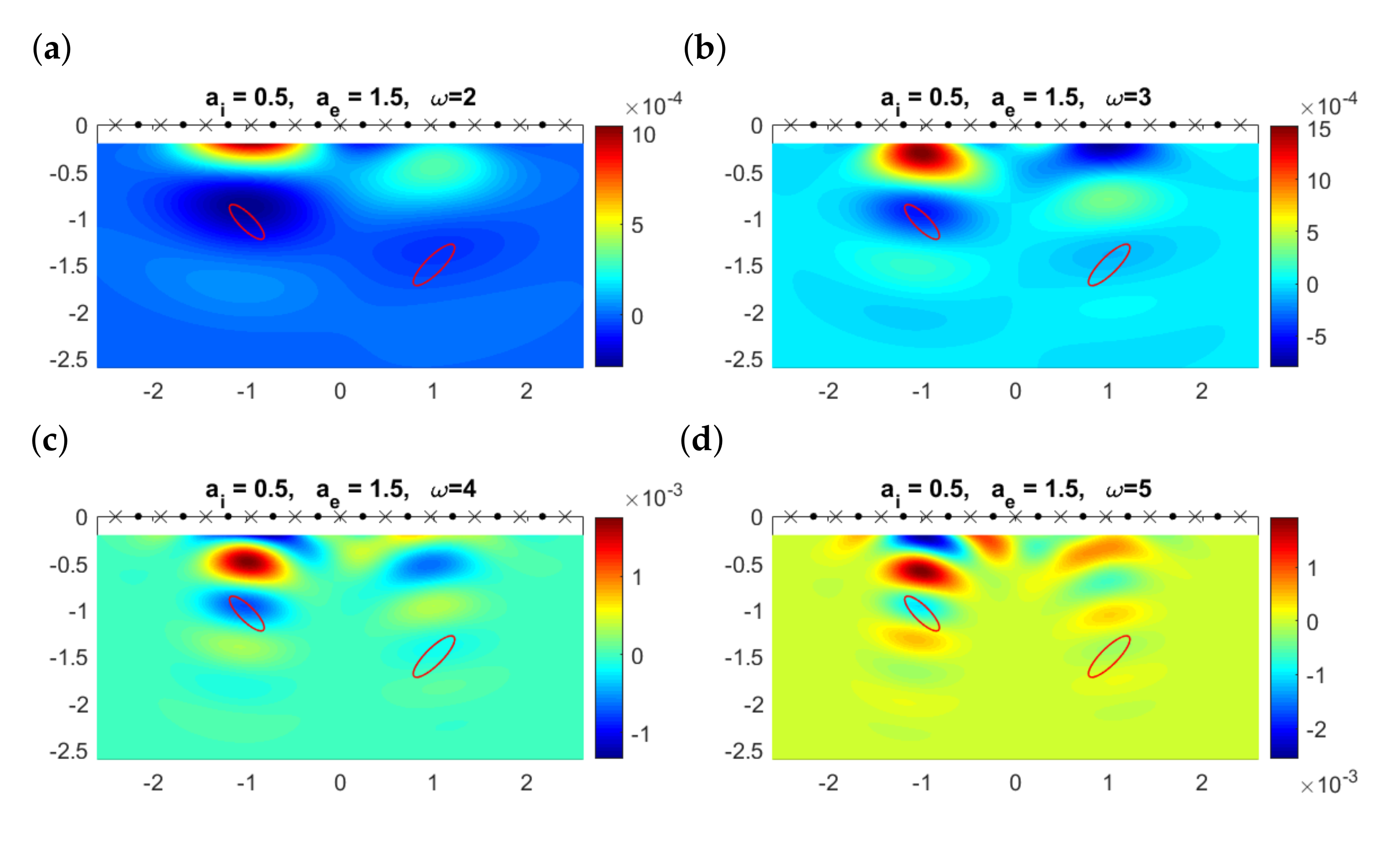
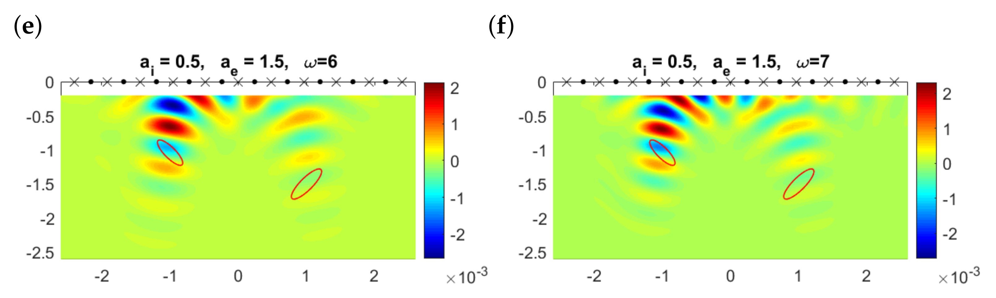
Further increasing the exterior attenuation coefficient to while keeping the interior one unchanged (or increasing it to ), reconstructions worsen. As shown in Figure 8, only the lowest frequency can track the closest object. The true objects are usually placed in regions where the topological derivative takes negative values, but the largest negative values are attained in variable regions as the frequency changes. Furthermore, there are regions where large negative values for one frequency become large positive values for another (compare panels (c) and (f), for instance). These remarks suggest the possibility of combining information from different frequencies to enhance the correct contributions provided by all of them and to cancel the variable, spurious details, which we analyze in the next section.
4. Multifrequency Method
To incorporate the contributions from several frequencies , we consider a new shape functional defined as a linear combination of monochromatic functionals (7), namely, a function of the form [22]:
where is the solution of (6) with frequency and incident wave of the form (4). Here, are weights to be selected. By linearity, it follows that the topological derivative is a linear combination of the monochromatic topological derivatives with given in (11), i.e.,
As in [22], we select the weights after computing each individual derivative, selecting
where is the observation region, that is, the region where topological derivatives are evaluated. This choice balances the contribution of all frequencies since it guarantees that each term in the sum (17) satisfies . Notice that depending on the selected frequency, has a different order of magnitude (compare panels (a) and (f) in Figure 6, Figure 7 and Figure 8).
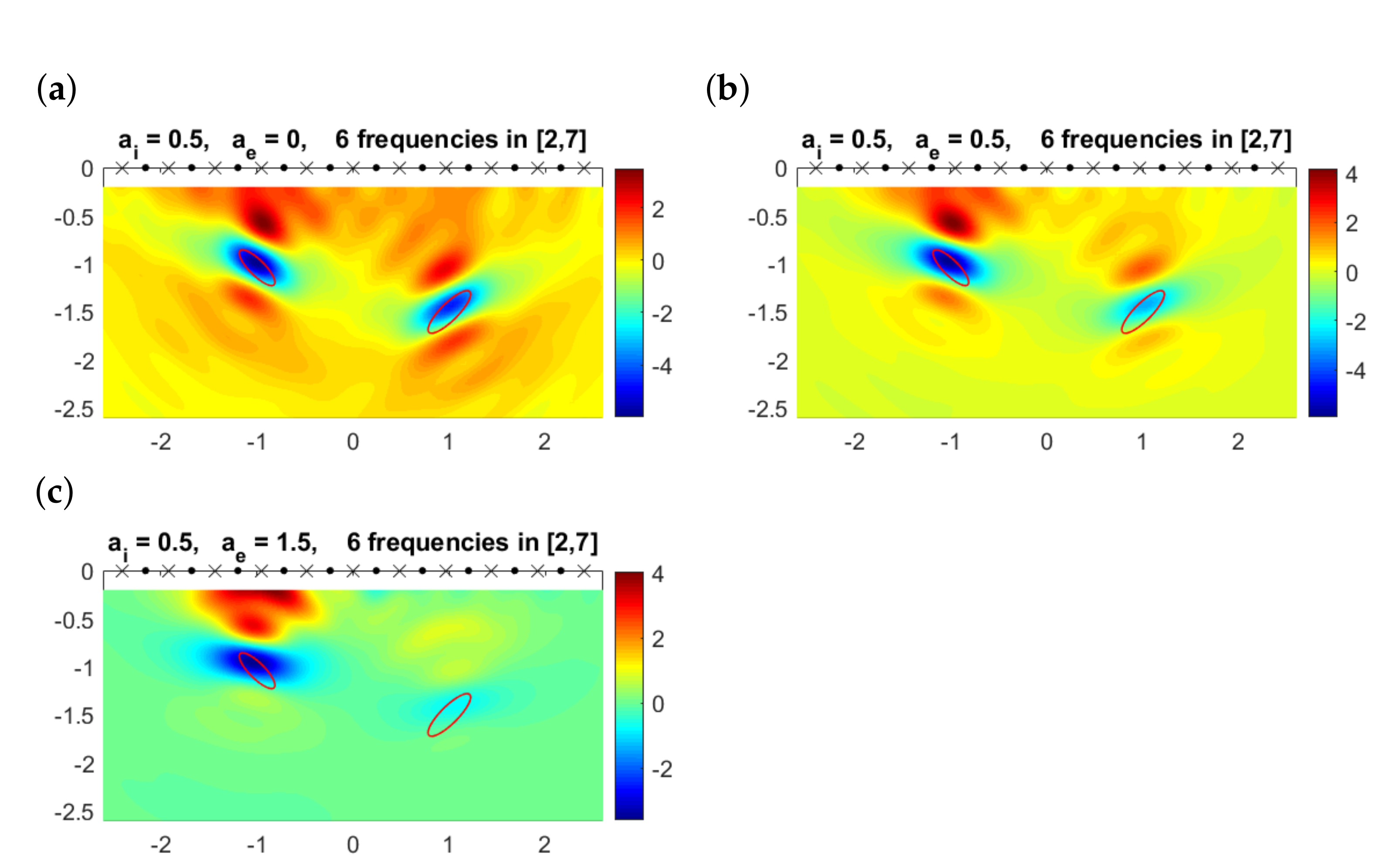
Figure 9 illustrates the results obtained combining the six single frequency topological derivatives for the same ellipses () when the exterior velocity is and (no exterior attenuation), (moderate attenuation) and (high attenuation). For the attenuation coefficients and , we have combined the six topological derivatives displayed in Figure 7 and Figure 8, while for the individual ones are qualitatively identical to those in Figure 6, which corresponds to instead of . When , we clearly distinguish two elliptical defects, obtaining good approximations for their size, shape and orientation. For , the object closest to emitters/receivers is reasonably reproduced, similarly to the case , but the orientation slightly worsens. We conjecture the presence of another object in the second region where the multifrequency topological derivative becomes negative, and no spurious negative regions where no true objects are located appear. Increasing the attenuation in the medium, the information on the orientation of the closest object worsens and the other object cannot really be guessed.
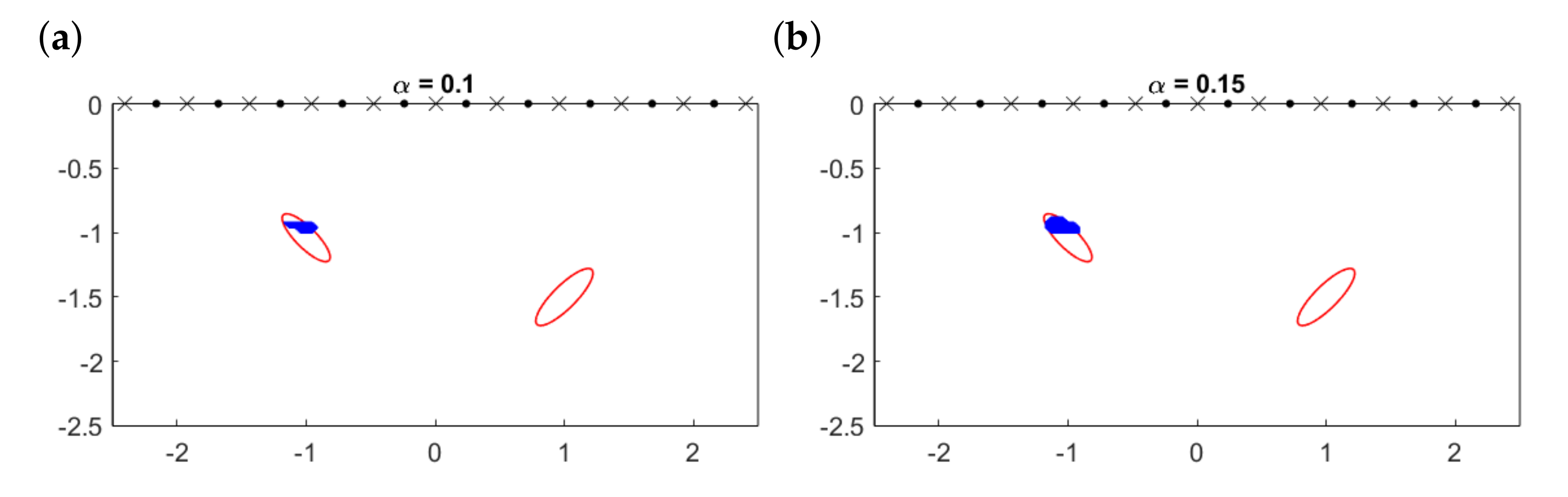
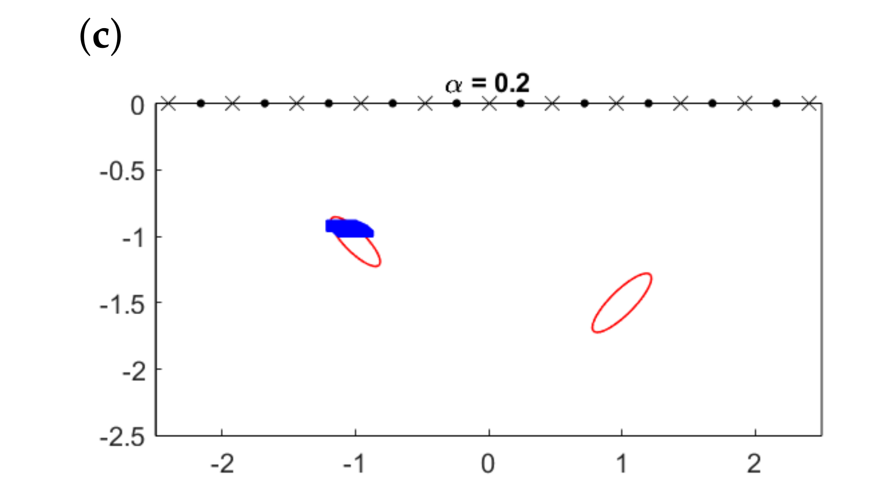
For a quantitative visualization, Figure 10 illustrates the initial approximations we would obtain plotting the topological derivative (17) for the example in Figure 9c (which corresponds to the most demanding case ) and selecting the points for which the topological derivative falls below a threshold:
where is the selected threshold coefficient and is the sounded region. Obviously, the larger , the larger the area. However, notice that reconstructions are robust in terms of this parameter and only a rough calibration is needed. Notice also that not only depends on but also on the selected mesh for (both for the definition of each weight , and for the final evaluation of the multifrequency topological derivative). In all our experiments, we have considered a grid of 120 points in the x-coordinate and 60 points in the y-coordinate. We have also checked that the method is very robust in connection with this issue. For a discussion about the selection of optimal meshes for the evaluation of indicator functions, we refer to [41].
These results provide the initial stage to implement iterative corrections, as we explain in Section 5.
5. Multifrequency Iterative Method
In this section, we adapt the iterative algorithm proposed by us in [37,39] for monochromatic measurements to the multifrequency case. It is based upon an expression of the topological derivative when we already have a non-empty guess for the scatterers.
Theorem 2.
Assume that is an approximation of the true defects Ω. Then, for any the topological derivative of the shape functional defined in (7) is given by
where and are solutions of forward and adjoint problems with objects :
and
Notice that Formulas (11) and (20) are exactly the same, but now and play the role of their counterparts and in Theorem 1. In contrast to the former case, problems (21) and (22) cannot be solved in closed form except for very simple geometries (i.e., when is a ball or a square), and they must be solved numerically. This will be the general situation for the initial guesses defined by (19). As already mentioned, we will use the indirect boundary integral formulation proposed in [28].
The iterative method we propose to approximate the true objects from knowledge of the physical parameters and from measured data for , , corresponding to the excitation of the medium via incident waves , is a multifrequency version of the one proposed by us in [37,39]. The algorithm proceeds in the following steps:
- Initialization. We initialize the method by computing the multifrequency topological derivative defined in (17) from the individual ones (as described in Theorem 1) with weights defined by (18). Then, we select a value and define the setFor our numerical experiments, we will set in principle . For numerical purposes, the set needs now to be decomposed in its connected components, which is performed by using the Matlab function bwconncomp as explained in [42], and then each connected component is approximated by a star-shaped parameterization as detailed in [39].
- Iteration. For each step we proceed as follows. Given the current approximation ,
- -
- We compute the monocromatic topological derivatives for making use of Theorem 2 with , to define the new multifrequency topological derivative:with weights . Notice that now the corresponding forward and adjoint problems involve the objects and therefore they have to be numerically solved.
- -
- We update the current set by adding to the points where the new topological derivative attains the largest negative values:In principle, . We calculate the number of connected components of and obtain star-shaped approximations of each of them, which form the final .
- -
- We check if each monofrequency shape functional decreases. If for , then is accepted. Otherwise, we replace by and compute again as in (24). The algorithm stops if either:
- *
- A maximum number of iterations is reached.
- *
- The measure of two consecutive approximations is negligible, namely if
- *
- Updating objects produces almost no variation for all the monofrequency functionals, i.e., if
- *
- The discrepancy principle for at least one of the frequencies is reached, that is, for anywhere is the noise level (see the end of Section 2.2).
Notice that since , at each step we are considering a different shape functional, which is a different linear combination of the same monochromatic functionals. In our previous works, only monochromatic data were considered, and therefore, the same shape functional was preserved during the iterations. As stated, this iterative procedure only allows us to create objects and add points to existing objects. Modifying the iterative scheme as indicated in [43], we can also remove points or destroy existing spurious components.
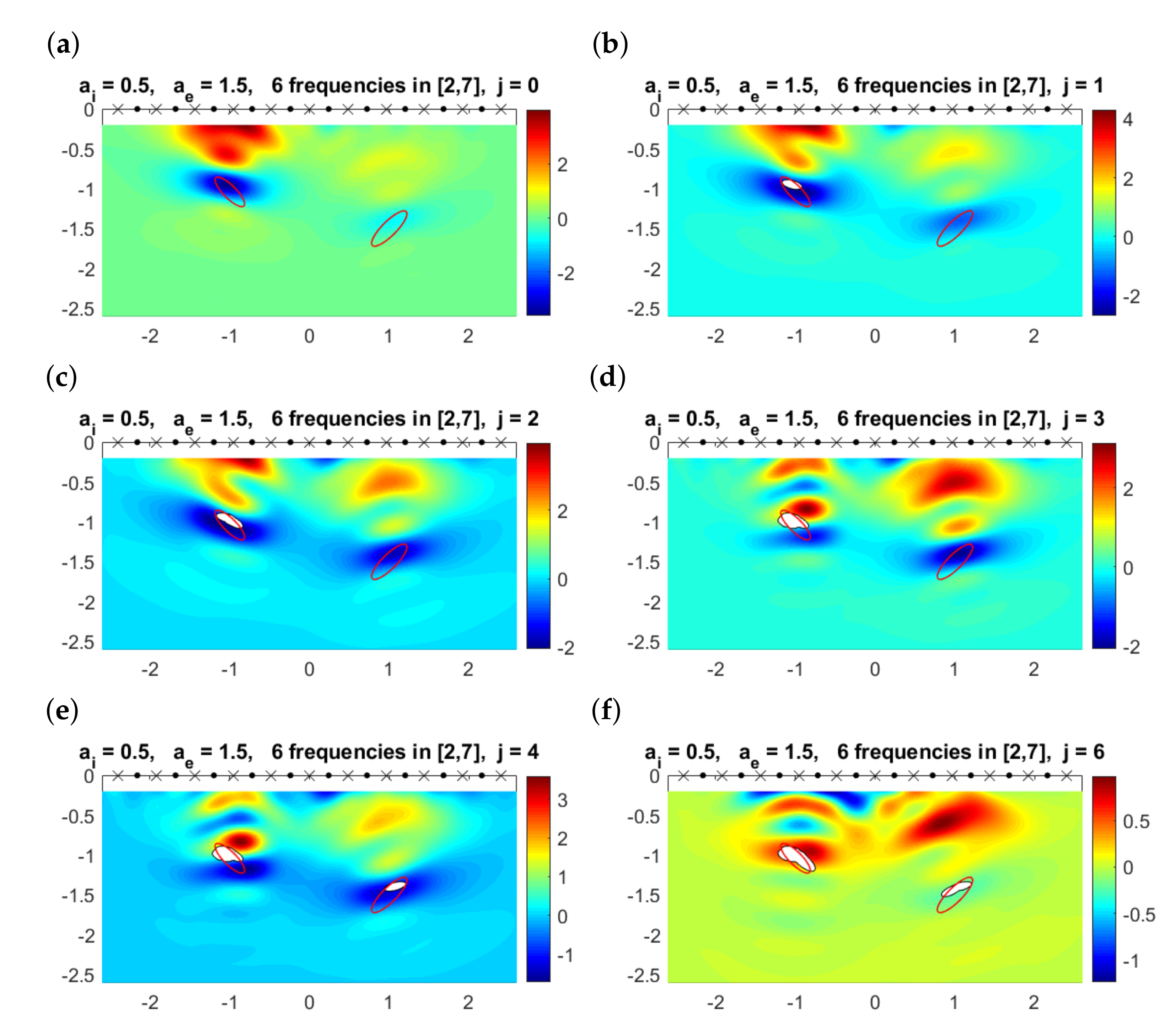
Next, we will illustrate the performance of the iterative multifrequency algorithm for the two-dimensional case. Figure 11 shows how the iterative method works for the demanding situation considered in the previous section where and . Plot (a) represents the values of the topological derivative for computed as in Theorem 1. Choosing , we find the initial approximation shown in panel (b) in white. In the same plot, we represent the values of the topological derivative when computed by applying Theorem 2. The subsequent plots, indexed by the value of j in the title, represent the current approximation and the values of the topological derivative when (which are used to define by Formula (24)). We observe that although our initial guess contains only one component, the second one is detected when and has the correct number of components. In fact, the topological derivative for already suggests it, but since the value of is rather conservative, the approximate domain has only one component. The last approximation to the closest object is quite good (see panel (f)), including size, shape and orientation. For the deepest one, the location is correct, though it appears smaller. We only see the top illuminated part.
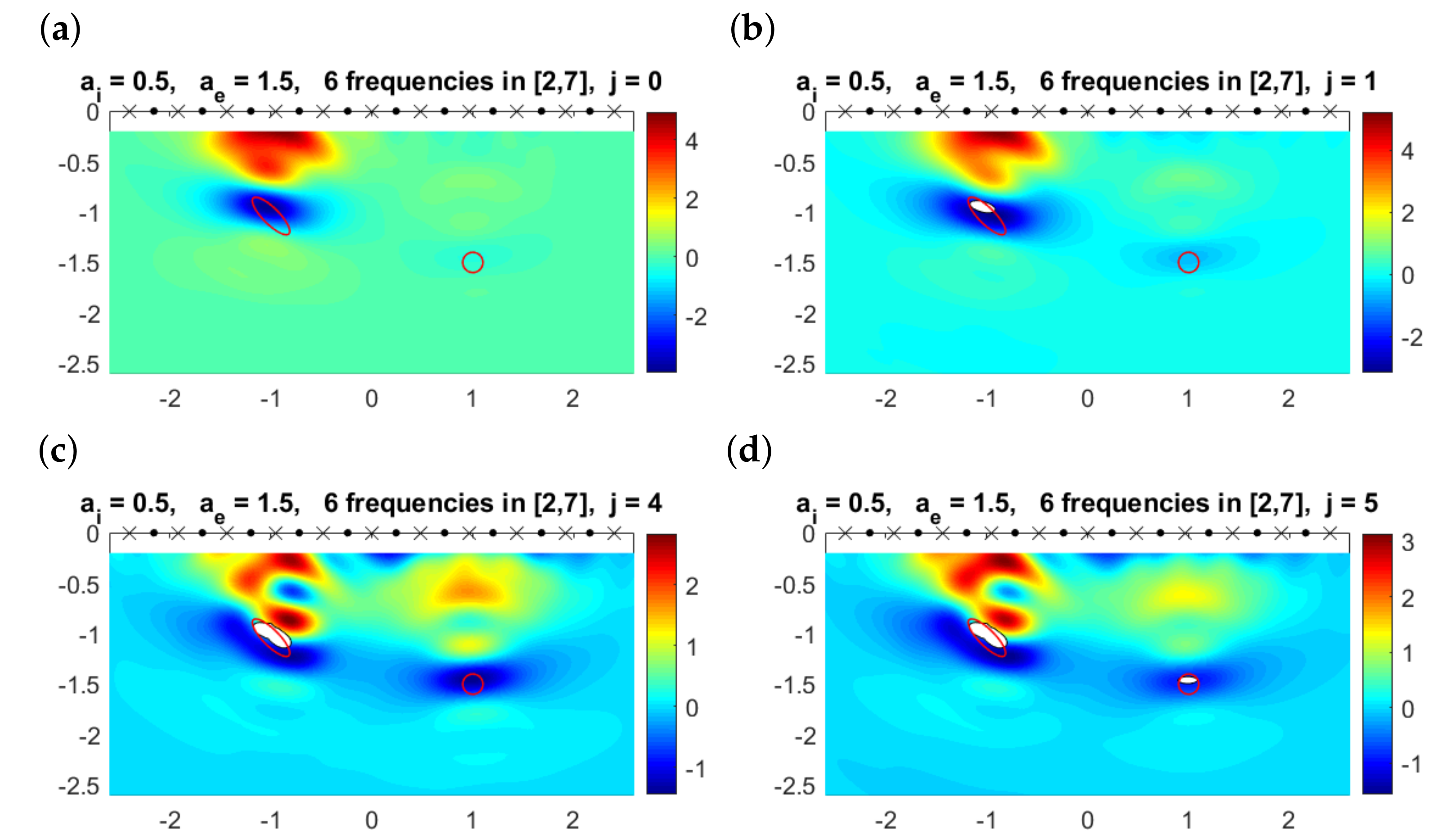
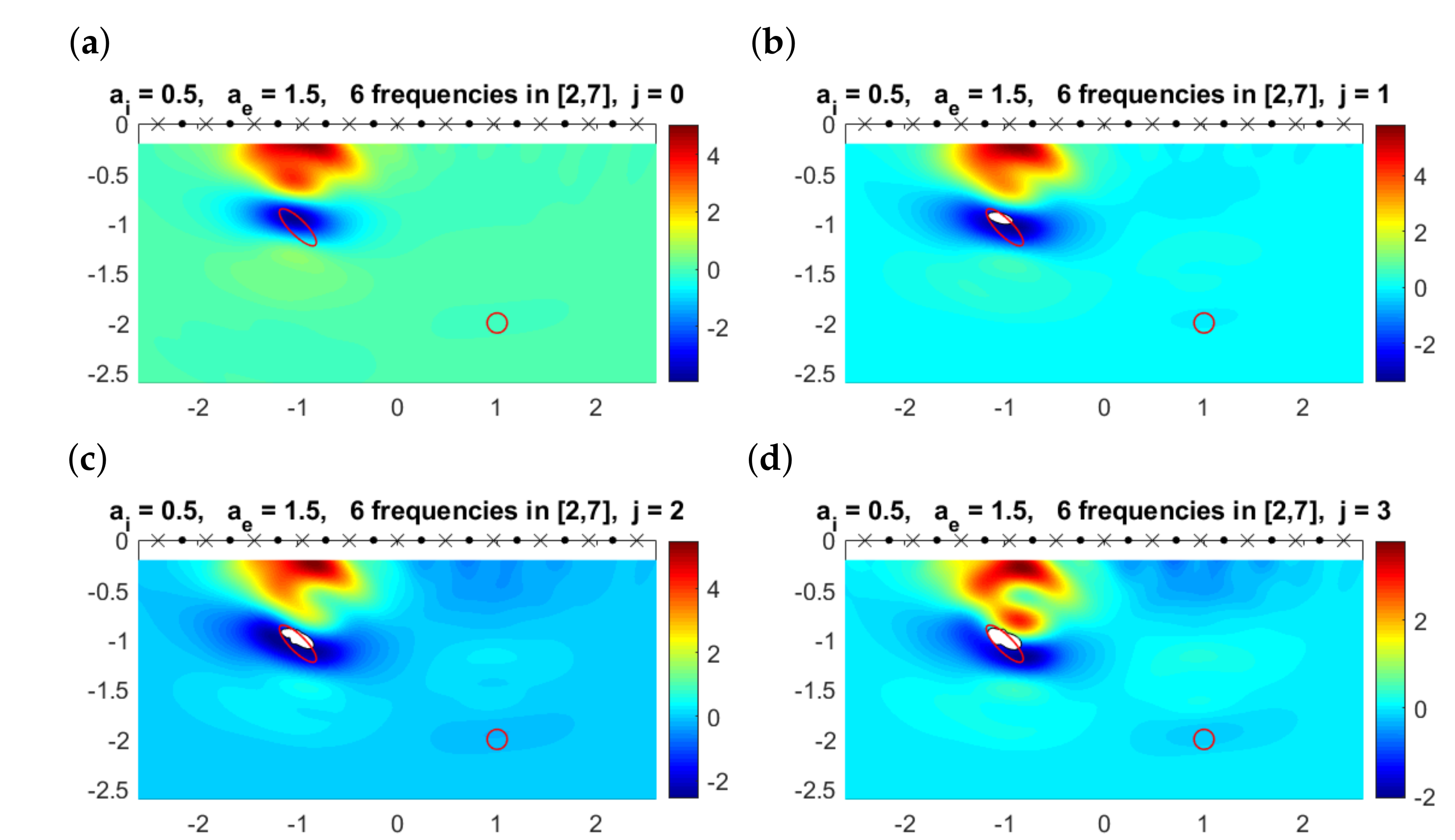
Figure 12 considers a more challenging situation: the deepest object is smaller and deeper. However, our method is also able to detect it. As we move this object deeper, we reach a depth at which we do not see it with our choice of frequencies, attenuation and thresholds, as can be seen in Figure 13. Nevertheless, the other object is still reasonably described. Attenuation effects hinder the detection of objects, when they are deep and small enough.
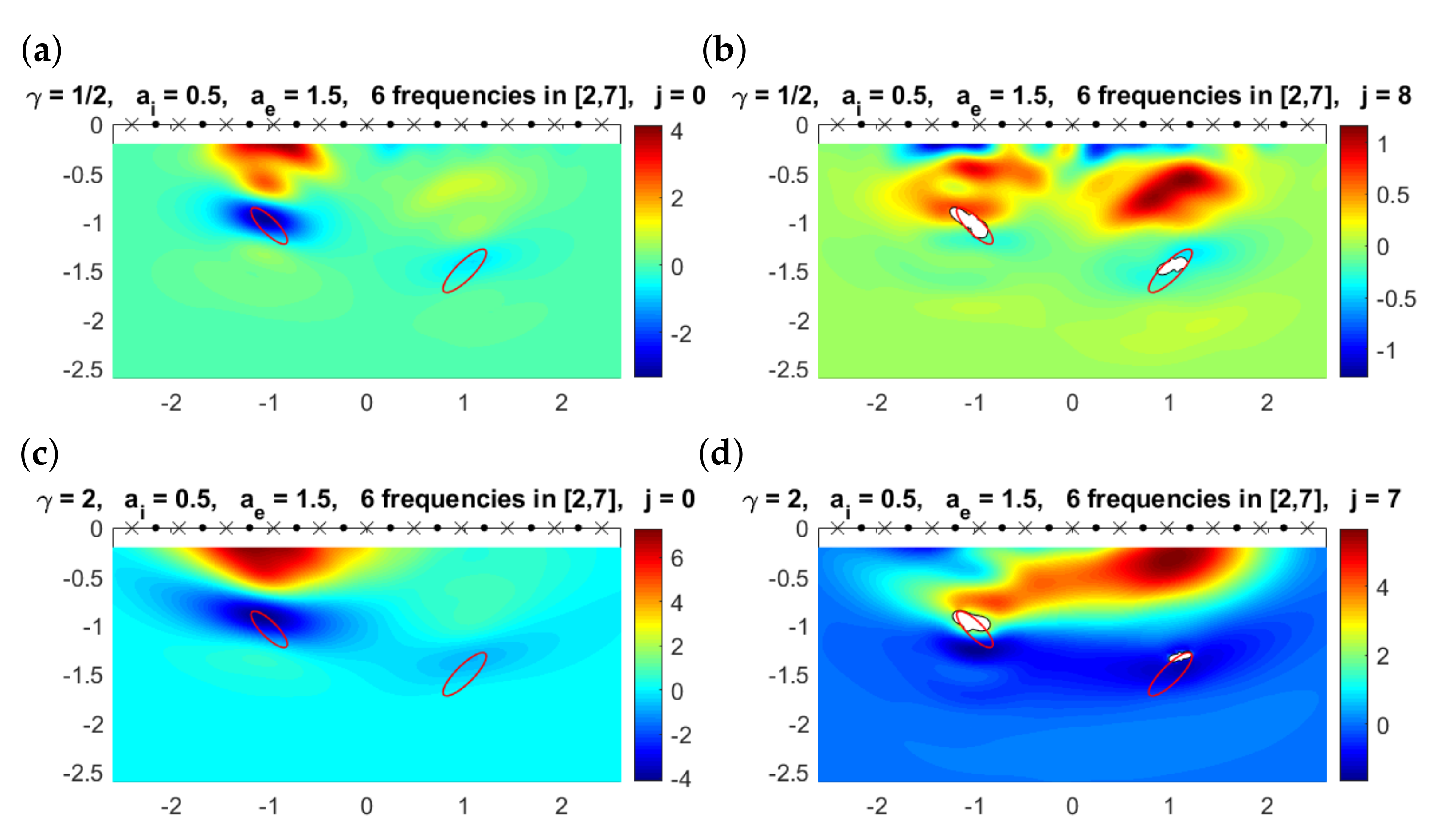
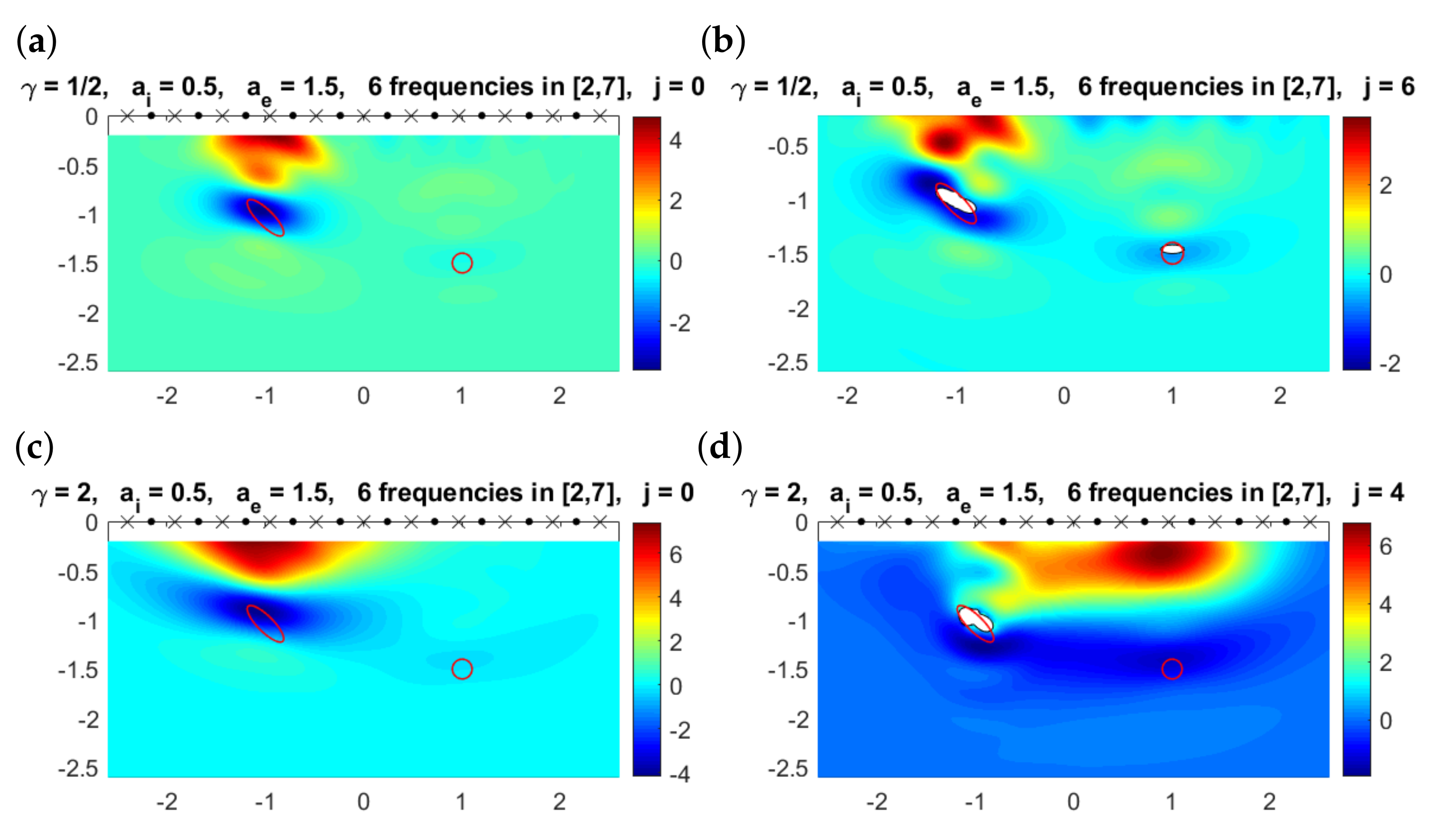
In all previous examples, the physical parameters , and were fixed. Since in realistic situations that appear, for instance, in geophysics or in biological problems [44], the simplification could be unrealistic, we have repeated the experiments in Figure 11 and Figure 12 when replacing by and . Figure 14 shows the results for the configuration with two ellipses, and Figure 15 corresponds to the configuration where the deepest object is a ball.
Results evidence that the effect of attenuation is similar in the cases , and , being the case the one that seems to be less favorable. In particular, in Figure 15d, we observe that the small defect is not detected when . Although not illustrated here for brevity, when considering the configuration in Figure 13, in all of the cases (, and ) the deepest object is missed. We want to emphasize that we have not performed a thorough parametric study and it might happen that for other selections of speeds and frequencies, the case could lead to more accurate reconstructions than or .
Finally, let us remark that topological derivative-based methods are very robust with respect to noise. This has been extensively tested by many authors for different inverse problems (see for instance [17,20]). Synthetically generated data are usually corrupted by random noise in a similar way as we do in (8) and (9). When real experimental data are processed, noise is inevitably present. The reconstructions obtained in [23,45] evidence the robustness of the method when dealing with experimental data. For our inverse scattering problem in an attenuating half space, we have checked that increasing the level of noise defined in (8) from to results are almost identical. A detailed study of the effect of noise on a topological derivative-based approximation is performed in [46] in a Bayesian framework, though it is exemplified in different emitter/receiver configurations.
6. Other Boundary Conditions
The ideas developed in this paper do not depend on the conditions on the boundary of the defects. The results can be extended straightforwardly to Dirichlet (sound-soft defects) or Neumann (sound-hard defects) conditions. For sound-soft defects embedded in an attenuating media occupying the half plane/space , the counterpart forward problem corresponding to (6) for an incident wave emitted from the source point at a frequency is:
where the complex wave number is defined in terms of the exterior wave velocity and the attenuation coefficient as in (3). In this case, adapting the results in [47,48,49] it can be proved that the formula for the topological derivative in Theorem 1 should be replaced by:
where and solve (12) and (13). In case an initial guess of is available, we obtain the counterpart formula to (26) with and replaced by and , and the solutions to the associated Dirichlet forward and adjoint problems with objects :
and
These formulas can be derived by adapting the results in [49].
For sound-hard objects, modeled by the analogous problem to (25) obtained by replacing in this problem the boundary condition on by on , the counterpart formula to that in Theorem 1 can be obtained either by adapting the results in [17,39] or by formally taking the limit as in (11):
where again, and solve (12) and (13). The counterpart formula to that in Theorem 2 looks exactly as (29), with and replaced by and , the solutions to the associated Neumann forward and adjoint problems with objects . The forward problem is (27) with the condition on replaced by on , while the adjoint problem is given by (28) when replacing on by the Neumann condition on .
Notice that for the three types of defects (penetrable, sound-soft and sound-hard), the same forward and adjoint problems are involved in the topological derivative Formulas (11), (26) and (29). However, depending on the type of defect, the formulas are different linear combinations of the terms and . In the case of not having information about the nature of the scatterers (and even in the case when objects of different nature are embedded in the same attenuating media), we could make use of a related mathematical tool, the topological energy [50], which for our model problem would be defined by
where and solve (12) and (13). For the use of a multifrequency version of this indicator function for a problem in where objects of different nature are immersed in a non-attenuating media, we refer to [51]. The extension of the iterative method to cope with objects of different nature is not immediate, since the formula would be the counterpart to (30), but the corresponding fields and depend on the boundary conditions imposed on the components of . Therefore, at its current state, we could only generalize the use of iterated multifrequency topological energies to the situation where all objects have the same nature. A monofrequency iterative method based on topological energy computations was explored in [52] for a related problem in with no attenuation and penetrable objects.
7. Conclusions
We have proposed a topological derivative-based multifrequency iterative algorithm to identify objects buried in attenuated media with limited aperture data. In principle, these methods use no a priori information other than the knowledge of the measured data, the incident waves, the employed frequencies and the properties of the background medium. To simplify, here we have assumed that we know the material properties of the scatterers, and we look for their location, size, orientation and shape. One-step implementations of the algorithm provide initial approximations, which are improved in a few iterations. Components of smaller size than the main components, or buried deeper inside, can be detected. However, attenuation effects may prevent detecting objects depending on their size and depth for fixed ranges of frequencies.
A key point in the new multifrequency method defined in this paper is the way to combine monochromatic data. We have defined a strategy based on weighting individual topological derivatives, obtaining therefore a method where the global shape functional changes from one step to the next one, and consequently, the discrepancy principle must be tested individually. It would be possible to define the weights in a different way to keep the same functional or to define a different way to combine single-frequency data in a more efficient way, exploring the alternatives proposed in [21,53,54,55,56]. Indeed, the weights could be considered part of the inverse problem. Optimal selection of weights could extract more information from the measured data, perhaps increasing resolution of small deep objects.
The formulas obtained in this paper could be combined with other strategies to define iterative methods. For instance, the reconstructions obtained by the first computation of the topological derivative in could be used as initial guesses for other types of iterative methods, such as Newton-type algorithms [57], level set methods [14,15] or other topological derivative-based approaches [58,59,60,61,62]. Iterative methods that alternate topological derivative computations with regularized Gauss-Newton iterations [63] could also be explored.
When the material properties of the objects are unknown, we could generate initial approximations to their geometry by related topological energy techniques [45,50,51,52] and to their material parameters by hybrid gradient methods [38]. Uncertainty due to noise can be addressed by combining topological priors with Bayesian techniques [46].
Author Contributions
Investigation, A.C. and M.-L.R. All authors have read and agreed to the published version of the manuscript.
Funding
This research was founded by Spanish FEDER/MICINN-AEI grants MTM2017-84446-C2-1-R, PID2020-112796RB-C21 and PID2020-114173RB-I00.
Conflicts of Interest
The authors declare no conflict of interest.
References
- Jones, J.P.; Leenman, S. Ultrasonic tissue characterization: A review. Acta Electron. 1984, 26, 3–31. [Google Scholar] [CrossRef] [Green Version]
- Gaikovich, K.P.; Gaikovich, P.K.; Khilko, A.I. Multifrequency near-field acoustic tomography and holography of 3D subbottom inhomogeneities. Inverse Probl. Sci. Eng. 2017, 25, 1697–1718. [Google Scholar] [CrossRef]
- Roitner, H.; Burgholzer, P. Efficient modeling and compensation of ultrasound attenuation losses in photoacoustic imaging. Inverse Probl. 2011, 27, 015003. [Google Scholar] [CrossRef]
- Agaltsov, A.D.; Hohage, T.; Novikov, R.G. Global uniqueness in a pasive inverse problem of helioseismology. Inverse Probl. 2020, 36, 055004. [Google Scholar] [CrossRef] [Green Version]
- Liseno, A.; Pierri, R. Imaging of voids by means of a physical optics based shape reconstruction algorithm. J. Opt. Soc. Am. A 2004, 21, 968–974. [Google Scholar] [CrossRef] [Green Version]
- Devaney, A.J. Geophysical diffraction tomography. IEEE Trans. Geosci. Remote Sens. 1984, 22, 3–13. [Google Scholar] [CrossRef]
- Colton, D.; Gieberman, K.; Monk, P. A regularized sampling method for solving three dimensional inverse scattering problems. SIAM J. Sci. Comput. 2000, 21, 2316–2330. [Google Scholar] [CrossRef] [Green Version]
- Colton, D.; Kirsch, A. A simple method for solving inverse scattering problems in the resonance region. Inverse Probl. 1996, 12, 383–393. [Google Scholar] [CrossRef]
- Kirsch, A. Characterization of the shape of a scattering obstacle using the spectral data of the far field operator. Inverse Probl. 1998, 14, 1489–1512. [Google Scholar] [CrossRef]
- Natterer, F.; Wubbeling, F. A propagation backpropagation method for ultrasound tomography. Inverse Probl. 1995, 11, 1225–1232. [Google Scholar] [CrossRef]
- Kleinman, R.E.; van der Berg, P.M. A modified gradient method for two dimensional problems in tomography. J. Comput. Appl. Math. 1992, 42, 17–35. [Google Scholar] [CrossRef] [Green Version]
- Li, J.; Liu, H.; Zou, J. Locating multiple multiscale acoustic scatterers. Multiscale Model. Simul. 2014, 12, 927–952. [Google Scholar] [CrossRef]
- Sokolowski, J.; Zolésio, J.P. Introduction to Shape Optimization. Shape Sensitivity Analysis; Springer: Berlin/Heidelberg, Germany, 1992. [Google Scholar]
- Litman, A.; Lesselier, D.; Santosa, F. Reconstruction of a two-dimensional binary obstacle by controlled evolution of a level-set. Inverse Probl. 1998, 14, 685–706. [Google Scholar] [CrossRef]
- Dorn, O.; Lesselier, D. Level set methods for inverse scattering. Inverse Probl. 2006, 22, R67–R131. [Google Scholar] [CrossRef] [Green Version]
- Novotny, A.A.; Sokolowski, J. Topological derivatives in shape optimization. In Interaction of Mechanics and Mathematics; Springer: Berlin/Heidelberg, Germany, 2013. [Google Scholar]
- Feijoo, G.R. A new method in inverse scattering based on the topological derivative. Inverse Probl. 2004, 20, 1819–1840. [Google Scholar] [CrossRef]
- Novotny, A.A.; Sokolowski, J.; Zochowski, A. Topological derivatives of shape functionals. Part II: First-order method and applications. J. Optim. Theory Appl. 2019, 180, 683–710. [Google Scholar] [CrossRef]
- Novotny, A.A.; Sokolowski, J.; Zochowski, A. Applications of the topological derivative method. In Studies in Systems, Decision and Control; Springer: Cham, Switzerland, 2019; Volume 188. [Google Scholar]
- Park, W.K. Multi-frequency topological derivative for approximate shape acquisition of curve-like thin electromagnetic inhomogeneities. J. Math. Anal. Appl. 2013, 404, 501–518. [Google Scholar] [CrossRef] [Green Version]
- Park, W.K. Analysis of a multi-frequency electromagnetic imaging functional for thin, crack-like electromagnetic inclusions. Appl. Numer. Math. 2014, 77, 31–42. [Google Scholar] [CrossRef] [Green Version]
- Funes, J.F.; Perales, J.M.; Rapún, M.-L.; Vega, J.M. Defect detection from multi-frequency limited data via topological sensitivity. J. Math. Imaging Vis. 2016, 55, 19–35. [Google Scholar] [CrossRef]
- Tokmashev, R.; Tixier, A.; Guzina, A.B.B. Experimental validation of the topological sensitivity approach to elastic-wave imaging. Inverse Probl. 2013, 29, 125005. [Google Scholar] [CrossRef]
- Guzina, B.B.; Pourahmadian, F. Why the high-frequency inverse scattering by topological sensitivity may work. Proc. R. Soc. A Math. Phys. Eng. Sci. 2015, 471, 20150187. [Google Scholar] [CrossRef] [PubMed] [Green Version]
- Park, W.K. Performance analysis of multifrequency topological derivative for reconstructing perfectly conducting cracks. J. Comput. Phys. 2017, 335, 865–884. [Google Scholar] [CrossRef] [Green Version]
- Bonnet, M.; Cakoni, F. Analysis of topological derivative as a tool for qualitative identification. Inverse Probl. 2019, 35, 104007. [Google Scholar] [CrossRef] [Green Version]
- Abramowitz, M.; Stegun, I.A. Handbook of Mathematical Functions with Formulas, Graphs, and Mathematical Tables, Reprint of the 1972 ed.; Milton, A., Irene, A.S., Eds.; Dover Publications, Inc.: New York, NY, USA, 1992. [Google Scholar]
- Rapún, M.-L.; Sayas, F.-J. Boundary integral approximation of a heat-diffusion problem in time-harmonic regime. Numer. Algorithms 2006, 41, 127–160. [Google Scholar] [CrossRef]
- Colton, D.; Kress, R. Integral equation methods in scattering theory. Reprint of the 1983 original. In Classics in Applied Mathematics; Society for Industrial and Applied Mathematics (SIAM): Philadelphia, PA, USA, 2013; Volume 72. [Google Scholar]
- Chen, G.; Zhou, J. Boundary Element Methods. Computational Mathematics and Applications; Academic Press, Ltd.: London, UK, 1992. [Google Scholar]
- Rapún, M.-L.; Sayas, F.-J. Boundary element simulation of thermal waves. Arch. Comput. Methods Eng. 2007, 14, 3–46. [Google Scholar] [CrossRef]
- Costabel, M.; Stephan, E. A direct boundary integral equation method for transmission problems. J. Math. Anal. Appl. 1985, 106, 367–413. [Google Scholar] [CrossRef] [Green Version]
- Laliena, A.R.; Rapún, M.-L.; Sayas, F.J. Symmetric boundary integral formulations for Helmholtz transmission problems. Appl. Numer. Math. 2009, 59, 2814–2823. [Google Scholar] [CrossRef]
- Eschenauer, H.; Kobelev, V.; Shumacher, A. Bubble method for topology and shape optimization of structures. Struct. Optim. 1994, 8, 42–51. [Google Scholar] [CrossRef]
- Sokolowski, J.; Zochowski, A. On the topological derivative in shape optimization. SIAM J. Control Optim. 1999, 37, 1251–1272. [Google Scholar] [CrossRef] [Green Version]
- Guzina, B.B.; Bonnet, M. Small-inclusion asymptotic of misfit functionals for inverse problems in acoustics. Inverse Probl. 2006, 22, 1761–1785. [Google Scholar] [CrossRef]
- Carpio, A.; Rapún, M.-L. Domain reconstruction using photothermal techniques. J. Comput. Phys. 2008, 227, 8083–8106. [Google Scholar] [CrossRef]
- Carpio, A.; Rapún, M.-L. Parameter Identification in Photothermal Imaging. J. Math. Imaging Vis. 2014, 49, 273–288. [Google Scholar] [CrossRef]
- Carpio, A.; Rapún, M.-L. Topological derivatives for shape reconstruction. In Inverse Problems and Imaging; Lecture Notes Mathematics 1943; Springer: Berlin/Heidelberg, Germany, 2008; pp. 85–133. [Google Scholar]
- Li, J.; Li, P.; Liu, H.; Liu, X. Recovering multiscale buried anomalies in a two-layered medium. Inverse Probl. 2015, 31, 105006. [Google Scholar] [CrossRef] [Green Version]
- Ammari, H.; Chow, Y.T.; Liu, K. Optimal mesh size for inverse medium scattering problems. SIAM J. Numer. Anal. 2020, 58, 733–756. [Google Scholar] [CrossRef] [Green Version]
- Louër, F.L.; Rapún, M.-L. Topological sensitivity for solving inverse multiple scattering problems in three-dimensional electromagnetism. Part I: One step method. SIAM J. Imaging Sci. 2017, 10, 1291–1321. [Google Scholar] [CrossRef]
- Carpio, A.; Rapún, M.-L. Solving inhomogeneous inverse problems by topological derivative methods. Inverse Probl. 2008, 24, 045014. [Google Scholar] [CrossRef]
- Sarvazyan, A. Elastic properties of soft tissues. In Handbook of Elastic Properties of Solids, Liquids and Gases; Academic Press: New York, NY, USA, 2001; Volume 3, pp. 107–127. [Google Scholar]
- Carpio, A.; Pena, M.; Rapún, M.-L. Processing the 2D and 3D Fresnel experimental databases via topological derivative methods. Inverse Probl. 2021. Available online: https://iopscience.iop.org/article/10.1088/1361-6420/ac21c8 (accessed on 15 September 2021).
- Carpio, A.; Iakunin, S.; Stadler, G. Bayesian approach to inverse scattering with topological priors. Inverse Probl. 2020, 36, 105001. [Google Scholar] [CrossRef]
- Pommier, J.; Samet, B. The topological asymptotic for the Helmholtz equation with Dirichlet condition on the boundary of an arbitrarily shaped hole. SIAM J. Control Optim. 2004, 43, 899–921. [Google Scholar] [CrossRef]
- Samet, B.; Amstutz, S.; Masmoudi, M. The topological asymptotic for the Helmholtz equation. SIAM J. Control Optim. 2003, 42, 1523–1544. [Google Scholar] [CrossRef]
- Carpio, A.; Johansson, B.T.; Rapún, M.-L. Determining planar multiple sound-soft obstacles from scattered acoustic fields. J. Math. Imaging Vis. 2010, 36, 185–199. [Google Scholar] [CrossRef]
- Dominguez, N.; Gibiat, N. Non-destructive imaging using the time domain topological energy method. Ultrasonics 2010, 50, 367–372. [Google Scholar] [CrossRef]
- Rapún, M.-L. On the solution of direct and inverse multiple scattering problems for mixed sound-soft, sound-hard and penetrable objects. Inverse Probl. 2020, 36, 095014. [Google Scholar] [CrossRef]
- Carpio, A.; Dimiduk, T.G.; Rapún, M.-L.; Selgas, V. Noninvasive imaging of three-dimensional micro and nanostructures by topological methods. SIAM J. Imaging Sci. 2016, 9, 1324–1354. [Google Scholar] [CrossRef] [Green Version]
- Park, W.K. Non-iterative imaging of thin electromagnetic inclusions from multi-frequency response matrix. Prog. Electromagn. Res. 2010, 106, 225–241. [Google Scholar] [CrossRef] [Green Version]
- Griesmaier, R. Multi-frequency orthogonality sampling for inverse obstacle scattering problems. Inverse Probl. 2011, 27, 085005. [Google Scholar] [CrossRef]
- Joh, Y.-D.; Park, W.K. Analysis of multi-frequency subspace migration weighted by natural logarithmic function for fast imaging of two-dimensional thin, arc-like electromagnetic inhomogeneities. Comput. Math. Appl. 2014, 68, 1892–1904. [Google Scholar] [CrossRef] [Green Version]
- Potthast, R. A study on orthogonality sampling. Inverse Probl. 2010, 26, 074015. [Google Scholar] [CrossRef]
- Hohage, T.; Schormann, C. A Newton-type method for a transmission problem in inverse scattering. Inverse Probl. 1998, 14, 1207–1227. [Google Scholar] [CrossRef]
- Amstutz, S.; Andrä, H. A new algorithm for topology optimization using a level-set method. J. Comput. Phys. 2006, 216, 573–588. [Google Scholar] [CrossRef] [Green Version]
- Amstutz, S.; Giusti, S.M.; Novotny, A.A.; de Souza Neto, E.A. Topological derivative for multi-scale linear elasticity models applied to the synthesis of microstructures. Int. J. Numer. Methods Eng. 2010, 84, 733–756. [Google Scholar] [CrossRef]
- Amstutz, S. Analysis of a level set method for topology optimization. Optim. Methods Softw. 2011, 26, 555–573. [Google Scholar] [CrossRef]
- Ferrer, A. SIMP-ALL: A generalized SIMP method based on the topological derivative concept. Int. J. Numer. Methods Eng. 2019, 120, 361–381. [Google Scholar] [CrossRef] [Green Version]
- Gangl, P. A multi-material topology optimization algorithm based on the topological derivative. Comput. Methods Appl. Mech. Eng. 2020, 366, 113090. [Google Scholar] [CrossRef]
- Carpio, A.; Dimiduk, T.G.; Louër, F.L.; Rapún, M.-L. When topological derivatives met regularized Gauss-Newton iterations in holographic 3D imaging. J. Comput. Phys. 2019, 388, 224–251. [Google Scholar] [CrossRef] [Green Version]
Figure 1.
Imaging setting. Emitters and receivers are located on the accessible part of the sample.

Figure 2.
Geometrical configuration for the numerical tests in Figure 3 and Figure 4. The source point is located at the point marked by a dot (‘•’) while the scattered and the incident waves are evaluated on the segment .

Figure 3.
Results for . (a,b) Modulus of the incident and scattered waves when for several exterior attenuation parameters . (c,d) Modulus of the incident and scattered waves when for several interior attenuation parameters .
Figure 3.
Results for . (a,b) Modulus of the incident and scattered waves when for several exterior attenuation parameters . (c,d) Modulus of the incident and scattered waves when for several interior attenuation parameters .

Figure 4.
Results for . (a,b) Modulus of the incident and scattered waves when for several exterior attenuation parameters . (c,d) Modulus of the incident and scattered waves when for several interior attenuation parameters .
Figure 4.
Results for . (a,b) Modulus of the incident and scattered waves when for several exterior attenuation parameters . (c,d) Modulus of the incident and scattered waves when for several interior attenuation parameters .

Figure 5.
Topological derivative at the observation region when , there is no attenuation in the medium (), and , , , for different values of the frequency when emitters (dots) and receivers (crosses) are located around the defects. The boundaries of the true elliptical objects are represented by the solid red lines.

Figure 6.
Topological derivative at the observation region when , there is no attenuation in the medium (), and , , , for different values of the frequency when emitters (dots) and receivers (crosses) are aligned and located on the upper boundary . The contours of the true elliptical objects are represented by the solid red lines.

Figure 7.
Topological derivative at the observation region when , , and , , , for different values of the frequency when emitters (dots) and receivers (crosses) are aligned and located on the upper boundary . The contours of the true elliptical objects are represented by the solid red lines.
Figure 7.
Topological derivative at the observation region when , , and , , , for different values of the frequency when emitters (dots) and receivers (crosses) are aligned and located on the upper boundary . The contours of the true elliptical objects are represented by the solid red lines.

Figure 8.
Topological derivative at the observation region when , , , and , , , for different values of the frequency when emitters (dots) and receivers (crosses) are aligned and located on the upper boundary . The contours of the true elliptical objects are represented by the solid red lines.
Figure 8.
Topological derivative at the observation region when , , , and , , , for different values of the frequency when emitters (dots) and receivers (crosses) are aligned and located on the upper boundary . The contours of the true elliptical objects are represented by the solid red lines.


Figure 9.
Multifrequency topological derivative for different values of the exterior attenuation coefficient and . The boundaries of the true objects are represented by the solid red lines.
Figure 9.
Multifrequency topological derivative for different values of the exterior attenuation coefficient and . The boundaries of the true objects are represented by the solid red lines.

Figure 10.
Initial approximations (solid region) calculated by (19) for different values of the threshold compared to true objects (solid lines).
Figure 10.
Initial approximations (solid region) calculated by (19) for different values of the threshold compared to true objects (solid lines).


Figure 11.
(a) Multifrequency topological derivative for . Solid red lines mark the boundaries of the true objects. (b–f) Approximated domain (white regions) and values of for for the values of j indicated in the title.
Figure 11.
(a) Multifrequency topological derivative for . Solid red lines mark the boundaries of the true objects. (b–f) Approximated domain (white regions) and values of for for the values of j indicated in the title.

Figure 12.
(a) Multifrequency topological derivative for . Solid red lines mark the contours of the true objects. The deepest object is now a small ball. (b–d) Approximated domain (white regions) and values of for for the values of j indicated in the title. The small object is detected.
Figure 12.
(a) Multifrequency topological derivative for . Solid red lines mark the contours of the true objects. The deepest object is now a small ball. (b–d) Approximated domain (white regions) and values of for for the values of j indicated in the title. The small object is detected.

Figure 13.
(a) Multifrequency topological derivative for . Solid red lines mark the contours of the true objects. The smallest defect is located deeper than in Figure 12. (b–d) Approximated domain (white regions) and values of for for the values of j indicated in the title. The small ball is now missed.

Figure 14.
(a) Multifrequency topological derivative for . Solid red lines mark the boundaries of the true objects. Here, . (b) Approximated domain (white regions) and values of for for the value of j indicated in the title when . (c) Counterpart of plot (a) for . (d) Counterpart of plot (b) for .
Figure 14.
(a) Multifrequency topological derivative for . Solid red lines mark the boundaries of the true objects. Here, . (b) Approximated domain (white regions) and values of for for the value of j indicated in the title when . (c) Counterpart of plot (a) for . (d) Counterpart of plot (b) for .

Figure 15.
(a) Multifrequency topological derivative for . Solid red lines mark the boundaries of the true objects. Here . (b) Approximated domain (white regions) and values of for for the value of j indicated in the title when . (c) Counterpart of plot (a) for . (d) Counterpart of plot (b) for . Now the deepest object is missed.

Publisher’s Note: MDPI stays neutral with regard to jurisdictional claims in published maps and institutional affiliations. |
© 2021 by the authors. Licensee MDPI, Basel, Switzerland. This article is an open access article distributed under the terms and conditions of the Creative Commons Attribution (CC BY) license (https://creativecommons.org/licenses/by/4.0/).
Share and Cite
MDPI and ACS Style
Carpio, A.; Rapún, M.-L. Multifrequency Topological Derivative Approach to Inverse Scattering Problems in Attenuating Media. Symmetry 2021, 13, 1702. https://doi.org/10.3390/sym13091702
AMA Style
Carpio A, Rapún M-L. Multifrequency Topological Derivative Approach to Inverse Scattering Problems in Attenuating Media. Symmetry. 2021; 13(9):1702. https://doi.org/10.3390/sym13091702
Chicago/Turabian StyleCarpio, Ana, and María-Luisa Rapún. 2021. "Multifrequency Topological Derivative Approach to Inverse Scattering Problems in Attenuating Media" Symmetry 13, no. 9: 1702. https://doi.org/10.3390/sym13091702
Note that from the first issue of 2016, this journal uses article numbers instead of page numbers. See further details here.