
Modeling Neuronal Systems as an Open Quantum System


1
Department of Physics and Center for Quantum Information Science, National Cheng Kung University, Tainan 70101, Taiwan
2
Physics Division, National Center for Theoretical Sciences, Taipei 10617, Taiwan
*
Author to whom correspondence should be addressed.
Symmetry 2021, 13(9), 1603; https://doi.org/10.3390/sym13091603
Submission received: 29 June 2021
/
Revised: 26 July 2021
/
Accepted: 4 August 2021
/
Published: 1 September 2021
(This article belongs to the Special Issue Quantum Information Applied in Neuroscience)
Abstract
:We propose a physical model for neurons to describe how neurons interact with one another through the surrounding materials of neuronal cell bodies. We model the neuronal cell surroundings, include the dendrites, the axons and the synapses, as well as the surrounding glial cells, as a continuous distribution of oscillating modes inspired from the electric circuital picture of neuronal action potential. By analyzing the dynamics of this neuronal model by using the master equation approach of open quantum systems, we investigated the collective behavior of neurons. After applying stimulations to the neuronal system, the neuron collective state is activated and shows the action potential behavior. We find that this model can generate random neuron–neuron interactions and is appropriate for describing the process of information transmission in the neuronal system, which may pave a potential route toward understanding the dynamics of nervous system.
1. Introduction
The nervous system is a very complex part of living objects. It detects environmental changes that affect the body, and then it cooperates with the endocrine system in order to respond to such events. It coordinates its movements and sensory information through signal transmission with different parts of its body [1]. Therefore, understanding the structure and dynamics of the nervous system is the most challenging research area not only in biology but also in the development of modern science and technology, especially for the development of deep learning methods in a machine learning framework such as the computer vision task, speech recognition, multi-task prediction and the autonomous vehicle, etc. [2,3,4,5,6]. It may also help us solve the complex nervous system and assist in constructing proper implementations of the AI models associated with the understanding of the human brain [7]. Meanwhile, investigating the nervous system can not only enable us to eventually understand the mechanisms of human brain function but also reveal the origin of human thought and consciousness [8,9].
The key point of neural modeling is the connection between biological evidence and mathematical descriptions by using physical principles. Physically, we can depict all the phenomena into evolutions of physical states for simplification. Each neuron is commonly described by two states, the active (firing) and inactive (silence) states, and denoted physically as a spin or a quantum information qubit. The mathematical analogy of this concept was first proposed by McCulloch and Pitts in 1943 using a logic circuit for describing the neural networks [10]. About a decade later, Hodgkin and Huxley proposed the action potential model to explain neuronal state activation through the experimental evidence of signal transmission from the neuronal membrane [11]. They use electric circuits to mimic the lipid bilayer of membranes and the different kinds of ion channels through the membrane. This model can successfully fit the experimental data of the squid giant axon and other neural systems [11,12,13,14,15,16]. With the development of signal transmission and the binary neuron spin state, the concept of a neural network for brain modeling was also developed at almost the same time. Proposed in 1949, Hebb developed a theory to describe the formation of synapses [17]. He found that when two joining neuron cells fire simultaneously, the connection between them strengthens, which generates the new synapses. The concept of learning and memory explaining how the brain learns after firing several times through the connection between neuron cells was developed [17]. In 1982, Hopfield implemented Hebb’s idea to simulate a neural network with a stochastic model, which is now called the Hopfield model. This model shows how the brain has the ability to learn and memorize [18]. In the Hopfield model, neurons are modeling as binary units or spins. The collective neurons form the state flow following the minimum “energy” principle to reach the fixed points, which are saved in advance. This has become the basic framework of the artificial neural network that AI development has relied on in the past four decades.
In the Hopfield model, neuron cells are randomly coupled to one another. It is known nowadays that the neural signals are transmitted between neurons mainly via neurotransmitters. It is not clear how the neural signals transmit through the randomly coupled neuron cells. In fact, the interactions between the neurons are realized through the neural surrounding materials, including the neurotransmitters through the synapses, the electrical signal from the dendrites and the axons and the noise from the glial cells surrounding the neurons [19]. Signal transmission via the intracellular wave propagation on the membrane has also been proposed from some evidence [20,21,22,23,24]. It is natural to ask how the neural surrounding affects the signal transmission between neurons, and it may be more fundamental to microscopically generate the random neuron couplings through these surrounding effects. As a result, the neural surroundings can be taken as an environmental effect with respect to the neuronal system as in the nonequilibrium dynamics description of open quantum systems from which the dynamics of macroscopic collective phenomena of the neuron system can be depicted.
In the literature, there are some approaches describing the process of neuron dynamics from the nonequilibrium dynamics of open quantum systems, where the collective phenomena of neuron systems are simulated as the spin collective phenomenon in open quantum systems determined by the master equation [25,26,27,28,29]. In the action potential picture, RC circuits are used to simulate the neural signals through the neuronal axon membrane and various ion channels. However, some evidence of inductive features in neural systems was observed [30,31]. Thus, the neural circuit for describing the signal transmission should be a neural RLC circuit. Physically, RLC circuits are equivalent to a collection of coupled harmonic oscillators with all kind of different frequencies [32], which provides us the idea to microscopically model the neural environment effect in the neuronal system as a continuous distribution of harmonic oscillators. On the other hand, the action potential is mainly due to the inward and outward ion flows of sodium and potassium ions through their own channels crossing the membrane, resulting in the voltage difference between the inside and outside of the membrane. The emergence of action potential transmission in the neurons is due to the stimulation from the environment by the neurons coupling with the surroundings. We exert our neuron system stimulations through the surrounding environment and demonstrate the collective neuron states with the action potential behavior. In this work, we will focus the investigation on the collective behavior of the neuronal system.
The paper is organized as follows. In Section 2, we introduce our neuronal model to describe the interaction of neurons in the nervous system through the surrounding neural materials. The surrounding environment effects are modeled as a continuous distribution of harmonic oscillators with different frequencies. Then in Section 3, we derive the master equation which governs the dynamics of neurons, where the random couplings between neurons naturally emerge. In Section 4, we analyze in detail the collective behavior of neurons in the neuronal system. The collective neuronal equations of motion are solved from the master equation obtained in Section 3. We apply external signals to stimulate the neuronal system, then the collective neuron states show the action potential properties. The thermal effects are also taken into account for mimicking the environment of the neuronal system. A conclusion is made in Section 5.
2. Modeling the Neuronal System as an Open Quantum System
Inspired by previous neuron modeling, such as the perceptrons [33], the linear associative net [34,35,36,37] and the content addressable memory [38,39,40], Hopfield modeled the neuron system based on neuron statistical behavior [18]. He started with the binary neural states. The idea of a binary neural state came from McCullough and Pitts’s model [10], which characterizes the neural feature by a “all-or-none” logical property. In Hopfield’s model, the binary neuron states can be realized through the spin configuration of N spins at time t:
where denotes different spin configurations and there are various configurations. The single spin state can either be 1 or −1 to represent the neuron activating or inactivating, respectively. The dynamical evolution of the neuron states is determined through the coupling matrix . The state evolution from time t to time can be described with a matrix form of the transformation:
which follows the equation , where the sign function assigns the results 1 or −1 to the spin configuration elements with the time variable , and the threshold of the action potential for ith neuron is represented by the bias . The dynamical evolution leads the many-neuron state to a local minimum in the configuration space. Thus, the Hopfield model can be equivalent to a disordered Ising model in statistics, where neurons are modeled as spins and the neuron dynamics are equivalently determined by an effective disordered Ising Hamiltonian:
The first term in the above Hamiltonian describes the neuron coupling in the neuronal system, where is the z-component of the spin Pauli matrix for representing two states, silence (inactivate) and firing (activate), of the ith neuron. The second term is an effective magnetic field, in response to the threshold of the action potential for firing. Such a Hamiltonian mimics the signal transmitting between the neurons, in which all neurons are connected to one another with randomly distributed couplings . By defining the coupling through the concept from Hebb’s learning theory, this neural model has the ability to learn and memorize what it has saved. More specifically, the coupling strengths in Hopfield model are defined as , which comes from the random variable as a quenched, independent variable with equal probability in 1 and −1 [41].
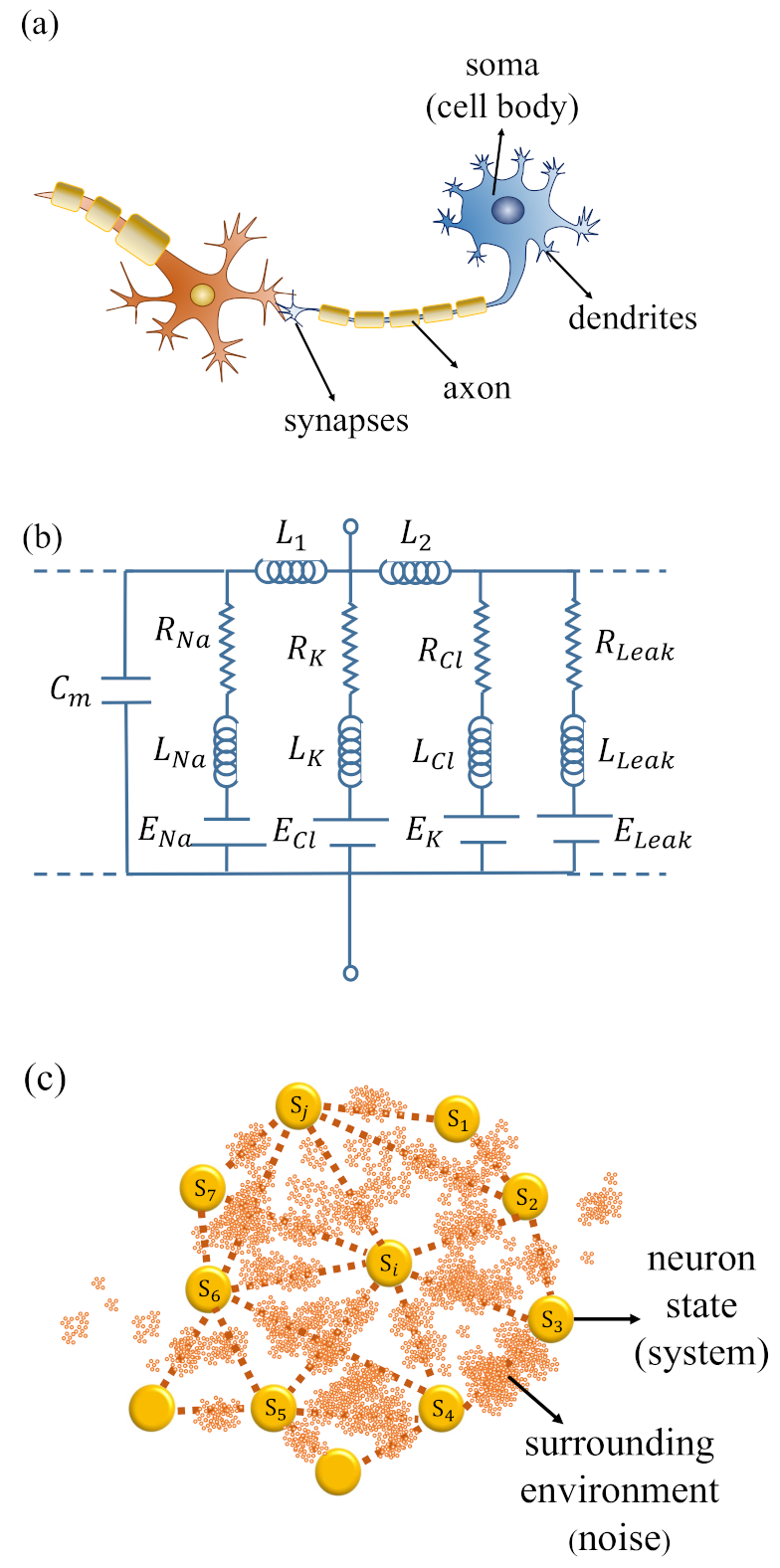
Our motivation is to find the microscopic picture of the random neuron–neuron interaction from the interactions between the neurons and their surroundings (environment). Physically, neuron dynamics are governed by the interaction of neuronal cell body with their surroundings. The surrounding environment consists of all materials surrounding the neuronal cell bodies, including axon, dendrite, synapses and the surrounding glial cells. On the other hand, the neuronal system transmits the electrical signal that one can measure (see Figure 1a). Hodgkin and Huxley used the cable model to explain the electric voltage change of the neuronal membrane through RC circuits. However, the circuit analogy of the neuronal system should contain not only the resistance and capacitors from the fundamental action potential model but also the inductances as observed in some neuronal experiments [30,31]. Consequently, the neuronal system with neural signal transmission among neurons can be taken as more reasonable RLC circuits modified from the action potential model, which is shown in Figure 1b.
In general, any circuit consisting of a complicated combination of RLC circuits corresponds to a collection of coupling harmonic oscillators [32,42]. Explicitly, a RLC circuit is equivalent to a damping LC harmonic oscillator:
which can be obtained from a simple circuit equation , where is the charge in the circuit, is the corresponding circuit current, is the damping rate, is the circuit frequency, and is an external force induced by the external voltage applied to the circuit. Quantum mechanically, a damping LC harmonic oscillator can be obtained microscopically from a principal LC harmonic oscillator linearly coupling to a continuously distribution of many LC harmonic oscillators in the surrounding environment with different frequencies:
as is shown by Feynman and Vernon in their path-integral influence functional theory [32,43], where the first term is the principal LC oscillating Hamiltonian, the second term represents the environment consisting of a continuous distribution of the surrounding LC oscillators. The last term is the coupling of the principal oscillator with the environment oscillators, which results in the damping dynamics.
As a result, we model the neuron cells by a collection of spins, and these neuronal spins can interact with one another through the surrounding materials. The surrounding materials can be modeled by a continuous distribution of harmonic oscillators with all kind of different oscillating frequencies, characterized by Figure 1c, as inspired from the above RLC circuit picture. In quantum mechanics, the collection of the harmonic oscillators with all possible different frequencies can be expressed by the Hamiltonian in the particle number representation:
where the continuous distribution of environmental oscillating modes has been taken and is the density of state of all the oscillating modes in the environment. The operators and are the annihilation and creation operators of the oscillating mode with the corresponding frequency . The interaction between neuron spins and the surrounding materials is provided by the interaction Hamiltonian:
where is the coupling strength between the neuron spin mode and the oscillating mode . The spin raising and lowering operators of each neuron spin are defined as , and N is the total neuron number in the neuronal system. The neuron Hamiltonian of the following:
corresponds to a set of neuron spins in an effective magnetic field g. With the above model description, we obtain our neuronal system described by the following Hamiltonian:
which contains three parts: the Hamiltonian of the neurons, and the Hamiltonian of all oscillating modes from the surroundings, as well as the couplings between them. We will show that it is the coupling between the neurons and their surrounding oscillating modes that is causing the neurons’ connection to one another and resulting in the random neuron–neuron coupling.
3. The Master Equation of the Neuron Dynamics
The neuron dynamics are described by the non-equilibrium evolution of all neuron states in the neuronal system. Neurons can interact with one another through their surrounding environment, as described by the Hamiltonian shown in Equation (9). Quantum mechanically, the total state evolution of neurons plus the environment is determined by the total density matrix , which carries all the state information of the neurons and their surroundings. It is governed by the Liouville–von Neumann equation [44]:
where H is the total Hamiltonian. We focus on the state evolution of the neurons affected by the infinite number of oscillating modes in the environment considered in Equation (9). Thus, we should focus on the time evolution of the reduced density matrix , which is determined by tracing over all the environmental states from the total density matrix: . The reduced density matrix describes the nonequilibrium dynamical evolution of all neuron states in the neuronal system. The equation of motion for the reduced density matrix that determines such evolution is called the master equation, which is derived below.
In the interacting picture of quantum mechanics, the total state of neurons plus their environment in the neuronal system is defined by , where . An expansion solution of Equation (10) in the interacting picture can be written as follows:
where the interacting Hamiltonian is given by , and is the initial state. Suppose that the initial state of the system (neurons) and the environment (surroundings) is a decoupled state , and the environment state is in a thermal equilibrium state, which is , where is the inverse temperature of the environment and is the environmental partition function. Meanwhile, we assume that all the neurons and their surroundings are weakly coupled to one another so that the environmental state almost remains unchanged, namely in Equation (11), which is called as the Born approximation. Since the neurons are weakly coupled to their environment, we can further use the Markov approximation by replacing in the above Born approximation by . After making such Born and Markov approximations, we obtain the trace over all the environmental states. It can be shown that . Then, we obtain the master equation for the reduced density matrix of all the neuron states.
This is known as the Born–Markov master equation in open quantum systems [45].
Now, we apply the above master equation formulation to the Hamiltonian described by Equation (9). For the sake of simplicity, we assume that the coupling strength is a real value, . In the interacting picture, the interaction Hamiltonian is as follows.
After completing the trace over the environmental states in Equation (12) and changing the formulation back into the Schrödinger picture, we have the master equation only with neuron spin degrees of freedom:
which describes the dynamical evolution of all the neuron states in the neuronal system. In Equation (14), the first term at the right hand side is a unitary transformation for the system dynamics according to the renormalized system Hamiltonian , where is induced by the couplings between the neurons and their surroundings:
which characterizes how the disordered neuron–neuron interactions are generated from the coupling between the neurons and their surroundings. The other terms in the master equation describes the dissipation and fluctuations of the neurons induced by the surrounding materials.
The environment-induced neuron–neuron interactions and the dissipation and fluctuation dynamics of neurons are determined by the corresponding time-correlations between the neurons and their surroundings in terms of the time-dependent coefficients in Equation (14):
where and describes the effects of environmentally induced dissipation and fluctuation, and and are the environmentally induced random neuron–neuron couplings. The function is the spectral density of the environment:
and is the density of states of the environmental oscillating spectrum. The spectral density encompasses all the information about the structure of the materials surrounding neurons and the couplings with the neurons. The function is the particle distribution of the environmental oscillating modes and .
The neuronal system contains plenty of dynamical neurons and it is difficult to solve them even numerically. We can lower the calculating cost by summing up all the neuronal operators as a collective neural spin. The collective neural spin is defined by summing up all the neuron spins in each direction :
where . In order to formulate the collective neuron behavior conveniently, we assume that the environment provides the same effect on all the neurons, namely, the coupling strength being independent relative to different neurons, . The spectral density then becomes the following.
As a result, the master Equation (14) is simply reduced to the following form:
where and . The corresponding renormalization and dissipation/fluctuation coefficients in Equation (23) becomes the following.
This is the master equation for the collective neuron states in our physical modeling of neuronal system.
4. Collective Neural Behavior and Neuron Dynamics Analysis
4.1. Equation of Motion for the Collective Neural States
The equations of motion for the collective neural states are obtained through the expectation values of the collective neural spin operators. By taking the expectation value of the collective neural spins with the reduced density matrix, as in the following:
and applying the mean-field approximation, , we obtain a close form of the equation of motion for the collective neural states from Equation (23):
where the coefficients in the above equation of motion are provided by . The coefficients and are related with the neuron–neuron interactions, and and are related to the dissipation and fluctuations. All of them are induced by the couplings between the neurons and with the environment in the neuronal system.
In the following calculation, as an example, we obtain the most common spectral density as follows [43]:
where is a dimensionless coupling constant between the system and the environment, and is a cut-off frequency. The value of s can be , and , corresponding to the spectrum of the environment Ohmic, sub-Ohmic and super-Ohmic spectrum, respectively. Here, we consider the Ohmic spectrum, . With such detailed structure for the neuron environment, we can study the collective neuron behavior induced by the environment effects.
4.2. The Dynamics of Collective Neural States
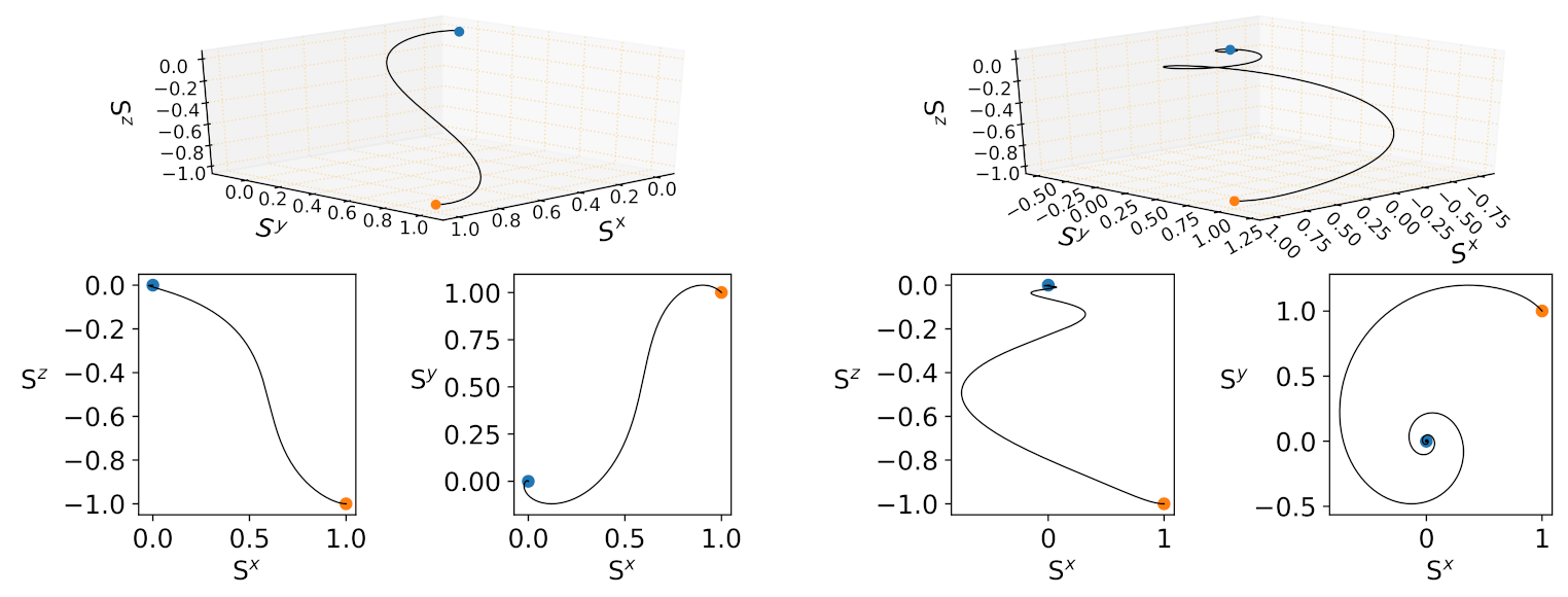
With the equation of motion, Equations (29)–(31), obtained from the master equation, we want to explore how the collective neural states evolve in time under coupling with their surroundings. We start from the collective neural states and study the time evolution of the collective state under different coupling constants. The results are presented in Figure 2, with the coupling strength being and . As one can observe, the system always flows to the (0, 0, 0) state, which corresponds to the depolarized state. The differences are manifested in the trajectories of the collective neural states in the phase space. The larger the coupling constant, the sooner the collective neural state is depolarized.
In reality, the neural signal transmissions through the external pulses stimulate the neurons. In the following, we want to explore how the collective neural states evolve in time when exerting an external pulse to the system by replacing the constant coupling strength with a rectangular pulse. In order to investigate the collective neural dynamics, we consider first the simple case of the nervous system at zero temperature and then move to the more realistic case of the neuron system at room temperature.
4.2.1. Collective Neural Dynamics at Zero Temperature
In order to consider an external pulse acting on the neuronal system, we modify the coupling as a time dependent parameter.
Meanwhile, at zero temperature, the dissipation and fluctuation coefficients in the master equation are reduced to the following:
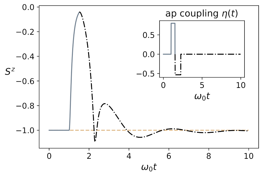
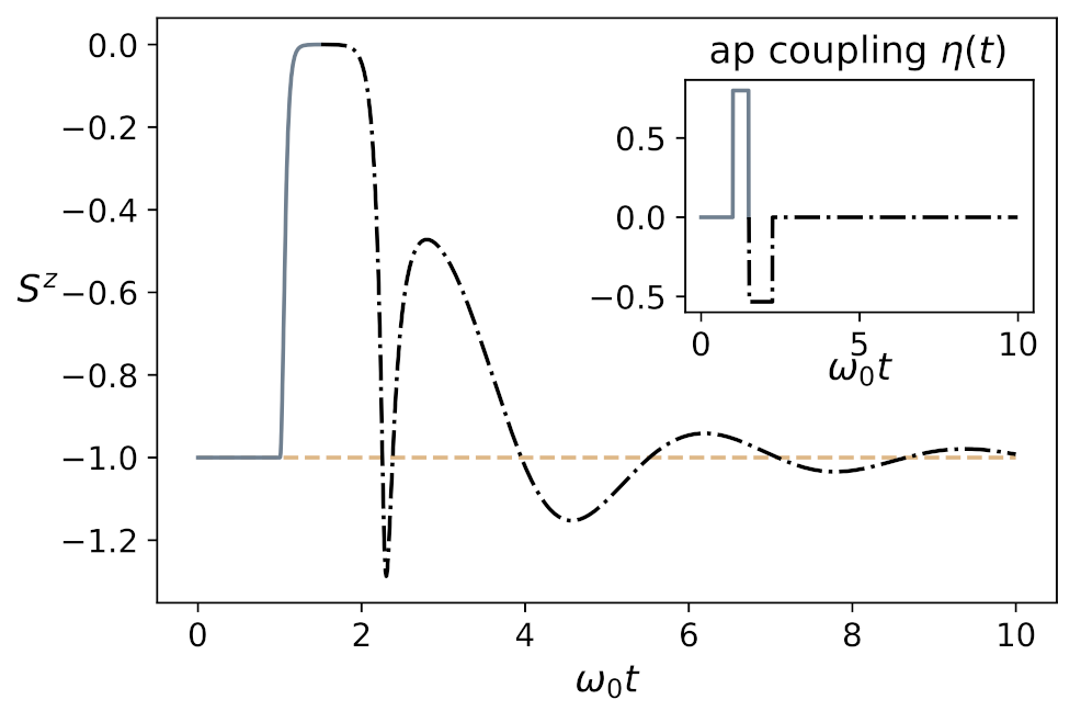
and follows. Figure 3 shows the dynamics of the collective neural state after stimulation. We apply a simple square pulse with amplitude up to for depolarizing the neural state (see the inset in Figure 3). The gray lines in Figure 3 represents time from 0 to 1.5 (), and the black-dashed line represents time from 1.5 to 10 (), where the duration time is scaled by the system frequency defined as Hz. Initially, the collective neural state is at polarized state (, , ) = (0, 0, −1). At the time from 0 to 1 (), no environmental noise exists, and the neuron system is in the rest state. At time from 1 to 1.5 (), we exert a pulse with amplitude 0.8, and the system reaches the depolarized state (, , ) ≈ (0, 0, 0). In the retrieving process, we extended the time duration to one and a half and made comparisons with the storing process and changed the coupling to 1.5 times less at time 1.5 to 2.25 (). The neural state then proceeds backward and experiences the repolarized process. Finally, during the time from 2.25 to 10 (), the system gradually returns to the initial rest state.
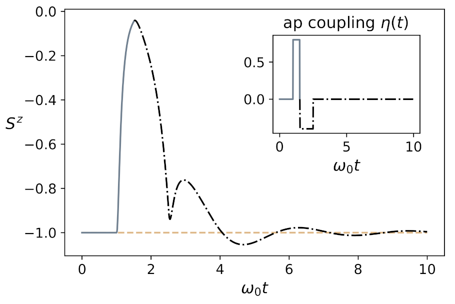
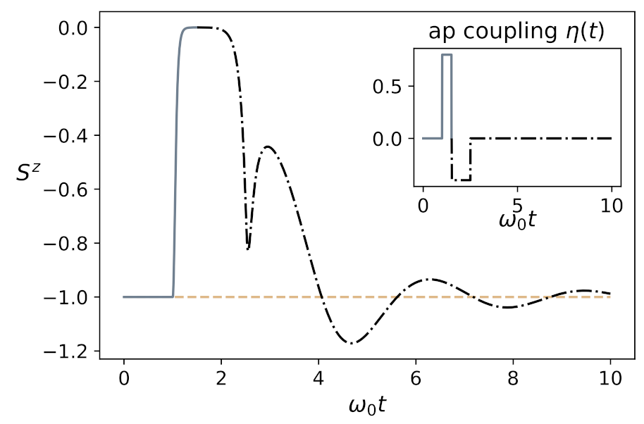
In Figure 4, we consider the stimulation when it doubles in time and becomes half in terms of quantity (refer to the inset of Figure 4). The result shows that the collective neural state can still repolarized to the original rest state. The similar action potential behavior was demonstrated from the collective neural state. This phenomenon shows that the stimulation of the neuronal system activates almost half of the neurons so that the collective neural state can reach the depolarized state “”. This is the “depolarization” mechanism of the neuron states via the environmental stimulation in our neuronal model.
4.2.2. Collective Neural Dynamics at Room Temperature
However, the zero temperature condition is an ideal case. The biosystem survives within room temperature. The increase in temperature will provide more noise from the environment. If we consider the environment at room temperature, all the dissipation and fluctuation coefficients of Equations (24)–(27) remain. At room temperature ( K), the particle distribution in the environment can take on the classical Boltzmann distribution . The state evolution under the room-temperature-environmental effect is shown in Figure 5. In this case, we find that it takes longer time for the state returning back to the initial rest state through the depolarization and repolarization processes due to the environment fluctuation on the collective neural state. This result also shows that no more than a half of the neurons are fired, and thus the maximum amplitude of the collective neural state is a little bit less than 0, but the temperature effect renders the firing states closer to the depolarized state. Furthermore, the condition of the same area also holds with the non-zero-temperature. The result is shown in Figure 6 for the same pulse profile in Figure 4.
5. Conclusions
In conclusion, we built a neuronal model as an open quantum system in order to understand the randomly coupled neuron–neuron interaction through their coupling with the neural environment. We used the master equation approach to studied the collective behavior of neurons incorporating the pulse stimulation in order to demonstrate the action potential. We explored the neuron dynamics at zero temperature and also at room temperature and found that, in both cases, the collective neural states evolved from polarized states (rest states) to the depolarized states and, finally, back to the initial polarized states under a simplified external pulse driving the neuronal system. Such results show that this simple neuronal model can not only catch the expected neuron dynamics but also provide an alternative mechanism in explaining how neurons couple or connect to one another through the complicated neuronal surrounding oscillating modes. As the result also shows, neuron–neuron connections through their surroundings are mainly determined by the spectral density of the neural surrounding environment, which characterizes the detailed energy spectrum structure of the neuronal environment. In this work, we only used the simple Ohmic spectral density as an example to simulate the collective neuron dynamics. The more realistic description of neuron dynamics relies on the spectral density that should be obtained from the spectral measurement of the neuron surroundings. Furthermore, a more complete description of the underlying neuron dynamics should be given by the neuron firing distribution in the neuronal system, which is depicted by the reduced density matrix of the master equation and can be obtained by solving the master equation directly. These remain open for the further investigations.
Author Contributions
Y.-J.S. and W.-M.Z. conceived and worked together to produce this manuscript; W.-M.Z. proposed the ideas and supervised the project; Y.-J.S. performed all calculations; Y.-J.S. and W.-M.Z. analyzed and interpreted the results and completed the writing of the manuscript. All authors have read and agreed to the published version of the manuscript.
Funding
This work is supported by the Ministry of Science and Technology of Taiwan under Contract: MOST-108-2112-M-006-009-MY3.
Institutional Review Board Statement
Not applicable.
Informed Consent Statement
Not applicable.
Data Availability Statement
Not applicable.
Acknowledgments
The authors would like to thank M.S. Yang, H.L. Lai and W.M. Huang for their fruitful discussions.
Conflicts of Interest
The authors declare no conflict of interest.
References
- Tortora, G.J.; Derrickson, B.H. Principles of Anatomy and Physiology; John Wiley & Sons: Hoboken, NJ, USA, 2018. [Google Scholar]
- LeCun, Y.; Bengio, Y.; Hinton, G. Deep learning. Nature 2015, 521, 436–444. [Google Scholar] [CrossRef] [PubMed]
- Voulodimos, A.; Doulamis, N.; Doulamis, A.; Protopapadakis, E. Deep learning for computer vision: A brief review. Comput. Intell. Neurosci. 2018, 2018. [Google Scholar] [CrossRef] [PubMed]
- Nassif, A.B.; Shahin, I.; Attili, I.; Azzeh, M.; Shaalan, K. Speech recognition using deep neural networks: A systematic review. IEEE Access 2019, 7, 19143–19165. [Google Scholar] [CrossRef]
- Evgeniou, T.; Pontil, M. Regularized Multi–Task Learning. In Proceedings of the Tenth ACM SIGKDD International Conference on Knowledge Discovery and Data Mining, KDD ’04, Seattle, WA, USA, 22–25 August 2004; Association for Computing Machinery: New York, NY, USA, 2004; pp. 109–117. [Google Scholar] [CrossRef]
- Xiao, Y.; Codevilla, F.; Gurram, A.; Urfalioglu, O.; López, A.M. Multimodal end-to-end autonomous driving. IEEE Trans. Intell. Transp. Syst. 2020, 1–11. [Google Scholar] [CrossRef]
- Hassabis, D.; Kumaran, D.; Summerfield, C.; Botvinick, M. Neuroscience-inspired artificial intelligence. Neuron 2017, 95, 245–258. [Google Scholar] [CrossRef] [PubMed] [Green Version]
- Turing, A.M. On computable numbers, with an application to the Entscheidungsproblem. Proc. Lond. Math. Soc. 1937, 2, 230–265. [Google Scholar] [CrossRef]
- Turing, A.M. Computing machinery and intelligence. In Parsing the Turing Test; Springer: Dordrecht, The Netherlands, 2009; pp. 23–65. [Google Scholar] [CrossRef]
- McCulloch, W.S.; Pitts, W. A logical calculus of the ideas immanent in nervous activity. Bull. Math. Biophys. 1943, 5, 115–133. [Google Scholar] [CrossRef]
- Hodgkin, A.L.; Huxley, A.F. A quantitative description of membrane current and its application to conduction and excitation in nerve. J. Physiol. 1952, 117, 500–544. [Google Scholar] [CrossRef]
- Cole, K.S.; Curtis, H.J. Electric impedance of the squid giant axon during activity. J. Gen. Physiol. 1939, 22, 649–670. [Google Scholar] [CrossRef] [PubMed] [Green Version]
- Hodgkin, A.L.; Katz, B. The effect of sodium ions on the electrical activity of the giant axon of the squid. J. Physiol. 1949, 108, 37–77. [Google Scholar] [CrossRef]
- Keynes, R. The ionic movements during nervous activity. J. Physiol. 1951, 114, 119–150. [Google Scholar] [CrossRef] [Green Version]
- Hodgkin, A.L. The Conduction of the Nervous Impulse; Sherrington Lectures; Liverpool University Press: Liverpool, UK, 1971. [Google Scholar]
- Bean, B.P. The action potential in mammalian central neurons. Nat. Rev. Neurosci. 2007, 8, 451–465. [Google Scholar] [CrossRef]
- Hebb, D.O. The organization of behavior: A neuropsychological theory. Wiley Book Clin. Psychol. 1949, 62, 78. [Google Scholar]
- Hopfield, J.J. Neural networks and physical systems with emergent collective computational abilities. Proc. Natl. Acad. Sci. USA 1982, 79, 2554–2558. [Google Scholar] [CrossRef] [PubMed] [Green Version]
- Sofroniew, M.V.; Vinters, H.V. Astrocytes: Biology and pathology. Acta Neuropathol. 2010, 119, 7–35. [Google Scholar] [CrossRef] [Green Version]
- Kaufmann, K.; Hanke, W.; Corcia, A. Ion Channel Fluctuations in Pure Lipid Bilayer Membranes: Control by Voltage; Caruaru, Brazil; 1989. Available online: http://membranes.nbi.dk/Kaufmann/pdf/Kaufmannbook3ed.pdf (accessed on 29 May 2021).
- Pollack, G.H. Cells, Gels and the Engines of Life: A New, Unifying Approach to Cell Function; Ebner & Sons: Seattle, WA, USA, 2001. [Google Scholar]
- Ivanova, V.; Makarov, I.; Schäffer, T.; Heimburg, T. Analyzing heat capacity profiles of peptide-containing membranes: Cluster formation of gramicidin A. Biophys. J. 2003, 84, 2427–2439. [Google Scholar] [CrossRef] [Green Version]
- Heimburg, T.; Jackson, A.D. On soliton propagation in biomembranes and nerves. Proc. Natl. Acad. Sci. USA 2005, 102, 9790–9795. [Google Scholar] [CrossRef] [Green Version]
- Arraut, I. Black-hole evaporation from the perspective of neural networks. EPL 2018, 124, 50002. [Google Scholar] [CrossRef] [Green Version]
- Rose, D.C.; Macieszczak, K.; Lesanovsky, I.; Garrahan, J.P. Metastability in an open quantum Ising model. Phys. Rev. E 2016, 94, 052132. [Google Scholar] [CrossRef] [Green Version]
- Rotondo, P.; Marcuzzi, M.; Garrahan, J.P.; Lesanovsky, I.; Müller, M. Open quantum generalisation of Hopfield neural networks. J. Phys. A Math. Theor. 2018, 51, 115301. [Google Scholar] [CrossRef] [Green Version]
- Damanet, F.; Daley, A.J.; Keeling, J. Atom-only descriptions of the driven-dissipative Dicke model. Phys. Rev. A 2019, 99, 033845. [Google Scholar] [CrossRef] [Green Version]
- Glauber, R.J. Time-dependent statistics of the Ising model. J. Math. Phys. 1963, 4, 294–307. [Google Scholar] [CrossRef]
- Peretto, P. Collective properties of neural networks: A statistical physics approach. Biol. Cybern. 1984, 50, 51–62. [Google Scholar] [CrossRef] [PubMed]
- Cole, K.S.; Baker, R.F. Longitudinal impedance of the squid giant axon. J. Gen. Physiol. 1941, 24, 771–788. [Google Scholar] [CrossRef] [PubMed]
- Wang, H.; Wang, J.; Thow, X.Y.; Lee, S.; Peh, W.Y.X.; Ng, K.A.; He, T.; Thakor, N.V.; Chen, C.H.; Lee, C. Inductance in neural systems. bioRxiv 2018, 343905. [Google Scholar] [CrossRef] [Green Version]
- Feynman, R.P.; Vernon, F.L., Jr. The theory of a general quantum system interacting with a linear dissipative system. Ann. Phys. 2000, 281, 547–607. [Google Scholar] [CrossRef] [Green Version]
- Rosenblatt, F. Principles of Neurodynamics. Perceptrons and the Theory of Brain Mechanisms; Technical Report; Cornell Aeronautical Lab Inc.: Buffalo, NY, USA, 1961. [Google Scholar] [CrossRef]
- Cooper, L.N.; Liberman, F.; Oja, E. A theory for the acquisition and loss of neuron specificity in visual cortex. Biol. Cybern. 1979, 33, 9–28. [Google Scholar] [CrossRef]
- Longuet-Higgins, H.C. The non-local storage of temporal information. Proc. R. Soc. Lond. Ser. B Biol. Sci. 1968, 171, 327–334. [Google Scholar] [CrossRef]
- Longuet-Higgins, H.C. Holographic model of temporal recall. Nature 1968, 217, 104. [Google Scholar] [CrossRef]
- Kohonen, T. Associative Memory: A System-Theoretical Approach; Springer Science & Business Media: Berlin/Heidelberg, Germany, 2012; Volume 17. [Google Scholar]
- Amari, S.I. Neural theory of association and concept-formation. Biol. Cybern. 1977, 26, 175–185. [Google Scholar] [CrossRef]
- Amari, S.I.; Takeuchi, A. Mathematical theory on formation of category detecting nerve cells. Biol. Cybern. 1978, 29, 127–136. [Google Scholar] [CrossRef] [PubMed]
- Little, W.A. The existence of persistent states in the brain. Math. Biosci. 1974, 19, 101–120. [Google Scholar] [CrossRef]
- Amit, D.J.; Gutfreund, H.; Sompolinsky, H. Spin-glass models of neural networks. Phys. Rev. A 1985, 32, 1007. [Google Scholar] [CrossRef]
- Weiss, U. Quantum Dissipative Systems; World Scientific: Singapore, 2012; Volume 13. [Google Scholar] [CrossRef]
- Leggett, A.J.; Chakravarty, S.; Dorsey, A.T.; Fisher, M.P.; Garg, A.; Zwerger, W. Dynamics of the dissipative two-state system. Rev. Mod. Phys. 1987, 59, 1. [Google Scholar] [CrossRef]
- Von Neumann, J. Mathematical Foundations of Quantum Mechanics: New Edition; Princeton University Press: Princeton, NJ, USA, 2018. [Google Scholar]
- Breuer, H.P.; Petruccione, F. The Theory of Open Quantum Systems; Oxford University Press on Demand: Oxford, UK, 2002. [Google Scholar]
Figure 1.
(a) The structure of realistic neuron cells. (b) An extended action potential RLC circuit for mimicking neural signal transmissions in neuronal systems. (c) Our modeling of the neuronal system as a collection of neuronal cell bodies interacting with one another through their surrounding environmental materials.

Figure 2.
Collective neural state evolution of the neurons coupled to the environment effect with different couplings. The couplings are (a) and (b) . The temperature is taken in K (room temperature), where determines the system frequency Hz.
Figure 2.
Collective neural state evolution of the neurons coupled to the environment effect with different couplings. The couplings are (a) and (b) . The temperature is taken in K (room temperature), where determines the system frequency Hz.

Figure 3.
State evolution of the collective neurons under stimulation (refer to the inset). The coupling during the storing process is set as 0.8 at the time from 1 to 1.5 (), and it is set as −0.53 at the time from 1.5 to 2.25 () during the retrieving process. The system frequency is defined as g.
Figure 3.
State evolution of the collective neurons under stimulation (refer to the inset). The coupling during the storing process is set as 0.8 at the time from 1 to 1.5 (), and it is set as −0.53 at the time from 1.5 to 2.25 () during the retrieving process. The system frequency is defined as g.

Figure 4.
State evolution of the collective neurons with the positive/negative coupling in the same area relative to the time axis. The negative coupling becomes twice in terms of time and half in terms of quantity. The coupling during the storing process is set as 0.8 at the time from 1.00 to 1.5 (), and it is set as −0.4 at the time from 1.5 to 2.5 () during the retrieving process. The system frequency is defined as g.

Figure 5.
State evolution of the collective neural state for the system considering the environment in finite temperature ( K). The coupling during the storing process is set as 0.80 at the time from 1.00 to 1.50 () and, during the retrieving process, it is set as −0.53 at the time from 1.50 to 2.25 ().


Publisher’s Note: MDPI stays neutral with regard to jurisdictional claims in published maps and institutional affiliations. |
© 2021 by the authors. Licensee MDPI, Basel, Switzerland. This article is an open access article distributed under the terms and conditions of the Creative Commons Attribution (CC BY) license (https://creativecommons.org/licenses/by/4.0/).
Share and Cite
MDPI and ACS Style
Sun, Y.-J.; Zhang, W.-M. Modeling Neuronal Systems as an Open Quantum System. Symmetry 2021, 13, 1603. https://doi.org/10.3390/sym13091603
AMA Style
Sun Y-J, Zhang W-M. Modeling Neuronal Systems as an Open Quantum System. Symmetry. 2021; 13(9):1603. https://doi.org/10.3390/sym13091603
Chicago/Turabian StyleSun, Yu-Juan, and Wei-Min Zhang. 2021. "Modeling Neuronal Systems as an Open Quantum System" Symmetry 13, no. 9: 1603. https://doi.org/10.3390/sym13091603
Note that from the first issue of 2016, this journal uses article numbers instead of page numbers. See further details here.