
Electroweak Effects in e+e−→ZH Process
by
 , , , and
Andrej Arbuzov
1,2,† ,
,
Serge Bondarenko
1,*,† ,
,
Lidia Kalinovskaya
3,†,
Renat Sadykov
3,† and
Vitaly Yermolchyk
3,4,† 1
Bogoliubov Laboratory of Theoretical Physics, JINR, Joliot-Curie str. 6, 141980 Dubna, Russia
2
Chair of Fundamental Problems of Microworld Physics, Dubna State University, Universitetskaya str. 19, 141982 Dubna, Russia
3
Dzhelepov Laboratory of Nuclear Problems, JINR, Joliot-Curie str. 6, 141980 Dubna, Russia
4
Institute for Nuclear Problems, Belarusian State University, 220006 Minsk, Belarus
*
Author to whom correspondence should be addressed.
†
These authors contributed equally to this work.
Symmetry 2021, 13(7), 1256; https://doi.org/10.3390/sym13071256
Submission received: 23 May 2021
/
Revised: 7 June 2021
/
Accepted: 9 June 2021
/
Published: 13 July 2021
(This article belongs to the Special Issue Symmetry in Particle Physics II)
Abstract
:Electroweak radiative corrections to the cross-section of the process are considered. The complete one-loop electroweak radiative corrections are evaluated with the help of the SANC system. Higher-order contributions of the initial-state radiation are computed in the QED structure function formalism. Numerical results are produced by a new version of the ReneSANCe event generator and MCSANCee integrator for the conditions of future electron-positron colliders. The resulting theoretical uncertainty in the description of this process is estimated.
Keywords:
high-energy physics; electron-positron annihilation; forward-backward asymmetry; left-right asymmetryPACS:
12.15.-y; 12.15.Lk; 13.66.Jn1. Introduction
The Standard Model (SM) is extremely successful in describing various phenomena in particle physics. Despite this fact, there are many reasons to consider the SM as an effective model, i.e., a low-energy approximation of a more general theory. Looking for the limits of the SM applicability domain is one of the most valuable problems in modern fundamental physics. On the other hand, a deep investigation of the SM properties at the quantum level is still an important task since this model is relevant for many applications in high-energy physics as well as astrophysics and cosmology. In this context, exploring the Higgs boson sector of the SM is crucial for checking the mechanism of spontaneous symmetry breaking and finalizing the verification of the model within the energy range achieved at modern accelerators.
To perform an in-depth verification of the Standard Model and define the energy region of its applicability, we certainly need a new high-energy accelerator. An electron-positron collider with energies of a few hundred GeV looks now to be the best option. Several projects of this kind of machine are being under consideration, e.g., ILC [1], CLIC [2], CEPC [3], and FCC-ee [4]. Programs of all these colliders, except CLIC, necessarily include the option to run as Higgs factories with center-of-mass system (c.m.s.) energies of about 240 GeV. At this energy, the maximal count rate of events of the processes can be reached. Collecting several million such events will substantially increase the precision of the Higgs boson mass and the determination of the partial decay widths [5,6].
The expected high statistics of events with Higgs bosons challenges the theory to provide very accurate SM predictions for the corresponding processes with uncertainty at the permille level. So, we need to take into account radiative corrections in the first and higher orders of perturbation theory (Non-perturbative effects due to strong interactions are also relevant in running EW couplings and in producing extra meson pairs). The status of high-precision calculations for FCC-ee (and other future colliders in general) is described in [7].
In this work, we analyze QED and electroweak (EW) radiative corrections to the higgsstrahlung process
This process is the most promising one in studying the Higgs boson properties. So, the accuracy of its theoretical description should be higher than the experimental precision so that the combined uncertainty in the results of data analysis would not be spoiled by the theory. The uncertainty estimate should be as complete as possible.
In this paper, we evaluate the complete one-loop corrections supplemented by higher-order (HO) QED contributions in the leading logarithmic approximation (LLA) [8]. Our aim is to analyze the size of different HO contributions, estimate the resulting theoretical uncertainty, and verify the necessity to include other HO corrections. Please note that in this work we do not consider decays of Z and H, which are left for further study.
The complete one-loop electroweak radiative corrections to the process under consideration were computed with the help of the SANC computer system and reported in [9]. Here we will concentrate on the analysis of the HO QED effects. Recently, effects due to higher-order initial-state radiation (ISR) of photons in the process were considered in [10]. The channel with Z and H bosons in this process was included. It was claimed that the third order leading logarithmic contribution is numerically important and should be included. Here we study QED ISR corrections in more detail with taking into account radiation of light pairs, photonic leading logarithmic contributions up to the fourth order, and the complete one-loop (electro)weak effects.
Two-loop QED corrections due to the initial-state radiation for a general process of high-energy electron-positron annihilation through a virtual photon or Z boson were calculated in [11] and recently corrected in [12]. Higher-order QED ISR contributions in the leading and next-to-leading logarithmic approximations up to the order were given in [13]. These results are performed in an inclusive set-up where only the distribution in the invariant mass of the final state particles is available. So, they provide a benchmark for comparisons while for practical applications one needs a Monte Carlo simulation with complete kinematics.
The paper is organized as follows. In Section 2, we outline the contributions due to the higher-order QED initial-state radiation order by order. In Section 3, we present the numerical results for the cross-section of associated production in the energy region GeV. Our conclusions are given in Section 4.
2. ISR Corrections in LLA Approximation
2.1. General Notes
Let us consider ISR corrections to processes of high-energy electron-positron annihilation within the LLA. They can be evaluated with the help of the QED structure function formalism [8]. For ISR corrections in the annihilation channel the large logarithm is where the total c.m.s. energy is chosen as factorization scale.
The master formula for a general annihilation cross-section with ISR QED corrections in the leading logarithmic approximation has the same structure as the one for the Drell–Yan process, it reads
where is the Born-level cross-section of the annihilation process with reduced energies of the incoming particles. Here we do not take into account “photon induced” contributions, since the corresponding kernel cross-sections and are very much suppressed by extra powers of the fine structure constant .
The electron structure functions, or better to say electron parton density functions, describe the density of probability to find an electron with an energy fraction x in the initial electron beam [8,14,15]. Please note that the electron parton distribution functions in QED are completely analogous to proton PDF in QCD except the possibility to compute them in the QED case.
In the LLA approximation we can separate the pure photonic corrections (marked “”) and the remaining ones which include the pure pair and mixed photon-pair effects (marked as “pair”) as follows:
Pair corrections can be separated into singlet and non-singlet ones . We take into account both by default.
Non-singlet splitting functions can be represented in the form
with being the soft-hard separator. For example,
Higher-order non-singlet pure photonic splitting functions are obtained by iterations of convolution
see the details in Ref. [15].
The singlet splitting functions and are not singular at , so they do not contain parts. Explicit expressions for all relevant splitting functions are given in Refs. [15,16].
The Born-level partonic cross-section is known in the partonic c.m.s. as , where . The transition from the partonic c.m.s. into the laboratory reference frame is required if .
Let us classify contributions with different kinematics:
- I.
- The Born kinematics: additional contributions to Born+Soft+Virt.
- II.
- One hard photon collinear to the first initial particle with possible soft and/or virtual (Soft+Virt) corrections to the second one. Hereafter “One hard photon” means “at least one hard photon in the same direction”.
- III.
- Soft+Virt to the first initial particle and one hard photon along the second initial particle.
- IV.
- One hard photon along the first initial particle and one along the second one.
Separation of hard and soft photon emission is provided by the dimensionless parameter with typical values , . Under all integrals relevant (process dependent) cuts on the lower values of and variables should be applied.
Application of representation (6) in structure functions (3) and their substitution into the master Equation (2) gives the corrected cross-section in the LLA approximation. We expand the result in and look at the second, third, and fourth order contributions.
A few general comments are in order:
- •
- The first lower index below denotes the order in .
- •
- Factorials and coefficients are given explicitly in order to see their structure.
- •
- For pure photonic LLA corrections the traditional shift is carried out, it takes into account part of the next-to-leading (NLO) corrections. However, for pair corrections such a shift is not well justified, and we keep the large log unchanged.
2.2. First Order LLA Contributions
There are only photonic corrections in . Below we list the contributions of different kinematics.
I. Born kinematics
II. Emission only along the first particle
III. Emission only along the second particle
IV. Emission along both initial particles
2.3. Second Order LLA Contributions
I. Born kinematics
II. Emission only along the first particle
III. Emission only along the second particle
IV. Emission along both initial particles
2.4. Third Order LLA Contributions
I. Born kinematics
II. Emission only along the first particle
III. Emission only along the second particle
IV. Emission along both initial particles
2.5. Fourth Order LLA Contributions
Here we list only pure photonic contributions due to the smallness of pair corrections in the fourth order.
I. Born kinematics
II. Emission only along the first particle
III. Emission only along the second particle
IV. Emission along both initial particles
2.6. LLA Contributions for Helicity States
However, singlet contributions of pair corrections can be separated for different helicities:
Since QED preserves parity,
2.7. Scheme with Exponentiation
In the master Equation (2), the electron structure functions can be taken in the exponentiated form [18,19]. That would mean continuous integration over without the auxiliary parameter . The result of [19] contains only the pure photonic corrections and corresponds to the inclusion of exact leading logs up to the order together with approximate (incomplete) HO LLA effects. Please note that the HO exponentiated effects become exact (in LLA) in the soft photon limit.
- •
- •
- The exponentiated structure functions include the LLA part of one-loop QED radiative corrections. To avoid double counting with complete one-loop corrections, we need to subtract the first order leading logarithmic terms from one-loop corrections. So, the final result reads
The “Soft+Virt” part has the Born-like kinematics:
where is the dimensionless soft-hard separator from the original complete one-loop formulae implemented in the Monte Carlo generator.
The “Hard LLA” term is rewritten to match “Hard” kinematics:
3. Numerical Results
In this section, we show numerical results for one-loop EW and HO QED radiative corrections to the process. The input parameters can be found in [9]. The results are obtained without any angular cuts. The relative correction (in %) is defined as
To illustrate the trends of the ISR contribution behavior, we present separate distributions for each , term and their sum as a function of the c.m.s. energy.
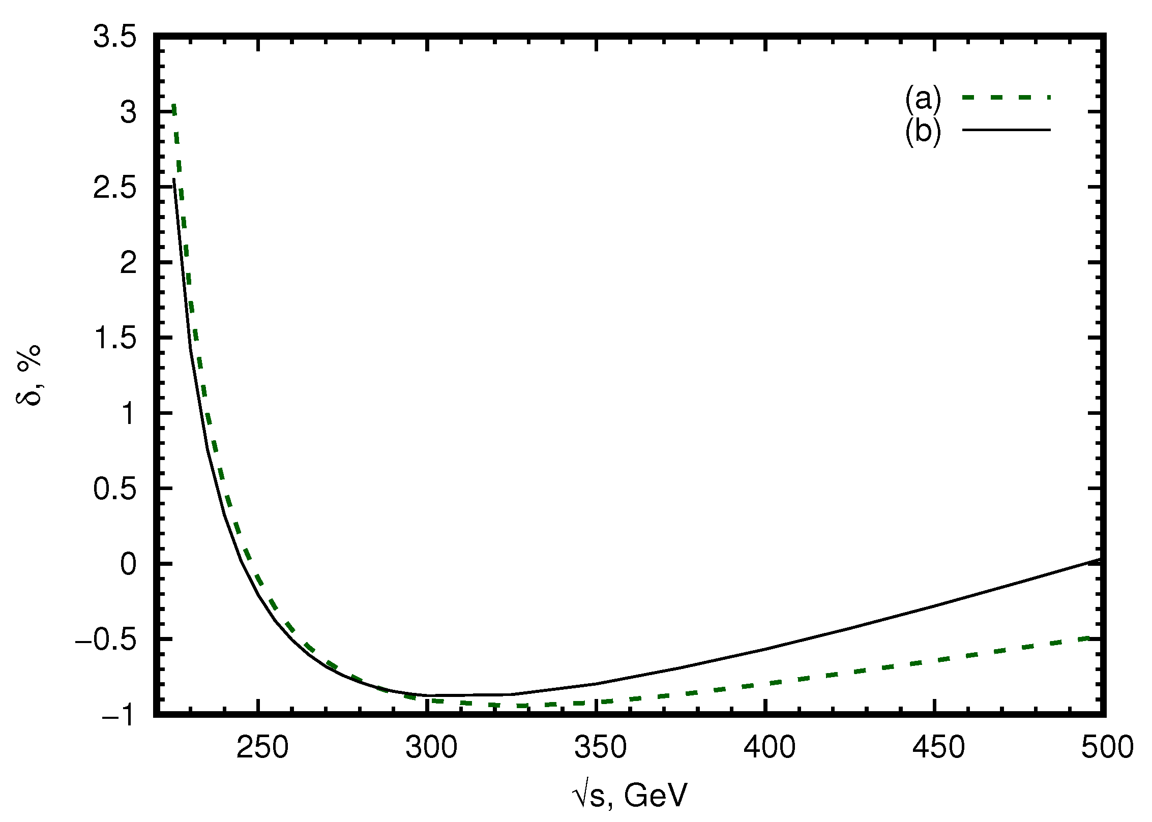
Figure 1 shows the values of the dominant contribution and the sum of all considered orders of the ISR terms vs. c.m.s. energy. The dominant contribution is about 3% at the c.m.s. energy GeV, then it crosses the zero line approximately at GeV, reaches the minimum value about at 325 GeV and goes to at GeV. The sum is mainly determined by the term in the region of c.m.s energies GeV and becomes close to zero at GeV.
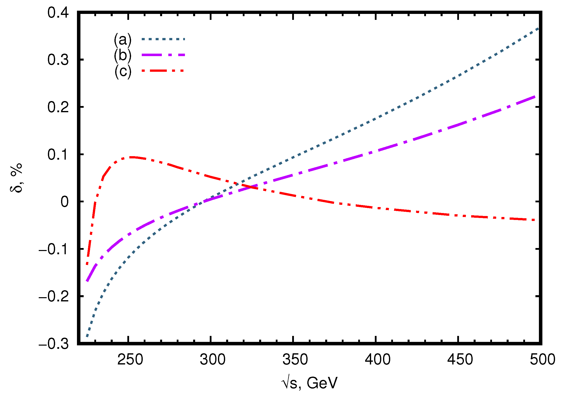
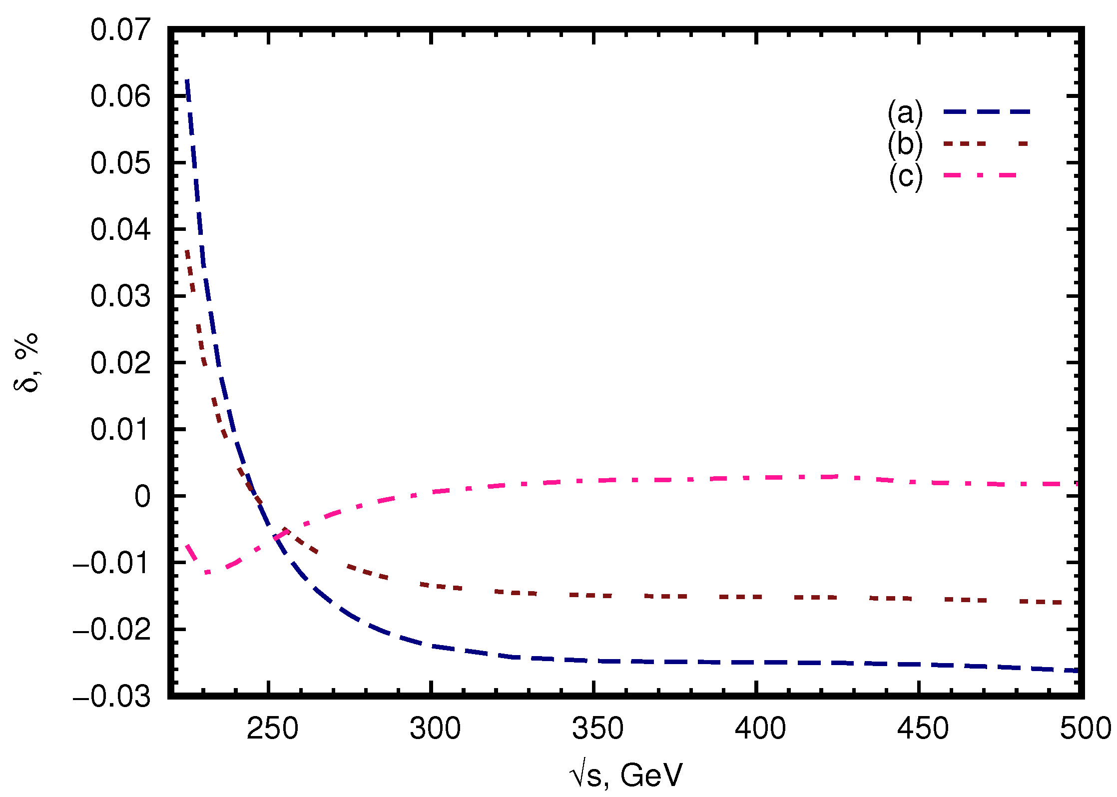
Figure 2 demonstrates the values of the contribution of relative correction (in %): (a) , (b) , (c) vs. c.m.s. energy. Figure 3 shows the values of the contribution of relative correction (in %): (a) , (b) , (c) vs. c.m.s. energy. The second order contributions due to light pair emission are smaller than second order photonic corrections. The suppression of pair corrections with respect to photonic ones in the same order is typical in annihilation processes at LEP energies [21]. However, there is a kinematical region where they are comparable. See, for example regions near 240 GeV (Table 1) and 250 GeV (Table 2) and also near 500 GeV. The third (fourth) order photonic corrections are approximately 10 (100) times smaller than .
One can see that in the threshold energy region there are several competing contributions with different behavior. This confirms the necessity to take into account HO QED ISR contributions in the studies of the higgsstrahlung process at future colliders. The pair and photon contributions should be taken into account for the accuracy goal (see Figure 3).
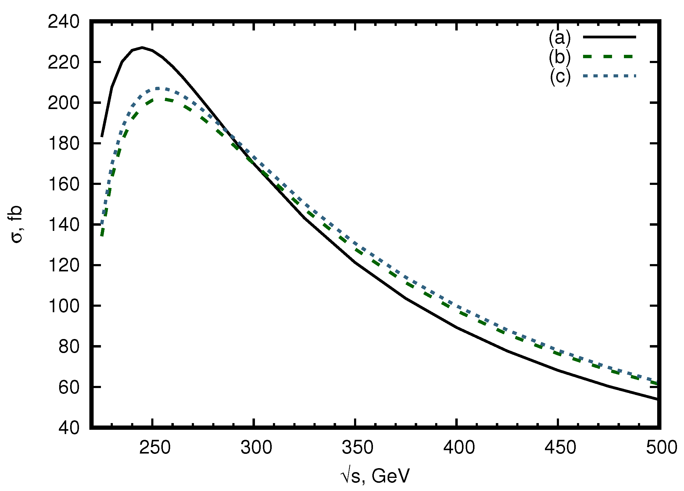
Figure 4 illustrates the behavior of the cross-sections with respect to the c.m.s. energy. It is seen that at the peak in the threshold region, the one-loop QED corrections change not only the height of the peak but also its shape and position.
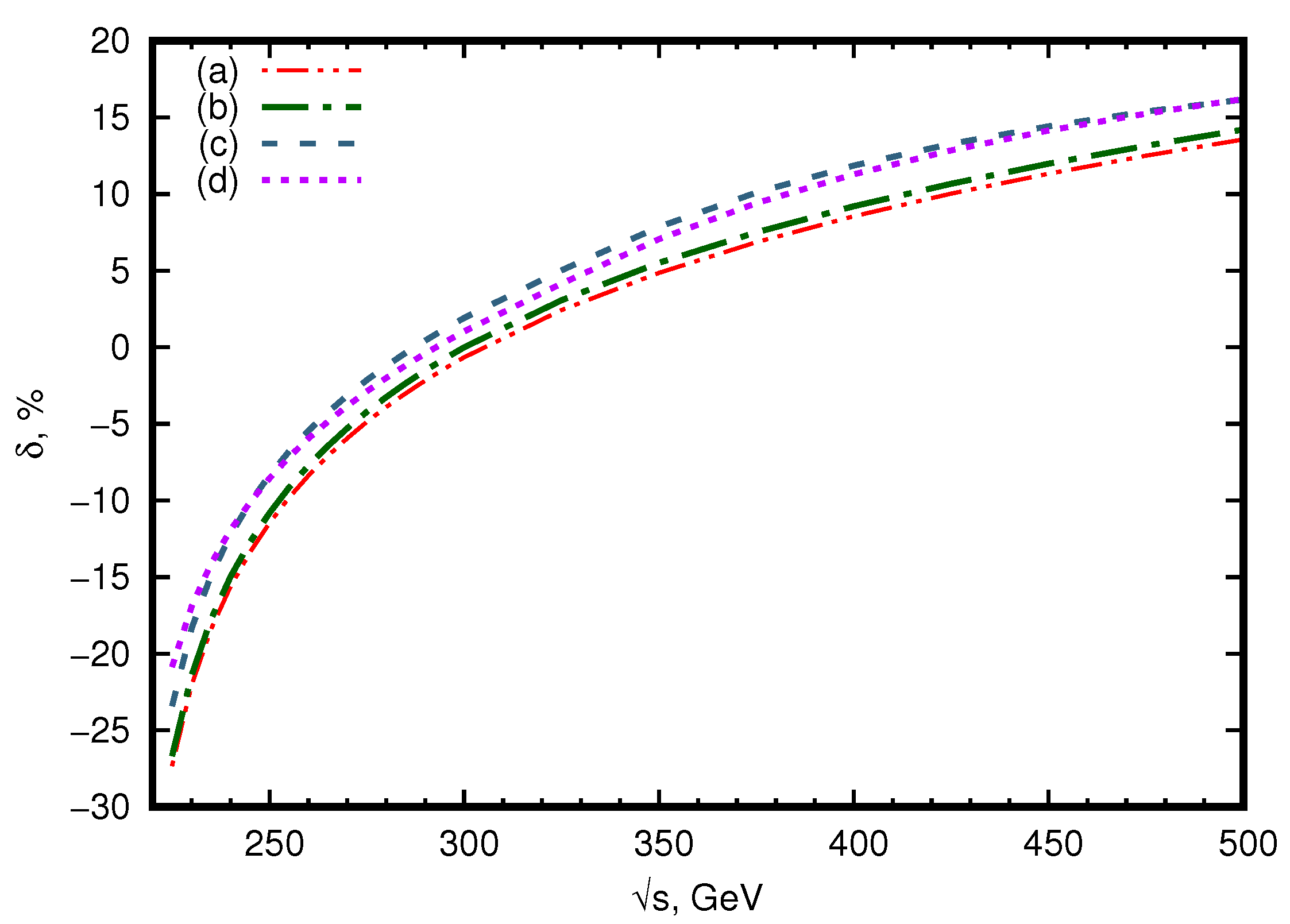
Figure 5 complements Figure 4. It shows the size of the relative RC in different approximations. One can see the difference between the first order term (a) and exact QED corrections (b) and that the HO ISR LLA contributions provide a small but visible shift (the difference between lines (c) and (d)) from the complete one-loop EW correction. Moreover, this shift changes its sign.
In Table 1 and Table 2 we show the ISR corrections of different order of = 2–4 in the LLA approximation for the c.m.s. energies GeV and 250 GeV in the EW scheme. We provide numbers in two points because these energies are particular for the process under consideration. Specifically, the Born-level cross-section has a peak at ∼240 GeV while the present plans of future colliders envisage operation at 250 GeV where the counting rate of the signal is higher [3,4].
It is seen in Table 1 and Table 2 that the corrections for the sum of all considered orders of the ISR terms are about 0.322% for the c.m.s. energy GeV and about −0.207% for the c.m.s. energy GeV. For the c.m.s. energy GeV the most significant HO contribution is of course the photonic one of the order . It composes about half a percent while from pairs we obtain about −(0.1–0.2)%. For the c.m.s. energy GeV the dominant contributions of the second order are about for and for -pairs ( for -pairs), respectively. When considering HO corrections, we see that it is certainly sufficient to take into account corrections up to the fourth order.
Variation of the factorization scale in the argument of the large logarithm can simulate the next-to-leading logarithmic corrections, e.g., . In the same manner as in estimates of scale variation uncertainties in QCD, we apply factors 2 and 1/2 to the energy scale in the argument of the large logarithm. This leads to the following values of the HO LLA corrections at GeV: and , respectively. And for GeV we obtain and .
In Table 3 and Table 4, the results of the Born cross-sections, the sum of the Born and pure weak (PW) contributions as well as the relative corrections (%) for the c.m.s. energies and 250 GeV in the , and EW schemes are presented (We define the pure weak contribution as the difference between the complete one-loop electroweak correction and the pure QED part of it). The = 1/129.02 value was used in the calculations. As seen the corrections in the scheme are positive and equal to 2.72% for the c.m.s. energy GeV and 2.47% for GeV. The calculations in the scheme reduce RC to about 5–6 %, they become negative and equal to −2.99% for the c.m.s. energy GeV and −3.24% for the c.m.s energy GeV. In the case of the scheme, RCs get even more negative and achieve the value −8.97% and −9.22% for the c.m.s. energies GeV and GeV, respectively. These results show that there is no most suitable EW scheme of calculations for minimizing the value of the pure weak corrections for the reaction. However, the sensitivity to the choice of input EW scheme is reduced for the Born+PW cross-sections compared to the Born one. In [22,23], the mixed QCD and EW NNLO corrections were considered and a further reduction of the EW scheme dependence was observed.
In Table 5, we verified the difference between order-by-order and exponentiated (“additive” according to the prescription of Kuraev and Fadin [8] and “multiplicative” proposed by Jadach and Ward [24]) realizations of the electron structure function. Results are shown up to finite terms for exponentiated forms and up to for order-by-order calculation. It can be seen that result using multiplicative exponentiated form converges faster. However, taking into account four orders in the order-by-order calculation is enough to reach the accuracy.
4. Conclusions
We considered the contributions due to the QED initial-state radiation (photons and pairs) to the higgsstrahlung process. Their impact has been analyzed order by order. The complete one-loop electroweak one-loop corrections were presented. Higher-order ISR QED contributions were calculated within the leading logarithmic approximation. The known expressions for contributions of the collinear electron structure function of the orders 2–4 for photons and pairs were used. These corrections are known to be very important in the case of resonances, e.g., at the Z-boson peak studied at LEP. We would like to emphasize that higher-order QED ISR corrections can be large not only at resonances but also near the reaction thresholds. Please note that the cross-section of this process has a peak at the threshold.
By looking at the magnitude of the complete one-loop electroweak and higher-order LLA QED corrections, we can estimate the theoretical uncertainty and define what other contributions should be taken into account. Specifically, a safe estimate of the theoretical uncertainty in EW and LLA RC can be derived by variation of the EW scheme and the factorization scale, respectively. One can see that to meet the high precision of future experiments, we need to go beyond the approximation explored here. At least the next-to-leading QED ISR logarithmic corrections should also be taken into account. One needs to improve the uncertainty in pure weak contributions. That can be done by taking into account higher-order EW and mixed QCD and EW effects in the Z boson propagator and vertices. Note also that corrections for the whole processes with different decay modes of Z and Higgs bosons should be evaluated.
For the one permille precision tag relevant for future studies of the higgsstrahlung process, we see that there is a good agreement between the order-by-order results and the known exponentiated QED LLA corrections [18,19]. So either approach can be used. Presumably, the exponentiated one is more suitable for Monte Carlo simulations, while the order-by-order one can be used for benchmarks and cross-checks.
The numerical results presented here were obtained by means of the Monte Carlo generator ReneSANCe [25] and MCSANCee integrator [26] which allow evaluation of arbitrary differential cross-sections. These computer codes can be downloaded from the SANC project homepage sanc.jinr.ru, (accessed on 29 June 2021) and the ReneSANCe HEPForge page renesance.hepforge.org, (accessed on 29 June 2021).
Author Contributions
Conceptualization, A.A., S.B., L.K., R.S. and V.Y.; methodology, A.A., S.B., L.K., R.S. and V.Y.; software, A.A., S.B., L.K., R.S. and V.Y.; investigation, A.A., S.B., L.K., R.S. and V.Y.; validation, A.A., S.B., L.K., R.S. and V.Y.; writing-original draft preparation, A.A., S.B., L.K., R.S. and V.Y.; writing-review and editing, A.A., S.B., L.K., R.S. and V.Y. All authors have read and agreed to the published version of the manuscript.
Funding
This research was funded by RFBR grant 20-02-00441.
Acknowledgments
The authors are grateful to Ya. Dydyshka for fruitful discussions.
Conflicts of Interest
The authors declare no conflict of interest.
Abbreviations
The following abbreviations are used in this manuscript:
| SM | Standard Model |
| QED | quantum electrodynamics |
| QCD | quantum chromodynamics |
| EW | electroweak |
| PW | pure weak |
| ISR | initial-state radiation |
| RCs | radiative corrections |
| c.m.s. | center-of-mass system |
| LO | leading-order |
| NLO | next-to-leading-order |
| NNLO | next-to-next-to-leading-order |
References
- Baer, H.; Barklow, T.; Fujii, K.; Gao, Y.; Hoang, A.; Kanemura, S.; List, J.; Logan, H.E.; Nomerotski, A.; Perelstein, M.; et al. The International Linear Collider Technical Design Report—Volume 2: Physics. arXiv 2013, arXiv:1306.6352. [Google Scholar]
- Linssen, L.; Miyamoto, A.; Stanitzki, M.; Weerts, H. Physics and Detectors at CLIC: CLIC Conceptual Design Report. arXiv 2012, arXiv:1202.5940. [Google Scholar] [CrossRef]
- CEPC Study Group. CEPC Conceptual Design Report: Volume 2-Physics & Detector. arXiv 2018, arXiv:1811.10545. [Google Scholar]
- FCC Collaboration. FCC-ee: The Lepton Collider: Future Circular Collider Conceptual Design Report Volume 2. Eur. Phys. J. Spec. Top. 2019, 228, 261–623. [Google Scholar] [CrossRef]
- Fan, J.; Reece, M.; Wang, L.T. Possible Futures of Electroweak Precision: ILC, FCC-ee, and CEPC. JHEP 2015, 9, 196. [Google Scholar] [CrossRef] [Green Version]
- An, F.; Bai, Y.; Chen, C.; Chen, X.; Chen, Z.; da Costa, J.G.; Cui, Z.; Fang, Y.; Fu, C.; Gao, J.; et al. Precision Higgs physics at the CEPC. Chin. Phys. C 2019, 43, 043002. [Google Scholar] [CrossRef]
- Blondel, A.; Gluza, J.; Jadach, S.; Janot, P.; Riemann, T. (Eds.) Theory for the FCC-ee: Report on the 11th FCC-ee Workshop Theory and Experiments; CERN Yellow Reports: Monographs; CERN: Geneva, Switzerland, 2019; Volume 3/2020. [Google Scholar] [CrossRef]
- Kuraev, E.A.; Fadin, V.S. On Radiative Corrections to e+e− Single Photon Annihilation at High-Energy. Sov. J. Nucl. Phys. 1985, 41, 466–472. [Google Scholar]
- Bondarenko, S.; Dydyshka, Y.; Kalinovskaya, L.; Rumyantsev, L.; Sadykov, R.; Yermolchyk, V. One-loop electroweak radiative corrections to polarized e+e−→ZH. Phys. Rev. D 2019, 100, 073002. [Google Scholar] [CrossRef] [Green Version]
- Greco, M.; Montagna, G.; Nicrosini, O.; Piccinini, F.; Volpi, G. ISR corrections to associated HZ production at future Higgs factories. Phys. Lett. B 2018, 777, 294–297. [Google Scholar] [CrossRef]
- Berends, F.A.; van Neerven, W.L.; Burgers, G.J.H. Higher Order Radiative Corrections at LEP Energies. Nucl. Phys. B 1988, 297, 429, [Erratum: Nucl. Phys. B 1988, 304, 921]. [Google Scholar] [CrossRef]
- Blümlein, J.; De Freitas, A.; Raab, C.; Schönwald, K. The O(α2) initial state QED corrections to e+e−→γ*/Z0*. Nucl. Phys. B 2020, 956, 115055. [Google Scholar] [CrossRef]
- Ablinger, J.; Blümlein, J.; De Freitas, A.; Schönwald, K. Subleading Logarithmic QED Initial State Corrections to e+e-→γ*/Z0* to O(α6L5). Nucl. Phys. B 2020, 955, 115045. [Google Scholar] [CrossRef]
- Skrzypek, M. Leading logarithmic calculations of QED corrections at LEP. Acta Phys. Polon. B 1992, 23, 135–172. [Google Scholar]
- Arbuzov, A.B. Nonsinglet splitting functions in QED. Phys. Lett. B 1999, 470, 252–258. [Google Scholar] [CrossRef] [Green Version]
- Arbuzov, A.B. Leading and Next-to-Leading Logarithmic Approximations in Quantum Electrodynamics. Phys. Part. Nucl. 2019, 50, 721–825. [Google Scholar] [CrossRef]
- Altarelli, G.; Parisi, G. Asymptotic Freedom in Parton Language. Nucl. Phys. B 1977, 126, 298–318. [Google Scholar] [CrossRef]
- Cacciari, M.; Deandrea, A.; Montagna, G.; Nicrosini, O. QED structure functions: A Systematic approach. Europhys. Lett. 1992, 17, 123–128. [Google Scholar] [CrossRef]
- Przybycien, M. A Fifth order perturbative solution to the Gribov-Lipatov equation. Acta Phys. Polon. B 1993, 24, 1105–1114. [Google Scholar]
- Arbuzov, A.B.; Fedotovich, G.V.; Kuraev, E.A.; Merenkov, N.P.; Rushai, V.D.; Trentadue, L. Large angle QED processes at e+e− colliders at energies below 3-GeV. JHEP 1997, 10, 001. [Google Scholar] [CrossRef] [Green Version]
- Arbuzov, A.B. Higher order pair corrections to electron positron annihilation. JHEP 2001, 07, 043. [Google Scholar] [CrossRef]
- Sun, Q.F.; Feng, F.; Jia, Y.; Sang, W.L. Mixed electroweak-QCD corrections to e+e−→HZ at Higgs factories. Phys. Rev. D 2017, 96, 051301. [Google Scholar] [CrossRef] [Green Version]
- Gong, Y.; Li, Z.; Xu, X.; Yang, L.L.; Zhao, X. Mixed QCD-EW corrections for Higgs boson production at e+e− colliders. Phys. Rev. D 2017, 95, 093003. [Google Scholar] [CrossRef] [Green Version]
- Jadach, S.; Ward, B. YFS2—The second-order Monte Carlo program for fermion pair production at LEP/SLC, with the initial state radiation of two hard and multiple soft photons. Comput. Phys. Commun. 1990, 56, 351–384. [Google Scholar] [CrossRef]
- Sadykov, R.; Yermolchyk, V. Polarized NLO EW e+e− cross section calculations with ReneSANCe-v1.0.0. Comput. Phys. Commun. 2020, 256, 107445. [Google Scholar] [CrossRef]
- Arbuzov, A.B. Complete NLO EW calculations for the polarized e+e− cross section with MCSANCee-1.0.0 integrator. Comput. Phys. Commun. 2021. to be published. [Google Scholar]
Figure 1.
Relative corrections (in %): (a) , (b) the sum of all considered orders of the ISR terms vs. c.m.s. energy.
Figure 1.
Relative corrections (in %): (a) , (b) the sum of all considered orders of the ISR terms vs. c.m.s. energy.

Figure 2.
Relative corrections (in %): (a) , (b) , (c) vs. c.m.s. energy.

Figure 3.
Relative corrections (in %): (a) , (b) , (c) vs. c.m.s. energy.

Figure 4.
Cross-sections (in fb) vs. c.m.s. energy: (a) the Born, (b) the one with QED corrections, (c) the one with the complete one-loop EW contributions.
Figure 4.
Cross-sections (in fb) vs. c.m.s. energy: (a) the Born, (b) the one with QED corrections, (c) the one with the complete one-loop EW contributions.

Figure 5.
Relative corrections (in %): (a) for the , (b) for the QED , (c) for the complete one-loop and (d) for the sum of (c) and ISR contributions vs. c.m.s. energy.
Figure 5.
Relative corrections (in %): (a) for the , (b) for the QED , (c) for the complete one-loop and (d) for the sum of (c) and ISR contributions vs. c.m.s. energy.


Table 1.
ISR corrections in the LLA approximation for the process at GeV. No cuts are imposed. Here . The Born cross-section is fb.
Table 1.
ISR corrections in the LLA approximation for the process at GeV. No cuts are imposed. Here . The Born cross-section is fb.
| , fb | ||||||||
| , % |
Table 2.
ISR corrections in the LLA approximation for the process at GeV. No cuts are imposed. Here . The Born cross-section is fb.
Table 2.
ISR corrections in the LLA approximation for the process at GeV. No cuts are imposed. Here . The Born cross-section is fb.
| , fb | ||||||||
| , % |
Table 3.
The Born and pure weak corrections in different EW schemes at the c.m.s. energy GeV.
| EW Scheme | |||
|---|---|---|---|
| , fb | (1) | ||
| , fb | |||
| , fb | |||
| , % |
Table 4.
The Born and pure weak corrections in different EW schemes at the c.m.s. energy GeV.
| EW Scheme | |||
|---|---|---|---|
| , fb | |||
| , fb | |||
| , fb | |||
| , % |
Table 5.
Comparison between results with order-by-order and exponentiated structure functions. Only pure photonic corrections are taken in account. Here , , calculated with the electron structure functions taken in the additive exponentiated form [18] and in the multiplicative exponentiated form [19].
| 1 | 2 | 3 | 4 | |
|---|---|---|---|---|
| GeV | ||||
| GeV | ||||
Publisher’s Note: MDPI stays neutral with regard to jurisdictional claims in published maps and institutional affiliations. |
© 2021 by the authors. Licensee MDPI, Basel, Switzerland. This article is an open access article distributed under the terms and conditions of the Creative Commons Attribution (CC BY) license (https://creativecommons.org/licenses/by/4.0/).
Share and Cite
MDPI and ACS Style
Arbuzov, A.; Bondarenko, S.; Kalinovskaya, L.; Sadykov, R.; Yermolchyk, V. Electroweak Effects in e+e−→ZH Process. Symmetry 2021, 13, 1256. https://doi.org/10.3390/sym13071256
AMA Style
Arbuzov A, Bondarenko S, Kalinovskaya L, Sadykov R, Yermolchyk V. Electroweak Effects in e+e−→ZH Process. Symmetry. 2021; 13(7):1256. https://doi.org/10.3390/sym13071256
Chicago/Turabian StyleArbuzov, Andrej, Serge Bondarenko, Lidia Kalinovskaya, Renat Sadykov, and Vitaly Yermolchyk. 2021. "Electroweak Effects in e+e−→ZH Process" Symmetry 13, no. 7: 1256. https://doi.org/10.3390/sym13071256
Note that from the first issue of 2016, this journal uses article numbers instead of page numbers. See further details here.