
Acoustic Imaging Using the Built-In Sensors of a Smartphone


1
Key Laboratory of RF Circuits and Systems, Ministry of Education, Hangzhou Dianzi University, Hangzhou 310018, China
2
School of Artificial Intelligence, Hangzhou Dianzi University, Hangzhou 310018, China
*
Author to whom correspondence should be addressed.
Symmetry 2021, 13(6), 1065; https://doi.org/10.3390/sym13061065
Submission received: 7 May 2021
/
Revised: 7 June 2021
/
Accepted: 11 June 2021
/
Published: 14 June 2021
Abstract
:Thanks to the rapid development of the semiconductor industry, smartphones have become an indispensable part of our lives with their increasing computational power, 5G connection, multiple integrated sensors, etc. The boundary of the functionalities of a smartphone is beyond our imagination again and again as the new smartphone is introduced. In this work, we introduce an acoustic imaging algorithm by only using the built-in sensors of a smartphone without any external equipment. First, the speaker of the smartphone is used to emit sound waves with a specific frequency band. During the movement of the smartphone, the accelerometer collects acceleration data to reconstruct the trajectories of the movements, while the microphones receive the reflected waves. A microphone plus an accelerometer are able to partially replace the functionality of a microphone array and to become a symmetry-imitation system. After scanning, a series of algorithms are implemented to generate a heat map, which outlines the target object. Our algorithm demonstrates the feasibility of smartphone-based acoustic imaging with minimal equipment complexity and no additional cost, which is beneficial to the promotion and popularization of acoustic imaging technology in daily applications.
1. Introduction
Acoustic imaging is a method for obtaining visible images of structure characteristics of objects using sound waves. The first acoustic imaging could be traced back to scan-based sound visualization methods. Winston Kock used the electrical signal of a microphone to induce a change in the the brightness of a bulb [1]. Currently, with dramatic improvements in sensor technology, algorithms, and computational power, acoustic imaging technology has been widely used in various areas of life, such as aerospace [2], underwater exploration [3], geological exploration [4], medical diagnosis [5], and military fields [6].
Normally, acoustic imaging requires active equipment to emit sound waves with composite frequency bands, while a receiver is required to collect the waves reflected by the targets [7]. After the reflected waves are collected by the receiver, computer algorithms such as the beamforming method are implemented to analyze the waves to obtain the information behind in order to generate one-dimensional or multi-dimensional images of the target [8]. However, for the application of traditional acoustic imaging technology, it is necessary to include specific systems and complex instruments to achieve the purpose of acoustic imaging. Traditional acoustic imaging equipment is either large or expensive. For example, A DW-T6 medical color Doppler ultrasound machine costs $71,500 and its volume is 330 mm × 289 mm × 70 mm [9]. Therefore, we wonder whether it is possible for the smartphones we use every day to achieve acoustic imaging without leveraging additional equipment or sensors. Thanks to the development of the semiconductor industry, the CPU is integrated with billions of transistors to provide enough computational power [10] while MEMS sensors can be made to be less than 1 square millimeter in size to provide accuracy [11,12]. For instance, both Huawei P40 Pro and iPhone 12 are equipped with two speakers (transmitter) and microphones (receiver), which satisfies the waveband transmission and reception. Specifically, the Apple A14 chip integrates 11.8 billion transistors in a size of 88 mm, for which the calculation speed could reach 11 TOPS, which is 3.75 times that of the Apple A4 chip decades ago [13]. In the meantime, the processor of Huawei P40 Pro is Kirin 990, for which the calculation speed exceeds 7 TOPS [14]. Taking the hardware and algorithm implementation into consideration, it is feasible to use smartphones for acoustic imaging.
A number of scholars have conducted theoretical and experimental investigations on taking advantage of smartphones, which expands the application of acoustic imaging technology [15,16]. Wang et al. presented an acoustic-based obstacle collision detection algorithm by using the smartphone [17]. Pradhan et al. presented smartphone-based acoustic indoor space mapping applications [18]. Both of these articles focus on using the sensors of a smartphone to calculate the distance between the target and the smartphone. On the other hand, one of the effective methods for acoustic imaging is a system based on Synthetic Aperture Radar (SAR) technology [19]. It uses an audible frequency band from 10 kHz to 15 kHz. The reflected wave is processed by SAR to generate a two-dimensional acoustic image. The core idea is to build a minimum equivalent length antenna by spatial sampling. Due to the transmission and reception occuring at different times, it is able to map the different positions. The combination of the signals received builds a virtual aperture, which is much longer than the physical antenna width. After that, a two-dimensional image is generated through a series of algorithms including phase error correction, distortion removal, and several noise filters. According to the experiments, the SAR method is capable of reaching 70% to 90% similarity to the measured contour of the object, which demonstrates the feasibility and effectiveness of acoustic imaging on a smartphone. However, the acoustic imaging algorithms based on SAR are quite complex and difficult to be implemented. In addition, there are multi-platform acoustic imaging systems based on broadband beamforming and adaptive beamforming technologies [20], 3D imaging systems that integrate microphone arrays and cameras [21], etc. They need to be equipped with a microphone array, which is impossible for smartphones. Hence, we wondered whether we can use a simpler algorithm to approach the accuracy as mentioned above.
In this work, we propose an acoustic imaging algorithm to image the contour of an object. Our imaging method only uses the built-in sensors of a smartphone without leveraging other additional hardware. Specifically, we use the phone speaker as an active sound equipment to emit the sound signals, the microphones as a receiver to collect the reflected waves, and the built-in accelerometer to gather the acceleration data. After that, the sound data and acceleration data are used to calculate the sound energy and trajectory of how a smartphone moves, respectively. Finally, the sound energy is mapped to each trajectory point, and a two-dimensional image of the target is obtained through the interpolation algorithm.
2. Theory of Smartphone-Based Acoustic Imaging Technology
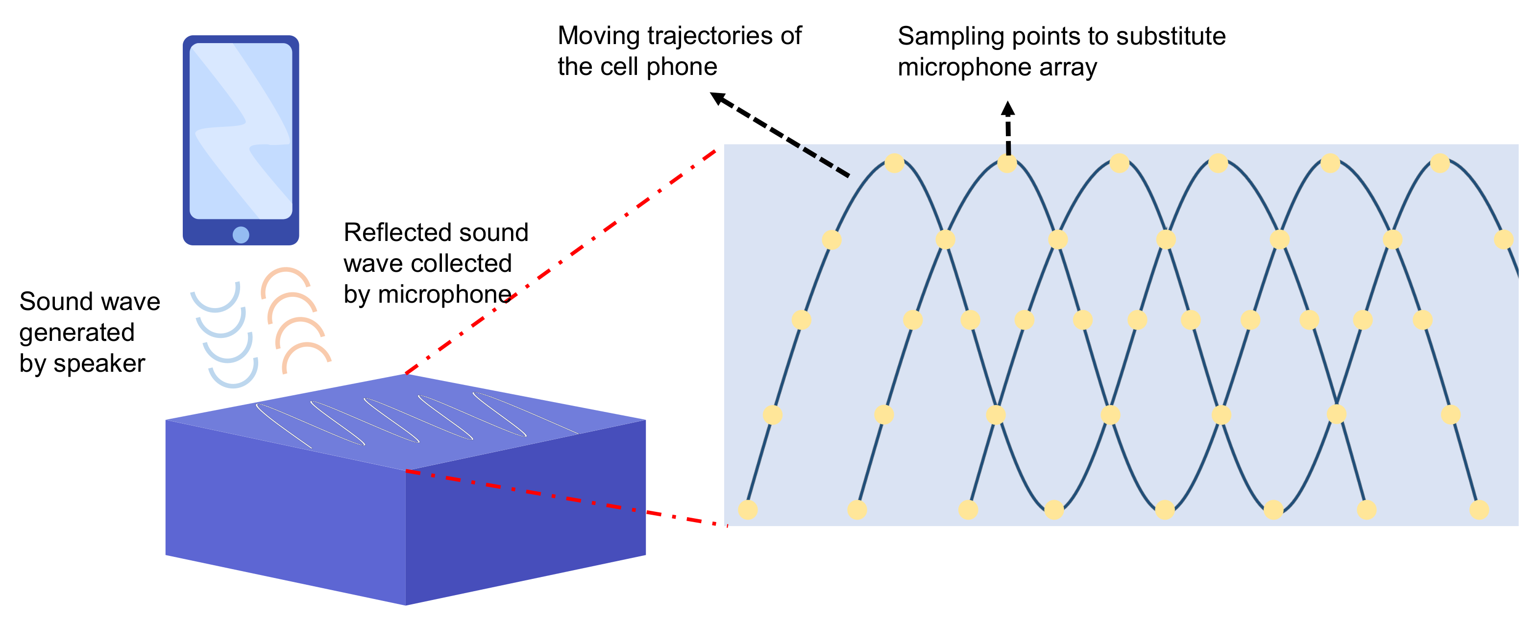
One fundamental issue needs to be overcome: the limited amount of microphones and speakers in a smartphone. Acoustic imaging usually uses the speaker and microphone array as the transmitter and receiver [22]. However, the number of microphones and speakers in a smartphone is usually less than five. For example, iPhone 12 has only two speakers (transmitter) and four microphones (receiver) [23]. To address this issue, we used the motion trajectory to replace the microphone array. A microphone plus an accelerometer become a symmetry imitation system that functions as the microphone array. As shown in Figure 1, the smartphone sweeps the surface of the object according to the prescribed route and the microphone collects reflected wave data at regular intervals. The light blue background indicates the surface of the object, the dark blue solid line indicates the prescribed route, and the yellow point indicates the sampling point. In this way, the sampling points on the trajectory constituted as a virtual microphone array (or so-called symmetry imitation system).
2.1. Overall Description of the Algorithm
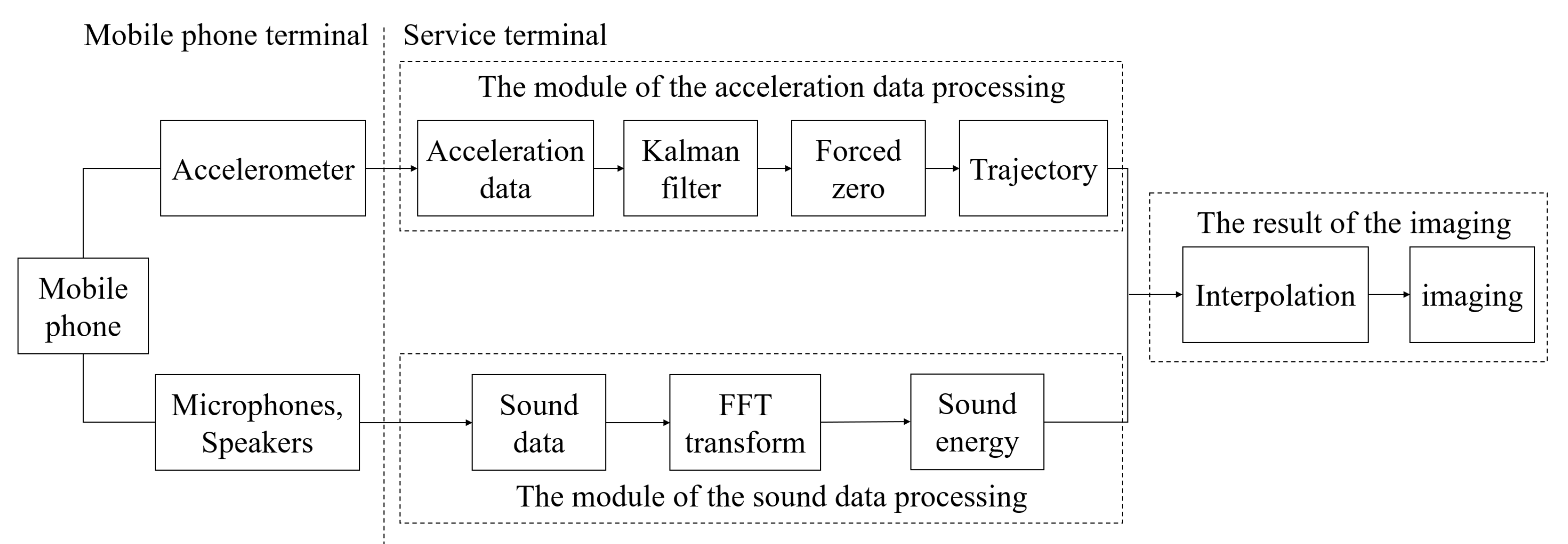
Based on the above analysis, our method provides a new solution to simplify the acoustic imaging algorithm to outline the contour of a target object. The processing flow of our method is summarized in Figure 2.
The algorithm shown in Figure 2 is composed of three modules: signals acquisition, data processing, and acoustic imaging. Cooperating with the built-in acceleration sensor, speakers, and microphones of a smartphone, we achieve acoustic imaging. The whole system is divided into two parts: the front end and the back end. The front end is constructed by HTML, which runs on the smartphone. The function of the front end is to call the built-in sensors on the smartphone to collect the acceleration data and reflected data. The back end is the server part. The algorithm of the data processing and acoustic image generation was implemented in the server (Centos 7.3, Intel Xeon E5-2680, 2.5 GHz, Santa Clara, CA, USA), for which the computing speed is 172 GFLOPS.
The working mechanism of our algorithm is described as follows. Starting from the end of the smartphone, the speakers of the smartphone acts as an active sound-generating device. It emits sound waves that contain a single or composite frequency band to the target object. After that, the reflected waves carrying the information of the object are collected by the microphones. Meanwhile, the accelerometer is used to collect the motion data in the process of scanning the object, which is further calculated to generate the motion track points. Finally, the reflected wave data are quantified as sound energy, which is mapped to the track points for visual expression to generate a two-dimensional acoustic image in the server end.
2.2. Data Acquisition Module
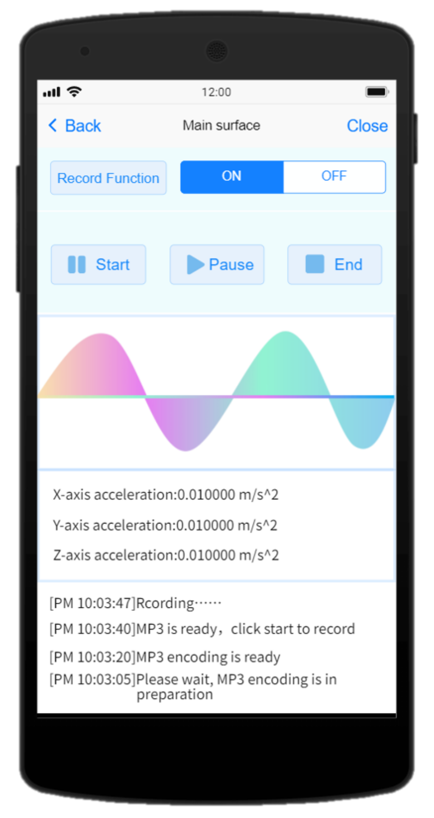
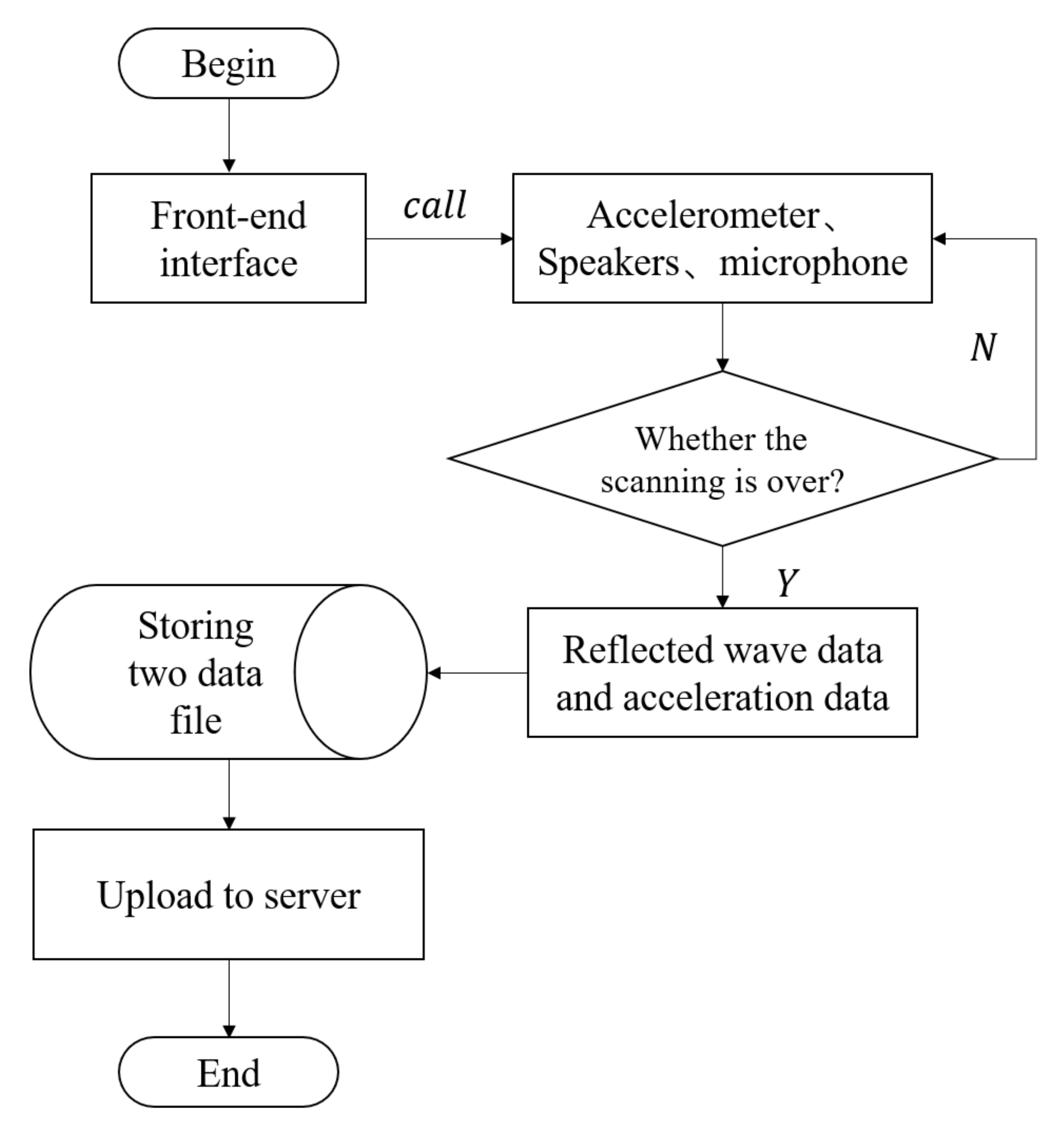
The data acquisition module provides a user-friendly interface (Figure 3) to control our imaging system, which can be accessed by https://chenmingbright.com/sum/assets/index.html (accessed on 28 April 2021). The smartphone model used for the experiment was Huawei P40 Pro (Android 10.0). After clicking the record button, the software turns on the speaker of the smartphone to emit sound waves of a 3 kHz frequency band and set the microphone to be ready for the incoming reflected waves. After that, the user clicks the start button to initialize the imaging process by recording the reflected wave and acceleration data. When the user starts to scan the target, the software automatically collects the waves reflected by the object under experiment as well as the trajectories provided by the acceleration data. When the smartphone moves, the main microphone at the bottom of the smartphone is aimed at the object, 2~3 cm away from the top of the object. The moving speed was ~0.065 m/s, which is relatively stable. Therefore, the amplitude change caused by human physiological jitter in the Z-axis direction can be negligible. The smartphone performs sinusoidal motion in the XY plane because the sinusoidal curve can cover the upper surface of the object to the greatest extent. It is able to ensure that enough effective data points are collected for acoustic imaging. The scanning process is also described in Figure 4. During the acquisition process, the reflected waves and acceleration data are stored in the local storage. After acquisition, the smartphone packages the cached data into a JSON format file and sends it to the server in a POST method.
2.3. Data Processing Module
There are inevitable errors in acceleration data and sound data collected by smartphone. Therefore, before processing them into trajectory and sound energy, the data need to be preprocessed to improve the accuracy of the final imaging. We used Fast Fourier transformation (FFT) [24], Parseval theorem [25,26], Kalman filter [27], and forced zero algorithm to calibrate the reflected wave and acceleration data.
2.3.1. Acceleration Data Processing
In the acceleration data processing module, we reduced the data error to an acceptable accuracy. Through the processed data, reconstruction of the trajectory of the smartphone movement is realized. The type of accelerometer used in the smartphone for testing is a MEMS-based sensor. Due to its own electrical and mechanical characteristics, there are three major types of errors from the MEMS-based accelerometer [28]. First, due to environmental temperature, magnetic field, etc., the acceleration data fluctuates around zero when the smartphone is stationary, which is called zero drift. In the other case, when the smartphone moves in a single direction, the acceleration data in the other direction have inertial fluctuations, which is called inertial drift. These two types of errors are defined as drift errors. Second, environmental electromagnetic changes or internal friction of sensor components produce unpredictable errors. These errors are defined as random errors. Third, during the movement of the smartphone, the tiny errors of the accelerometer continue to accumulate, which eventually creates a greater impact on the accuracy of the entire trajectory. These errors are defined as cumulative errors. Since the cumulative errors mainly come from the accumulation of drift errors and random errors, the cumulative errors can be reduced accordingly while reducing the other two types of errors.
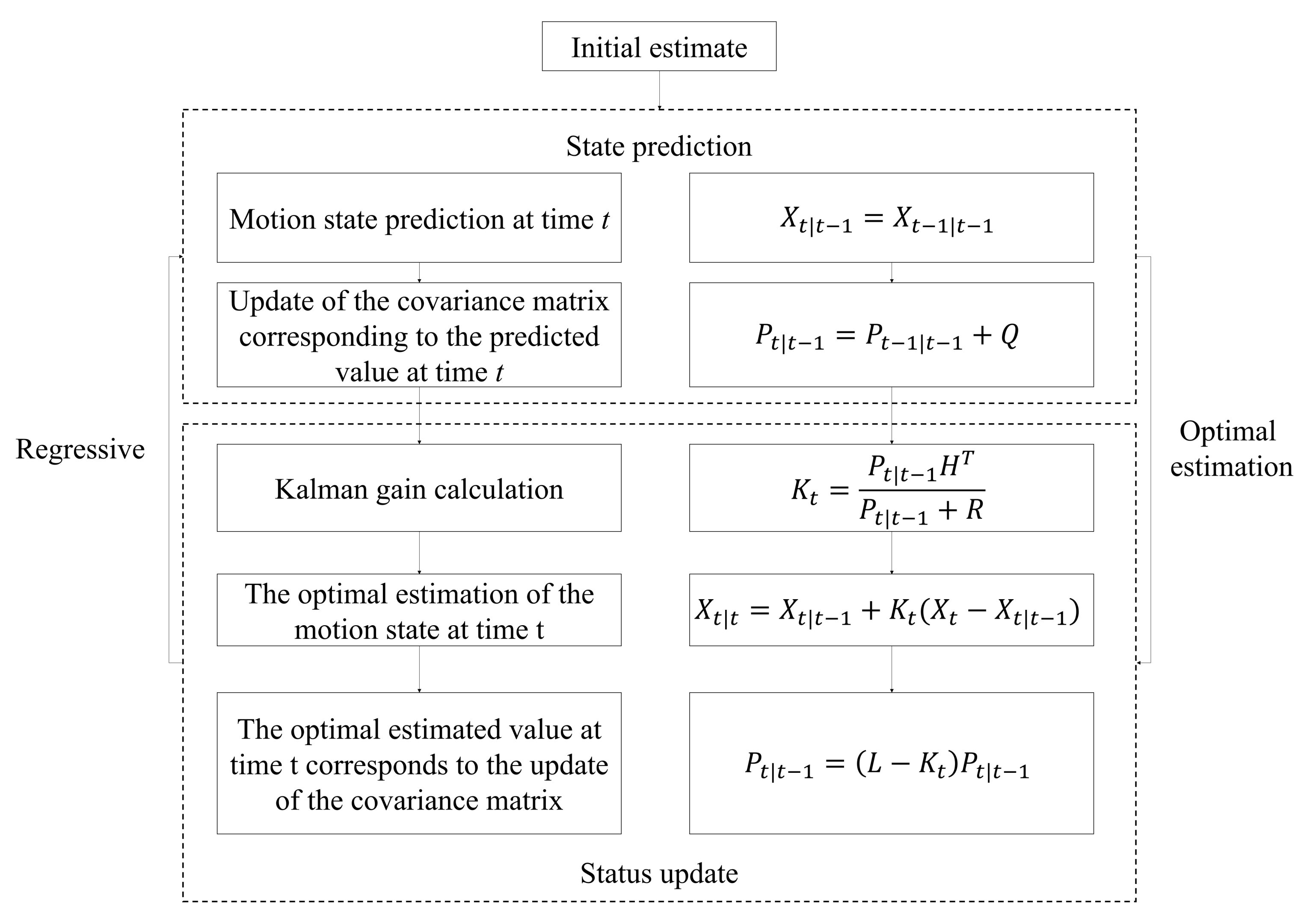
The random errors or so-called random noise is hard to predict [29]. Therefore, we need an effective algorithm to extract the signals from noise. In this work, the Kalman filter was chosen to eliminate the random noise. The Kalman filter is an efficient recursive filter [27]. Its basic idea is to bring the estimated value of the state at the previous moment and the observed value of the state at the current moment into the linear system state equations. In this way, the estimation of the state variables are updated and the state at the current moment is mostly estimated as well as calibrated. The Kalman filter uses continuous iteration, prediction, and correction methods to estimate the state of the dynamic system. Due to the fact that the observation data during the experiment includes random noise, the optimal estimation of the Kalman filter can be regarded as a filter process.
The Kalman filter includes two processes: state prediction and state update. Equations (1) and (2) express the state prediction:
where is the predicted result using the previous state of the system. means the optimal result that is processed by the Kalman filter at time . is the control function of the system, which is not defined during the experiment. Therefore, is set to 0. A is the state transition matrix. Since the sampling time of the sensor set in the experiment is 0.02 s. It is so short that the change between two adjacent states is negligible, so we set . The function of the Equation (1) is to use the motion state at time to predict the state at time t.
where is the error covariance matrix corresponding to , which is the same as to . Q is the covariance matrix of random noise errors in the motion process. It has components in the X and Y directions. In this way, Q can be expressed as . Set as an example; it is calculated as follows: accelerometer moves in the Y direction, the variance of the acceleration data measured when the X direction is stationary. According to the experiment, . is the transposed matrix of A. The function of Equation (2) is to use the error covariance matrix at time to predict the error covariance at time t.
Through the Equations (1) and (2), we can obtain the predicted state at current moment. Combining the prediction result with the actual observation value can obtain the optimal estimated value . Equations (3)–(5) are used to calculate how the next status is updated.
where is the Kalman gain. R is the random error covariance matrix of the sensor. Its value is the variance of the X-axis and Y-axis acceleration data measured in the static state, which is approximately equal to . Moreover, H is the parameter of the measurement system. Since the MEMS sensor integrated in the smartphone is calibrated by the sensor manufacturer, the observed value measured by the sensor reflects the current motion state of the sensor. Therefore, we set , where indicates the transposed matrix of H.
where means the optimal result processed by the Kalman filter at time t. The function of Equation (4) is to use the estimated value at time t to calibrate the measured value at time t.
where L presents the identity matrix. The function of Equation (5) is to use , which is the error covariance matrix corresponding to , to update the error covariance matrix . When the system enters time , is updated to in Equation (2), so that the algorithm autoregressively calculates until the system process ends.
The optimal estimation process of the system motion state mentioned above can be regarded as a process of filtering. It could remove the noise and interference in the system, which is capable of reducing random errors. The flowchart of the Kalman filter is further described in Figure 5.
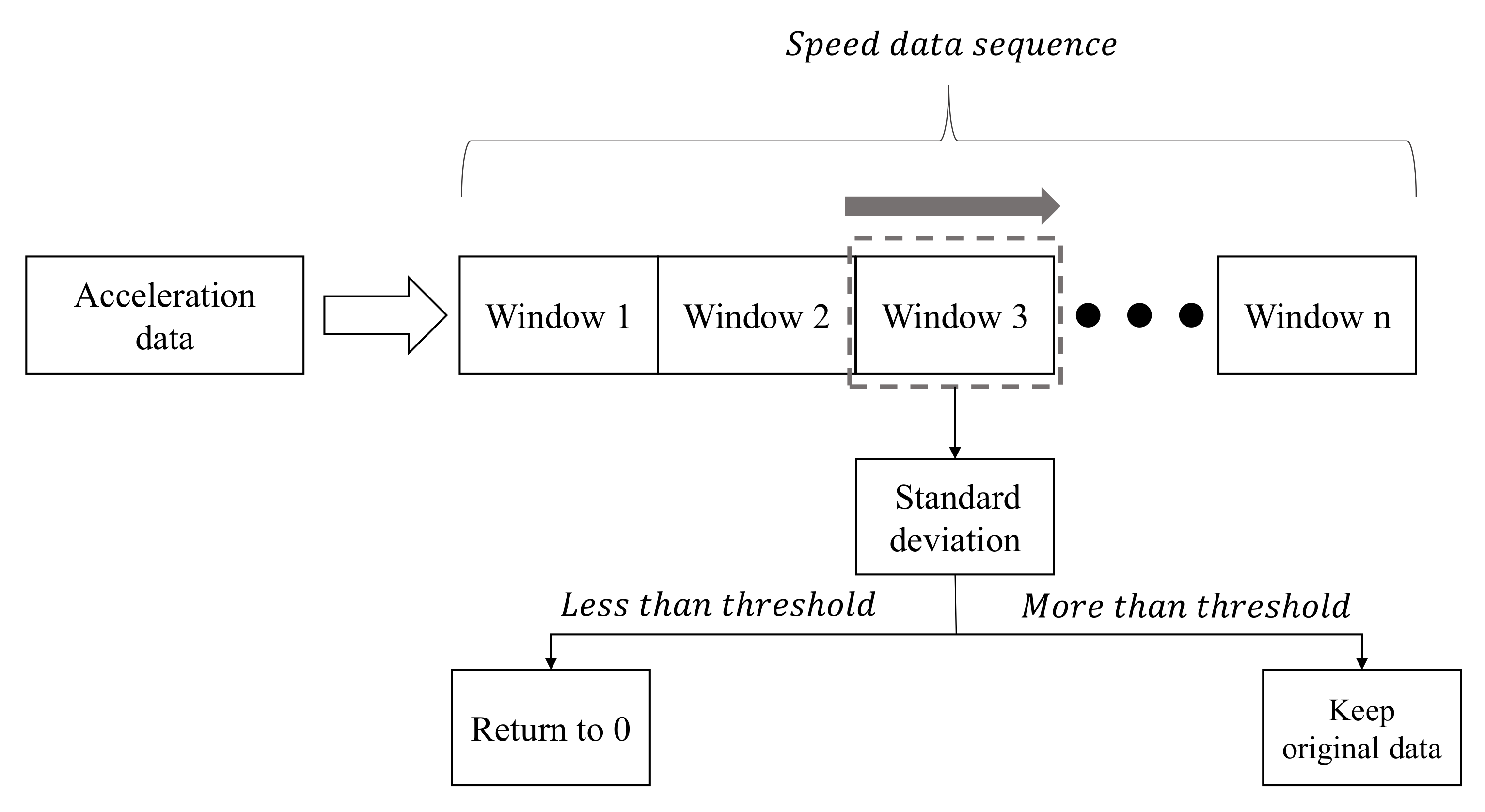
Apart from the Kalman filter, we also use a forced zero algorithm to suppress the drift errors of the system, including zero drift and inertial fluctuation. In general, the fluctuation of the acceleration data causes a large error in the speed calculation, thereby affecting the calculation of the trajectory. We designed a forced zero algorithm to reduce the error of speed caused by the above two drift errors.
As shown in Figure 6, first, the acceleration data are used to calculate the velocity at each sampling time. The acceleration data has components in the X and Y directions. The data in each direction are processed separately. Set the X direction as an example:
where and are the velocity values at the current time and the previous time in the X direction, respectively. is the acceleration in the X direction, and T is the sampling period. Using 20 sampling points as a window, we can calculate the standard deviation of the speed in each window:
where means the ith point at the current window and the r is the average of 20 points speed data. Moreover, the presents the velocity of the ith point.
With the standard deviation as the threshold, the program traverses all of the windows. If the standard deviation of this window is less than , all of the data in this window are returned to zero. The acceleration data in the X and Y directions are processed as described above, and we obtained the speed data with smaller errors in the two directions.
After using the Kalman filter and the forced zero algorithm, we obtain the speed data of the smartphone along the X and Y directions at each sampling point. Additionally, the error of the speed data is suppressed to a certain extent, which is able to rebuild the trajectory. Since the time interval between two adjacent sampling points is short enough, the motion between two adjacent points can be approximated as a uniform linear motion. Additionally, the speed is the average value of that at the two adjacent sampling points. Using the speed data in the two directions, we can calculate the displacement in each sampling period and its accumulation over time.
The displacement within a certain sampling period in a certain direction is expressed by Equation (8):
where is the displacement within a sampling period. and indicate the velocity values at time t and , respcetively. T is the sampling period. The cumulative value of the displacement from time 0 to the sampling point (time t at current) in a certain direction is expressed by Equation (9):
where the meaning of is the same as . represents the displacement from time to t. Combining Equations (8) and (9), we are able to obtain the total displacement of each sampling point of the smartphone in a single direction. Finally, the two sets of data are drawn on a two-dimensional plane and combined orthogonally to obtain the motion trajectory of the smartphone.
2.3.2. Reflected Wave Data Processing
After completing the trajectory reconstruction, we need to process the reflected wave signal. The errors of reflected wave data mainly come from two aspects: (1) The reflected wave is affected by environmental noise, such as reflected echo. Theoretically, the sound received by the microphones appear as an overlapping wave. (2) The sound energy is attenuated by the square of the distance during transmission and reception.
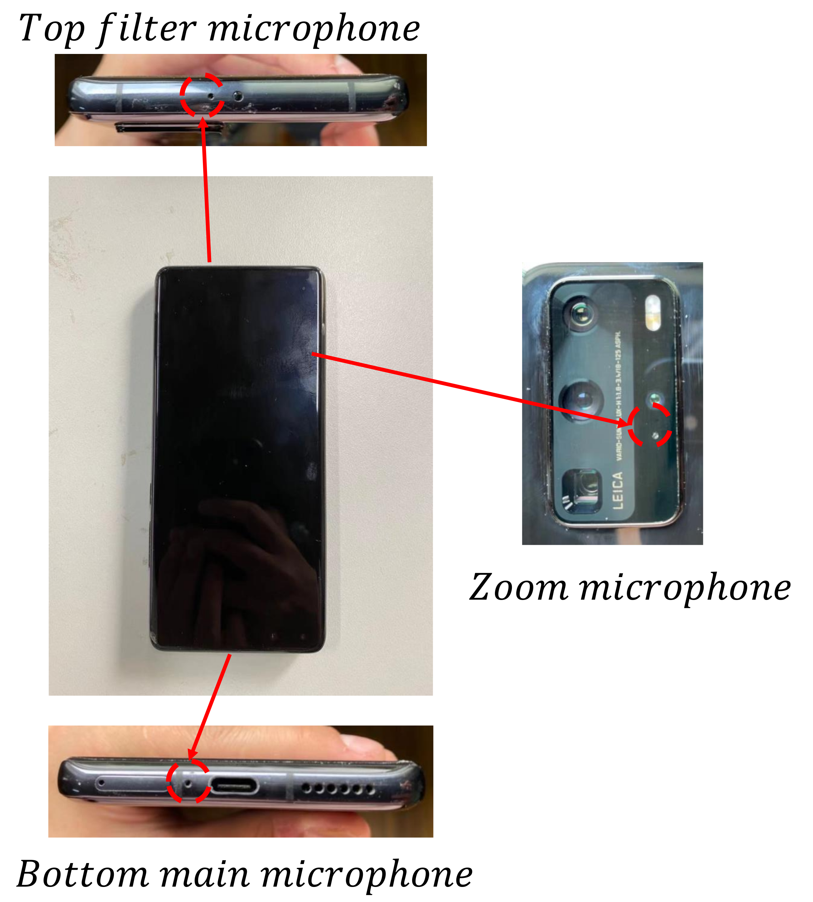
For the first question, we combined the method of smartphone self-calibration and selection of the best sound wave. As show in the Figure 7, it is a distribution map of the microphones in the smartphone that we used for the experiment.
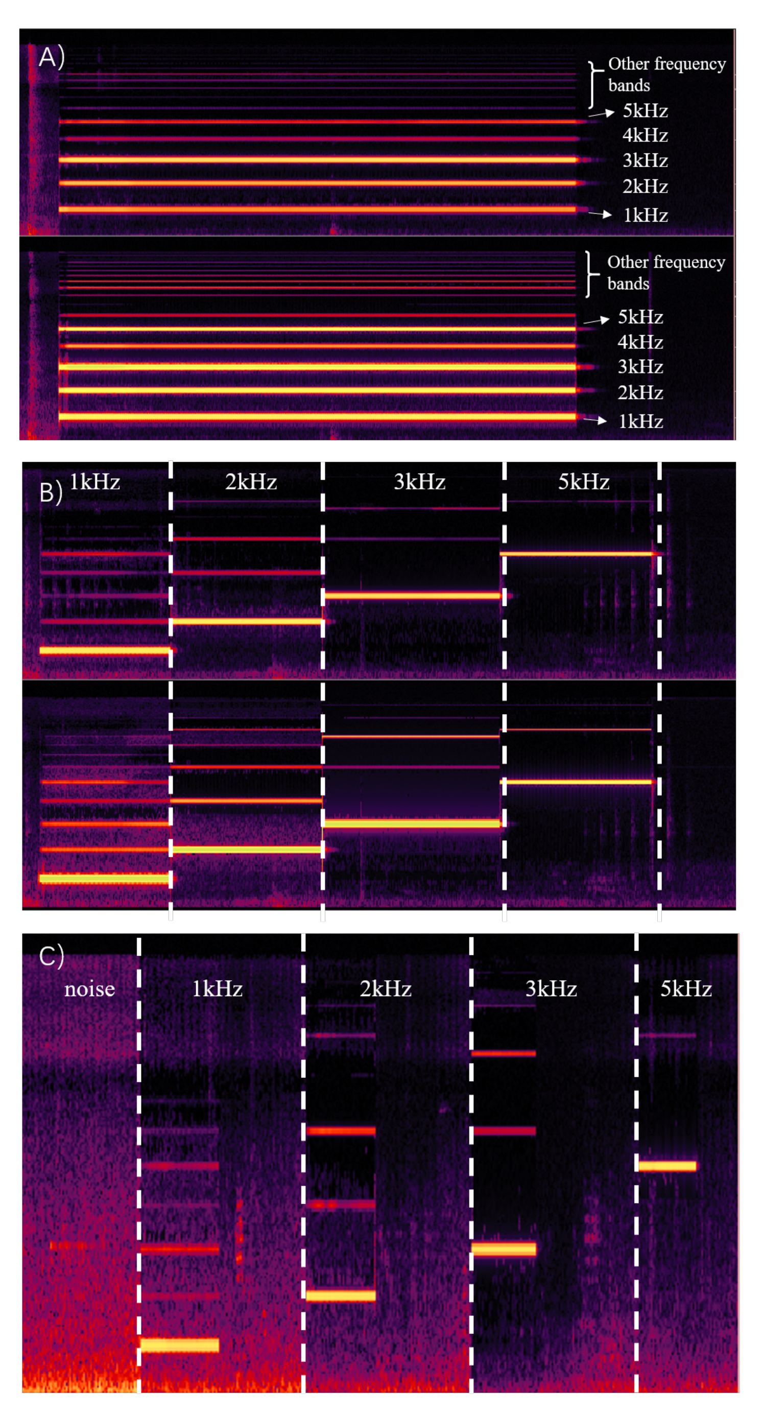
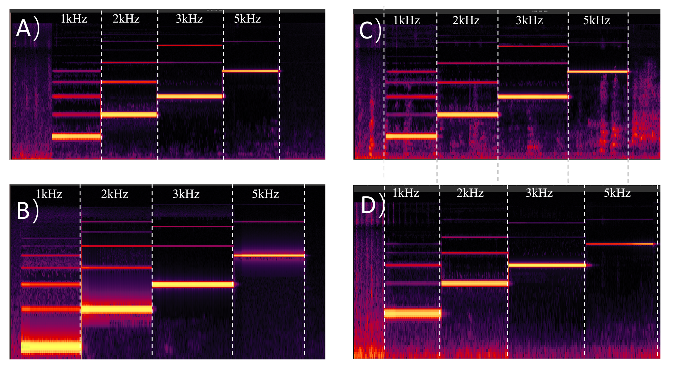
There are three microphones. The main one is at the bottom, recording the reflected wave at the sound source. The second one is the top filter microphone, recording the noise and the attenuated wave from the sound source. The third zoom microphone is located in the camera module. When the phone recording function and call function work, the top and bottom microphone work by default. In the system that we designed, the bottom microphone is used to record the 3 kHz sound waves reflected from the sound source. The top filter microphone records reflected waves outside the sound source and background noise. The smartphone has built-in sound signal processing algorithms [30]. The algorithm detects the sound source and processes the noise based on the power of the sound signals recorded by the two microphones. After the self-filtering process of the smartphone, the signal recorded by the smartphone retains the sound source to the greatest extent and filters other noises. These algorithms are designed by manufacturers to ensure the quality of a call and are relatively mature. In addition, we tested the sound waves in the best audible frequency band to maximize the signal collected at the sound source. We built a sound wave with a composite frequency band, the range of which is from 1 kHz to 20 kHz. As shown in Figure 8, the sound wave in the 3 kHz frequency band is the most obvious in the reflected waves. It means that selecting a 3 kHz frequency band can minimize the impact of environmental noise.
As for the solution to error type two, the method we used is close-range scanning and dense sampling. The amplitude of the sound signal is attenuated with the square of the distance [31]. We set the smartphone to be 2~3 cm away from the object in the experiment. As a healthy human hand’s physiological jitter in the Z-axis direction is less than 0.2 cm, we assume that the smartphone is stationary in the Z-axis. Moreover, dense sampling points can ensure that a sufficient amount of data are collected. As the smartphone is a highly integrated device, the internal sensors cannot be controlled by the user at will, unlike a microphone array. What we are able to do is to enhance the target sound and to optimize the physical environment. The combination of the two methods mentioned above compensates for the sound energy loss.
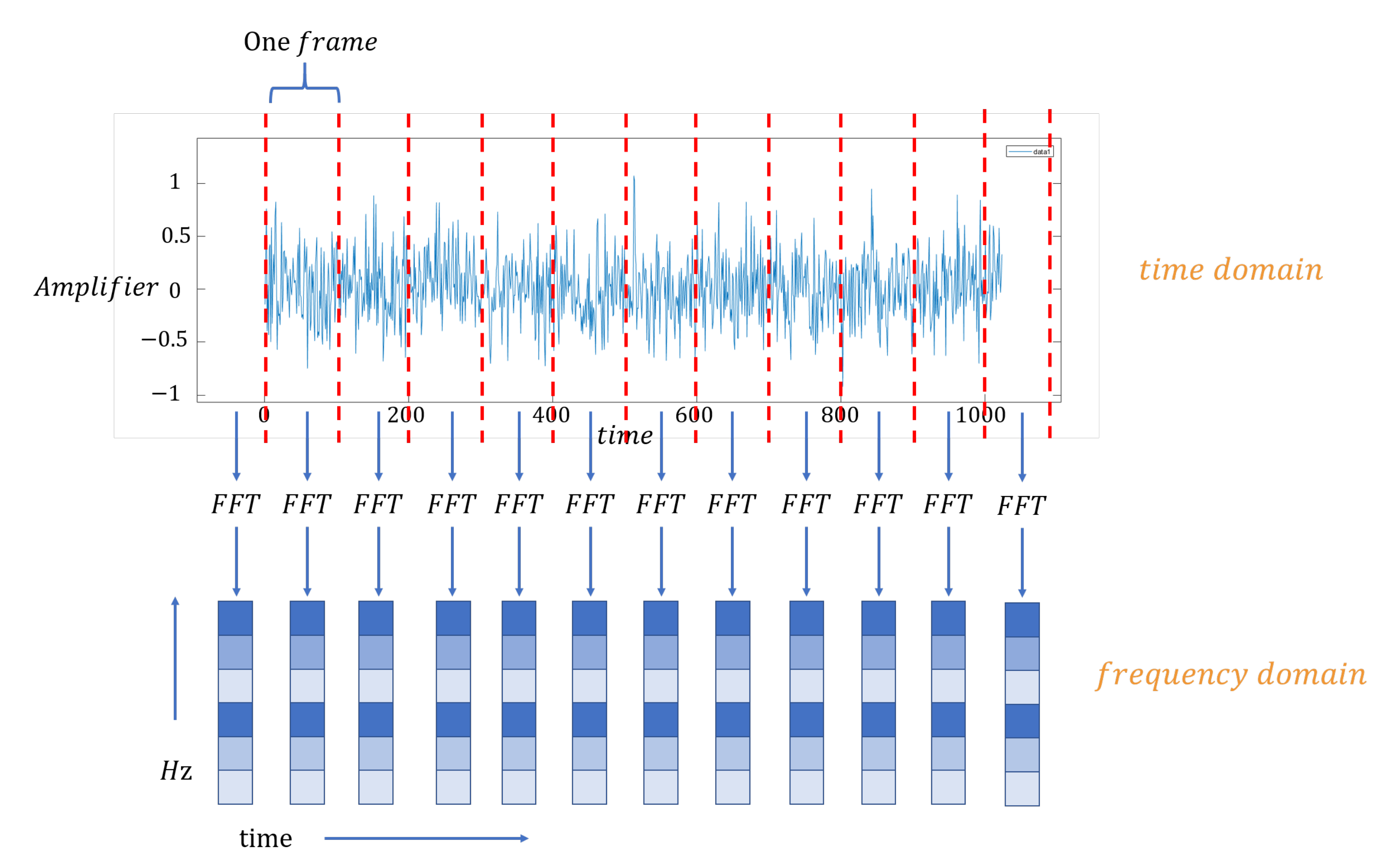
To facilitate the subsequent sound energy calculation, the sound data collected and stored by the microphones are first converted from the time domain to the frequency domain. As the collected sound signal is a discrete signal, each frame of sound needs to be processed by Fast Fourier transformation (FFT) and converted into a frequency domain representation:
where is the signal value of the nth sampling point in one frame in the time domain. is a rotation factor, which is defined as shown in Equation (11). is an expression of complex numbers in FFT transformation. is the value of the kth signal in one frame after FFT. is a complex number. Through the argument and modulus, algorithm can calculate the frequency and amplitude.
where N is the total number of the sampling points in one frame. Taking into account the computational time complexity, the FFT algorithm used in the code design is able to obtain the amplitude and phase of each frequency component decomposed from each frame of sound signal rapidly. The process of FFT is shown in Figure 9. The program divides the sound signal into frames. Each frame is performed by FFT to transform the signal from the time domain to the frequency domain. This process is implemented by the FFT function in the Librosa library or the NumPy library of the Python. The result of the function execution can be a list containing each frequency component and the corresponding intensity.
After completing the transformation, we selected the frequency component of 3 kHz for further calculation. As 3 kHz is the test frequency band, this selection process can be regarded as filtering. The FFT size that we used for the experiment was 1024, and the sampling frequency was 20 kHz. Then, we used the Parseval theorem [26] to convert the sound energy calculation of one frame into the frequency domain because frequency filtering is easier in the frequency domain. The total energy of the signal was calculated according to the integral of the energy per unit time over the entire time or according to the energy per unit frequency integrated over the entire frequency range.
where is the same as in Equation (10). Using Equation (12), the energy of the sequence in the time domain is equal to its energy in the transform domain, which is the sum of the power of each harmonic.
As for the Fourier series of a complex exponential form, its energy value can be directly calculated by the square of the modulus of the coefficient. Therefore, the short-time average energy is expressed as Equation (13):
where represents the short-time average energy of the ith frame. represents the signal amplitude of the kth frequency component of the ith frame, and N is the total number of all frequency components in the ith frame.
2.3.3. Acoustic Imaging
Now, we obtained the “microphone array data” based on the moving trajectory and sound energy data. At this point, how should we combine these two data to generate an acoustic image? First, we matched the sound energy with the track points data in that the number of the sound energy was different from the track points. The audio sampling frequency we set was 48 kHz, and the number of samples in one frame was 384. We used the MP3 format to store the wave file. It is a lossy compression, but the frequency band it compressed is the high part (greater than 20 kHz) [32]. Therefore, the time contained in one frame is ms and the total number of frames of sound energy collected for 1 s is 1 s ms frames. However, the sampling time of the trajectory points was 0.02 s. Hence, the number of the trajectory points is 50. The total number of sound energy data is larger than the number of trajectory points in the case of the same length of time. To solve the problem of quantity mismatch, we took the number of track points as the number of windows and then summed the sound energy in a window as the sound energy corresponding to the trajectory point.
Regarding the rationality of the processing method, we first summed the sound signals into a period of time as the sound energy at corresponding point. As the sampling speed of the sound signal is 48,000 Hz, the sampling speed is fast. Therefore, the sound signal exhibits continuous characteristics in the time domain. The sampling of our trajectory signal is 0.02 s, which makes the trajectory almost a continuous curve even though it is depicted by a scatter diagram. For two consecutive signals, as long as the start and end times are the same, we can match them in the time domain. The other treatment is the audio delay between two sampling points. As we know, the propagation speed of sound waves under a standard atmospheric pressure is 340 m/s while the speed of the smartphone in the experiment is 0.065 m/s. The error due to the time delay is . Under the condition that high precision is not required, this error is negligible. After completing the matching process, the sound energy was mapped to the track point and we obtained a curve with energy distribution.
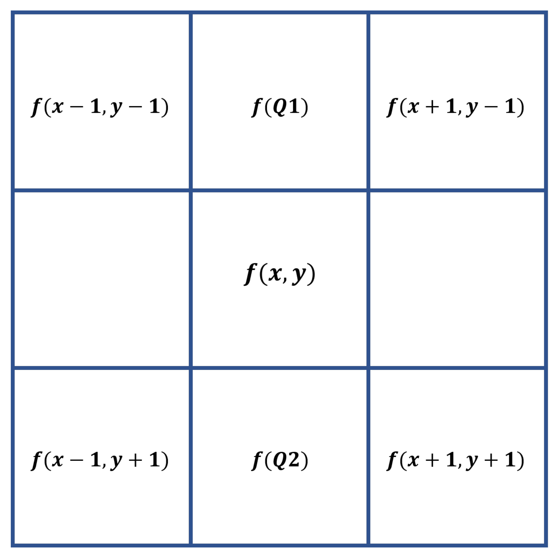
However, what we wanted to show in the end is a two-dimensional plane with energy distribution, not a trajectory. Therefore, we used bilinear interpolation [33] to complete the trajectory. Bilinear interpolation is calculated by using the correlation of four pixels around the original image pixel to be processed.
As shown Figure 10, we expected to obtained the sound energy of . Hence, we selected the four pixels closest to the coordinates . The bilinear interpolation algorithm stipulates that the nearest neighbor points are the upper left, lower left, upper right, and lower right of the pixel. First, we input the sound energy of the four closet points into Equations (14) and (15) to obtain the value of :
where is the pixel value, reflecting the sound energy of the coordinate . is equal to , and is equal to . Then, putting and into Equation (16), we obtained the value of :
where is equal to y + 1 and is equal to .
In order to verify the rationality of the bilinear interpolation algorithm, we carried out theoretical calculations. The concept map is shown in Figure 11.
The squares in the background represent pixels, and the orange curve is the trajectory curve of the smartphone scanning the human hand. We set points A and B as an example, and points A and B have no trajectory passing. Therefore, we estimated the pixel values of the two points through bilinear interpolation. The coordinates and sound intensity assumptions of points A and B and their adjacent points are shown in Table 1:
3. Results and Discussion
The smartphone models we used for the experiment were Huawei P40 Pro (Android 10.0) and iPhone 12 (IOS 14). The experimenter was in good health and had no related diseases that could cause severe hand shaking.
3.1. Determination of the Frequency Band of Sound Waves
The frequency band of sound waves that smartphones can emit is limited to 20 kHz, and the reflected waves interfere with each other. To solve this issue, we built a mixed wave with a frequency band from 1 kHz to 20 kHz to determine which frequency of sound waves should be used for our algorithm. As shown in Figure 8, in the composite frequency band test (Figure 8A), the sound wave in the low frequency band was more obvious in the reflected wave. Therefore, we conducted a single band test on the four frequency bands (1 kHz, 2 kHz, 3 kHz, and 5 kHz) with a strong reflection. This test was performed on a smooth table. In the single frequency band test (Figure 8B), 3 kHz suffers less interference from other frequencies. These two tests showed that the 3 kHz frequency band retains the reflected wave carrying the object information to the maximum. In addition, in order to verify the noise reduction performance of the mobile phone, as described in Section 2.3.2, we conducted a single-band test of short impulse tones in a noisy environment. The result is shown in Figure 8C; before the main sound source appears, the microphone records the noise in the environment. After the main sound source (1k, 2k, 3k, and 5k) appeared, the background noise was obviously suppressed.
In order to verify the general applicability of the experimental conclusion, we supplemented the single-frequency test with three aspects: reflect surface, the smartphone system, and the environment. As shown in Figure 12, under most of the test conditions, the 3 kHz reflected wave data was well preserved and the 3 kHz frequency band was relatively clean. Therefore, the 3 kHz frequency band used in our experiment is a good example.
3.2. Reconstruction of Trajectories from the Motion of the Smartphone
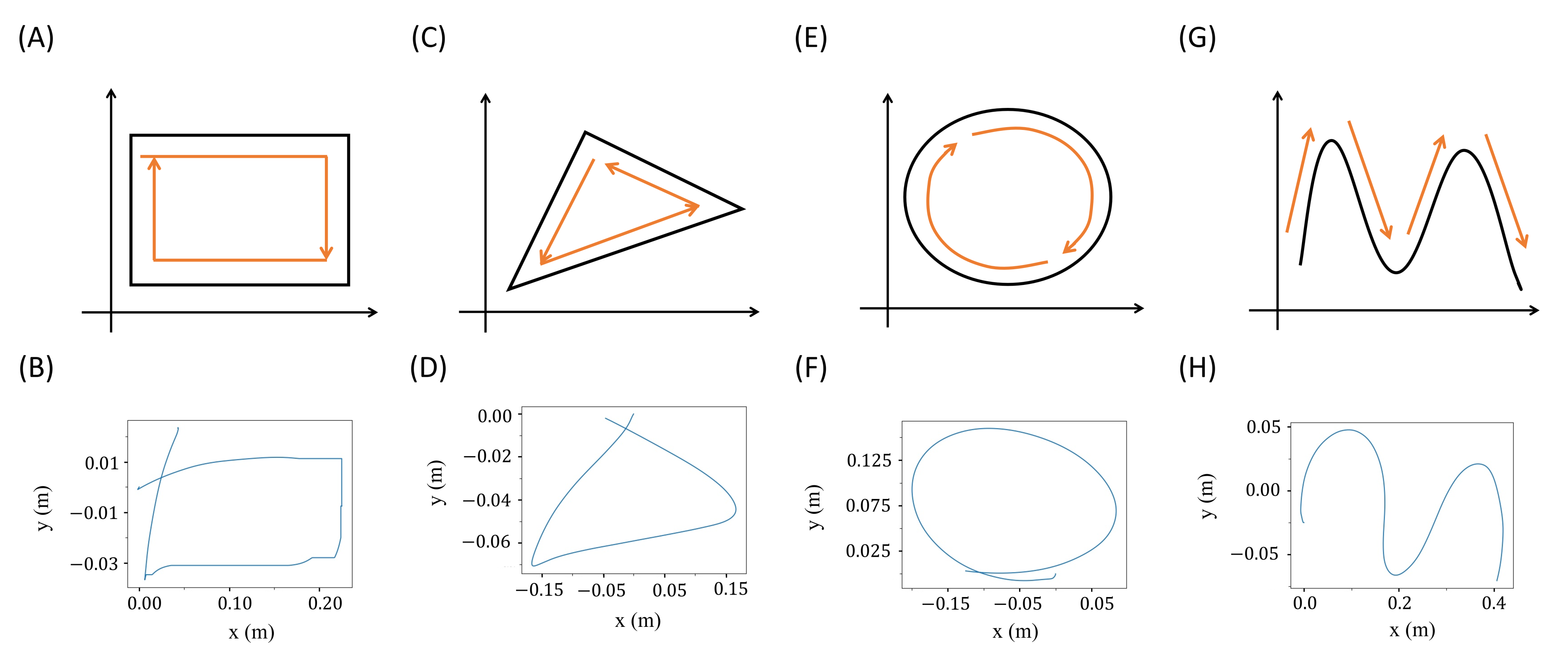
After two filtering processes, the acceleration data was calculated as the trajectory points using Newton’s second law of motion. In order to test the effect of trajectory reconstruction, we used basic graphics including a rectangle (Figure 13A) with its algorithm outlined trajectory (Figure 13B), a triangle (Figure 13C) with its algorithm outlined trajectory (Figure 13D), a circle (Figure 13E) with its algorithm outlined trajectory (Figure 13F), and a sinusoid (Figure 13G) with its algorithm outlined trajectory (Figure 13H) to test our algorithms. From the four generated trajectories, this algorithm reconstructed the trajectory curve from smartphone movement perfectly. After the analysis, the experimental error was within 10%, which meets the requirements of subsequent imaging.
In the speed trajectory reconstruction, the sensor called by the smartphone was only the accelerometer. It was calibrated by the smartphone manufacturer before leaving the factory. Unless in a strong geomagnetic environment or subjected to a serve impact, the accelerometer works normally. Therefore, realization of the trajectory reconstruction part is scalable under different physical conditions and different platforms.
3.3. Acoustic Imaging
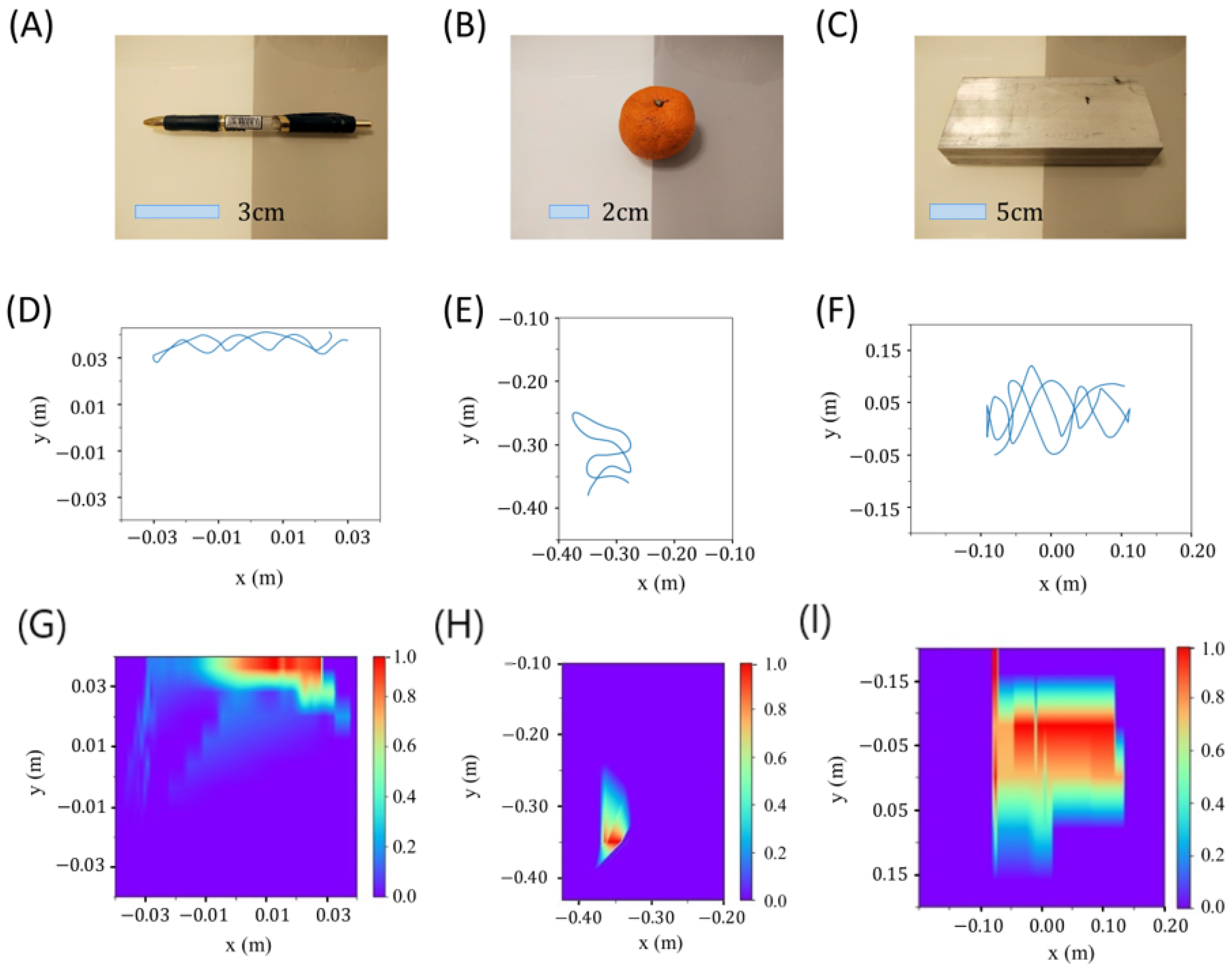
After the preliminary data processing, the acceleration data and the reflected wave data were processed into trajectories and sound energy, respectively. Then, these two data were matched and interpolated through the acoustic imaging module. As shown in Figure 14, we scanned a pen (Figure 14A), an orange (Figure 14B), and a piece of aluminum (Figure 14C). Figure 14D–F show the corresponding trajectories. The scanning area covers the area where the object is located but is not a large-scale scan. This is because the accelemeter of the smartphone is a capacitive sensor, and there is a spring inside that connects a mass and a plate. The compression or extension of the spring during the movement causes the capacitance to change. Thus, the acceleration can be measured. If the scanned area is too large, it is difficult for the experimenter to control the movement state of the hand, which easily leads to sudden changes. In addition, our smartphone adopts an approximate sine curve motion and the trajectory covers the surface of the object as many times as possible. The trajectory of the sine curve is not prone to sudden changes in one direciton, and multiple coverages can ensure that enough reflected wave information is collected. If the trajectory passes through a point repeatedly, the program updates the value of that point. The final imaging result is shown as Figure 14G–I. The imaging algorithm first generates a low-resolution (few pixels) image matrix, which allows for most of the pixel blocks to have trajectories passing by. Then, the matrix was interpolated many times to generate a high-resolution picture. In order to facilitate observation, we expanded the background of the result graph (the part where the sound energy is 0 in purple). For the part with sound wave reflection, the basic contour of the scanned object was able to be observed in the part with a heating value . The parts with heating values between 0.2 and 0.6 were the desktop scanned during the movement. The desktop is far from the smartphone, and the radiation received waves are relatively weaker than the surface of the object. Although the image quality cannot be comparable with commercial equipment, it outlined the general shape of the three target objects. From the effect diagram of acoustic imaging, the algorithm designed in this paper can reconstruct the outline of simple objects.
Moreover, we compared the results achieved by SAR based on the audible frequency band.
(1) From the results, our algorithm also achieved acoustic image under the sound wave condition in the audible frequency band. The imaging results can roughly identify the shape and the size of the object. Our accuracy is between 60% and 90%, while the accuracy of the SAR-based method is between 70% and 90%. This proves the feasible of our algorithm to use the audible frequency band for acoustic imaging.
(2) In terms of implementation method, the system based on SAR uses the movement of the device to simulate an antenna to replace the microphone array. The algorithm performs coherent processing on echoes received at different locations to obtain high-resolution acoustic images. SAR needs to locate the sound source of the reflected wave, which involves phase correction, interference cancellation, and filtering. This approach is able to work out high-quality images, but its implementation logic is more complicated. Our algorithm uses the sampling points on the trajectory to directly simulate the real microphone array, which becomes a symmetry imitation system. Since the distance between the object and the smartphone is 2~3 cm, we assumed that the sampling point and the sound source are correspondent. Therefore, we do not need to locate the sound source point. Moreover, the best sound wave test and the smartphone’s self-filtering algorithm ensures that the reflected waves carry the correct information. The algorithm implementation logic is simple. Furthermore, we compared the performance of the smartphone processor (Kirin 990, greater than 7 TOPS) and sever processor (Intel Xeon E5-2680, 172 GFLOPS), which verifies that the feasibility of transplantation of data processing and acoustic imaging algorithms to a smartphone is high. However, our algorithm exhibits strong randomness in experiments. We speculate that it is due to the limitation of the physical properties of the sensors.
4. Conclusions
This paper presents an acoustic imaging algorithm to outline the contour of a target using the built-in sensors of a smartphone. The core idea is to use the smartphone motion trajectory instead of a microphone array by leveraging the idea of a symmetry imitation system. Using the built-in sensors, a smartphone is able to send and receive sound wave signals as well as reflected waves. In this way, the smartphone itself is a transceiver. Meanwhile, the accelerometer in the smartphone collects the motion data. After uploading the data to the server, the data is preprocessed by the Kalman filter and Parseval theorem. Finally, the processed trajectory and sound energy data are interpolated to obtain an acoustic image with energy distribution.
In summary, our work explores the possibility of using a smartphone to achieve acoustic imaging as well as the corresponding algorithms. The experimental demonstration is feasible but the current accuracy is low, which is due to the limitations of the smartphone’s hardware conditions. In further research, we will design adaptive algorithms such as attitude angle fusion and reflected wave distance calculation methods for dynamic calibration of data acquisition during movement. It will help compensate for the defects of the hardware and will improve the imaging accuracy. Moreover, based on our discussion of the computing speed between sever and smartphone, we also plan to transplant the entire algorithm implementation program to a smartphone to realize a completely phone-based acoustic imaging approach.
Author Contributions
Conceptualization, C.L. and J.W.; methodology, C.L.; software, C.L.; writing—review and editing, C.L., X.D., N.Z., and J.W. All authors have read and agreed to the published version of the manuscript.
Funding
This research was funded in part by the Zhejiang Provincial Natural Science Foundation of China under grant No.LQ20F040003 and by Fundamental Research Funds for the Provincial Universities of Zhejiang No.GK209907299001-028.
Informed Consent Statement
Not applicable.
Data Availability Statement
Not applicable.
Conflicts of Interest
The authors declare no conflict of interest.
References
- Koch, W.E. Sound visualization and holography. Phys. Teach. 1975, 13, 14–22. [Google Scholar] [CrossRef]
- Yu, X.; Zhang, Y. Sense and avoid technologies with applications to unmanned aircraft systems: Review and prospects. Prog. Aerosp. Sci. 2015, 74, 152–166. [Google Scholar] [CrossRef]
- Sutton, J.L. Underwater acoustic imaging. Proc. IEEE 1979, 67, 554–566. [Google Scholar] [CrossRef]
- Yu, S.; Zhang, X.; Zhang, B.; Kong, B. Research on inversion and application of failure depth of coal seam roof and floor based on triangular network acoustic CT tomography. Environ. Earth Sci. 2020, 79, 1–14. [Google Scholar] [CrossRef]
- Sarvazyan, A.P.; Urban, M.W.; Greenleaf, J.F. Acoustic waves in medical imaging and diagnostics. Ultrasound Med. Biol. 2013, 39, 1133–1146. [Google Scholar] [CrossRef] [PubMed] [Green Version]
- Wall, A.T.; Gee, K.L.; Neilsen, T.B.; McKinley, R.L.; James, M.M. Military jet noise source imaging using multisource statistically optimized near-field acoustical holography. J. Acoust. Soc. Am. 2016, 139, 1938–1950. [Google Scholar] [CrossRef]
- Fernandez Comesana, D. Scan-Based Sound Visualisation Methods Using Sound Pressure and Particle Velocity. Ph.D. Thesis, University of Southampton, Southampton, UK, 2014. [Google Scholar]
- Huang, X.; Bai, L.; Vinogradov, I.; Peers, E. Adaptive beamforming for array signal processing in aeroacoustic measurements. J. Acoust. Soc. Am. 2012, 131, 2152–2161. [Google Scholar] [CrossRef] [Green Version]
- DAWEI. China Hot Sell DW-T6 Portable 4d Baby Color Doppler Ultrasound Scan Machine for Women’s Health Manufacturers and Suppliers|Dawei. Available online: https://www.ultrasounddawei.com/t6-4d-baby-color-doppler-ultrasound-scan-machine-product/ (accessed on 4 May 2021).
- Thompson, S.E.; Parthasarathy, S. Moore’s law: The future of Si microelectronics. Mater. Today 2006, 9, 20–25. [Google Scholar] [CrossRef]
- Bogue, R. Recent developments in MEMS sensors: A review of applications, markets and technologies. Sens. Rev. 2013, 33, 300–304. [Google Scholar] [CrossRef]
- Tanaka, M. An industrial and applied review of new MEMS devices features. Microelectron. Eng. 2007, 84, 1341–1344. [Google Scholar] [CrossRef]
- Semianalysis. A14 Packs 134 Million Transistors. Available online: https://semianalysis.com/apples-a14-packs-134-million-transistors-mm2-but-falls-far-short-of-tsmcs-density-claims/ (accessed on 4 May 2021).
- PCPOP. A12, Kirin 980, Snapdragon 855 Performance Competition, How Much Difference Can be between the Top Flagships. Available online: http://www.pcpop.com/article/5178582.shtml (accessed on 25 May 2021).
- Hanilçi, C.; Ertas, F. Optimizing acoustic features for source cell-phone recognition using speech signals. In Proceedings of the First ACM Workshop on Information Hiding and Multimedia Security, Montpellier, France, 17–19 June 2013; pp. 141–148. [Google Scholar]
- Zhang, L.; Tian, Z.; Bachman, H.; Zhang, P.; Huang, T.J. A Cell-Phone-Based Acoustofluidic Platform for Quantitative Point-of-Care Testing. ACS Nano 2020, 14, 3159–3169. [Google Scholar] [CrossRef]
- Wang, Z.; Tan, S.; Zhang, L.; Yang, J. ObstacleWatch: Acoustic-based obstacle collision detection for pedestrian using smartphone. ACM 2018, 2, 1–22. [Google Scholar] [CrossRef]
- Pradhan, S.; Baig, G.; Mao, W.; Qiu, L.; Chen, G.; Yang, B. Smartphone-based acoustic indoor space mapping. ACM 2018, 2, 1–26. [Google Scholar] [CrossRef]
- Mao, W.; Wang, M.; Qiu, L. Aim: Acoustic imaging on a mobile. In Proceedings of the 16th Annual International Conference on Mobile Systems, Applications, and Services, Munich, Germany, 10–15 June 2018; pp. 468–481. [Google Scholar]
- Izquierdo, A.; Villacorta, J.J.; del Val Puente, L.; Suárez, L. Design and evaluation of a scalable and reconfigurable multi-platform system for acoustic imaging. Sensors 2016, 16, 1671. [Google Scholar] [CrossRef] [PubMed] [Green Version]
- Legg, M.; Bradley, S. Automatic 3D scanning surface generation for microphone array acoustic imaging. Appl. Acoust. 2014, 76, 230–237. [Google Scholar] [CrossRef]
- Bjelić, M.; Stanojević, M.; Šumarac Pavlović, D.; Mijić, M. Microphone array geometry optimization for traffic noise analysis. J. Acoust. Soc. Am. 2017, 141, 3101–3104. [Google Scholar] [CrossRef]
- APPLE. AiPhone 12 and iPhone 12 Mini—Apple (SG). Available online: https://www.apple.com/sg/iphone-12/ (accessed on 4 May 2021).
- Cochran, W.T.; Cooley, J.W.; Favin, D.L.; Helms, H.D.; Kaenel, R.A.; Lang, W.W.; Maling, G.C.; Nelson, D.E.; Rader, C.M.; Welch, P.D. What is the fast Fourier transform? Proc. IEEE 1967, 55, 1664–1674. [Google Scholar] [CrossRef]
- Hu, L.-Y.; Fan, H.-Y. Inversion formula and Parseval theorem for complex continuous wavelet transforms studied by entangled state representation. Chin. Phys. B 2010, 19, 074205. [Google Scholar] [CrossRef] [Green Version]
- Tsao, J. Phased array beamforming by the Parseval’s theorem. In Proceedings of the 1986 Antennas and Propagation Society International Symposium, Philadelphia, PA, USA, 8–13 June 1986; Volume 24, pp. 335–338. [Google Scholar]
- Meinhold, R.J.; Singpurwalla, N.D. Understanding the Kalman filter. Am. Stat. 1983, 37, 123–127. [Google Scholar]
- Du, J. Signal Processing for MEMS Sensor Based Motion Analysis System. Ph.D. Thesis, Mälardalen University, Västeras, Sweden, 2016. [Google Scholar]
- Snieder, R.; Wapenaar, K. Imaging with ambient noise. Phys. Today 2010, 63, 44–49. [Google Scholar] [CrossRef] [Green Version]
- Fu, Z.H.; Fan, F.; Huang, J.D. Dual-microphone noise reduction for mobile phone application. In Proceedings of the 2013 IEEE International Conference on Acoustics, Speech and Signal Processing, Vancouver, BC, Canada, 26–31 May 2013; pp. 7239–7243. [Google Scholar]
- Wiener, F.M.; Keast, D.N. Experimental study of the propagation of sound over ground. J. Acoust. Soc. Am. 1959, 31, 724–733. [Google Scholar] [CrossRef]
- Brandenburg, K. MP3 and AAC explained. In Proceedings of the AES 17th International Conference on High-Quality Audio Coding, Florence, Italy, 2–5 September 1999. [Google Scholar]
- Jing, L.; Xiong, S.; Shihong, W. An improved bilinear interpolation algorithm of converting standard-definition television images to high-definition television images. In Proceedings of the 2009 WASE International Conference on Information Engineering, Taiyuan, China, 10–11 July 2009; Volume 2, pp. 441–444. [Google Scholar]
Figure 1.
A schematic of the moving smartphone trajectories used to imitate a microphone array.

Figure 2.
A flowchart of the imaging algorithm.

Figure 3.
Main interface of the data acquisition module.

Figure 4.
The overall process of the scanning process.

Figure 5.
A flowchart of teh Kalman filter process.

Figure 6.
A flowchart of the proposed forced zero algorithm.

Figure 7.
Microphone distribution on the phone.

Figure 8.
Spectrogram of reflected waves received by the smartphone microphone. (A) Multi-band composite sound wave test. (B) Single-frequency band sound wave test. (C) Short-impulse tone test in a noisy environment.
Figure 8.
Spectrogram of reflected waves received by the smartphone microphone. (A) Multi-band composite sound wave test. (B) Single-frequency band sound wave test. (C) Short-impulse tone test in a noisy environment.

Figure 9.
FFT realizes the time-frequency transformation of speech signals.

Figure 10.
Bilinear interpolation.

Figure 11.
Bilinear interpolation calculation hypothesis.

Figure 12.
Best single-band test extensione. (A) Reflective surface is paper. (B) Noisy road. (C) The reflective surface is a rough cloth. (D) Test by an iPhone with the iOS system.
Figure 12.
Best single-band test extensione. (A) Reflective surface is paper. (B) Noisy road. (C) The reflective surface is a rough cloth. (D) Test by an iPhone with the iOS system.

Figure 13.
Comparison of designed trajectories (A,C,E,G) and smartphone estimated trajectories (B,D,F,H).
Figure 13.
Comparison of designed trajectories (A,C,E,G) and smartphone estimated trajectories (B,D,F,H).

Figure 14.
Acoustic imaging results of (A) a pen and (D) its scanning trajectory as well as (G) its imaing result; (B) an orange and (E) its scanning trajectory as well as (H) its imaing result; and (C) a aluminum box and (F) its scanning trajectory as well as (I) its imaing result.
Figure 14.
Acoustic imaging results of (A) a pen and (D) its scanning trajectory as well as (G) its imaing result; (B) an orange and (E) its scanning trajectory as well as (H) its imaing result; and (C) a aluminum box and (F) its scanning trajectory as well as (I) its imaing result.


Table 1.
Calculation hypothesis.
| Point | Coordinate | Sound Intensity (dB) | Point | Coordinate | Sound Intensity (dB) |
|---|---|---|---|---|---|
| A | (2, 5) | Theoretically 0 | B | (8, 8) | Theoretically 1 |
| (1, 4) | 0 | (7, 7) | 1 | ||
| (3, 4) | 1 | (9, 7) | 1 | ||
| (1, 6) | 0 | (7, 9) | 1 | ||
| (3, 6) | 0 | (9, 9) | 1 |
Publisher’s Note: MDPI stays neutral with regard to jurisdictional claims in published maps and institutional affiliations. |
© 2021 by the authors. Licensee MDPI, Basel, Switzerland. This article is an open access article distributed under the terms and conditions of the Creative Commons Attribution (CC BY) license (https://creativecommons.org/licenses/by/4.0/).
Share and Cite
MDPI and ACS Style
Li, C.; Wang, J.; Ding, X.; Zhang, N. Acoustic Imaging Using the Built-In Sensors of a Smartphone. Symmetry 2021, 13, 1065. https://doi.org/10.3390/sym13061065
AMA Style
Li C, Wang J, Ding X, Zhang N. Acoustic Imaging Using the Built-In Sensors of a Smartphone. Symmetry. 2021; 13(6):1065. https://doi.org/10.3390/sym13061065
Chicago/Turabian StyleLi, Chenming, Junchao Wang, Xinyi Ding, and Naiyin Zhang. 2021. "Acoustic Imaging Using the Built-In Sensors of a Smartphone" Symmetry 13, no. 6: 1065. https://doi.org/10.3390/sym13061065
Note that from the first issue of 2016, this journal uses article numbers instead of page numbers. See further details here.