
Multi-Objective Assembly Line Balancing Problem with Setup Times Using Fuzzy Goal Programming and Genetic Algorithm


1
Department of Industrial Management, Chung Hua University, Hsinchu 300, Taiwan
2
Department of Industrial Engineering and Management, National Chin-Yi University of Technology, Taichung 411, Taiwan
*
Author to whom correspondence should be addressed.
Symmetry 2021, 13(2), 333; https://doi.org/10.3390/sym13020333
Submission received: 18 January 2021
/
Revised: 9 February 2021
/
Accepted: 14 February 2021
/
Published: 18 February 2021
Abstract
:Assembly lines are often indispensable in factories, and in order to attain a certain level of assembly line productivity, multiple goals must be considered at the same time. However, these multiple goals may conflict with each other, and this is a multi-objective assembly line balancing problem. This study considers four objectives, namely minimizing the cycle time, minimizing the number of workstations, minimizing the workload variance, and minimizing the workstation idle time. Since the objectives conflict with each other, for example, minimizing the cycle time may increase the number of workstations, the fuzzy multi-objective linear programming model is used to maximize the satisfaction level. When the problem becomes too complicated, it may not be solved by the fuzzy multi-objective linear programming model using a mathematical software package. Therefore, a genetic algorithm model is proposed to solve the problem efficiently. By studying practical cases of an automobile manufacturer, the results show that the proposed fuzzy multi-objective linear programming model and the genetic algorithm model can solve small-scale multi-objective assembly line balancing problems efficiently, and the genetic algorithm model can obtain good solutions for large-scale problems in a short computational time. Datasets from previous works are adopted to examine the applicability of the proposed models. The results show that both the fuzzy multi-objective linear programming model and the genetic algorithm model can solve the smaller problem cases and that the genetic algorithm model can solve larger problems. The proposed models can be applied by practitioners in managing a multi-objective assembly line balancing problem.
1. Introduction
Assembly lines are usually constructed to manufacture large-volume standardized homogeneous products. An assembly line contains sequential workstations, which are connected by a conveyor belt or material handling system, so that semi-finished products can be processed and moved from one workstation to another [1]. The problem of assigning tasks to workstations to satisfy some constraints is called the assembly line balancing problem (ALBP) [2]. Some constraints are that the assignment constraint that each task can be assigned to one station only, the precedence constraint that the sequence of the tasks must be followed, and the cycle time constraint that the total task times in a workstation cannot exceed the cycle time [2]. Salveson [3] was the first researcher constructing a mathematical model to solve the problem. Since then, many algorithms and procedures have been developed to solve different types of the problem. The ALBP can be further categorized into two types: simple assembly line balancing problem (SALBP) and generalized assembly line balancing problem (GALBP) [4,5]. The SALBP has some major characteristics, including mass production of one kind of product; synchronous line with definite cycle time; known operation times; serial line layout with workstations; and all equally equipped workstations [6,7,8]. The SALBP can be further categorized into SALBP-1, SALBP-2, SALBP-E, SALBP-F, etc. [8]. The SALBP-1 minimizes the number of workstations while the cycle time, assembly tasks, tasks times, and precedence requirements are given, and it is often applied in the assembly line design and installation phase [9,10]. The SALBP-2 minimizes the cycle time when the number of workstations is given, and it is mainly adopted to optimize the number of items produced and adjust the existing assembly line without purchasing new machines or expanding facilities [9,10]. The SALBP-E aims to minimize both the cycle time and the number of workstations so that the workload can be balanced [8]. The SALBP-F is a problem when both the cycle time and the number of workstations are given [8]. The GALBP includes all the problems that are not a SALBP, and some examples are cost functions, equipment selection, mixed-model production, multimodel line, parallel stations, U-shaped layout, two-sided line layout, and stochastic task times [8,10].
Many approaches, such as exact modeling, simple heuristics, and metaheuristics, have been proposed to solve the ALBP in the past. In this study, new approaches are presented using fuzzy multi-objective linear programming and genetic algorithm. In an ALBP, more than one objective may be needed to be considered simultaneously, and the maximin method can be used for the unweighted multiple objectives. Unlike other works (for example, Kucukkoc and Zhang [1], Taha et al. [11], Cerqueus and Delorme [12]), setup times of workstations should be considered. This is because setup times are present in real practice and should not be neglected. Therefore, a fuzzy multi-objective linear programming model is constructed first to solve the SALBP with small instances. A genetic algorithm model is developed next to solve large-scale problems. When the problem becomes too complicated, the fuzzy multi-objective linear programming model can no longer solve the problem, and the genetic algorithm model can obtain good solutions efficiently. According to the authors’ best knowledge, this paper is the first to address unweighted multiple objectives under fuzzy environment as well as consider several constrained resources and setup times of workstations.
The rest of this paper is organized as follows. Section 2 presents some related works of the SALBP. Section 3 introduces the research methods, including the assumptions and notations, the fuzzy multi-objective linear programming model, and the genetic algorithm model. Section 4 includes four case studies, and each case is solved by both the fuzzy multi-objective linear programming model and the genetic algorithm model. Section 5 is the discussions. Section 6 contains the conclusions.
2. Related Works
The SALBP has been researched abundantly. Baybars [6] performed a comprehensive review of the earlier development of the SALBP and its modifications and generalizations over time. Deterministic models and exact algorithms for solving the SALBP-1 and the SALBP-2 were analyzed. Becker and Scholl [8] performed a survey of the developments in the GALBP research, and they provided a classification for facilitating distinguishing and referencing the problem types. Solving the ALBP can be categorized into exact methods and approximate methods. Some recent works of the ALBP using the exact methods are reviewed as follows. A two-sided ALBP was examined by Özcan and Toklu [2]. A pre-emptive (lexicographic) mixed integer goal programming model for precise goals was developed first, with minimizing the number of mated stations as the primary objective and minimizing the number of stations for a given cycle time as a secondary objective. A fuzzy mixed integer goal programming model was proposed next for imprecise goals, and the goals include minimizing the number of mated stations, minimizing the cycle time, and minimizing the number of tasks assigned per station. Ritt and Costa [13] aimed to improve the integer programming models for the SALBPs, and they proposed enhanced formulations for the precedence constraints and for the station limits. The U-shaped ALBP and the bin-packing problem with precedence constraints were used to examine the effectiveness of the proposed models. The approximate methods include bounded exact methods, simple heuristics, and metaheuristics. A bound exact method was proposed by Cerqueus and Delorme [12], and two objectives were considered in the SALBP: minimizing the task time and minimizing the number of stations. The authors proposed a generic branch-and-bound method, and the results showed that the proposed method outperformed an ε-constraint method. A type-2 assignment restricted ALBP was tackled by Pinarbasi et al. [14], and a constraint programming model was developed to minimize the cycle time for a fixed number of stations. The model was found to be more outstanding compared to the mixed integer programming model. A multi-objective straight ALBP in a stochastic environment was examined by Mardani-Fard et al. [15], and a multi-objective mixed integer linear programming model was formulated. Then, a novel hybrid goal programming approach by integrating a fuzzy programming approach goal programming method was developed to solve the problem. Some examples of simple heuristics are reviewed here. Fathi et al. [5] evaluated 20 heuristics previously developed in the literature for the SALBP-1 and compared their performances in solving 100 problem instances for the SALBP for both a straight line and a U-shaped line. The performances of the heuristics, in minimizing the number of workstations, in minimizing the smoothness index, and in simultaneously considering both objectives, were investigated. Bakar et al. [16] applied four heuristic methods for solving the ALBP aiming to minimize the number of workstations and improve the bottleneck problems simultaneously: largest candidate rule (LCR), ranked positional weight (RPW), shortest processing time (SPT), and longest processing time (LPT). Based on the results, two models were proposed: a layout changes model and a task specification changes model. Li et al. [17] developed a branch, bound, and remember (BBR) algorithm to tackle the two-sided assembly line balancing problem by minimizing the number of mated stations in two-sided assembly lines. The algorithm modified the Hoffman heuristic to obtain high-quality upper bounds and adopted two dominance rules to prune the sub-problems. Li et al. [18] studied a cost-oriented assembly line balancing problem with collaborative robots. A multi-objective mixed-integer programming model was developed first to minimize the cycle time and the total collaborative robot purchasing cost, and a multi-objective migrating bird optimization algorithm was proposed to obtain a set of high-quality Pareto solutions. Rashid et al. [19] studied a cost-oriented two-sided assembly line balancing problem (TALBP), in which assembly equipment, station setup, labor, and power costs are considered. The moth flame optimization approach was improved by introducing a global reference flame mechanism in the reproduction process to guide the global search direction so that the problem could be optimized.
Genetic algorithm has been adopted by scholars to solve the ALBP. Some recent works are reviewed here. A two-sided ALBP was examined by Kim et al. [20] with the objective of minimizing the number of workstations. A genetic algorithm approach was applied, and a genetic encoding and decoding scheme and genetic operators were devised. The performance of the proposed model was verified by comparing with the first-fit rule (FFR) heuristic. Noorul Haq et al. [9] studied a mixed-model ALBP and applied a genetic algorithm approach, which outperformed the modified ranked positional weight method. A hybrid genetic algorithm approach, which incorporated the genetic algorithm approach and the modified ranked positional weight method, was constructed, and it had a better performance than the genetic algorithm approach. The two-sided ALBP was tackled by Kim et al. [21] by proposing a mixed integer programming model with the objective of minimizing the cycle time for a fixed number of mated stations. A genetic algorithm approach was proposed next, and the performance was better compared with a heuristic and an existing genetic algorithm approach. Taha et al. [11] constructed a genetic algorithm approach for solving the two-sided ALBP. A new method was proposed for generating the initial population in different areas of the search space, and it was found to be effective for solving large-scale problems. The effectiveness of the proposed algorithm was further evaluated in terms of the side assignment rules, population similarity measure, initial population generation method, selection operator, and crossover operators. A parallel two-sided ALBP, in which two or more two-sided assembly lines are positioned in parallel to each other, was studied by Kucukkoc and Zhang [1]. A mathematical model was first formulated to reflect the problem, and a genetic algorithm approach was proposed to solve the problem. Tanhaie et al. [22] studied a mixed-model ALBP in a make-to-order environment. A multi-objective model was first proposed to minimize the number of stations and minimize the cost of task duplication and worker assignments concurrently. A pull-based control system was next presented to minimize the work in process. A non-dominated sorting genetic algorithm (NSGA-II) was lastly constructed for large-scale instances, and the model outperformed four multi-objective algorithms: multi-objective particle swarm optimization, multi-objective ant colony optimization, multi-objective firefly algorithm, and multi-objective simulated annealing algorithm. Eslamipoor and Nobari [23] studied a mixed-model assembly line problem that considered the learning and fatigue issues of operators. A nonlinear mathematical model was developed to minimize the total overload and idleness times, and the model was transformed into a linear mathematical model next. The genetic algorithm approach was applied to solve a complex problem.
3. Research Methods
The proposed model aims to consider multiple objectives given a set of jobs j (j = 1,…,J), of which the precedence relationships are predetermined and being processed by a set of workstations k (k = 1,2,…, Kmax). The assumptions and notations are as follows.
3.1. Assumptions and Notations
To simplify the complexity of the assembly line problem, the study is restricted with the following assumptions [6,12,13].
Assumptions
- The assembly line mass produces one homogeneous product.
- The production process is given, and the processing jobs are connected with precedence relations.
- The production process has a serial line layout with Kmax workstations.
- A setup time sk is required for each workstation.
- All workstations are equally equipped with machines and workers.
- No assignment restrictions are present except for the precedence relations.
- The job processing time is independent of the station at which the job is performed.
- The processing time of each job is known and deterministic.
- A job can only be processed in a single workstation at a time.
- A workstation can only process a single job at a time.
- A workstation can perform more than one job.
- A job can be performed in any workstation.
- The cycle time in a workstation is the sum of the setup time and the processing time.
The notations are defined here.
- Notations
Indices:
- j, u, v Job (j = 1,2,…, J).
- k
- Workstation (k = 1,2,…, K).
- i
- Objective (i = 1,2,…, I).
Parameters:
- tj
- Processing time of job j.
- Ω
- Set of precedence relations; (u,v)∈Ω if and only if job u is an immediate predecessor of job v.
- TP
- Total job processing time.
- PC
- Production planning cycle.
- sk
- Setup time of workstation k.
- Kmax
- Maximum number of workstations.
Decision variables:
- CT
- Cycle time.
- NW
- Number of workstations.
- WV
- Workload variance.
- TD
- Idle time of all workstations.
- Xjk
- A binary variable, equal to 1 if job j is processed in workstation k.
- Yk
- A binary variable, equal to 1 if workstation k is selected for processing.
- Tk
- Completion time of workstation k.
- fi(Zi)
- Objective function, where Zi is the objective.
3.2. Fuzzy Multi-Objective Linear Programming Model
The multi-objective assembly line balancing model is constructed as follows:
where objective function (1) is to minimize the cycle time, CT, objective function (2) is to minimize the number of workstations, NW, objective function (3) is to minimize the workload variance, WV, and objective function (4) is to minimize the idle time of all workstations, TD. Constraint (5) calculates the total number of workstations used, NW, by summing up all Yk’s. Constraint (6) calculates the workload variance, WV, based on the difference between the completion time of each workstation, Tk, and the average job processing time of a workstation (TP/K), and it is equivalent to workload smoothness. Constraint (7) calculates the total idle time of all workstations, TD, by summing up the idle time of each workstation, which is calculated by deducting the completion time of a workstation, Tk, from the cycle time, CT. Constraint (8) guarantees that the total number of workstations selected for processing, , must be less than or equal to the maximum number of workstations Kmax. That is, the work content of every workstation is at most the cycle time. Constraint (9) calculates the completion time of workstation k, Tk, by summing up the processing time of all jobs in the workstation, , and the setup time of the workstation, . Constraint (10) lets cycle time, CT, be the maximum value among the completion times of all workstations, T1,…, Tk. Constraint (11) guarantees that the completion time of workstation k, Tk, must be less than or equal to the cycle time, . Constraint (12) ensures that a job can only be assigned and processed by one single workstation. Constraint (13) ensures the sequencing of jobs; that is, a job needs to be completed before its next job can proceed. Constraint (14) shows that Xjk is a binary variable, which is equal to 1 if job j is processed in workstation k. Constraint (15) shows that Yk is a binary variable, which is equal to 1 if workstation k is selected for processing.
| (1) | ||
| (2) | ||
| (3) | ||
| (4) | ||
| (5) | ||
| (6) | ||
| (7) | ||
| (8) | ||
| , | k = 1,2,…, K | (9) |
| (10) | ||
| , | k = 1,2,…, K | (11) |
| , | j = 1,2,…, J | (12) |
| , | (13) | |
| j = 1,2,…, J, k = 1,2,…, K | (14) | |
| k = 1,2,…, K | (15) |
In a fuzzy multi-objective linear programming model, linear membership functions could be treated as fuzzy parameters. Fuzzy objectives for maximization, minimization, and target are as follows [22,24,25,26]:
where , , and are the upper bound, lower bound, and target, respectively, of the fuzzy objective.
| for maximization objective | (16) | |
| for minimization objective | (17) | |
| for target objective | (18) |
The fuzzy solution for fuzzy multiple objectives is [27]:
where and represent the membership functions of solution and objective functions, respectively.
The multi-objective linear programming model can be transformed by adopting Equations (21)–(24).
By adopting satisfaction level λ, a single objective linear programming problem can be constructed. A compromise solution can be obtained using Equations (25)–(32).
where λ,, , , and represent the membership function, upper bound, lower bound, target, constraints, and right-hand sides, respectively.
3.3. Genetic Algorithm for Assembly Line Balancing Problem
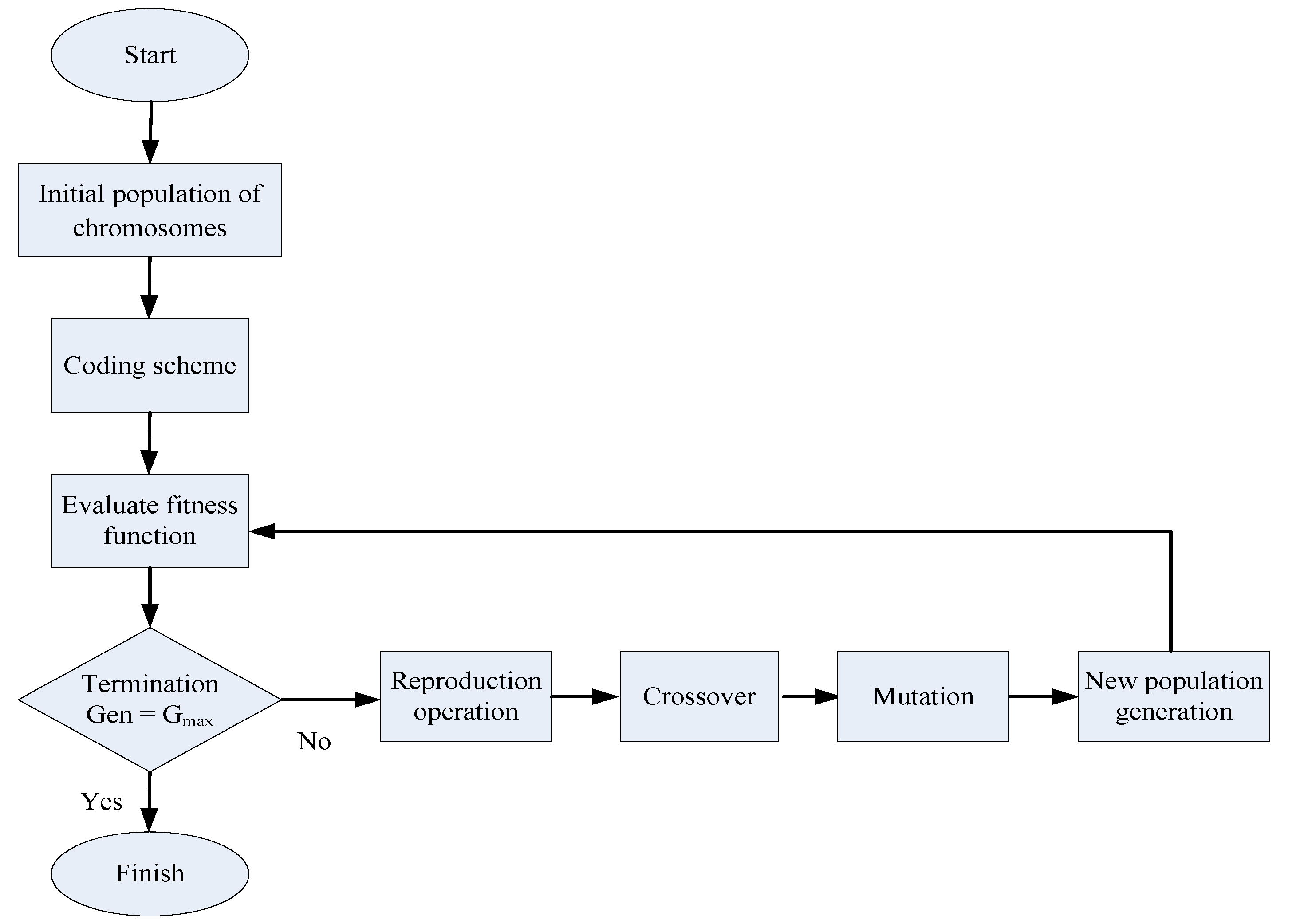
A genetic algorithm can be used to solve the assembly line balancing problem and obtain near-optimal solutions in a short computation time frame. In this study, MATLAB is applied to develop the genetic algorithm model. To prevent a solution being confined in a local optimum and to advance toward the global optimum, both two-cut-point crossover and an inversion mutation operator are applied. The steps of the genetic algorithm are as follows [28,29,30]:
- Step 1.
- Initial population of chromosomes
With a population size of N, the initial population is obtained randomly, and it consists of two types of chromosomes, which are determined randomly.
- Step 2.
- Coding scheme
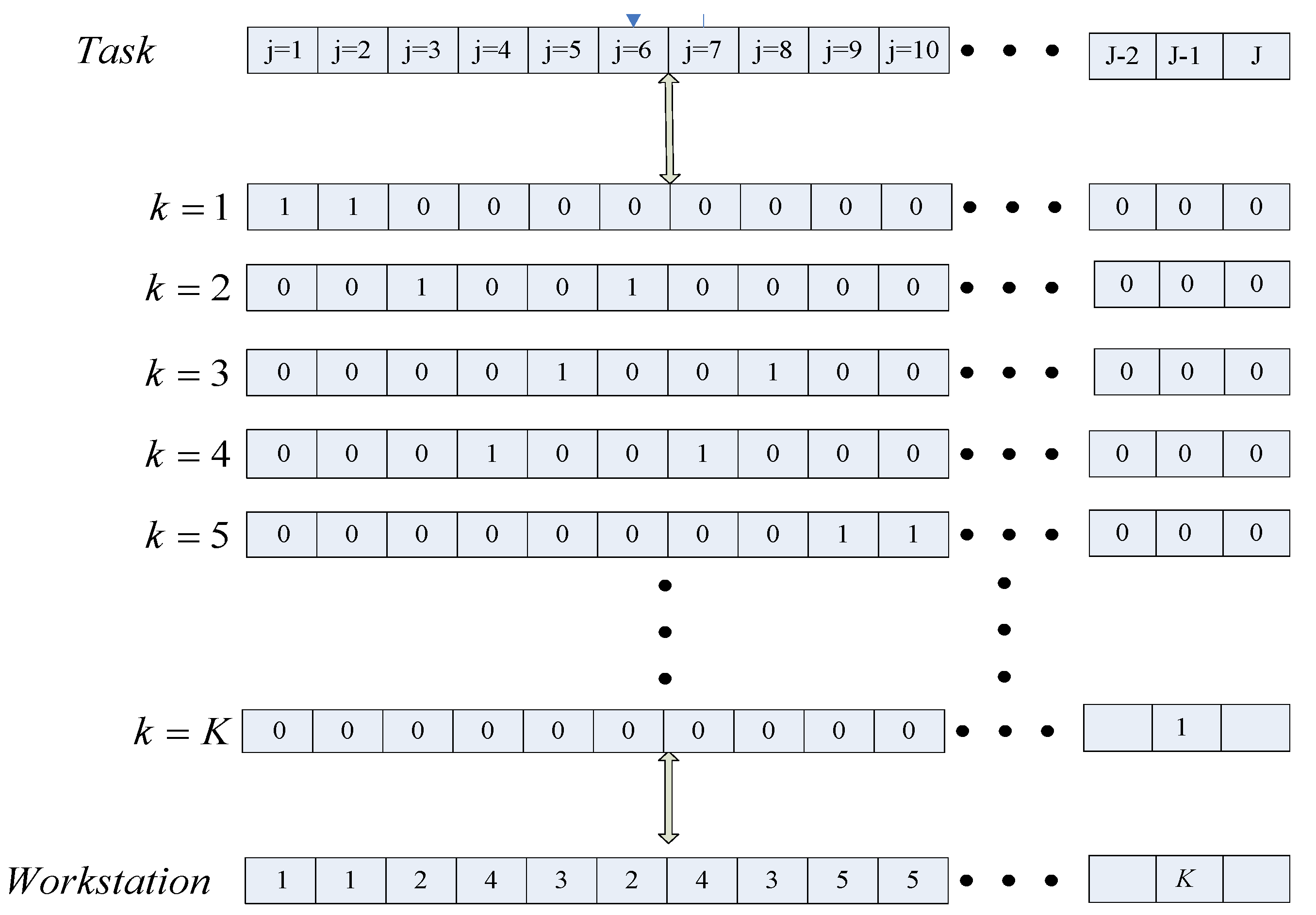
It is assumed that a job can be assigned to one workstation only. The chromosome can be encoded as a string of J binary digits, with the jth gene having a value of 1 if an assignment is made to workstation k and a value of 0 otherwise (see Figure 1). The assignment strategy is:
- Step 3.
- Fitness function evaluation
Define the fitness function for each chromosome as Max λ, where λ is the system satisfaction level. Max λ is the maximum satisfaction level among all the chromosomes across the population.
- Step 4.
- Reproduction operation
Reproduction is controlled by mutation and crossover operators with mutation rate (Pm) and crossover rate (Pc).
- Step 5.
- New population generation
After crossover and mutation operations in a generation, a new population is generated.
- Step 6.
- Termination
The reproduction operation and new population generation are repeated until the objective function is optimized or when the stop criterion is attained. The algorithm is terminated when the generation (Gen) reaches Gmax.
The flowchart of the genetic algorithm process in this research is depicted in Figure 2.
4. Case Studies
4.1. Case Introduction
This study intends to use four objectives to improve the efficiency and benefit of an assembly line. These four objectives may have conflicts among them and may contain uncertainty. Therefore, the proposed mathematical model is applied to solve the problem. A large automobile assembly plant is used as an example for illustration. The basic information of the four cases is shown in Table 1. The number of jobs, maximum number of workstations, planned product cycle time, workstation setup time, and total processing time in each case are different. As the number of jobs increases, the problem becomes more complicated. The complexity increases for later cases.
4.2. Case 1
4.2.1. Single Objective Linear Programming Model
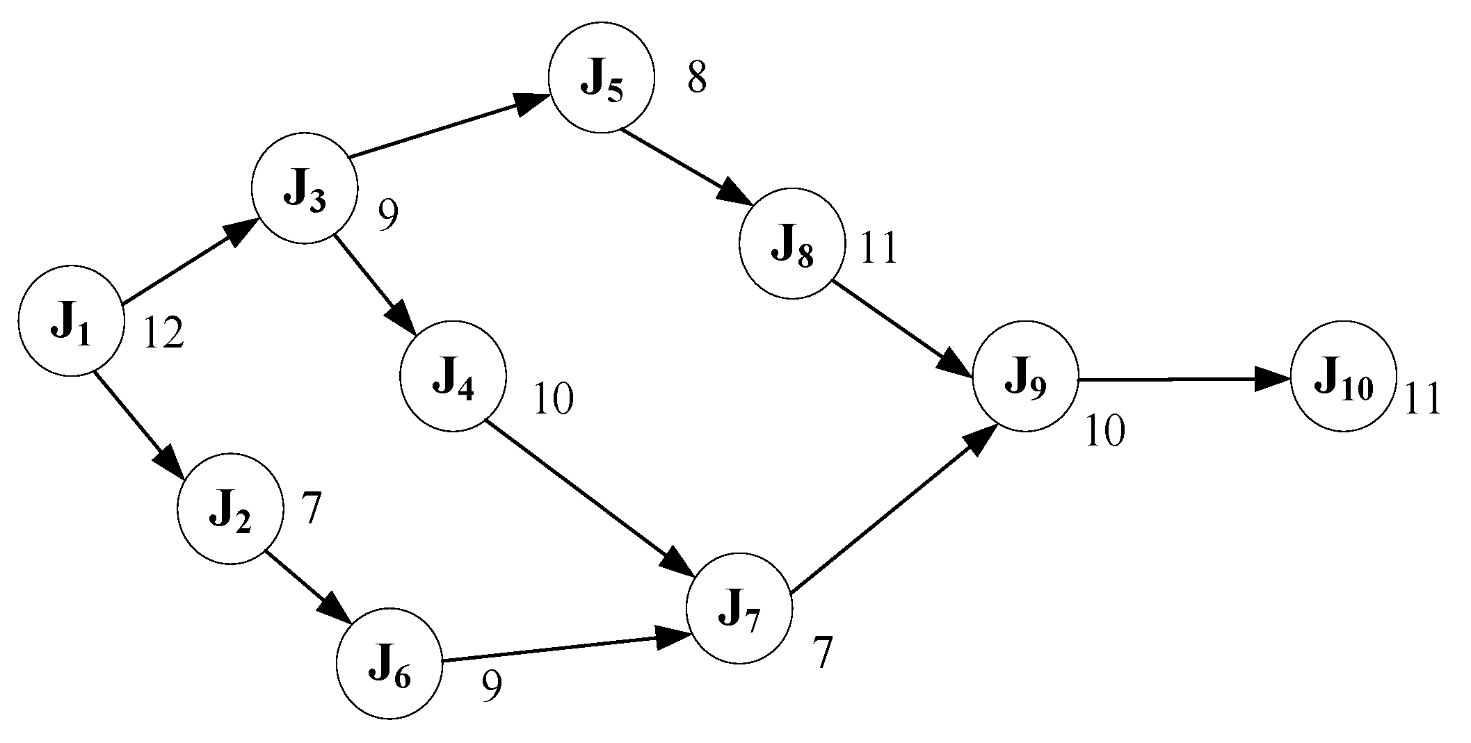
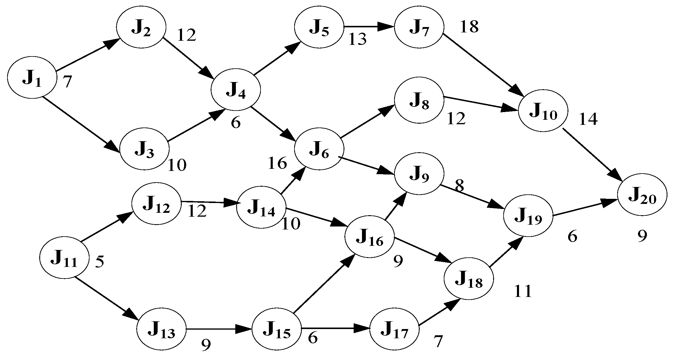
The precedence relationships and processing times of jobs for Case 1 are shown in Figure 3. For instance, job J4 can be processed only after jobs J1 and J3 are completed. Job J3 is a direct predecessor of job J4, and job J1 is an indirect predecessor of job J4. Job J7 can be processed only after jobs J4 and J6 are completed. The total processing time, 94 min, is the summation of the processing times of all jobs. A single objective linear programming model based on each of the four objectives is developed using LINGO 10.
Under the objective of minimizing cycle time (Z1), the results are shown in Table 2 and Table 3. Table 2 shows that to minimize cycle time (Z1), five workstations are required. For example, for the first workstation, jobs A1 and A2 are processed. The setup time is 5 min, and the processing time is:
Processing time = 12 + 7 = 19 (min).
Table 3 shows the performance under each objective while achieving the objective of minimizing cycle time (Z1). For minimizing cycle time (Z1), the decision variable is the cycle time (CT). The cycle time is 26 min, which can be found by summing up the processing time (21 min) and the setup time (5 min) for workstation 5, which has the longest cycle time among all workstations. For minimizing the number of workstations (Z2), the decision variable is the number of workstations (NW), and there are five workstations, as shown in Table 2. For minimizing workload variance (Z3), the decision variable is the workload variance (WV), and 1.76 min is calculated. For minimizing workstation idle time (Z4), the decision variable is the idle time of all workstations (TD), and it is calculated as follows:
TD = (26 − 24) + (26 − 23) + (26 − 24) + (26 − 22) + (26 − 26) = 11 (min).
Under the objective of minimizing number of workstations (Z2), the results are shown in Table 4 and Table 5. Table 4 shows that to minimize the number of workstations (Z2), only one workstation is required to process all jobs. Table 5 shows the performance under each objective while achieving the objective of minimizing number of workstations (Z2). For minimizing cycle time (Z1), the cycle time (CT) is 99 min, which can be found in Table 4. For minimizing number of workstations (NW), there is one workstation, as shown in Table 2. For minimizing workload variance (Z3), the workload variance (WV) is 1569.16 min. For minimizing workstation idle time (Z4), the idle time of all workstations (TD) is 396 min (99*4).
Under the objective of minimizing workload variance (L3), the results are shown in Table 6 and Table 7. Table 6 shows that to minimize workload variance (L3), five workstations are required, and the relevant information about each workstation is listed. Table 7 shows the performance under each objective while achieving the objective of minimizing workload variance (L3). For minimizing cycle time (L1), the cycle time (CT) is 26 min. For minimizing number of workstations (L2), the number of workstations (NW) is 5. For minimizing workload variance (L3), the workload variance (WV) is 26.36 min. For minimizing workstation idle time (L4), the idle time of all workstations (TD) is 11 min.
Under the objective of minimizing workstation idle time (Z4), the results are shown in Table 8 and Table 9. Table 8 shows that to minimize workstation idle time (Z4), five workstations are required, and the relevant information about each workstation is listed. Table 9 shows the performance under each objective while achieving the objective of minimizing workload variance (Z3). Table 10 shows the upper bound, lower bound, deviation, and average of the objective value for the four objectives. The data can be extracted from Table 3, Table 5, Table 7, Table 9. For example, for the first objective, Z1, the decision variable is CT, and the cycle times in Table 3, Table 5, Table 7, Table 9 are 26, 99, 26, and 26, respectively. The highest value is 99, and it is set as the upper bound. The lowest value is 26, and it is set as the lower bound. The deviation and the average are as follows:
Deviation = 99 − 26 = 73,
Average = (99 + 26)/2= 62.5.
4.2.2. Fuzzy Multi-Objective Linear Programming Model
In order to satisfy the four objectives simultaneously, a fuzzy multi-objective linear programming model is constructed based on the concept proposed by Zimmermann [24]. The steps are as follows:
- Step 1.
- Use the results obtained from the single objective linear programming models to set the upper and lower bound for each objective. The fuzzy membership function for cycle time, number of workstations, workload variance, and workstation idle time are , , , and , respectively.
- Step 2.
- Transform the fuzzy multi-objective linear programming model into a single objective linear programming model. The four objectives are transformed into one single objective:
- Step 3.
- Formulate the fuzzy multi-objective linear programming model with satisfaction level λ, as follows:subject to
Objective function (33) is to maximize the satisfaction. Constraint (34) is to minimize the cycle time, CT, where 26 and 99 are the lower bound and upper bound of Z1, respectively. Constraint (35) is to minimize the number of workstations, NW, where 1 and 5 are the lower bound and upper bound of Z2 respectively. Constraint (36) is to minimize the workload variance, WV, where 1.36 and 1413.76 are the lower bound and upper bound of Z3, respectively. Constraint (37) is to minimize the idle time of all workstations, TD, where 11 and 396 are the lower bound and upper bound of Z4, respectively. Constraint (38) sets the satisfaction level to be between 0 and 1. Constraint (39) calculates the total number of workstations used, NW, by summing up all Yk’s, i.e., Y1, Y2, Y3, Y4, and Y5. Constraint (40) calculates the workload variance, WV, based on the differences between Tk and (TP/K). Constraint (41) calculates the total idle time of all workstations, TD. Constraint (42) ensures that the total number of workstations selected for processing must be less than or equal to the maximum number of workstations, that is, 5. Constraints (43)–(47) calculate the completion time of workstation 1 to 5, respectively, by summing up the processing time of all jobs in the specific workstation and the setup time of the specific workstation. Constraint (48) lets cycle time, CT, be the maximum value among the completion times of all workstations, T1,…, T5. Constraints (49)–(53) ensure that the completion time of workstation 1 to 5, respectively, must be less than or equal to the cycle time of the workstation. Constraints (54)–(63) ensure that job A1 to A10, respectively, can only be assigned and processed by one single workstation. Constraints (64)–(74) ensure the sequencing of two of the ten jobs. For instance, Constraint (64) ensures that job A1 must be completed before A2 can go into process in a workstation if they are both processed in the same workstation. Constraint (75) shows that Xjk is a binary variable, which is equal to 1 if job j is processed in workstation k. Constraint (76) shows that Yk is a binary variable, which is equal to 1 if workstation k is selected for processing.
The model contains one variable of λ, one variable of CT, one variable of WV, one variable of TD, one variable of NW, five variables of Tk, five variables of sk, fifty 0-1 variables of Xjk, and five 0-1 variables of Yk. Furthermore, each of Equations (9) and (11) contains five equations. Equation (12) contains ten equations, and Equation (13) contains 11 equations. In this case, the total number of auxiliary variables is 15, the total number of 0-1 variables is 55, and the total number of equations is 40 (9 + 2K + J + Ω).
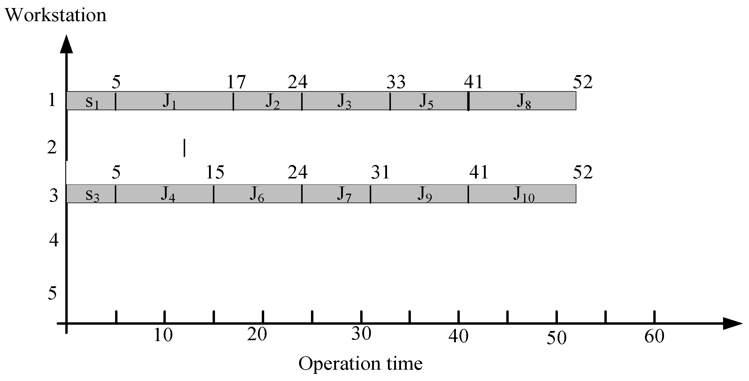
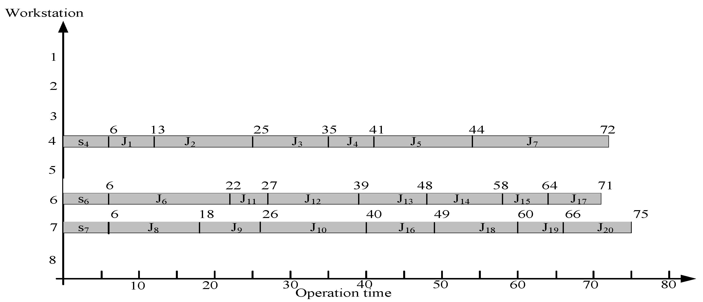
The model can be solved using LINGO 10. The total computation time is 38 s. The results are shown in Table 11 and Table 12. Table 11 shows that two workstations are required, and the relevant information about each workstation is listed. Table 12 shows the objective values and satisfaction levels. For minimizing cycle time (Z1), the cycle time (CT) is 52 min. For minimizing number of workstations (Z2), the number of workstations (NW) is 2. For minimizing workload variance (Z3), the workload variance (WV) is 530.16 min. For minimizing workstation idle time (Z4), the idle time of all workstations (TD) is 141 min. The total satisfaction level λ is 0.63. A Gantt for the solution of Case 1 is depicted in Figure 4.
4.2.3. Genetic Algorithm Model
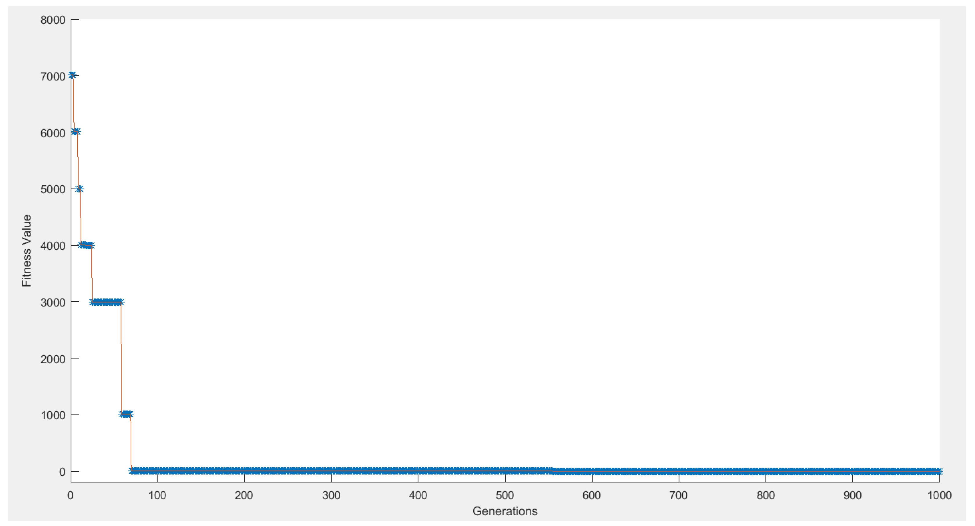
The genetic algorithm model is developed using the software MATLAB. The parameters are set arbitrarily based on past research works and the author’s experiences. The size of the initial population is set as 10. The crossover rate (Pc) is set as 0.99, and this indicates that around 99% pairs of individuals participate in producing offspring. The mutation rate (Pm) is set as 0.01, and this indicates that a gene of a newly created solution is mutated with a probability 0.01. The algorithm is terminated when the 1000th generation is reached. The best generation occurs at the 78th generation, as displayed in Figure 5. The total computation time is 11 s. The solutions generated by the fuzzy multi-objective linear programming model and by the genetic algorithm model are the same, with the total satisfaction level of 0.63.
A design of experiments (DOE) is carried out to examine the genetic algorithm model, and four factors are used: population size (N), crossover rate (Pc), mutation rate (Pm), and maximum generation (Gmax). Table 13 lists the parameters applied to generate the outcomes. With two levels for each factor, a 16 (24) factorial experiment is executed. Since a run has three replicates, 48 trials are performed. The computation time, number of generations, and fitness value of the three trials in a run are applied. Table 14 lists the 16 combinations of the parameters for Case 1. Since the computation time is dependent on maximum generation (Gmax) and population size (N), as Gmax or N increases, the computation time increases. In addition, the number of generations is relatively larger when the population size (N) is smaller. The fitness values in all the 16 runs are the same, i.e., 0.63. This means that the fitness values in all the 16 runs remain stable and consistent. Since the value is the same as that from the fuzzy multi-objective linear programming model with a total satisfaction level λ of 0.63, the optimal solution is obtained.
4.3. Case 2
The precedence relationships and processing times of jobs for Case 2 are shown in Figure 6. A single objective linear programming model based on each of the four objectives is developed using LINGO 10, and Table 15 shows the upper bound, lower bound, deviation, and average of the objective value for the four objectives.
The fuzzy multi-objective linear programming model with satisfaction level λ is constructed and solved using LINGO 10. The total computation time is 342 s. The results are shown in Table 16 and Table 17. Table 16 shows that three workstations are required, and the relevant information about each workstation is listed. Table 17 shows the objective values and satisfaction levels. For minimizing cycle time (L1), the cycle time (CT) is 75 min. For minimizing the number of workstations (L2), the number of workstations (NW) is 3. For minimizing the workload variance (L3), the workload variance (WV) is 1042.75 min. For minimizing the workstation idle time (L4), the idle time of all workstations (TD) is 352 min. The total satisfaction level λ is 0.71. A Gantt for the solution of Case 2 is shown in Figure 7.
Under the genetic algorithm approach, the total computation time is 16 s. The best generation occurs at the 379th generation. The solutions generated by the fuzzy multi-objective linear programming model and by the genetic algorithm model are the same, with the total satisfaction level of 0.71.
4.4. Case 3
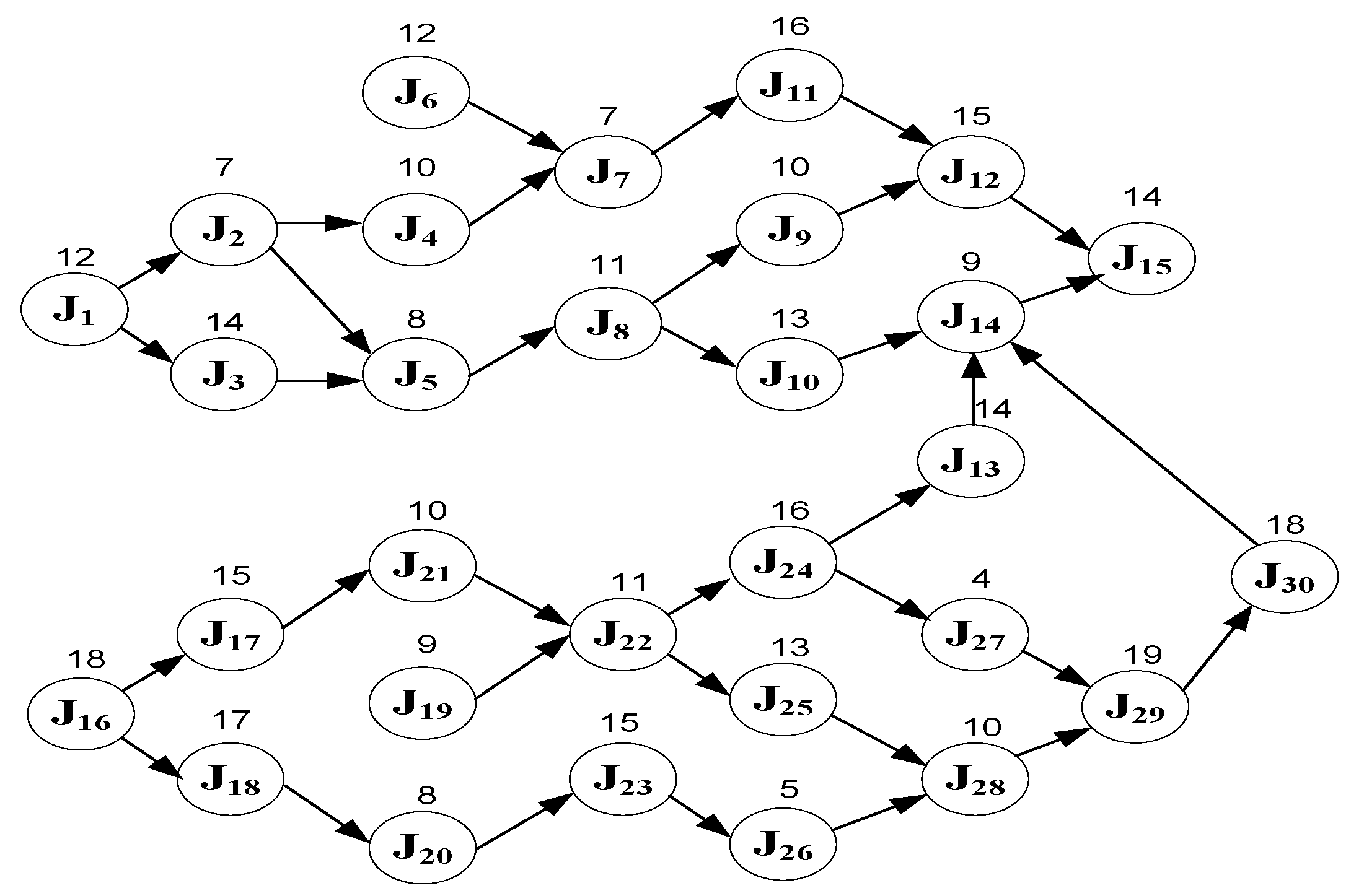
The precedence relationships and processing times of jobs for Case 3 are shown in Figure 8. A single objective linear programming model based on each of the four objectives is constructed, and Table 18 shows the upper bound, lower bound, deviation, and average of the objective value for the four objectives.
The fuzzy multi-objective linear programming model with satisfaction level λ is developed. The model is solved using LINGO 10, and the computation time is 432 s. The results of the model are shown in Table 19 and Table 20. Table 19 shows that three workstations are required, and the relevant information about each workstation is listed. Table 20 shows the objective values and satisfaction levels. For minimizing the cycle time (L1), the cycle time (CT) is 127 min. For minimizing the number of workstations (L2), the number of workstations (NW) is 3. For minimizing the workload variance (L3), the workload variance (WV) is 3024 min. For minimizing the workstation idle time (L4), the idle time of all workstations (TD) is 840 min. The total satisfaction level λ is 0.74.
Under the genetic algorithm approach, the total computation time is 19 s. The best generation occurs at the 718th generation. The solutions generated by the fuzzy multi-objective linear programming model and by the genetic algorithm model are the same, with the total satisfaction level of 0.74.
The calculation time under the fuzzy multi-objective linear programming model is longer than that under the genetic algorithm model. As the complexity of the problem increases, the time required by the fuzzy multi-objective linear programming model increases much more compared with the genetic algorithm model.
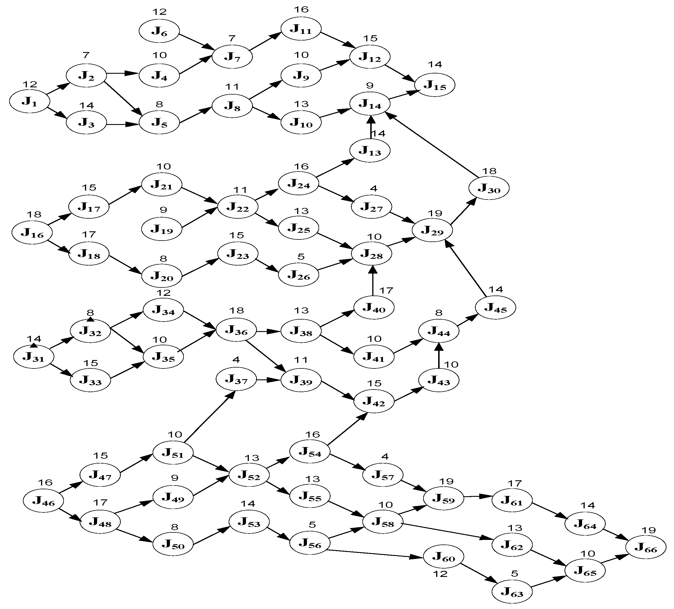
4.5. Case 4
In Case 4, there are 66 jobs, the maximum number of workstations is 12, the planned product cycle time is 1800 min, the workstation setup time is 9 min, and the total processing time is 539 min. The precedence relationships and processing times of jobs for Case 4 are shown in Figure 9. Table 21 shows the upper bound, lower bound, deviation, and average of the objective value for each objective under the single objective linear programming model.
The fuzzy multi-objective linear programming model with satisfaction level λ is developed, and the model is solved using LINGO 10. However, the problem is NP-hard, and it can no longer be solved.
Then, the problem is solved by the genetic algorithm approach. Since the best generation occurs at the 718th generation in Case 3 and the problem becomes much more complicated in Case 4, the algorithm is set to terminate after 2000 generations have elapsed in Case 4. The total computation time is 34 s, and the best generation occurs at the 1156th generation. The solutions generated by the genetic algorithm model are shown in Table 22 and Table 23. Table 22 shows that six workstations are required, and the relevant information about each workstation is listed. Table 23 also shows the objective values and satisfaction levels. For minimizing the cycle time (L1), the cycle time (CT) is 175 min. For minimizing the number of workstations (L2), the number of workstations (NW) is six. For minimizing workload variance (L3), the workload variance (WV) is 5305.25 min. For minimizing workstation idle time (L4), the idle time of all workstations (TD) is 1248 min. The total satisfaction level λ is 0.55.
The calculation under the fuzzy multi-objective linear programming model is no longer probable as the complexity of the problem increases. Although the model cannot be solved by the fuzzy multi-objective linear programming model optimally, the genetic algorithm model can obtain a good solution efficiently.
Five more cases that adopt the dataset of past works are presented in the Appendix A.
5. Discussion
In this study, the satisfaction level λ of the system is the objective function, which is to be maximized. This research considers the ALBP of the automobile manufacturer in a fuzzy environment; several constrained resources are considered as well as the setup times of workstations. The maximin method for the unweighted multiple objectives is adopted. Nine cases are used to examine the proposed fuzzy multi-objective linear programming model and the genetic algorithm model. Since the scales are relatively small for five cases, the fuzzy multi-objective linear programming model can generate optimal solutions, and the genetic algorithm model can also obtain optimal solutions efficiently. The computation time required by the genetic algorithm model under each of the five cases is lower than that required by the fuzzy multi-objective linear programming model. For the other four cases, since the problem scales are larger, the fuzzy multi-objective linear programming model can no longer solve the problem. The genetic algorithm model can still obtain good solutions under a very short computation time. To summarize, the proposed fuzzy multi-objective linear programming model can obtain optimal solutions when the scale of the ALBP is small, and the proposed genetic algorithm model can generate good solutions for large-scale problems efficiently.
The two models proposed in this study are compared with the models developed by Taha et al. [11], Kucukkoc and Zhang [1], and Cerqueus and Delorme [12]. Table 24 shows that among the compared items, the proposed genetic algorithm performed well for nine items, and the proposed fuzzy multi-objective linear programming performed well for 11 items. Thus, the two models are outstanding overall compared to other related models. Since the proposed genetic algorithm model can generate near-optimal solutions within a short computation time, it is suggested to be applied to solve large-scale problems. Even though the proposed models can only solve a one-sided ALBP, they can be tailored to solve a two-sided ALBP, a U-shaped ALBP, or a mixed-model ALBP. This can be our future research direction.
6. Conclusions
In this research, a multi-objective assembly line balancing problem with fuzzy sets and setup time is tackled. A fuzzy multi-objective linear programming model with four objectives, minimizing the cycle time, minimizing the number of workstations, minimizing the workload variance, and minimizing workstation idle time, is constructed first. A genetic algorithm model with a coding scheme for the problem is proposed next. Four case studies are present to examine the two models. The results show that both models can generate optimal solutions when the scale of a problem is not too big. However, when the problem becomes too complicated, the fuzzy multi-objective linear programming model can no longer solve the problem. On the other hand, the genetic algorithm model can obtain near-optimal solutions in a short period of computational time.
There was no work, to the authors’ understanding, that tackled the simple assembly line balancing problems (SALBP) with the consideration of setup time, multiple objectives, and fuzzy sets concurrently. The developed models can reflect a more practical problem in today’s manufacturing environment, for example, when the management wants to consider different performance objectives, or when machine setups are necessary. Companies can enhance customer satisfaction and decrease total cost by applying the models. The outcomes of this research can present important supply chain management information for companies in practice.
For future studies, the initial population of the genetic algorithm could be generated effectively to ensure diversity, for example, by proposing a new approach or adopting the methodology proposed by Taha [11]. In addition, more objectives may be taken into consideration, and different important weights should be given to these objectives. With the fast evolution of technology and manufacturing environment, many new assembly line balancing problems emerge. Novel methodologies and models should be created to solve the problems and help manufacturers achieve a better performance. New metaheuristics methods may be applied or proposed to solve the problems, and a comparison of the methods can be performed.
Author Contributions
Conceptualization, A.H.I.L. and H.-Y.K.; Methodology, A.H.I.L. and H.-Y.K.; Software, H.-Y.K. and C.-L.C.; Validation, A.H.I.L. and C.-L.C.; Formal Analysis, A.H.I.L.; Investigation, H.-Y.K.; Resources, A.H.I.L. and H.-Y.K.; Data Curation, H.-Y.K. and C.-L.C.; Writing—Original Draft Preparation, A.H.I.L. and H.-Y.K.; Writing—Review & Editing, A.H.I.L. and H.-Y.K.; Visualization, H.-Y.K. and C.-L.C.; Supervision, A.H.I.L. and H.-Y.K.; Project Administration, A.H.I.L. and H.-Y.K.; Funding Acquisition, A.H.I.L. and H.-Y.K. All authors have read and agreed to the published version of the manuscript.
Funding
This work was supported in part by the Ministry of Science and Technology in Taiwan under Grant MOST 108-2410-H-167-010.
Institutional Review Board Statement
Not applicable.
Informed Consent Statement
Not applicable.
Data Availability Statement
Not applicable.
Conflicts of Interest
The authors declare no conflict of interest.
Appendix A
The dataset for the benchmarks with 11, 25, 35, 37, and 54 jobs are named cases 5, 6 7, 8, and 9, respectively. The parameters for the five cases are presented in Table A1, and the data for the cases are shown in Table A2, Table A3, Table A4, Table A5 and Table A6. Note that some of the data, such as setup time and the maximum number of workstations, must be made up by the authors because the sample problems do not consider these factors. Table A7, Table A8, Table A9, Table A10 and Table A11 show the objective values and satisfaction levels for Cases 5 to 9, respectively. Table A7 and Table A8 can be obtained by both the fuzzy multi-objective linear programming model and the genetic algorithm model. However, Table A9, Table A10 and Table A11 can only be obtained by the genetic algorithm model.

Table A1.
Parameters for Cases 5–9.
| Sample Problem | Number of Jobs | Maximum Number of Workstations | Workstation Setup Time | Total Processing Time | |
|---|---|---|---|---|---|
| Case 5 | Jackson [31] | 11 | 6 | 5 min | 46 min |
| Case 6 | Rosenberg and Ziegler [32] | 25 | 8 | 6 min | 125 min |
| Case 7 | Gunther et al. [33] | 35 | 10 | 7 min | 484 min |
| Case 8 | Pinarbasi et al. [14] | 37 | 10 | 7 min | 908 min |
| Case 9 | Rashid et al. [19] | 54 | 11 | 9 min | 2864 min |
Table A2.
Data for Case 5.
| Job | Predecessor | Processing Time | Job | Predecessor | Processing Time |
|---|---|---|---|---|---|
| 1 | - | 6 | 7 | 3, 4, 5 | 3 |
| 2 | 1 | 2 | 8 | 6 | 6 |
| 3 | 1 | 5 | 9 | 7 | 5 |
| 4 | 1 | 7 | 10 | 8 | 5 |
| 5 | 1 | 1 | 11 | 9, 10 | 4 |
| 6 | 2 | 2 |
Table A3.
Data for Case 6.
| Job | Predecessor | Processing Time | Job | Predecessor | Processing Time |
|---|---|---|---|---|---|
| 1 | - | 4 | 14 | 13 | 3 |
| 2 | - | 3 | 15 | 12 | 5 |
| 3 | 1, 2 | 9 | 16 | 14 | 3 |
| 4 | 3 | 5 | 17 | 15 | 13 |
| 5 | 4 | 9 | 18 | 16, 17 | 5 |
| 6 | 5 | 4 | 19 | 14 | 2 |
| 7 | 6 | 8 | 20 | 14 | 3 |
| 8 | 4 | 7 | 21 | 20 | 7 |
| 9 | 8 | 5 | 22 | 19, 21 | 5 |
| 10 | 6, 9 | 1 | 23 | 17 | 3 |
| 11 | 7, 8 | 3 | 24 | 21 | 8 |
| 12 | 7 | 1 | 25 | 18, 20, 23 | 4 |
| 13 | 9, 11 | 5 |
Table A4.
Data for Case 7.
| Job | Predecessor | Processing Time | Job | Predecessor | Processing Time |
|---|---|---|---|---|---|
| 1 | - | 29 | 19 | 18 | 19 |
| 2 | 1 | 3 | 20 | 17 | 29 |
| 3 | 2 | 5 | 21 | 16, 20 | 8 |
| 4 | 3 | 22 | 22 | 21 | 10 |
| 5 | 1 | 5 | 23 | 22 | 16 |
| 6 | 5 | 14 | 24 | 23 | 23 |
| 7 | 1, 6 | 2 | 25 | 21 | 5 |
| 8 | 6 | 5 | 26 | 25 | 5 |
| 9 | 8 | 22 | 27 | 24, 26 | 5 |
| 10 | 1 | 30 | 28 | 11, 13, 27 | 40 |
| 11 | 4 | 23 | 29 | 28 | 2 |
| 12 | 1 | 30 | 30 | 21 | 5 |
| 13 | 9 | 23 | 31 | 30 | 5 |
| 14 | 7 | 2 | 32 | 21, 31 | 1 |
| 15 | 14 | 19 | 33 | 11, 13, 27, 32 | 40 |
| 16 | 15 | 29 | 34 | 27 | 2 |
| 17 | - | 2 | 35 | 33 | 2 |
| 18 | 7, 12 | 2 |
Table A5.
Data for Case 8.
| Job | Predecessor | Processing Time | Job | Predecessor | Processing Time |
|---|---|---|---|---|---|
| 1 | - | 23 | 20 | 19 | 13 |
| 2 | - | 12 | 21 | 16 | 14 |
| 3 | 1, 2 | 35 | 22 | 17 | 14 |
| 4 | - | 12 | 23 | - | 12 |
| 5 | 1, 4 | 35 | 24 | 22, 23 | 38 |
| 6 | 3, 5, 8, 10 | 7 | 25 | 21 | 38 |
| 7 | - | 12 | 26 | - | 10 |
| 8 | 1, 7 | 35 | 27 | 26 | 18 |
| 9 | - | 12 | 28 | 24, 25, 27 | 22 |
| 10 | 1, 9 | 35 | 29 | 28 | 15 |
| 11 | 6 | 22 | 30 | 28 | 19 |
| 12 | 6 | 16 | 31 | 17, 18 | 38 |
| 13 | 6 | 54 | 32 | 31 | 43 |
| 14 | 12, 13 | 36 | 33 | 32 | 10 |
| 15 | 6 | 26 | 34 | 11, 14, 15, 20, 29, 30, 33 | 5 |
| 16 | 6 | 42 | 35 | 34 | 20 |
| 17 | 6 | 42 | 36 | 35 | 16 |
| 18 | 6 | 26 | 37 | 36 | 55 |
| 19 | 6 | 26 |
Table A6.
Data for Case 9.
| Job | Predecessor | Processing Time | Job | Predecessor | Processing Time |
|---|---|---|---|---|---|
| 1 | - | 159 | 28 | 26, 27 | 23 |
| 2 | 1 | 16 | 29 | - | 24 |
| 3 | 1 | 29 | 30 | 29 | 46 |
| 4 | 1 | 16 | 31 | 29 | 16 |
| 5 | 1 | 13 | 32 | 29 | 19 |
| 6 | 1 | 20 | 33 | 29 | 75 |
| 7 | 1 | 23 | 34 | 30, 31, 32, 33 | 18 |
| 8 | 1 | 122 | 35 | 3, 4, 5, 6, 10, 19 | 45 |
| 9 | 2, 7 | 112 | 36 | 28, 34 | 151 |
| 10 | 9 | 154 | 37 | 36 | 21 |
| 11 | - | 90 | 38 | 35, 36 | 41 |
| 12 | 11 | 57 | 39 | 36 | 42 |
| 13 | 12 | 12 | 40 | 35, 36 | 40 |
| 14 | 12 | 15 | 41 | 36 | 18 |
| 15 | 8, 13, 14 | 142 | 42 | 35, 36 | 15 |
| 16 | 15 | 87 | 43 | 37, 38, 39, 40, 41, 42 | 41 |
| 17 | 15 | 59 | 44 | 40/41 | 33 |
| 18 | 15 | 23 | 45 | 42 | 38 |
| 19 | 8 | 23 | 46 | 37, 38 | 36 |
| 20 | 16, 17, 18 | 25 | 47 | 37, 38 | 53 |
| 21 | 20 | 49 | 48 | - | 125 |
| 22 | 20 | 24 | 49 | 34, 39 | 92 |
| 23 | 20 | 27 | 50 | 34, 39 | 57 |
| 24 | 20 | 21 | 51 | 34, 39 | 71 |
| 25 | - | 33 | 52 | 34, 39 | 44 |
| 26 | 25 | 61 | 53 | - | 50 |
| 27 | 25 | 76 | 54 | 43, 44, 45, 46, 47, 48, 49, 53 | 142 |
Table A7.
Objective results for Case 5.
| Objective | Objective Value | Objective Function |
|---|---|---|
| Z1 | 23 | = 0.72 |
| Z2 | 2 | = 0.80 |
| Z3 | 117.56 | = 0.64 |
| Z4 | 92 | = 0.68 |
| Total satisfaction level λ = 0.64 | ||
Table A8.
Objective results for Case 6.
| Objective | Objective Value | Objective Function |
|---|---|---|
| Z1 | 30 | = 0.55 |
| Z2 | 5 | = 0.50 |
| Z3 | 114.14 | = 0.55 |
| Z4 | 55 | = 0.55 |
| Total satisfaction level λ = 0.50 | ||
Table A9.
Objective results for Case 7.
| Objective | Objective Value | Objective Function |
|---|---|---|
| Z1 | 162 | = 0.74 |
| Z2 | 3 | = 0.77 |
| Z3 | 5466 | = 0.74 |
| Z4 | 1136 | = 0.74 |
| Total satisfaction level λ = 0.74 | ||
Table A10.
Objective results for Case 8.
| Objective | Objective Value | Objective Function |
|---|---|---|
| Z1 | 304 | = 0.72 |
| Z2 | 3 | = 0.78 |
| Z3 | 19238.56 | = 0.74 |
| Z4 | 2132 | = 0.74 |
| Total satisfaction level λ = 0.72 | ||
Table A11.
Objective results for Case 9.
| Objective | Objective Value | Objective Function |
|---|---|---|
| Z1 | 955 | = 0.71 |
| Z2 | 3 | = 0.80 |
| Z3 | 180771.3 | = 0.74 |
| Z4 | 7641 | = 0.76 |
| Total satisfaction level λ = 0.71 | ||
References
- Kucukkoc, I.; Zhang, D.Z. A mathematical model and genetic algorithm-based approach for parallel two-sided assembly line balancing problem. Prod. Plan. Control. 2015, 26, 874–894. [Google Scholar] [CrossRef] [Green Version]
- Özcan, U.; Toklu, B. Multiple-criteria decision-making in two-sided assembly line balancing: A goal programming and a fuzzy goal programming models. Comput. Oper. Res. 2009, 36, 1955–1965. [Google Scholar] [CrossRef]
- Salveson, M.E. The assembly line balancing problem. J. Ind. Eng. 1955, 6, 18–25. [Google Scholar]
- Erel, E.; Gokcen, H. Shortest-route formulation of mixed-model assembly line balancing problem. Eur. J. Oper. Res. 1999, 116, 194–204. [Google Scholar] [CrossRef] [Green Version]
- Fathi, M.; Fontes, D.B.M.M.; Moris, M.U.; Ghobakhloo, M. Assembly line balancing problem: A comparative evaluation of heuristics and a computational assessment of objectives. J. Model. Manag. 2018, 13, 455–474. [Google Scholar] [CrossRef] [Green Version]
- Baybars, I. A survey of exact algorithms for the simple assembly line balancing problem. Manag. Sci. 1986, 32, 909–932. [Google Scholar] [CrossRef]
- Scholl, A. Balancing and Sequencing Assembly Lines, 2nd ed.; Physica-Verlag: Heidelberg, Germany, 1999. [Google Scholar]
- Becker, C.; Scholl, A. A survey on problems and methods in generalized assembly line balancing. Eur. J. Oper. Res. 2006, 168, 694–715. [Google Scholar] [CrossRef]
- Haq, A.N.; Rengarajan, K.; Jayaprakash, J. A hybrid genetic algorithm approach to mixed-model assembly line balancing. Int. J. Adv. Manuf. Technol. 2005, 28, 337–341. [Google Scholar] [CrossRef]
- Zhang, H.-Y. An improved immune algorithm for simple assembly line balancing problem of type 1. J. Algorithms Comput. Technol. 2017, 11, 317–326. [Google Scholar] [CrossRef]
- Taha, R.B.; El-Kharbotly, A.K.; Sadek, Y.M.; Afia, N.H. A genetic algorithm for solving two-sided assembly line balancing problems. Ain Shams Eng. J. 2011, 2, 227–240. [Google Scholar] [CrossRef] [Green Version]
- Cerqueus, A.; Delorme, X. A branch-and-bound method for the bi-objective simple line assembly balancing problem. Int. J. Prod. Res. 2018, 57, 5640–5659. [Google Scholar] [CrossRef]
- Ritt, M.; Costa, A.M. Improved integer programming models for simple assembly line balancing and related problems. Int. Trans. Oper. Res. 2015, 25, 1345–1359. [Google Scholar] [CrossRef] [Green Version]
- Pinarbasi, M.; Alakas, H.M.; Yuzukirmizi, M. A constraint programming approach to type-2 assembly line balancing problem with assignment restrictions. Assem. Autom. 2019, 39, 813–826. [Google Scholar] [CrossRef]
- Mardani-Fard, H.A.; Hadi-Vencheh, A.; Mahmoodirad, A.; Niroomand, S. An effective hybrid goal programming approach for multi-objective straight assembly line balancing problem with stochastic parameters. Oper. Res. 2018, 20, 1939–1976. [Google Scholar] [CrossRef]
- Abu Bakar, N.; Ramli, M.F.; Zakaria, M.Z.; Sin, T.C.; Masran, H. Solving assembly line balancing problem using heuristic: A case study of power transformer in electrical industry. Indones. J. Electr. Eng. Comput. Sci. 2020, 17, 850–857. [Google Scholar] [CrossRef] [Green Version]
- Li, Z.; Kucukkoc, I.; Tang, Q. A comparative study of exact methods for the simple assembly line balancing problem. Soft Comput. 2020, 24, 11459–11475. [Google Scholar] [CrossRef]
- Li, Z.; Janardhanan, M.N.; Tang, Q. Multi-objective migrating bird optimization algorithm for cost-oriented assembly line balancing problem with collaborative robots. Neural Comput. Appl. 2021, 1–22. [Google Scholar] [CrossRef]
- Rashid, M.F.F.A.; Rose, A.N.M.; Mohamed, N.M.Z.N.; Romlay, F.R.M. Improved moth flame optimization algorithm to op-timize cost-oriented two-sided assembly line balancing. Eng. Comput. 2020, 37, 638–663. [Google Scholar] [CrossRef]
- Kim, Y.K.; Kim, Y.; Kim, Y.J. Two-sided assembly line balancing: A genetic algorithm approach. Prod. Plan. Control. 2000, 11, 44–53. [Google Scholar] [CrossRef]
- Kim, Y.K.; Song, W.S.; Kim, J.H. A mathematical model and a genetic algorithm for two-sided assembly line balancing. Comput. Oper. Res. 2009, 36, 853–865. [Google Scholar] [CrossRef]
- Tanhaie, F.; Rabbani, M.; Manavizadeh, N. Simultaneous balancing and worker assignment problem for mixed-model as-sembly lines in a make-to-order environment considering control points and assignment restrictions. J. Model. Manag. 2020, 15, 1–34. [Google Scholar] [CrossRef]
- Eslamipoor, R.; Nobari, A. A mathematical model for an integrated assembly line regarding learning and fatigue effects. Robotica 2021, 1–17. [Google Scholar] [CrossRef]
- Zimmermann, H.-J. Fuzzy programming and linear programming with several objective functions. Fuzzy Sets Syst. 1978, 1, 45–55. [Google Scholar] [CrossRef]
- Zwick, R.; Zimmermann, H.-J. Fuzzy set theory and its applications. Am. J. Psychol. 1993, 106, 304. [Google Scholar] [CrossRef]
- Ghaffar, A.R.A.; Hasan, G.; Ashraf, Z.; Khan, M.F. Fuzzy goal programming with an imprecise intuitionistic fuzzy preference relations. Symmetry 2020, 12, 1548. [Google Scholar] [CrossRef]
- Kang, H.-Y.; Lee, A.H. Inventory replenishment model using fuzzy multiple objective programming: A case study of a high-tech company in Taiwan. Appl. Soft Comput. 2010, 10, 1108–1118. [Google Scholar] [CrossRef]
- Qi, J.G.; Burns, G.R.; Harrison, D.K. The application of parallel multipopulation genetic algorithms to dynamic job-shop scheduling. Int. J. Adv. Manuf. Technol. 2000, 16, 609–615. [Google Scholar] [CrossRef]
- Lee, A.H.I.; Kang, H.-Y.; Lai, C.-M. Solving lot-sizing problem with quantity discount and transportation cost. Int. J. Syst. Sci. 2013, 44, 760–774. [Google Scholar] [CrossRef]
- Kang, H.-Y.; Pearn, W.L.; Chung, I.-P.; Lee, A.H.I. An enhanced model for the integrated production and transportation problem in a multiple vehicles environment. Soft Comput. 2015, 20, 1415–1435. [Google Scholar] [CrossRef]
- Jackson, J.R. An extension of Johnson’s results on job IDT scheduling. Nav. Res. Logist. Q. 1956, 3, 201–203. [Google Scholar] [CrossRef]
- Rosenberg, O.; Ziegler, H. A comparison of heuristic algorithms for cost-oriented assembly line balancing. Math. Methods Oper. Res. 1992, 36, 477–495. [Google Scholar] [CrossRef]
- E Gunther, R.; Johnson, G.D.; Peterson, R.S.; Günther, R. Currently practiced formulations for the assembly line balance problem. J. Oper. Manag. 1983, 3, 209–221. [Google Scholar] [CrossRef]
Figure 1.
Chromosome of coding scheme and workstation assignment.

Figure 2.
Graphical representation of genetic algorithm process.

Figure 3.
Precedence relationships and processing times of jobs for Case 1.

Figure 4.
Gantt chart for the solution of Case 1.

Figure 5.
The convergence of the genetic algorithm approach for Case 1.

Figure 6.
Precedence relationships and processing times of jobs for Case 2.

Figure 7.
Gantt chart for the solution of Case 2.

Figure 8.
Precedence relationships and processing times of jobs for Case 3.

Figure 9.
Precedence relationships and processing times of jobs for Case 4.

Table 1.
Parameters for the cases.
| Number of Jobs | Maximum Number of Workstations | Workstation Setup Time | Total Processing Time | |
|---|---|---|---|---|
| Case 1 | 10 | 5 | 5 min | 94 min |
| Case 2 | 20 | 8 | 6 min | 200 min |
| Case 3 | 30 | 10 | 7 min | 360 min |
| Case 4 | 66 | 12 | 9 min | 539 min |
Table 2.
Workstation results under the objective Z1 for Case 1.
| Workstation | Processing Time | Setup Time | Cycle Time | Jobs |
|---|---|---|---|---|
| 1 | 19 | 5 | 24 | J1, J2 |
| 2 | 18 | 5 | 23 | J3, J6 |
| 3 | 19 | 5 | 24 | J5, J8 |
| 4 | 17 | 5 | 22 | J4, J7 |
| 5 | 21 | 5 | 26 | J9, J10 |
Table 3.
Objective results under the objective Z1 for Case 1.
| Objective | Decision Variable | Objective Value |
|---|---|---|
| Z1 | CT | 26 |
| Z2 | NW | 5 |
| Z3 | WV | 1.76 |
| Z4 | TD | 11 |
Table 4.
Workstation results under the objective Z2 for Case 1.
| Workstation | Processing Time | Setup Time | Cycle Time | Jobs |
|---|---|---|---|---|
| 1 | 0 | 0 | 0 | |
| 2 | 0 | 0 | 0 | |
| 3 | 0 | 0 | 0 | |
| 4 | 0 | 0 | 0 | |
| 5 | 94 | 5 | 99 | J1, J2, J3, J4, J5, J6, J7, J8, J9, J10 |
Table 5.
Objective results under the objective Z2 for Case 1.
| Objective | Decision Variable | Objective Value |
|---|---|---|
| Z1 | CT | 99 |
| Z2 | NW | 1 |
| Z3 | WV | 1413.76 |
| Z4 | TD | 396 |
Table 6.
Workstation results under the objective Z3 for Case 1.
| Workstation | Processing Time | Setup Time | Cycle Time | Jobs |
|---|---|---|---|---|
| 1 | 19 | 5 | 24 | A1, A2 |
| 2 | 18 | 5 | 23 | A3, A6 |
| 3 | 18 | 5 | 23 | A4, A5 |
| 4 | 18 | 5 | 23 | A7, A8 |
| 5 | 21 | 5 | 26 | A9, A10 |
Table 7.
Objective results under the objective Z3 for Case 1.
| Objective | Decision Variable | Objective Value |
|---|---|---|
| Z1 | CT | 26 |
| Z2 | NW | 5 |
| Z3 | WV | 1.36 |
| Z4 | TD | 11 |
Table 8.
Workstation results under the objective Z4 for Case 1.
| Workstation | Processing Time | Setup Time | Cycle Time | Jobs |
|---|---|---|---|---|
| 1 | 21 | 5 | 26 | J1, J3 |
| 2 | 17 | 5 | 22 | J2, J4 |
| 3 | 16 | 5 | 21 | J6, J7 |
| 4 | 19 | 5 | 24 | J5, J8 |
| 5 | 21 | 5 | 26 | J9, J10 |
Table 9.
Objective results under the objective Z4 for Case 1.
| Objective | Decision Variable | Objective Value |
|---|---|---|
| Z1 | CT | 26 |
| Z2 | NW | 5 |
| Z3 | WV | 4.16 |
| Z4 | TD | 11 |
Table 10.
Bounds for each objective for Case 1.
| Decision Variable | Upper Bound | Lower Bound | Deviation | Average |
|---|---|---|---|---|
| CT | 99 | 26 | 73 | 62.5 |
| NW | 5 | 1 | 4 | 3 |
| WV | 1413.76 | 1.36 | 1412.4 | 707.56 |
| TD | 396 | 11 | 385 | 203.5 |
Table 11.
Workstation results under fuzzy multi-objective linear programming for Case 1.
| Workstation | Processing Time | Setup Time | Cycle Time | Jobs |
|---|---|---|---|---|
| 1 | 47 | 5 | 52 | J1, J2, J3, J5, J8 |
| 2 | ||||
| 3 | 47 | 5 | 52 | J4, J6, J7, J9, J10 |
| 4 | ||||
| 5 |
Table 12.
Objective results under fuzzy multi-objective linear programming for Case 1.
| Objective | Objective Value | Objective Function |
|---|---|---|
| Z1 | 52 | = 0.64 |
| Z2 | 2 | = 0.75 |
| Z3 | 530.16 | = 0.63 |
| Z4 | 141 | = 0.66 |
| Total satisfaction level λ = 0.63 | ||
Table 13.
The parameters of the genetic algorithm.
| N | Pc | Pm | Gmax |
|---|---|---|---|
| 10 | 0.9 | 0.01 | 1000 |
| 50 | 0.99 | 0.05 | 2000 |
Table 14.
The 16 combinations of the parameters for Case 1.
| Run | N | Pc | Pm | Gmax | Computation Time | Number of Generations | Fitness Value |
|---|---|---|---|---|---|---|---|
| 1 | 10 | 0.9 | 0.01 | 1000 | 11 | 79 | 0.63 |
| 2 | 10 | 0.9 | 0.01 | 2000 | 19 | 61 | 0.63 |
| 3 | 10 | 0.9 | 0.05 | 1000 | 11 | 57 | 0.63 |
| 4 | 10 | 0.9 | 0.05 | 2000 | 19 | 68 | 0.63 |
| 5 | 10 | 0.99 | 0.01 | 1000 | 11 | 77 | 0.63 |
| 6 | 10 | 0.99 | 0.01 | 2000 | 19 | 85 | 0.63 |
| 7 | 10 | 0.99 | 0.05 | 1000 | 11 | 167 | 0.63 |
| 8 | 10 | 0.99 | 0.05 | 2000 | 19 | 132 | 0.63 |
| 9 | 50 | 0.9 | 0.01 | 1000 | 39 | 92 | 0.63 |
| 10 | 50 | 0.9 | 0.01 | 2000 | 74 | 65 | 0.63 |
| 11 | 50 | 0.9 | 0.05 | 1000 | 38 | 93 | 0.63 |
| 12 | 50 | 0.9 | 0.05 | 2000 | 73 | 91 | 0.63 |
| 13 | 50 | 0.99 | 0.01 | 1000 | 38 | 85 | 0.63 |
| 14 | 50 | 0.99 | 0.01 | 2000 | 74 | 67 | 0.63 |
| 15 | 50 | 0.99 | 0.05 | 1000 | 39 | 55 | 0.63 |
| 16 | 50 | 0.99 | 0.05 | 2000 | 75 | 48 | 0.63 |
Table 15.
Bounds for each objective for Case 2.
| Decision Variable | Upper Bound | Lower Bound | Deviation | Average |
|---|---|---|---|---|
| CT | 206 | 32 | 174 | 119 |
| NW | 8 | 1 | 7 | 4.5 |
| WV | 4642 | 8.75 | 4633.25 | 2325.375 |
| TD | 1400 | 8 | 1392 | 704 |
Table 16.
Workstation results under fuzzy multi-objective linear programming for Case 2.
| Workstation | Processing Time | Setup Time | Cycle Time | Jobs |
|---|---|---|---|---|
| 1 | ||||
| 2 | ||||
| 3 | ||||
| 4 | 66 | 6 | 72 | A1, A2, A3, A4, A5, A7 |
| 5 | ||||
| 6 | 65 | 6 | 71 | A6, B1, B2, B3, B4, B5, B7 |
| 7 | 69 | 6 | 75 | A8, A9, A10, B6, B8, B9, B10 |
| 8 |
Table 17.
Objective results under fuzzy multi-objective linear programming for Case 2.
| Objective | Objective Value | Objective Function |
|---|---|---|
| Z1 | 75 | = 0.75 |
| Z2 | 3 | = 0.71 |
| Z3 | 1042.75 | = 0.78 |
| Z4 | 352 | = 0.75 |
| Total satisfaction level λ = 0.71 | ||
Table 18.
Bounds for each objective for Case 3.
| Decision Variable | Upper Bound | Lower Bound | Deviation | Average |
|---|---|---|---|---|
| CT | 367 | 43 | 323 | 205 |
| NW | 10 | 1 | 9 | 5.5 |
| WV | 11664 | 0.7 | 11663.3 | 5832.35 |
| TD | 3240 | 1.8 | 3238.2 | 1620.9 |
Table 19.
Workstation results under fuzzy multi-objective linear programming for Case 3.
| Workstation | Processing Time | Setup Time | Cycle Time | Jobs |
|---|---|---|---|---|
| 1 | 120 | 7 | 127 | J1, J2, J4, J6, J7, J16, J18, J20, J21, J23, J26 |
| 2 | ||||
| 3 | 120 | 7 | 127 | J3, J5, J17, J19, J24, J25, J27, J28 |
| 4 | ||||
| 5 | ||||
| 6 | ||||
| 7 | ||||
| 8 | 120 | 7 | 127 | J8, J9, J10, J11, J12, J13, J14, J15, J22, J29, J30 |
| 9 | ||||
| 10 |
Table 20.
Objective results under fuzzy multi-objective linear programming for Case 3.
| Objective | Objective Value | Objective Function |
|---|---|---|
| Z1 | 127 | = 0.74 |
| Z2 | 3 | = 0.78 |
| Z3 | 3024 | = 0.74 |
| Z4 | 840 | = 0.74 |
| Total satisfaction level λ = 0.74 | ||
Table 21.
Bounds for each objective for Case 4.
| Decision Variable | Upper Bound | Lower Bound | Deviation | Average |
|---|---|---|---|---|
| CT | 807 | 75 | 732 | 441 |
| NW | 12 | 1 | 11 | 6.5 |
| WV | 49,749 | 7 | 49,742 | 24,878 |
| TD | 8877 | 12 | 8865 | 4444.5 |
Table 22.
Workstation results under the genetic algorithm model for Case 4.
| Workstation | Processing Time | Setup Time | Cycle Time | Jobs |
|---|---|---|---|---|
| 1 | 100 | 9 | 109 | J1, J2, J3, J4, J5, J6, J7, J8, J9, J21 |
| 2 | 140 | 9 | 149 | J46, J47, J48, J49, J50, J51, J52, J53, J54, J55, J56, J57 |
| 3 | 152 | 9 | 161 | J11, J12, J31, J32, J33, J34, J35, J36, J37, J38, J40, J41 |
| 4 | 121 | 9 | 130 | J10, J16, J17, J18, J19, J20, J22, J24, J25 |
| 5 | 166 | 9 | 175 | J13, J14, J15, J23, J26, J27, J28, J29, J30, J39, J42, J43, J44, J45 |
| 6 | 119 | 9 | 128 | J58, J59, J60, J61, J62, J63, J64, J65, J66 |
| 7 | ||||
| 8 | ||||
| 9 | ||||
| 10 | ||||
| 11 | ||||
| 12 |
Table 23.
Objective results under the genetic algorithm model for Case 4.
| Objective | Objective Value | Objective Function |
|---|---|---|
| Z1 | 175 | = 0.86 |
| Z2 | 6 | = 0.55 |
| Z3 | 5305.25 | = 0.89 |
| Z4 | 1248 | = 0.86 |
| Total satisfaction level .55 | ||
Table 24.
Comparisons among related works.
| Compared Items | Taha et al. [11] | Kucukkoc and Zhang [1] | Cerqueus and Delorme [12] | Proposed Genetic Algorithm | Proposed Fuzzy Multi-Objective Linear Programming |
|---|---|---|---|---|---|
| Algorithm | Genetic algorithm | Genetic algorithm | Branch-and-bound search | Genetic algorithm | Exact |
| Accuracy | Near optimal | Near optimal | Near optimal | Near optimal | Optimal |
| One-sided ALBP | Yes | Yes | Yes | Yes | Yes |
| Two-sided ALBP | Yes | Yes | No | No | No |
| Multiple objectives | No | No | Yes | Yes | Yes |
| Cycle time | Yes | Yes | Yes | Yes | Yes |
| Number of workstations | No | Yes | Yes | Yes | Yes |
| Workload variance | No | No | No | Yes | Yes |
| Idle time | No | No | Yes | Yes | Yes |
| Setup time | No | No | No | Yes | Yes |
| Fuzzy sets | No | No | No | Yes | Yes |
| Solved by common software packages | No | No | No | No | Yes |
| Solve binary behavior | Yes | Yes | Yes | Yes | Yes |
Publisher’s Note: MDPI stays neutral with regard to jurisdictional claims in published maps and institutional affiliations. |
© 2021 by the authors. Licensee MDPI, Basel, Switzerland. This article is an open access article distributed under the terms and conditions of the Creative Commons Attribution (CC BY) license (http://creativecommons.org/licenses/by/4.0/).
Share and Cite
MDPI and ACS Style
Lee, A.H.I.; Kang, H.-Y.; Chen, C.-L. Multi-Objective Assembly Line Balancing Problem with Setup Times Using Fuzzy Goal Programming and Genetic Algorithm. Symmetry 2021, 13, 333. https://doi.org/10.3390/sym13020333
AMA Style
Lee AHI, Kang H-Y, Chen C-L. Multi-Objective Assembly Line Balancing Problem with Setup Times Using Fuzzy Goal Programming and Genetic Algorithm. Symmetry. 2021; 13(2):333. https://doi.org/10.3390/sym13020333
Chicago/Turabian StyleLee, Amy H. I., He-Yau Kang, and Chong-Lin Chen. 2021. "Multi-Objective Assembly Line Balancing Problem with Setup Times Using Fuzzy Goal Programming and Genetic Algorithm" Symmetry 13, no. 2: 333. https://doi.org/10.3390/sym13020333
Note that from the first issue of 2016, this journal uses article numbers instead of page numbers. See further details here.