
Flavour Anomalies in a U(1) SUSY Extension of the SM


1
Joint Institute for Nuclear Research, 141980 Dubna, Russia
2
P.N. Lebedev Physical Institute of the Russian Academy of Sciences, 119991 Moscow, Russia
*
Author to whom correspondence should be addressed.
Symmetry 2021, 13(2), 191; https://doi.org/10.3390/sym13020191
Submission received: 11 January 2021
/
Revised: 20 January 2021
/
Accepted: 21 January 2021
/
Published: 26 January 2021
(This article belongs to the Special Issue Symmetry in Particle Physics II)
Abstract
:Flavour anomalies have attracted a lot of attention over recent years as they provide unique hints for possible New Physics. Here, we consider a supersymmetric (SUSY) extension of the Standard Model (SM) with an additional anomaly-free gauge group. The key feature of our model is the particular choice of non-universal charges to the gauge boson , which not only allows a relaxation of the flavour discrepancies but, contrary to previous studies, can reproduce the SM mixing matrices both in the quark and lepton sectors. We pay special attention to the latter and explicitly enumerate all parameters relevant for our calculation in the low-energy effective theory. We find regions in the parameter space that satisfy experimental constraints on meson mixing and LHC searches and can alleviate the flavour anomalies. In addition, we also discuss the predictions for lepton-flavour violating decays and .
1. Introduction
The Standard Model (SM) is a very successful theory, explaining most experimental results. However, there are experimental discrepancies with some of the SM predictions. Among interesting processes there are those that receive special attention in the literature. Most of them are Flavour-Changing-Neutral-Current (FCNC) transitions that in the SM are loop-suppressed and have enhanced sensitivity to the New Physics (NP) effect. The role of such kind of observable is two-fold. After being measured compatible with the SM, it poses severe constraints on the Beyond-the-SM (BSM) scenarios. On the other hand, if there is a tension between the SM and experiment, it stimulates various speculations on possible solutions in the context of BSM models.
In particular, one usually discusses the transitions. The LHCb Collaboration has made measurements of [1] that deviate from the SM predictions [2]. The Belle Collaboration finds similar results [3]. The main discrepancy is in the angular observable [4], averaged over the invariant mass of the lepton pair in the ranges and . Recent LHCb measurement [5]
reports the significance of deviation to be and , respectively (the significance of the discrepancy depends on the assumptions about the theoretical hadronic uncertainties [6]).
Other important observables are ratios [7,8,9] in the dilepton invariant mass-squared range
that test lepton flavour non-universality (see also [10]). They also deviate from the SM predictions of and . Even though the most recent data seems to be consistent with the SM at 2.5 [9], or has large error bars [11], the and puzzles still provide very intriguing insights on possible NP.
Finally, let us mention constraints from the meson-mixing. The mass difference of the neutral meson system, , provides a severe constraint for any NP model aiming at an explanation of the B-physics anomalies. For quite some time the SM value for was in perfect agreement with experimental results, see e.g., [12]. Taking however, the most recent lattice inputs, in particular the new average provided by the Flavour Lattice Averaging Group (FLAG) one gets a SM value ps [13] considerably above the measurement [14]
One can also consider the constraints due to the mixing in the meson system. For example, for the dimensionless ratio of the mass difference over the averaged decay width (see, e.g., reference [14,15])) we have (under assumption that there is no CP-violation)
The uncertainties of SM prediction is rather large and as SM value we take a rough estimate provided by Flavio (2.0.0) package [16] .
It is interesting that all the observables for , , and can be explained by the weak effective theory (WET) with a Hamiltonian of the form (see, e.g., references [16,17]),
where relevant operators are ()
for the transitions, and
together with
for the above-mentioned meson mixing. For further convenience we also list here the operators that give rise to lepton-flavour violating decays of B mesons, which were studied experimentally by BaBar Collaboration [18,19]:
The analyses before Moriond 2019 [17] and after Moriond 2019 [20] show that several patterns of NP contributions explain the discrepancies significantly better than the SM. In all cases, there should be a sizable negative contribution to .
A way to address the anomalies is to introduce a gauge boson which couples to muons and down-type quarks. For instance, gauge symmetry is employed to control the flavor dependent couplings of the boson [21]. It is shown in [22] that anomalies can be successfully explained in models with a boson.
In this work, we consider a non-universal gauge extension of the Minimal Supersymmetric Standard Model (MSSM), with family dependent couplings to quarks and leptons [23,24]. Such an could emerge in GUT, superstring constructions or dynamical electroweak breaking theories. We take this extended supersymmetric model as a simple extension of MSSM, allowing more flexibility in model parameters.
We analyse this model in the context of all three SM fermion families. This allows us to explicitly discuss both the Cabibbo-Kobayashi-Maskawa (CKM) and Pontecorvo–Maki–Nakagawa–Sakata (PMNS) matrices together with additional mixing allowed in the model. The purpose of this paper is to demonstrate the existence of scenarios that can relax the tension in flavour anomalies and discuss some interesting manifestations of the model. A more detailed analysis of the expected phenomenology in a wider parameter space is delegated to future work.
2. Model Description
Let us briefly describe our model and set up the notation. We consider a extension of the MSSM similar to that of reference [24]. In addition to the chiral multiplets of the MSSM, we also introduce a singlet (strictly speaking, the field S is singlet only w.r.t. the SM gauge group) superfield S, which allows one to break spontaneously and generate mass for the corresponding boson. To account for the massive neutrinos three right-handed chiral superfields are also introduced.
The charges of the additional gauge group are not universal and, thus, potentially allow one to accommodate for the flavour anomalies discussed in the literature. As usual, the requirement that there should be no gauge anomalies in the model, imposes important restrictions on the charges. While in the non-supersymmetric extensions one usually takes into account only the SM fermions (see, e.g., [25,26]), with SUSY we have plenty of half-spin superpartners, which can also contribute to the gauge anomalies.
It is known that models with charge assignments and , where () are baryon (lepton) numbers of the i generations are free from anomalies. Due to this, in reference [24] the model based on with and was considered. A key observation of reference [24] was the fact that the Higgs superfield and the chiral lepton superfields have the same SM charges, so one can, e.g., switch the charges of and without spoiling the anomaly cancellation. As a consequence, the contribution of the left-handed (LH) taus to the anomalies is replaced by that of higgsinos. Moreover, since the right-handed (RH) neutrinos also carry the corresponding lepton numbers, we can switch the charges of and S.
Our initial motivation was to extend the study of reference [24] and analyse the effect of a more general mixing in both the quark and lepton sectors. However, one can show that the lepton mass matrices compatible with charges of [24] turn out to be block-diagonal. Due to this, one has unbroken global symmetry corresponding to the lepton number and can not accommodate for the PMNS mixing in the neutrino sector. Parameter counting based on broken flavour symmetries confirms this statement.
To circumvent this problem we modify the initial charge assignment to allow more general Yukawa textures in the lepton sector. We started with and made the substitutions , . Among possible solutions we have chosen the one with , , :
where () assigns (1) to the top-quark (i generation lepton) superfields (both LH and RH (we use LH charge-conjugated superfields to account for the RH particles, so in (11) one can write ), while , S and are equal to one for the higgs , the singlet S and the right-handed tau superfields, respectively, and zero otherwise. The quantum numbers corresponding to (11) can be found in Table 1.
One can see that (modulo , which can be absorbed into redefinition of ) in the quark sector we have the same charges as in reference [24]. However, the charges of , S and are flipped. In addition, the fields carrying are also coupled to . The corresponding R-parity conserving superpotential is given by
where LH chiral quark (lepton) superfields are denoted by (), and , , , and correspond to up-quark, down-quark, charged-lepton and neutrino RH fields, respectively. Since is not charged we also add a Majorana mass . The two higgs superfields and are coupled to the singlet S, the vacuum expectation value (VEV) of which gives rise to the effective parameter and provide a solution to the problem.
The gauge field couples to quarks and leptons as
Here corresponds to the gauge coupling and all fermions are written in the weak basis. In what follows we assume that the mixing is negligible [24]. The pattern (13) allows one to evade the constraints on the production cross-section from the LHC dilepton searches (see, e.g., reference [27]). The weak eigenstates in Equation (13) have to be rewritten in terms of mass eigenstates, which originate from the diagonalization of the mass matrices. The latter are related by spontaneous symmetry breaking to the (effective) Yukawa couplings. However, one can see that certain Yukawa interactions are not allowed at the tree level. Nevertheless, it is possible to consider the non-holomorphic soft SUSY-breaking terms [28]
which are not forbidden by the gauge symmetry and in which scalar superpartners of the SM fermions couple to the “wrong” Higgs doublets. Given (14), additional contribution to the fermion mass matrices are generated [28], which similar to reference [24] we denote by , where is VEV of the “wrong” doublet for a fermion f, and incorporates the loop-induced correction.
It is convenient to combine the tree-level terms and the non-holomorphic contributions into effective Dirac mass matrices:
for quarks and
for leptons. Diagonalizing the matrices (in the case ) by (bi)unitary transformations and rewriting (13) in the mass basis we generate the tree-level FCNC transitions, governed by the mixing matrices. One can see that there is enough freedom to account for CKM and PMNS mixing. Indeed, let us consider an effective low-energy model with all the SUSY partners but the boson and Higgs fields integrated out.
We can count the number of independent “physical” parameters in the flavour sector of our effective model by the following reasoning. The SM gauge group respects the flavour symmetry corresponding to independent rotations of quark (Q) and lepton (L) LH doublets, RH up-type (U) and down-type (D) quarks, and RH charged (E) and neutral () leptons. The coupling to fermions (13) breaks this symmetry down to
where, e.g., corresponds to rotations of the first two generations of LH doublets. In turn, the introduction of the effective Yukawa interactions, which give rise to mass matrices (15) and (16), breaks down to
The broken generators of (17) can be used to get rid of the “unphysical” parameters of the low-energy model. Indeed, the latter is given by , where is the total number of parameters in the effective Yukawa couplings, and denotes the number of broken generators.
The counting goes as follows. In the quark sector we have matrices and , which depend on 14 complex parameters. In the lepton sector there are 9 complex parameters in and depends on 7 complex numbers. The is also a complex Majorana mass . One can write (each factor in (17) depends on angles and phases)
where we indicate the parameters corresponding to Majorana , and negative contribution accounts for unbroken and . As a consequence, we have
One can see that in the quark sector there are four additional real parameters besides 6 quark masses, 3 CKM angles and 1 CKM phase. To simplify the analysis and have some symmetry between quarks and leptons, we assume that Majorana mass . In this case, 10 out of 14 parameters correspond to 6 lepton masses, 3 angles and 1 CP-violating phase in PMNS. Again, we are left with 4 additional parameters in the lepton sector.
It is convenient to incorporate the new parameters as angles and phases in the mixing matrices of quarks and leptons. In our study we relate the weak and the mass eigenstates by means of the mixing matrices (we use Dirac spinors here):
where the left-hand side (LHS) corresponds to the weak basis, and the fields in the right-hand side (RHS) are in the mass basis. Since we want to reproduce the CKM and PMNS matrices, one should require that
In addition, given the diagonal fermion mass matrices , , and in the mass basis, we have to reproduce textures in the weak basis, i.e.,
should have the form (15) and (16). All new mixing parameters counted in (21) are introduced as four angles and four phases entering
and
In (26) we use , etc., while in (27) , etc. Without loss of generality we can set . The remaining mixing matrices can be parametrized in the same way as and , but all the corresponding angles and phases are determined from the conditions (24) and (25).
One can see that all the couplings to the SM fermions are determined either by the third column of the quark mixing matrices
or by the third row of the leptonic ones
For convenience, we introduce the following shorthand notation (the similarity of and is due to convenient parametrization of and )
where and are matrix elements of CKM and PMNS, respectively.
Even in this effective model the total number of additional parameters is quite large. To simplify our analysis, we neglect the CP violation in the CKM and PMNS matrices and consider the CP-conserving cases with . Moreover, it is clear that and induce FCNC involving first generation of the SM fermions and subject to tight constraints. Due to this, our main goal is to study the scenario with . Nevertheless, we also analyse the case with , .
To summarize, we study a SUSY-motivated extension of the SM with the following set of parameters: the coupling (), the mass of the boson () and the two angles, either , or , . In the subsequent section various constraints on this parameter space are obtained and interesting signatures are considered.
3. Wilson Coefficients
Tree-level exchange of massive with contributes to Wilson coefficients of relevant effective operators. The latter can be deduced from the Lagrangian (28). In our model we have:
where the normalization factor depends on the Fermi constant , electric charge e, and the CKM matrix elements . The factors
correspond to LH and RH quark currents, respectively. One can see that for small the factor scales as . As a consequence, can be enhanced w.r.t . However, for larger values we have .
The leptonic vector and axial-vector currents give rise to the factors
for the case . It is worth noting the hierarchy
The leptonic factors for the case can be easily obtained from that of by the substitution , .
Heavy in the spectrum also affects meson mixing via the Wilson coefficients
in the case of , and for via
In the considered limit , and for convenience we introduce
Due to the hierarchy in masses of up-type quarks and the structure of CKM, one can deduce that , so the contribution of the RH currents are suppressed.
Wilson coefficients were evaluated by means of Flavio (2.0.0) [16] package at the scale 1 TeV scale. Given the Wilson coefficients we can calculate flavour observables. Let us now discuss the analysis of the predictions in more detail.
4. Results of the Study
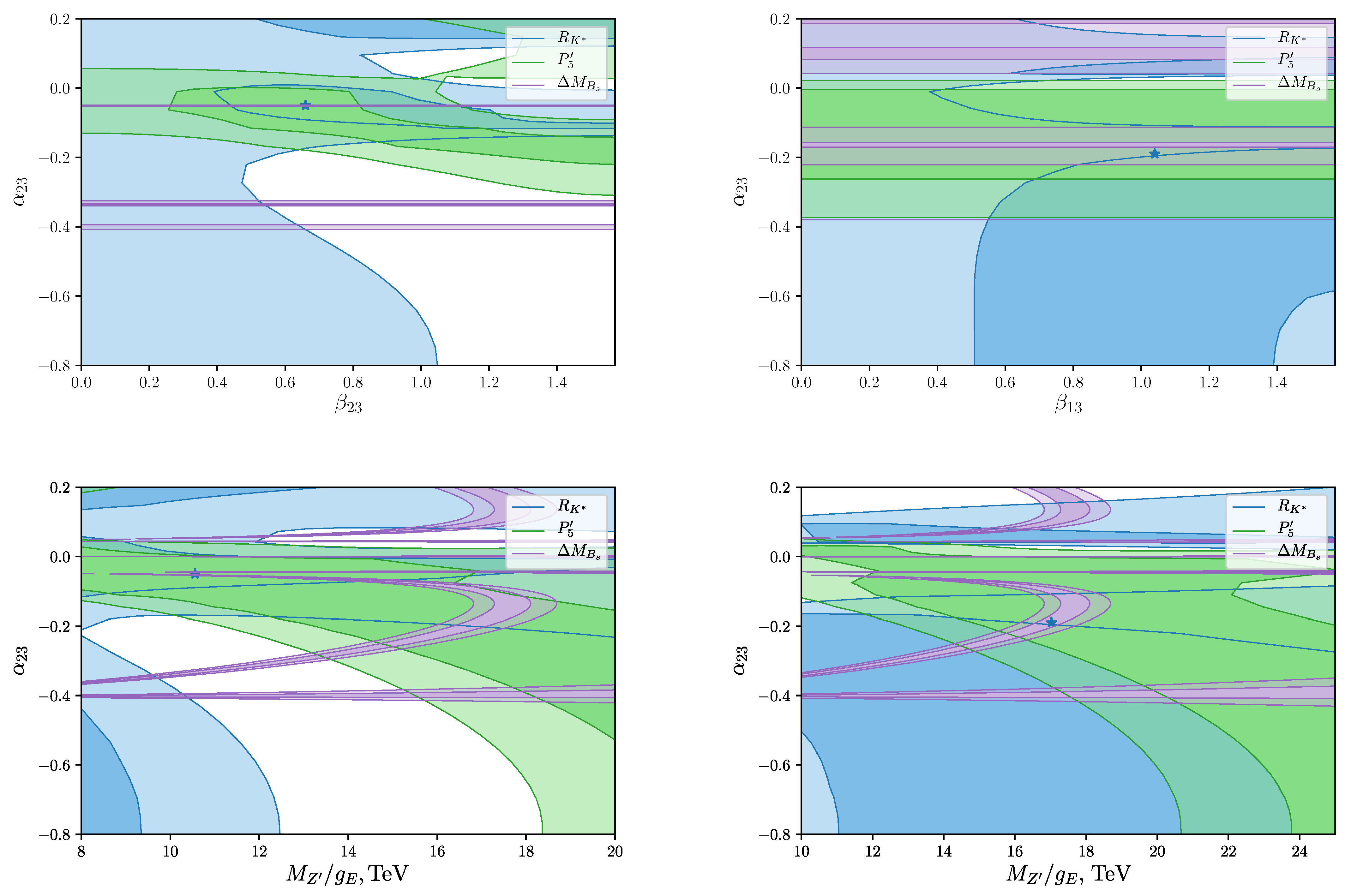
Taking into account all the above-mentioned experimental constraints, we find the allowed parameter space in the model. We consider the log-likelihood function incorporating the experimental measurements, and fit the three parameters , , and either or . We assume that , since negative angles give rise to the negative contribution to favoured by model-independent studies (see, e.g., [17]).
Figure 1 demonstrates how one- and three-sigma regions for different constraints overlap. The blue, green and purple regions depict bounds due to , , and , respectively. In spite of large uncertainty, the constraint on the mixing restricts and is not shown.
The best-fit points are obtained by means of Iminuit package [29] that utilizes the MINOS algorithm [30]. One can see that the quark mixing angle is tightly bounded near () and (). The minimum of the log-likelihood function correspond to our benchmark points (BMPs):
where we also indicate intervals obtained from the fit.
It is clear that it is the bound on coming from the mixing that severely restricts . The recent lattice results [31] imply that the SM contribution to is slightly larger than the experimental central value. In our model we have operators involving RH currents that can alleviate the difference. Indeed, adopting the formula from [13] to our case
we see that for it is possible to achieve .
Given the formulas for and (see Equations (14) and (17) of reference [32]), one can show that in the considered scenarios the differences ()
control the sign of the corrections to and . From Equation (38) we deduce that for either and () or , (). Clearly, the first scenario is disfavored by current experimental bounds. Nevertheless, we analyse both of them and examine whether the flavour anomalies can be accounted for, or at least, relaxed in comparison with the SM.
To get separate bounds on and we consider constraints on production at the LHC (see also, reference [33]). We take into account the results of LHC searches [27,34] and [35]. To estimate relevant cross-section we use the following simplified expression:
where is the spin of , and the final states are either or . The dimensionless factors
are given in terms of quark distributions and are evaluated at the scale . To estimate the cross-section we use the MSTW2008NLO [36] set of PDFs and the code ManeParse [37]. For the dilepton final state we take into account the leading QCD corrections by introducing a K-factor (see e.g., reference [38]). In our study we assume that all SUSY particles coupled to are much heavier that the boson, so can only decay via the interactions given in (28).
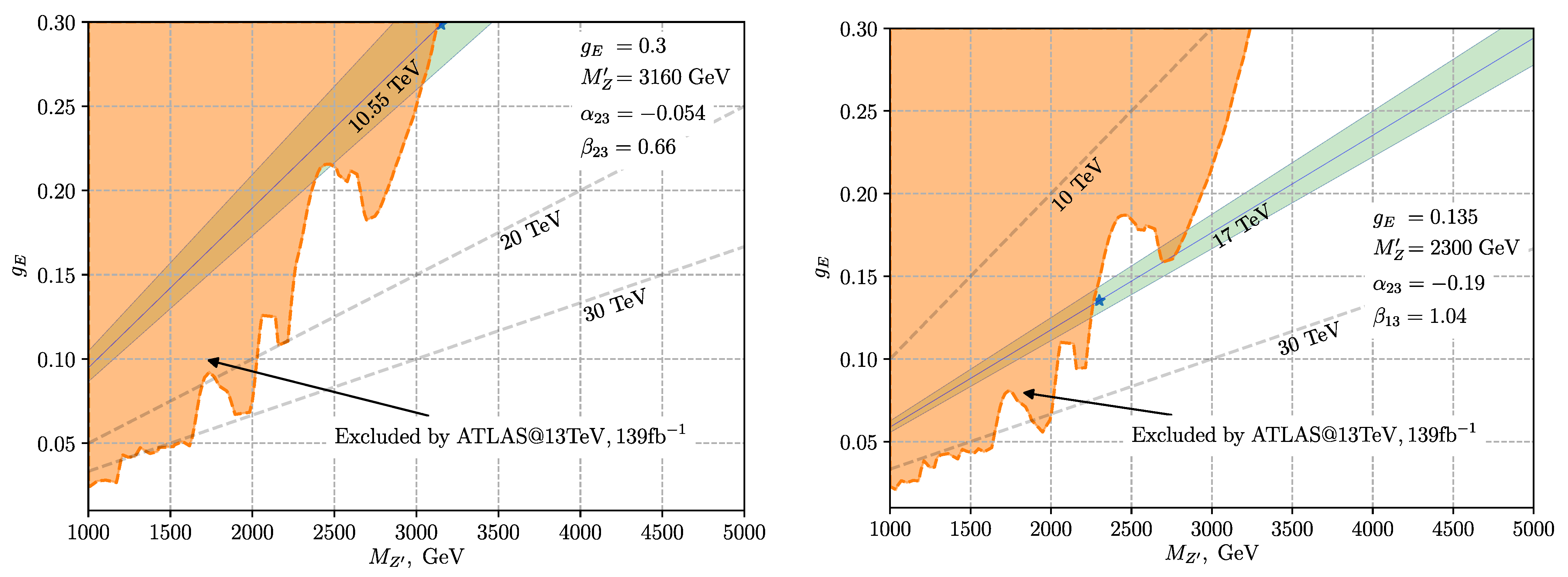
In Figure 2 we present the regions in the plane for fixed values of the angles corresponding to our BMPs, which are excluded by recent searches [27] . The constraints due to turn out to be much weaker. It is worth noting that larger values of the quark mixing angle give rise to a more restrictive bound on the parameter space. On the contrary, non-zero values of can reduce the coupling and, thus, relax the corresponding constraints.
Let us also mention that the value of the coupling at the weak scale can be bounded from above by the requirement that there should be no Landau pole up to GeV (Planck scale). Given the one-loop beta-function
one can deduce that (see also [24])
which motivates our choice of the upper limit in Figure 2.
One can see that BMP1 with 10.55 TeV lies just at the boundary of the excluded region, which make this point very unnatural. On the contrary, there is some freedom in the choice of and for BMP2 with 17 TeV, we assume that our BMP2 has minimal possible value of GeV with the corresponding .
Table 2 presents the model predictions for our benchmark points. The uncertainties given in Table 2 for the observables are related to the variation of parameters and are calculated using the Flavio (2.0.0) [16] package. For the LHC cross-sections at 13 and 14 TeV we give our estimates of the upper bounds since we neglect possible decays of to non-SM particles.
The estimated uncertainties for are rather big, which indicates that the scenarios are fine-tuned. Nevertheless, we see that both our benchmark points can easily account for , and in the central region. As we discussed earlier, we have different predictions for and in two considered cases. While the tension in can be alleviated, suggests that BMP1 is excluded. For BMP2 the model can accommodate smaller values of . Yet we predict , so future measurements of and can either favour or exclude the scenario.
In the Table 2 we also add our predictions for and . The BaBar Collaboration give the following 90% C.L. upper limits [19]:
The computed values are far below current experimental bounds (56). Unfortunately, the model does not produce sufficiently large to be observed at Belle II [39] (5 ).
5. Conclusions
We investigated the possibility to accommodate for the well-known flavour anomalies in the context of a supersymmetric extension of the SM with non-holomorphic soft terms. Contrary to previous studies, we extend the analysis to account not only for the quark and lepton masses together with the CKM matrix but also for the PMNS mixing of neutrinos. Moreover, we enumerated all relevant mixing parameters in quark and lepton sectors and, in addition to encoded in CKM and PMNS matrices, introduce four CP-conserving angles and four CP-violating phases.
To simplify our phenomenological analysis we restricted ourselves to the CP-conserving scenario with two additional angles: in the quark sector and either or in the lepton sector. We considered four-dimensional parameter space , computed relevant Wilson coefficients, and took into account experimental flavour data to fit the ratio of the mass and the coupling together with the additional fermion mixing angles.
Our analysis demonstrated that the most restrictive bound comes from the mixing. Nevertheless, due to the presence of right-handed operators, it is possible to relax the tension between the SM prediction and the experimental value. Another interesting observation is the hierarchy between and . In the considered scenarios we either have () or (). Unfortunately, the case give rise to and it is hard to accommodate the anomaly. We took into account the results of LHC searches and found viable points with GeV and . We also considered lepton-flavour violating semileptonic decays of B mesons predicted in the model. Unfortunately, the branching ratios and are far below current and future experimental limits.
Of course, our analysis is far from complete and we plan to extend it, e.g., by computing more observables and considering scenarios with CP-violation. We also expect that the case when both and are non-zero has richer phenomenology.
Finally, let us mention that the parametrization of the effective Yukawa matrices in terms of additional angles and phases proposed in the paper can be used in comprehensive analysis of the full model with the SARAH/SPheno toolkit [40].
Author Contributions
A.B. and A.M. contributed equally to the manuscript. Both authors have read and agreed to the published version of the manuscript.
Funding
This work was funded by Grant of the Russian Federation Government, Agreement No. 14.W03.31.0026 from 15.02.2018.
Acknowledgments
The authors are grateful to D. Straub for correspondence regarding the Flavio code.
Conflicts of Interest
The authors declare no conflict of interest.
References
- Aaij, R.; Adeva, B.; Adinolfi, M.; Adrover, C.; Affolder, A.; Ajaltouni, Z.; Albrecht, J.; Alessio, F.; Alexander, M.; Ali, S.; et al. Measurement of Form-Factor-Independent Observables in the Decay B0→K*0μ+μ−. Phys. Rev. Lett. 2013, 111, 191801. [Google Scholar] [CrossRef] [Green Version]
- Egede, U.; Hurth, T.; Matias, J.; Ramon, M.; Reece, W. New observables in the decay mode B¯d→K¯*0l+l−. JHEP 2008, 11, 032. [Google Scholar] [CrossRef] [Green Version]
- Abdesselam, A.; Adachi, I.; Adamczyk, K.; Aihara, H.; Al Said, S.; Arinstein, K.; Arita, Y.; Asner, D.M.; Aso, T.; Atmacan, H.; et al. Angular analysis of B0→K*(892)0ℓ+ℓ−. In Proceedings of the LHC Ski 2016: A First Discussion of 13 TeV Results, Obergurgl, Austria, 10–15 April 2016. [Google Scholar]
- Descotes-Genon, S.; Hurth, T.; Matias, J.; Virto, J. Optimizing the basis of B→K*ll observables in the full kinematic range. JHEP 2013, 5, 137. [Google Scholar] [CrossRef] [Green Version]
- Aaij, R.; Beteta, C.A.; Ackernley, T.; Adeva, B.; Adinolfi, M.; Afsharnia, H.; Aidala, C.A.; Aiola, S.; Ajaltouni, Z.; Akar, S.; et al. Measurement of CP-Averaged Observables in the B0→K*0μ+μ− Decay. Phys. Rev. Lett. 2020, 125, 011802. [Google Scholar] [CrossRef] [PubMed]
- Descotes-Genon, S.; Hofer, L.; Matias, J.; Virto, J. On the impact of power corrections in the prediction of B→K*μ+μ− observables. JHEP 2014, 12, 125. [Google Scholar] [CrossRef] [Green Version]
- Aaij, R.; Adeva, B.; Adinolfi, M.; Affolder, A.; Ajaltouni, Z.; Akar, S.; Albrecht, J.; Alessio, F.; Alexander, M.; Ali, S.; et al. Test of lepton universality using B+→K+ℓ+ℓ− decays. Phys. Rev. Lett. 2014, 113, 151601. [Google Scholar] [CrossRef] [Green Version]
- Aaij, R.; Adeva, B.; Adinolfi, M.; Ajaltouni, Z.; Akar, S.; Albrecht, J.; Alessio, F.; Alexander, M.; Ali, S.; Alkhazov, G.; et al. Test of lepton universality with B0→K*0ℓ+ℓ− decays. JHEP 2017, 8, 055. [Google Scholar] [CrossRef] [Green Version]
- Aaij, R.; Beteta, C.A.; Adeva, B.; Adinolfi, M.; Aidala, C.A.; Ajaltouni, Z.; Akar, S.; Albicocco, P.; Albrecht, J.; Alessio, F.; et al. Search for lepton-universality violation in B+→K+ℓ+ℓ− decays. Phys. Rev. Lett. 2019, 122, 191801. [Google Scholar] [CrossRef] [Green Version]
- Bifani, S.; Descotes-Genon, S.; Romero Vidal, A.; Schune, M.H. Review of Lepton Universality tests in B decays. J. Phys. G 2019, 46, 023001. [Google Scholar] [CrossRef] [Green Version]
- Abdesselam, A.; Adachi, I.; Adamczyk, K.; Ahn, J.K.; Aihara, H.; Said, S.A.; Arinstein, K.; Arita, Y.; Asner, D.M.; Atmacan, H.; et al. Test of lepton flavor universality in B→K*ℓ+ℓ− decays at Belle. arXiv 2019, arXiv:1904.02440. [Google Scholar]
- Artuso, M.; Borissov, G.; Lenz, A. CP violation in the system. Rev. Mod. Phys. 2016, 88, 045002. [Google Scholar] [CrossRef] [Green Version]
- Di Luzio, L.; Kirk, M.; Lenz, A.; Rauh, T. ΔMs theory precision confronts flavour anomalies. JHEP 2019, 12, 009. [Google Scholar] [CrossRef] [Green Version]
- Amhis, Y.S.; Banerjee, S.; Ben-Haim, E.; Bona, M.; Bozek, A.; Bozzi, C.; Brodzicka, J.; Chrzaszcz, M.J.; Dingfelder, J.C.; Egede, U.; et al. Averages of b-hadron, c-hadron, and τ-lepton properties as of 2018. arXiv 2019, arXiv:1909.12524. [Google Scholar]
- Zyla, P.; Barnett, R.M.; Beringer, J.; Dahl, O.; Dwyer, D.A.; Groom, D.E.; Lin, C.-J.; Lugovsky, K.S.; Pianori, E.; Robinson, D.J.; et al. Review of Particle Physics. PTEP 2020, 2020, 083C01. [Google Scholar] [CrossRef]
- Straub, D.M. flavio: A Python package for flavour and precision phenomenology in the Standard Model and beyond. arXiv 2018, arXiv:1810.08132. [Google Scholar]
- Altmannshofer, W.; Niehoff, C.; Stangl, P.; Straub, D.M. Status of the B→K*μ+μ− anomaly after Moriond 2017. Eur. Phys. J. C 2017, 77, 377. [Google Scholar] [CrossRef] [Green Version]
- Aubert, B.; Bona, M.; Boutigny, D.; Karyotakis, Y.; Lees, J.P.; Poireau, V.; Prudent, X.; Tisserand, V.; Zghiche, A.; Tico, J.G.; et al. Search for the decay B+→K+τ∓μ±. Phys. Rev. Lett. 2007, 99, 201801. [Google Scholar] [CrossRef] [Green Version]
- Lees, J.; Raven, H.G.; Collaboration BABAR. A search for the decay modes B+−→h+−τ+−l. Phys. Rev. D 2012, 86, 012004. [Google Scholar] [CrossRef] [Green Version]
- Aebischer, J.; Altmannshofer, W.; Guadagnoli, D.; Reboud, M.; Stangl, P.; Straub, D.M. B-decay discrepancies after Moriond 2019. Eur. Phys. J. C 2020, 80, 252. [Google Scholar] [CrossRef] [Green Version]
- Altmannshofer, W.; Gori, S.; Pospelov, M.; Yavin, I. Quark flavor transitions in Lμ−Lτ models. Phys. Rev. D 2014, 89, 095033. [Google Scholar] [CrossRef] [Green Version]
- Allanach, B.; Queiroz, F.S.; Strumia, A.; Sun, S. Z′ models for the LHCb and g−2 muon anomalies. Phys. Rev. D 2016, 93, 055045. [Google Scholar] [CrossRef]
- Demir, D.A.; Kane, G.L.; Wang, T.T. The Minimal U(1)’ extension of the MSSM. Phys. Rev. D 2005, 72, 015012. [Google Scholar] [CrossRef] [Green Version]
- Duan, G.H.; Fan, X.; Frank, M.; Han, C.; Yang, J.M. A minimal U(1)′ extension of MSSM in light of the B decay anomaly. Phys. Lett. 2019, B789, 54–58. [Google Scholar] [CrossRef]
- Allanach, B.; Gripaios, B.; Tooby-Smith, J. Anomaly cancellation with an extra gauge boson. Phys. Rev. Lett. 2020, 125, 161601. [Google Scholar] [CrossRef]
- Allanach, B. U(1)B3-L2 Explanation of the Neutral Current B-Anomalies. arXiv 2020, arXiv:2009.02197. [Google Scholar]
- Aad, G.; Abbott, B.; Abbott, D.C.; Abdinov, O.; Abud, A.A.; Abeling, K.; Abhayasinghe, D.K.; Abidi, S.H.; Abouzeid, O.; Abraham, N.; et al. Search for high-mass dilepton resonances using 139 fb-1 of pp collision data collected at =13 TeV with the ATLAS detector. Phys. Lett. 2019, B796, 68–87. [Google Scholar] [CrossRef]
- Borzumati, F.; Farrar, G.R.; Polonsky, N.; Thomas, S.D. Soft Yukawa couplings in supersymmetric theories. Nucl. Phys. B 1999, 555, 53–115. [Google Scholar] [CrossRef] [Green Version]
- Dembinski, H.; Ongmongkolkul, P.; Deil, C.; Hurtado, D.M.; Schreiner, H.; Feickert, M.; Andrew; Burr, C.; Rost, F.; Pearce, A. Scikit-Hep/Iminuit: v2.3.0. Available online: https://zenodo.org/record/4460551#.YA_XB1kzZhF (accessed on 11 January 2021).
- James, F.; Roos, M. Minuit—A System for Function Minimization and Analysis of the Parameter Errors and Correlations. Comput. Phys. Commun. 1975, 10, 343–367. [Google Scholar] [CrossRef]
- Aoki, S.; Aoki, Y.; Bečirević, D.; Blum, T.; Colangelo, G.; Collins, S.; Morte, M.D.; Dimopoulos, P.; Dürr, S.; Fukaya, H.; et al. FLAG Review 2019: Flavour Lattice Averaging Group (FLAG). Eur. Phys. J. C 2020, 80, 113. [Google Scholar] [CrossRef] [Green Version]
- D’Amico, G.; Nardecchia, M.; Panci, P.; Sannino, F.; Strumia, A.; Torre, R.; Urbano, A. Flavour anomalies after the RK* measurement. JHEP 2017, 9, 010. [Google Scholar] [CrossRef]
- Allanach, B.; Butterworth, J.; Corbett, T. Collider constraints on Z′ models for neutral current B-anomalies. JHEP 2019, 8, 106. [Google Scholar] [CrossRef] [Green Version]
- Sirunyan, A.M.; Tumasyan, A.; Adam, W.; Ambrogi, F.; Asilar, E.; Bergauer, T.; Brandstetter, J.; Brondolin, E.; Dragicevic, M.; Erö, J.; et al. Search for high-mass resonances in dilepton final states in proton-proton collisions at = 13 TeV. JHEP 2018, 6, 120. [Google Scholar] [CrossRef] [Green Version]
- Aad, G.; Abbott, B.; Abbott, D.C.; Abud, A.A.; Abeling, K.; Abhayasinghe, D.K.; SHAbouZeid, O.S.A.; Abraham, N.L.; Abramowicz, H.; Abreu, H.; et al. Search for resonances in fully hadronic final states in pp collisions at = 13 TeV with the ATLAS detector. JHEP 2020, 10, 061. [Google Scholar] [CrossRef]
- Martin, A.D.; Stirling, W.J.; Thorne, R.S.; Watt, G. Parton distributions for the LHC. Eur. Phys. J. 2009, C63, 189–285. [Google Scholar] [CrossRef] [Green Version]
- Clark, D.B.; Godat, E.; Olness, F.I. ManeParse: A Mathematica reader for Parton Distribution Functions. Comput. Phys. Commun. 2017, 216, 126–137. [Google Scholar] [CrossRef] [Green Version]
- Fuks, B.; Klasen, M.; Ledroit, F.; Li, Q.; Morel, J. Precision predictions for Z′-production at the CERN LHC: QCD matrix elements, parton showers, and joint resummation. Nucl. Phys. 2008, B797, 322–339. [Google Scholar] [CrossRef] [Green Version]
- Bhattacharya, B.; Datta, A.; Guévin, J.P.; London, D.; Watanabe, R. Simultaneous Explanation of the RK and RD(*) Puzzles: A Model Analysis. JHEP 2017, 1, 015. [Google Scholar] [CrossRef]
- Staub, F.; Ohl, T.; Porod, W.; Speckner, C. A Tool Box for Implementing Supersymmetric Models. Comput. Phys. Commun. 2012, 183, 2165–2206. [Google Scholar] [CrossRef] [Green Version]
Figure 1.
Overlapping 1-3 regions due to experimental constraints on the indicated observables for (left) and (right). Our benchmark points (BMPs) are marked with an asterisk.
Figure 1.
Overlapping 1-3 regions due to experimental constraints on the indicated observables for (left) and (right). Our benchmark points (BMPs) are marked with an asterisk.

Figure 2.
Constraints on and due to the searches [27]. The left figure corresponds to , while the right one to . The benchmark points are indicated and the corresponding parameters are shown. The shaded region is excluded. Straight lines correspond to different values of in TeV, and the green band reflects the uncertainty of the fitted value.


Table 1.
The anomaly-free charges considered in the paper.
| Field | Field | Field | |||
|---|---|---|---|---|---|
| 0 | 0 | 0 | |||
| 0 | 0 | ||||
| 0 | S |
Table 2.
Model predictions for the best fit values. BMP1 corresponds to , , GeV, , while BMP2 to , , GeV, . We do not give experimental bounds [27] on in the table since they are different for different masses.
Publisher’s Note: MDPI stays neutral with regard to jurisdictional claims in published maps and institutional affiliations. |
© 2021 by the authors. Licensee MDPI, Basel, Switzerland. This article is an open access article distributed under the terms and conditions of the Creative Commons Attribution (CC BY) license (http://creativecommons.org/licenses/by/4.0/).
Share and Cite
MDPI and ACS Style
Bednyakov, A.; Mukhaeva, A. Flavour Anomalies in a U(1) SUSY Extension of the SM. Symmetry 2021, 13, 191. https://doi.org/10.3390/sym13020191
AMA Style
Bednyakov A, Mukhaeva A. Flavour Anomalies in a U(1) SUSY Extension of the SM. Symmetry. 2021; 13(2):191. https://doi.org/10.3390/sym13020191
Chicago/Turabian StyleBednyakov, Alexander, and Alfiia Mukhaeva. 2021. "Flavour Anomalies in a U(1) SUSY Extension of the SM" Symmetry 13, no. 2: 191. https://doi.org/10.3390/sym13020191
Note that from the first issue of 2016, this journal uses article numbers instead of page numbers. See further details here.