Solving the Asymmetry Multi-Objective Optimization Problem in PPPs under LPVR Mechanism by Bi-Level Programing

Abstract

Optimizing the cost and benefit allocation among multiple players in a public-private partnership (PPP) project is recognized to be a multi-objective optimization problem (MOP). When the least present value of revenue (LPVR) mechanism is adopted in the competitive procurement of PPPs, the MOP presents asymmetry in objective levels, control variables and action orders. This paper characterizes this asymmetrical MOP in Stackelberg theory and builds a bi-level programing model to solve it in order to support the decision-making activities of both the public and private sectors in negotiation. An intuitive algorithm based on the non-dominated sorting genetic algorithm III (NSGA III) framework is designed to generate Pareto solutions that allow decision-makers to choose optimal strategies from their own criteria. The effectiveness of the model and algorithm is validated via a real case of a highway PPP project. The results reveal that the PPP project will be financially infeasible without the transfer of certain amounts of exterior benefits into supplementary income for the private sector. Besides, the strategy of transferring minimum exterior benefits is more beneficial to the public sector than to users.

1. Introduction

Public-private partnerships (PPP) have been applied worldwide as a financing instrument to provide public infrastructures and services. In a PPP project, the private sector is usually responsible for the operation of the project and for providing part of the initial investments, with a return on governmental subsidies, user payments or extraneous earnings derived from exterior benefits generated by the project [1]. In other words, when the private sector benefits increase, the costs from the public side are increased.

In the past few decades, the view that cost or benefit allocation among multiple players in a PPP project is actually a multi-objective optimization problem (MOP) has been formed. Koppenjan (2005) investigated the reasons for the stagnation of transport PPP in the Netherlands, finding that the mutually exclusive goals of the public and private sectors affected the sustainability of cooperation [2]. Papajohn (2011) put forward the view that the public is an important stakeholder of PPPs whose interest would be damaged if the government uses PPP to make excessive investments [3]. Garvin (2010) believed that PPP decision-making from the government needs to justify its economic feasibility by realizing “value for money” [4]. Xu (2014) et al. found that the government attaches too much attention to the way of measuring subsidies rather than the number of subsidies actually paid, leading to unnecessary guarantees for the private sector [5]. For a toll road with exogenous demand risk, Kayhan and Jenkins (2016) proposed that the government needs to justify the minimum traffic guarantee (MIG) policy granted to the private sector [6].

Besides these qualitative analyses, Rouhani (2015) established pricing optimization models for the planning of a transport PPP project with the theories of user equilibrium (UE) and system optimization (SO) and suggested that a mixed public and private tolling scheme should be adopted to realize Pareto improvement for all stakeholders [7]. Song et al. (2018) built a MOP model to coordinate the interests of the government and a private firm and found that MIG is not always the best strategy for the government to provide revenue guarantees [8]. In addition to user charges and subsidies, the factors involved in a PPP investment and return strategy include initial investment sharing [9], concession terms [10,11,12] and other forms of revenue guarantee, such as the exterior benefits collected and transferred into supplementary incomes of the project [13,14].

Existing studies have discussed MOPs with symmetry optimization objectives in PPPs, in which all players have the motivation to maximize their own benefits (or minimize costs). However, the fact that the benefit maximization of the private sector does not mean profit maximization in all circumstances produces asymmetrical optimization objectives in the case of the MOP defined above. A typical scenario in practice is the use of the least present value of revenue (LPVR) mechanism in the competitive procurement of a PPP project. Under the LPVR mechanism, the concession contract will be awarded to companies in the private sector who bid with the least present value of revenue discounted at a predetermined return rate [15]. In that case, the private sector pursues an acceptable sub-optimal strategy, but not the maximum present value of revenue, in order to win the contract [16].

Besides, this asymmetry is reflected in the differences of control variables and action orders. Commonly, the private sector decides the user charges and concession terms within an approved range based on market experience, and the initial investment sharing, operation subsidies and transferred exterior benefits are decided by the public sector, since they are related to the current and future fiscal status. The public sector usually initializes the negotiation by proposing a primary strategy to solicit the potential private sector companies, who will respond with a bidding strategy following the decision-maker.

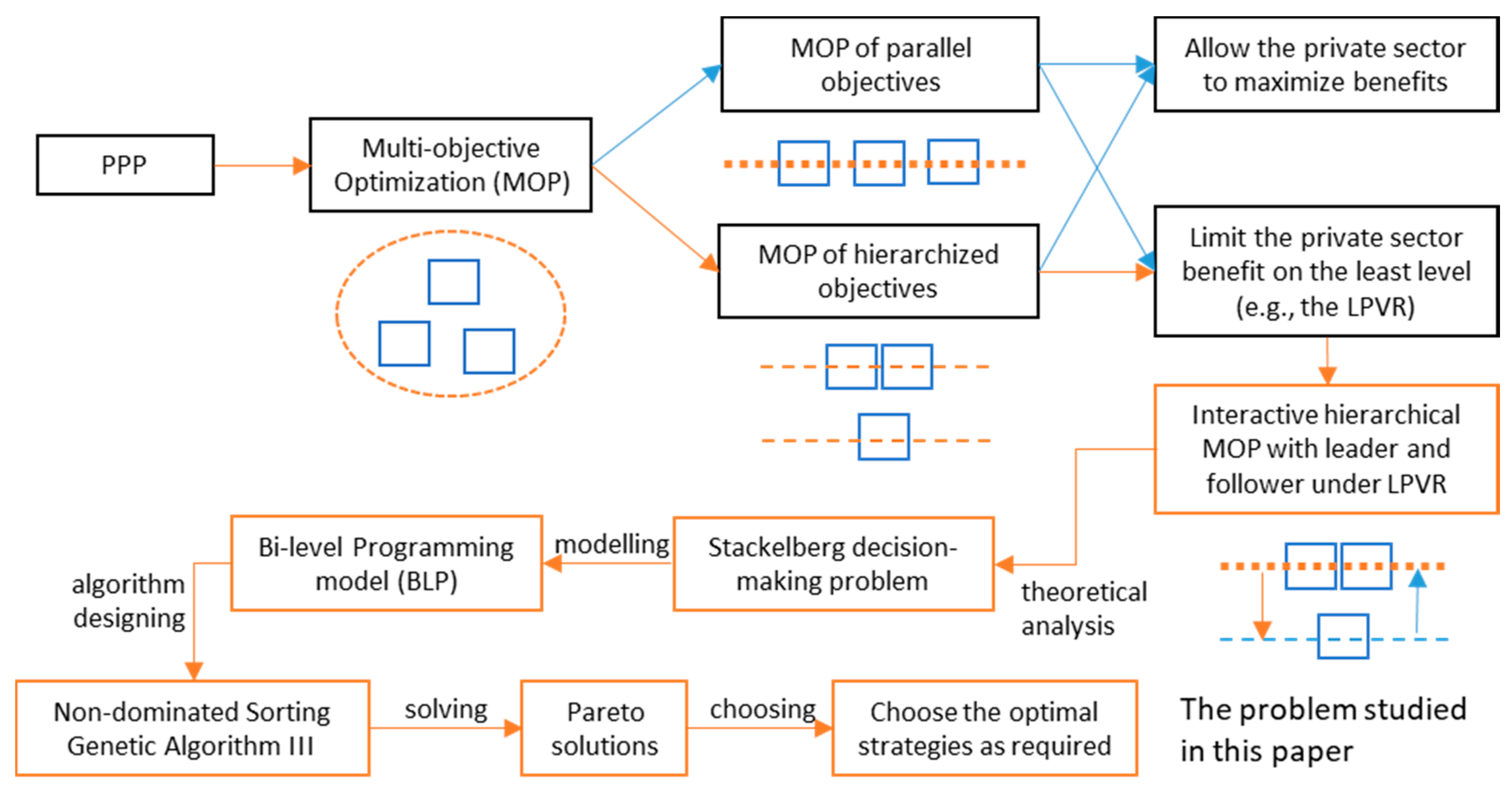
This paper studies the asymmetrical MOP in PPPs under the LPVR mechanism to provide references for bidding strategies for decision-makers from both the public and private sectors. Stackelberg game theory is used to characterize the decision-making process. A bi-level programing (BLP) model is built, taking the public sector as the decision-maker at the upper level and the private sector as the decision-maker at the lower level. The main idea of this paper is displayed in Figure 1.

The rest of this paper is organized as follows. In Section 2, the analysis of the asymmetrical decision-making MOP based on the theories of Stackelberg game theory and the LPVR mechanism is presented; in Section 3, a BLP model is constructed, and the manner in which objectives in the BLP model are optimized is illustrated; in Section 4, a non-dominated sorting genetic algorithm (NSGA)-based method is designed to solve the BLP model; in Section 5, a highway PPP case is given to validate the effectiveness of the model and algorithm, and policy suggestions are made upon the discussion of results; finally, in Section 6, conclusions are presented.

2. Theoretical Analysis of the MOP under LPVR

2.1. The LPVR Mechanism

The original idea of LPVR is a flexible-term concession; in other words, the concession term is tied to certain return on investment (ROI) indicators for the private sector [17]. When future demand is better than expected, the private sector is allowed to end the contract earlier than estimated. In contrast, when the future demand is not as optimistic as expected, the private sector is allowed to extend the concession term in order to achieve the pre-set ROI. According to Engle et al. (1997, 2001), the pre-set ROI will be used at a discounted rate to calculate the private sector’s present value of revenue (PVR), which has been taken as the key variable in the tender of the concession contract [15,18]. The private sector with the least PVR, i.e., the LPVR, will be granted the concession contract. Equation (1) presents the general expression of the LPVR [18]:

$$\mathrm{LPVR}=\min \left(-I_0+{\displaystyle \sum _{i=1}^{\tau }\frac{\rho q_i-m_i}{{(1+r^{\mathrm{pri}})}^i}}\right)$$

(1)

where ${\mathrm{LPVR}}^{\mathrm{pri}}$ is the net present value calculated in the base year; $C_0$ is the initial investment that is paid by the private sector in a PPP project; $\tau$ is the estimated concession term; $\rho$ is the unit charge from users; $q_i$ is the estimated quantity of service or products provided by the project in the i-th year; and $m_i$ is the maintaining and operating cost in i-th year. Theoretically, an LPVR of 0 means that the private sector obtains revenues that are exactly equal to the costs incurred.

In the context of a PPP project, the net present value of revenue of the private sector—the PVR of the private sector—is also affected by decisions from the public sector, which cause variations in both the initial investment section and operation section. Such variations are shown in Equation (2), where ${\Delta }^{(1)}$ is the initial investment shared by the public sector and ${\Delta }_i^{(2)}$ contains the operation subsidy and consumed exterior benefits of the i-th year. During the negotiation, the private sector needs to find the least PVR (the LPVR) to win in the bidding process.

$${\mathrm{PVR}}^{\mathrm{pri}}=-(I_0-{\Delta }^{(1)})+{\displaystyle \sum _{i=1}^{\tau }\frac{\rho q_i-m_i+{\Delta }_i^{(2)}}{{(1+r^{\mathrm{pri}})}^i}}$$

(2)

2.2. The Interactive Stackelberg Decision-Making Process

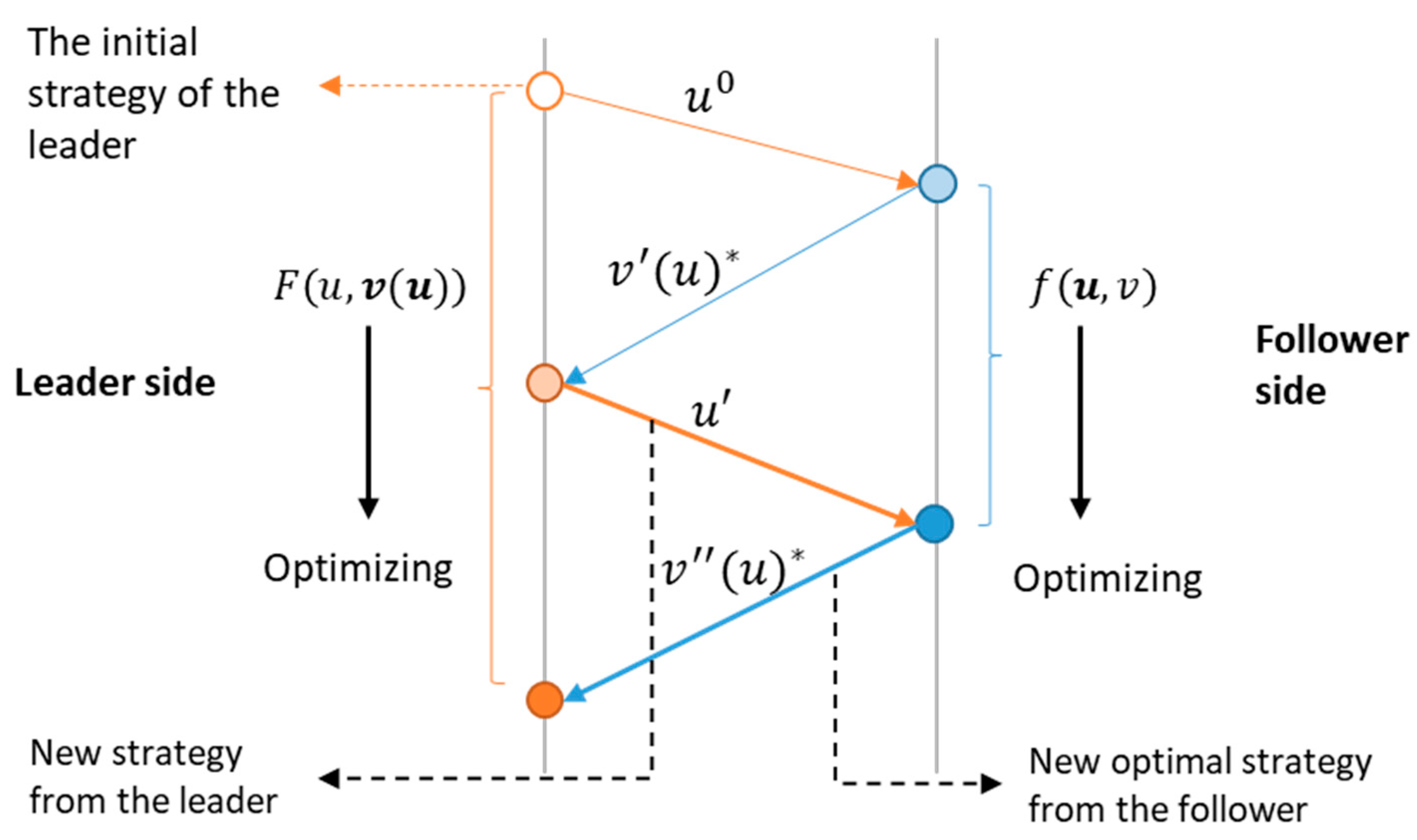
Equation (2) shows that the private sector benefits are affected by the public sector’s decisions. Correspondingly, the public sector benefits are also affected by the decisions of the private sector when the control variables $\rho$ and $\tau$ of the private sector are used as input parameters for calculating benefits (or costs) at the public side. Supposing ${\Delta }^{(1)}$ and ${\Delta }_i^{(2)}$ in Equation (2) are determined by strategy $u$ proposed by the public sector, and $\rho$ and $\tau$ are the elements of strategy $v$ proposed by the private sector, an interactive decision-making process with the public sector as the leader and the private sector as the follower is shown in Figure 2.

The above interactive decision-making process could be characterized by the Stackelberg decision-making problem [19], which has the following characteristics in general: (1) each decision-maker has specific objectives and control variables, and their strategy will affect the benefits of the others as well as their own; (2) the objectives of different decision-makers are located in different levels, presenting a hierarchical decision-making structure—the upper decision-maker has higher priority in terms of the action order than the lower decision-maker; (3) the decisions of the upper and lower level impact each other, thus forming a relationship of mutual influence and restriction; and (4) the final decision will be a globally feasible solution that satisfies all decision-makers as much as possible.

The Stackelberg decision-making problem could be solved by a bi-level programing (BLP) model [20]. The general form of the BLP model consists of an upper programing (UP) problem and lower programing (LP) problem, which could be expressed as Equations (3)–(6), as shown in [21].

(UP)

$$\underset{u}{\min }F\left(u,v(u)\right)$$

(3)

subject to

$$G\left(u,v(u)\right)\le 0$$

(4)

(LP)

$$\underset{v}{\min }f(u,v)$$

(5)

subject to

$$g(u,v)\le 0$$

(6)

where $F\left(u,v(u)\right)$, $u$ and $G\left(u,v(u)\right)$ are the objective function, vector of control variables and constraint of the upper level decision-maker, respectively; $f(u,v)$, $v$ and $g(u,v)$ are those of the lower decision-maker; and $u$ is used as the input parameter when calculating $f(u,v)$ and $v(u)$ is used as the input parameter when calculating $F\left(u,v(u)\right)$.

3. Modeling the Problem by Bi-Level Programing (BLP)

There are two prerequisites for both parties to participate in the PPP project: one is that the public sector should accomplish “value for money” (VFM)—the lifecycle costs paid in the PPP mode should be no more than that in the traditional investment mode (without private funding)—while the other one is that the private sector can obtain an actual return level that is no less than the pre-set rate of return. In other words, the values of VFM and LPVR are required to be positive to satisfy the two prerequisites.

Definitions of parameters and variables in the formulas of the model are listed in

Table A1. Notations and definitions of parameters and variables used in Section 3.1 and Section 3.2.

Notation	Definition
Input Parameters
$I$	Total investment of the project
$I{}^{\prime }$	Extra direct investment that can be used to deduct loans, usually arising from a specific finance source such as a public transfer payment from the central government
$n$	Construction term of the project
$q_i$	Traffic volume of the i-th year in operation period
$c_i$	Operation cost of the i-th year in operation period
$m_i$	Montage paid of the i-th year in operation period
$r_{\mathrm{nt}}$	The ratio of non-toll income making up to the toll income
$o_i$	Ancillary services revenue; i.e., the non-toll incomes of the i-th year in concession term, such as refueling, parking and catering
$r^{\mathrm{cap}}$	The proportion of equity capital funds
$r_j^{\mathrm{con}}$	The proportion of the funds invested in the j-th year of construction in the total investment
$r^{\mathrm{deb}}$	Rate of the debt fund
$r^{\mathrm{gov}}$	Discount rate of the public sector
$r^{\mathrm{pri}}$	Discount rate of the private sector
$e_i$	The exterior benefits generated from project implementation in the i-th year
Decision Variables
$\alpha$	Initial investment for construction shared by the public sector. The private sector’s share is notated as $1-\alpha$.
$\delta$	Subsidy per vehicle-kilometer
$\epsilon$	Ratio of exterior benefits to be collected
$\rho$	Toll of per vehicle-kilometer
$\tau$	Concession term

of Appendix A.

3.1. The Upper Programing (UP) Problem

The UP problem is a three-objective MOP that is used to minimize the lifecycle cost of the public sector, the payment level of users and the consumption of exterior benefits. The constraint for the public sector to participate in a PPP project is to realize “value for money”, i.e., the value of VFM should be non-negative. The objectives and constraints of the UP problem are formally expressed as follows:

$$\underset{\alpha ,\delta }{\min }G\left(\alpha ,\delta ,{\nu }_{(\alpha ,\delta ,\epsilon )}(\rho ,\tau )\right)$$

(7)

$$\underset{\rho }{\min }\rho$$

(8)

$$\underset{\epsilon }{\min }\epsilon$$

(9)

subject to

$$-\mathrm{VFM}\le 0$$

(10)

where $G\left(\alpha ,\delta ,{\nu }_{(\alpha ,\delta ,\epsilon )}(\rho ,\tau )\right)$ is the net present value of the lifecycle cost paid by the public sector under the PPP mode; $\rho$ is the unit toll per vehicle-kilometer, representing the payment level of users; and $\epsilon$ is the ratio of collected exterior benefits used as supplementary income for the project. ${\nu }_{(\alpha ,\delta ,\epsilon )}(\rho ,\tau )$ is the input variable combination of $\{{\rho }^{*},{\tau }^{*}\}$, which is solved by the lower programing (LP) model upon the upper decision $\{\alpha ,\delta ,\epsilon \}$. The full expression of the UP objective is:

$$G\left(\alpha ,\delta ,{\nu }_{(\alpha ,\delta ,\epsilon )}(\rho ,\tau )\right)={\displaystyle \sum _{j=1}^n\frac{\alpha I{r}^{\mathrm{cap}}{r}_j^{\mathrm{con}}}{{(1+r^{\mathrm{gov}})}^j}}+{\displaystyle \sum _{i=1+n}^{\tau +n}\frac{\delta q_i}{{(1+r^{\mathrm{gov}})}^i}}$$

(11)

which consists of two terms. The first term of Equation (11) is the net present value (NPV) of equity funds shared by the public sector, and the second term is the NPV of subsidies that the public sector expends during the whole operation period.

The value of VFM is defined as the difference between the lifecycle cost under traditional investment mode, called the public sector comparator (PSC) value, and that under the PPP mode expressed by $G\left(\alpha ,\delta ,{\nu }_{(\alpha ,\delta ,\epsilon )}(\rho ,\tau )\right)$. Under the traditional investment mode, the equity funds of construction investment and operation costs are all afforded by the public sector. The value of PSC can be expressed as:

$$\mathrm{PSC}={\displaystyle \sum _{j=1}^n\frac{I{r}^{\mathrm{cap}}{r}_j^{\mathrm{con}}}{{(1+r^{\mathrm{gov}})}^j}}-{\displaystyle \sum _{i=1+n}^{\tau +n}\frac{\rho q_i+o_i-c_i-m_i}{{(1+r^{\mathrm{gov}})}^i}}$$

(12)

and the value of VFM is

$$\begin{array}{cc}\hfill \mathrm{VFM}& =\mathrm{PSC}-G\left(\alpha ,\delta ,{\nu }_{(\alpha ,\delta ,\epsilon )}(\rho ,\tau )\right)\hfill \\ & ={\displaystyle \sum _{j=1}^n\frac{(1-\alpha )I{r}^{\mathrm{cap}}{r}_j^{\mathrm{con}}}{{(1+r^{\mathrm{gov}})}^j}}-{\displaystyle \sum _{i=1+n}^{\tau +n}\frac{(\rho -\delta )q_i+o_i-c_i-m_i}{{(1+r^{\mathrm{gov}})}^i}}\hfill \end{array}$$

(13)

3.2. The Lower Programing (LP) Problem

In the LP problem, the private sector company reduces their benefits due not to an original intention but to improve the chance of being selected as the partner, especially in a competitive bidding scenario under the LPVR mechanism. The objective function of the private sector company is to minimize their PVR, which is constrained by their own non-negative requirement. The model of the LP problem is formally expressed as follows:

$$\underset{\rho ,\tau }{\min }P(\alpha {}^{\prime },\delta {}^{\prime },\epsilon {}^{\prime },\rho ,\tau )$$

(14)

subject to

$$-P(\alpha {}^{\prime },\delta {}^{\prime },\epsilon {}^{\prime },\rho ,\tau )\le 0$$

(15)

where $P(\alpha {}^{\prime },\delta {}^{\prime },\epsilon {}^{\prime },\rho ,\tau )$ is the net present value of the private sector benefit, and $\{\alpha {}^{\prime },\delta {}^{\prime },\epsilon {}^{\prime }\}$ is given by the upper decision-maker (the public sector). The full expression of $P(\alpha {}^{\prime },\delta {}^{\prime },\epsilon {}^{\prime },\rho ,\tau )$ is:

$$P(\alpha {}^{\prime },\delta {}^{\prime },\epsilon {}^{\prime },\rho ,\tau )=-{\displaystyle \sum _{j=1}^n\frac{(1-\alpha )I{r}^{\mathrm{cap}}{r}_j^{\mathrm{con}}}{{(1+r^{\mathrm{pri}})}^j}}+{\displaystyle \sum _{i=1+n}^{\tau +n}\frac{(\rho +\delta )q_i+o_i-c_i-m_i+\epsilon e_i}{{(1+r^{\mathrm{pri}})}^i}}$$

(16)

3.3. Optimization of Objectives in the BLP Model

As is known, it is difficult to find an absolute optimal solution in a MOP with conflicted objectives in which a series of comparatively optimal solutions, called Pareto solutions, could be obtained. Each Pareto solution performs better for at least one objective and worse for at least one objective than other Pareto solutions [22]. Pareto solutions can leave the decision-makers with adequate space for strategies without any requirements of weighting the multiple objectives as one general objective in advance.

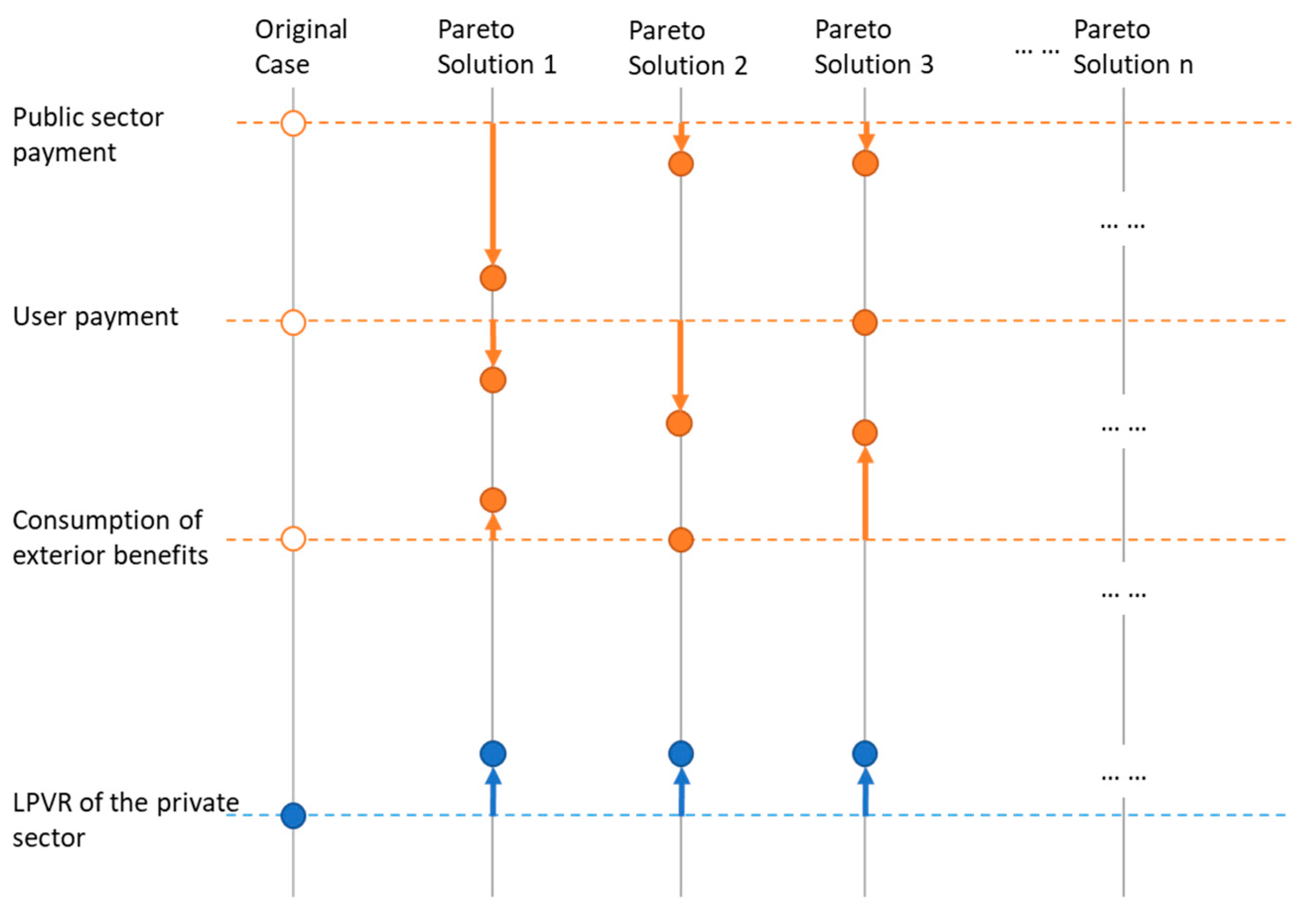
In this paper, Pareto solutions will be solved and then compared to the original case in a case study to determine which objectives are present and the degree to which they are optimized. Figure 3 shows the schematic of how the Pareto solutions are demonstrated in the final results. For instance, in Figure 3, Pareto solution 1 reduces the payment of the public sector and users but increases the consumption of exterior benefits (EB) and the LPVR of the private sector; Pareto solution 2 reduces the payment of the public sector and users, keeps the consumption of EB the same, and lifts the LPVR; and Pareto solution 3 reduces the public sector costs, keeps the user payment level the same, and increases the consumption of EB and LPVR. It is noticeable that when the value of LPVR is more than zero, this means that the private sector could obtain more revenue than expected.

4. NSGAIII Framework-Based Algorithm for the BLP Model

BLP models are difficult to solve directly because of their status as NP-hard problems. The model built in Section 3 adds even difficulty since the UP problem is a three-objective nonlinear MOP and the LP problem is a mixed-integer nonlinear problem. Interactions between the two levels are hardly predicted; thus, the widely used Karush-Kuhn-Tucker (KKT) conditions [23] or sensitivity analysis-based methods [24] would not work for this problem.

In studies [25,26,27,28] aimed at solving such complex BLP models in recent years, embedded-computational approaches are applied. In general, the outer layer of their framework contains a heuristic algorithm to solve the UP problem, such as the genetic algorithm (GA), simulated annealing (SA) and particle swarm optimization (PSO). Then, a specific algorithm is applied to provide the optimal solutions to the LP problem, which are used as input parameters to compute the UP problem.

In this paper, the general idea used to solve the complete BLP model is to create an embedded-computational framework. The algorithm of non-dominating GAs—known as NSGAIII—is used to solve the three-dimensional MOP in the upper level. Additionally, the algorithm based on variable discretization is taken to quickly produce optimal solutions to the LP problem. NSGAIII is an algorithm developed on the GA framework to solve many-objective problems (MaOPs) [29] and has a good reputation for improving the evenness and diversity of solutions via the elite selection strategy of “reference points” [30].

In the built BLP model, problems of both levels have independent constraints. Every individual in the final Pareto solution set of $\left\{\alpha ,\delta ,\epsilon ,\rho ,\tau \right\}$ should be globally feasible, i.e., satisfying the constraints of both the UP problem and the LP problem. In each part of the combination of $\left\{\alpha ,\delta ,\epsilon ,\rho ,\tau \right\}$, $\{\rho ,\tau \}$ is solved based on $\left\{\alpha ,\delta ,\epsilon \right\}$, and $\left\{\alpha ,\delta ,\epsilon \right\}$ is an optimal solution of the upper problem. There are two main targets of the algorithm design of the BLP model: (1) to ensure that the LP problem produces feasible solutions upon each decision from the UP; and (2) to create a fast searching technique, which is required to solve the LP problem to avoid embedded iterations that would consume too much computing time, since the algorithm of the UP problem is evolution-based.

4.1. Interception Strategy for Reparing Solutions of the UP Problem

The main idea of this strategy is to intercept the UP solution $\left\{\alpha ,\delta ,\epsilon \right\}$ that causes the LP not to be able to find a feasible solution under its own constraints. The interception strategy process includes the following steps.

Step 1: Generate N individuals of $\left\{\alpha ,\delta ,\epsilon ,{\rho }^{\max },{\tau }^{\max }\right\}$ by the GA operator. ${\rho }^{\max }$ and ${\tau }^{\max }$ are the upper limits of $\rho$ and $\tau$, respectively. N is the size of the population.

Step 2: Compute the value of the LP constraint function with N individuals of $\left\{\alpha ,\delta ,\epsilon ,{\rho }^{\max },{\tau }^{\max }\right\}$. Count the number of individuals which violate the LP constraint, and notate it as $n$.

Step 3: Repeat Step 1 and Step 2 for $n$ individuals of $\left\{\alpha ,\delta ,\epsilon ,{\rho }^{\max },{\tau }^{\max }\right\}$ until $n=0$.

4.2. Subsection Approximation Strategy for Optimizing the LP

When solving the LP, $\left\{\alpha ,\delta ,\epsilon \right\}$ is taken as the given parameter set. Besides this, $\tau$ is a set with a limited number of integer elements indicating the year of concession term, as $\tau =\{1,2,\cdots ,{\tau }^{\max }\}$. Thus, Equation (16) can be equivalently transformed into Equation(17):

$$F_{\mathrm{LP}}={\displaystyle \sum _{i=1}^{\tau }\rho {(1+r^{\mathrm{pri}})}^{-i}}$$

(17)

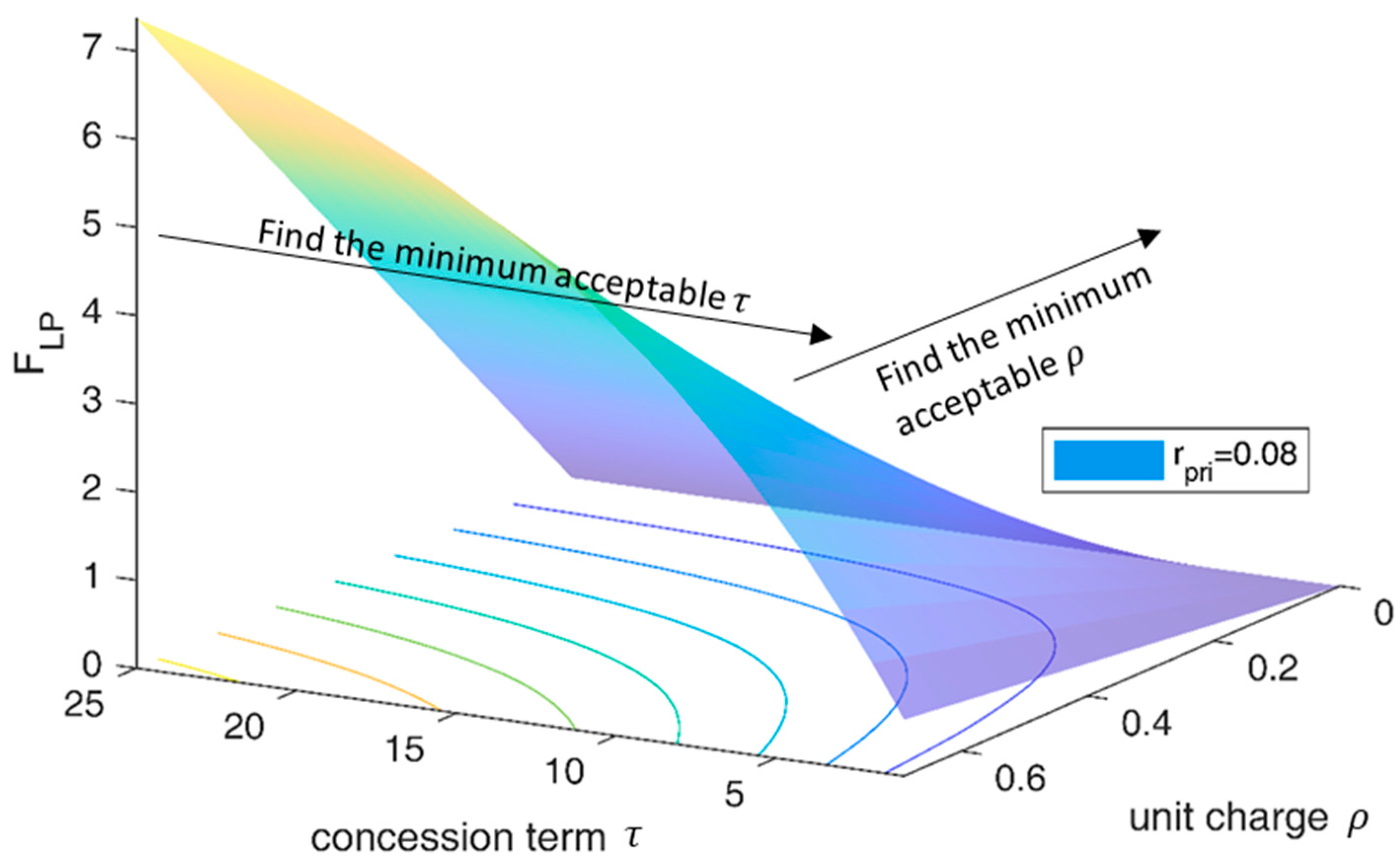
Figure 4 shows the three-dimensional surface diagram with contours of the functional relationships between $F_{\mathrm{LP}}$, $\rho$ and $\tau$, where $\rho$ is taken as a discretized variable. The $F_{\mathrm{LP}}$ value remains the same at different positions on the same contour line. It can be seen from Figure 2 that larger values of $\rho$ and $\tau$ produce larger values of $F_{\mathrm{LP}}$. Besides this, under the same value of $F_{\mathrm{LP}}$, $\rho$ and $\tau$ present a kind of inverse correlation. Assuming that the private sector is more averse to long-term concessions than charging lower prices, the process of the subsection approximation strategy includes the following steps.

Step 1: Discretize the continuous decision variable $\rho \in [{\rho }^{\min },{\rho }^{\max }]$ according to some acceptable precision. For example, ${\rho }^{\min }=0$ and ${\rho }^{\max }=0.69$ at a precision of 0.01; then, $\rho$ can be segmented into 70 pieces as $\rho =\{0.00,0.01,0.02,\cdots ,0.69\}$.

Step 2: According to the order that $\tau ={\tau }^{(1)},\tau ={\tau }^{(2)},\cdots ,\tau ={\tau }^{\max }$, for each $\left\{\alpha ,\delta ,\epsilon \right\}$ from the UP problem, calculate Equation (16) (the objective function of the LP), with the combination of $\{\alpha ,\delta ,\epsilon ,{\rho }^{\max },\tau \}$. Search for the first $\tau$ that makes $F_{\mathrm{LP}}\ge 0$, and then stop. Set that $\tau$ as $\tau {}^{\prime }$.

Step 3: According to the order that $\rho ={\rho }^{\left(1\right)},\rho ={\rho }^{\left(2\right)},\cdots ,\rho ={\rho }^{\max }$, for each $\{\alpha ,\delta ,\epsilon ,\rho ,\tau {}^{\prime }\}$, calculate Equation (16) with the combination of $\{\alpha ,\delta ,\epsilon ,\rho ,\tau {}^{\prime }\}$. Search for the first $\rho$ that makes $F_{\mathrm{LP}}\ge 0$, and then stop. Set that $\rho$ as $\rho {}^{\prime }$.

Step 4: The finally obtained $\{\alpha ,\delta ,\epsilon ,p{}^{\prime },\tau {}^{\prime }\}$ is taken as the approximate optimal solution of the LP.

4.3. Algorithm Design for the Complete BLP Model

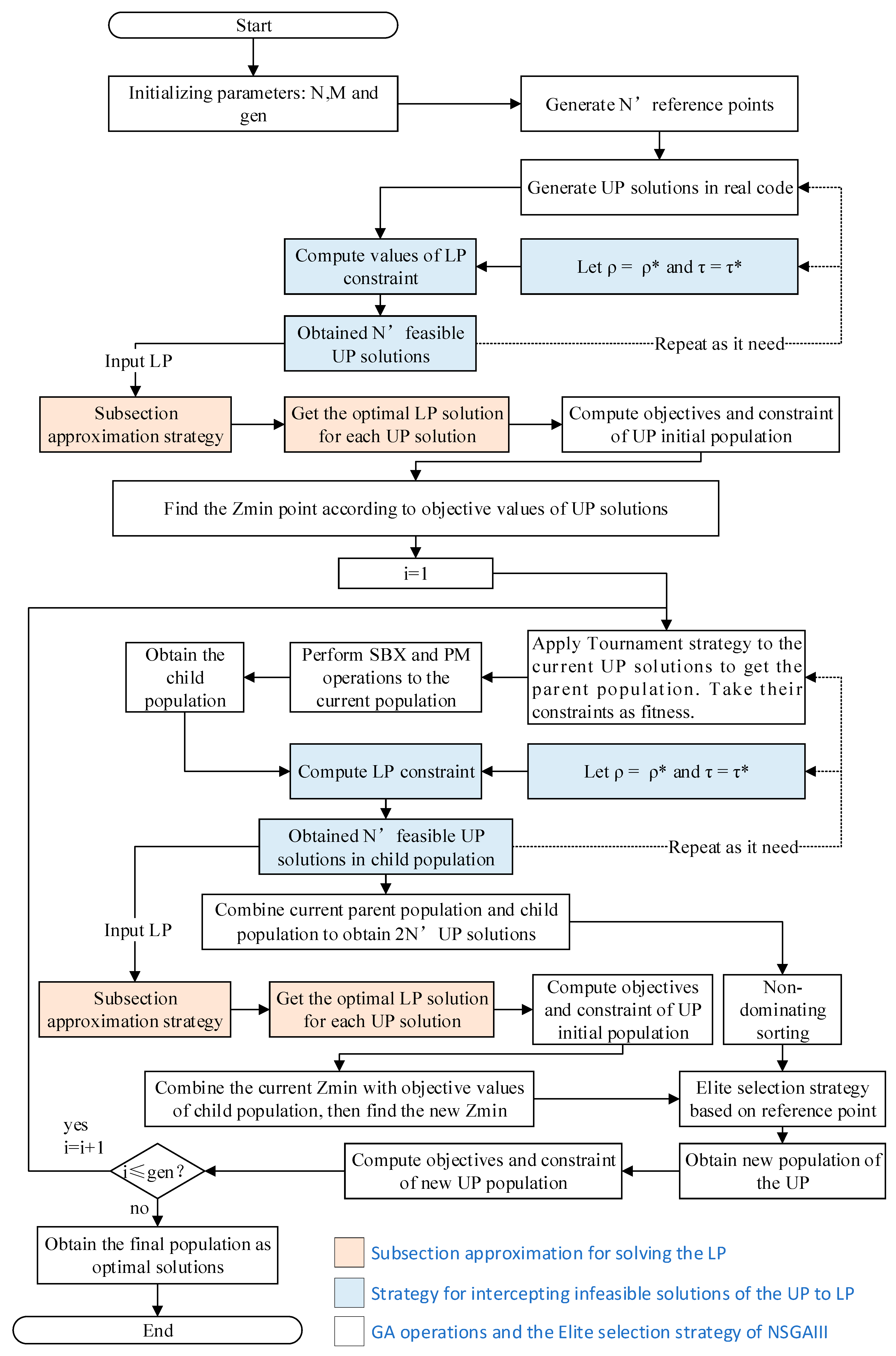
The entire process of the proposed algorithm for the built BLP model is implemented with the ‘PlatEMO’ [31] source code, including the following steps (Figure 5):

Step 0 Initialize the parameters of the NSGAIII algorithm. These parameters are population size $N$, the number of objective functions $M$ and the maximum generation times $\mathrm{gen}$. The actual size of population $N{}^{\prime }$ will be determined by the inherent reference point generation method of NSGAIII [32].

Step 1: Generate a population of $N{}^{\prime }$ individuals of $\left\{\alpha ,\delta ,\epsilon \right\}$ by real coding. In other words, generate $N{}^{\prime }$ random numbers between the upper limit and lower limit of each variable ($\alpha$, $\delta$ or $\epsilon$), then rearrange them as an $N{}^{\prime }\times 3$ matrix. Then, perform the interception strategy listed in Section 4.1 to obtain $N{}^{\prime }$ globally feasible solutions, where each of them is a combination of $\{\alpha ,\delta ,\epsilon ,p,\tau \}$.

Step 2: Calculate values of the UP problem’s objective functions with $N{}^{\prime }$ $\{\alpha ,\delta ,\epsilon ,p,\tau \}$ and find the minimum value for each objective to form the coordinate set $Z_{\min }$ of the “ideal point”. For example, each of $z_{\min }^{(1)}$, $z_{\min }^{(2)}$ and $z_{\min }^{(3)}$ is the minimum element of objective function 1, 2 and 3 of in the upper level; then, we find that $Z_{\min }=\{z_{\min }^{(1)},z_{\min }^{(2)},z_{\min }^{(3)}\}$.

Step 3: Generate $N{}^{\prime }$ parent individuals of $\left\{\alpha ,\delta ,\epsilon \right\}$ by the tournament selection strategy [33], then perform the Simulate Binary Crossover (SBX) [34] and Polynomial Mutation (PM) [35] operations to obtain the child population for the current epoch. Repeat the strategy listed in Section 4.1 with the tournament, SBX and PM operations as needed to make all child individuals available to solve the solutions of the LP.

Step 4: Combine the parent population and child population together to obtain 2$N{}^{\prime }$ individuals of $\{\alpha ,\delta ,\epsilon ,p,\tau \}$; then, calculate their objective functions as fitness.

Step 5: Perform the Effective Non-Dominating Sorting (ENS) strategy [36] on the 2$N{}^{\prime }$ individuals and allocate a non-dominating serial number to each individual. The elite selection strategy based on reference points [37] should be carried out for those individuals with the largest serial number.

Step 6: Repeat Step 3 to Step 5 until the maximum generation time $\mathrm{gen}$ is reached. The final population of individuals is taken as the Pareto solution set of the entire BLP.

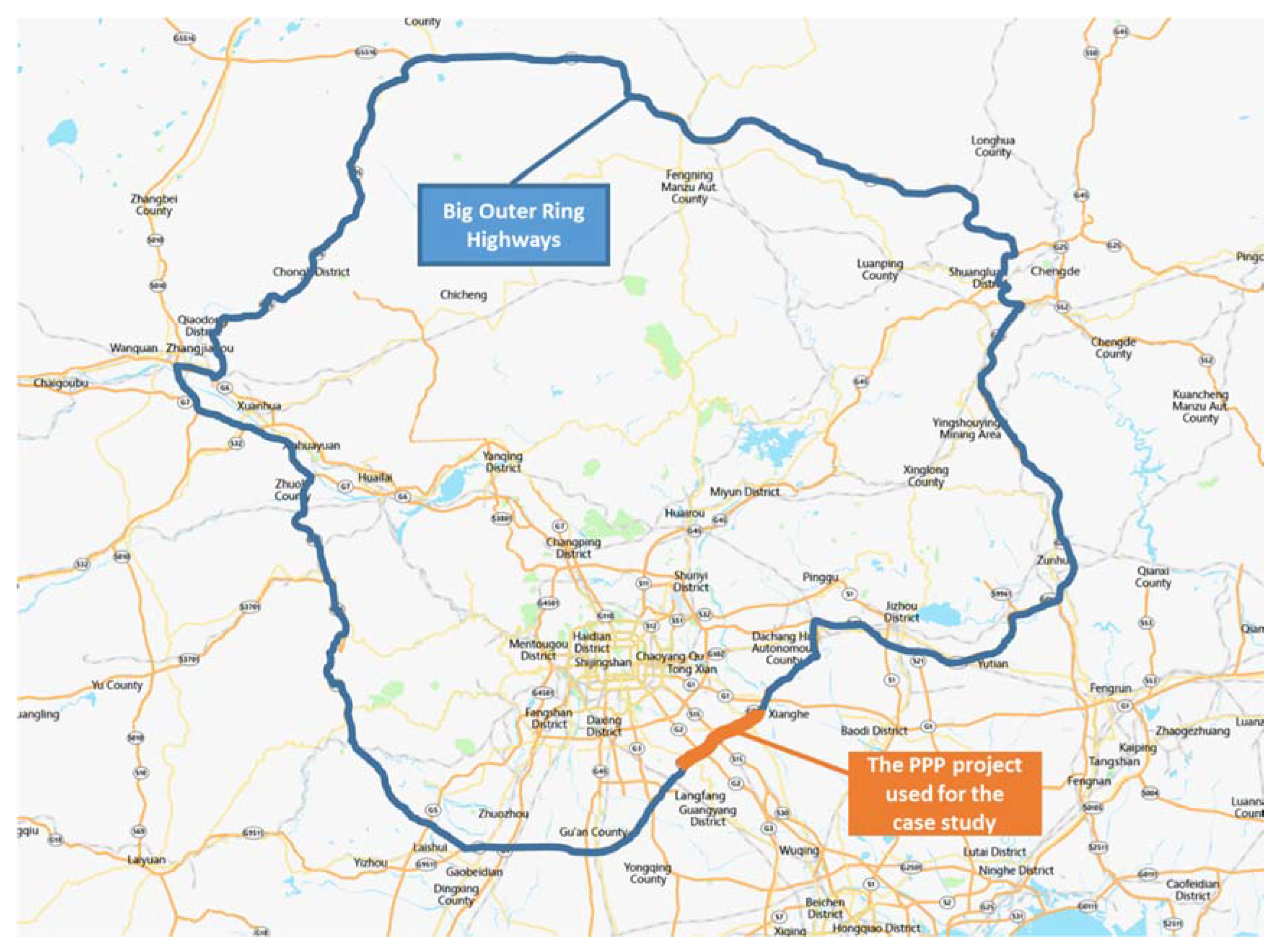
5. A case Study of the Big Outer Ring Highway PPP Project

5.1. The Big Outer Ring Highway PPP Project

According to the PPP implementation plan of the Big Outer Ring Highway (Figure 6), the total investment ($I$) is about 13.5 billion Yuan (1.94 billion USD at an exchange rate of 1:6.9501), the construction period is 2 years (2017–2018) and the operation period is 25 years (2019–2043). The capital fund ratio ($r^{\mathrm{cap}}$) is 25% of the total investment, and the project has been granted a sum of extra funding ($I{}^{\prime }$) from the central government equal to the amount of the capital funding. The interest rate of long-term loans for more than five years ($r^{\mathrm{deb}}$) is 4.9%. The expected ratio of non-toll income to toll income ($r_{\mathrm{nt}}$) is 2%. The least expected ROI of the private sector ($r^{\mathrm{pri}}$) is 8%, and the ROI of the public sector ($r^{\mathrm{gov}}$) is 4.25%. Other input parameters of the operation period are listed in

Table 1. Input parameters of the highway PPP project (in USD).

Year	Operation Subsidy in Original Case ($ Million)	$\mathbf{Traffic}{\mathit{q}}_{\mathit{i}}(\mathbf{Year},\mathbf{Million}-\mathbf{Vehicle})$	Unit Traffic Subsidy ($ Vehicle-km)	$\mathbf{Operation}\mathbf{Cos}\mathbf{t}{\mathit{c}}_{\mathit{i}}(\$\mathbf{Million})$	$\mathbf{Exterior}\mathbf{Benefit}\left(\mathbf{EB}\right){\mathit{e}}_{\mathit{i}}(\$\mathbf{Million})$
2019	24.22	231.49	0.10462	27.19	111.57
2020	30.65	292.94	0.10462	28.28	220.54
2021	38.78	370.70	0.10462	29.42	265.32
2022	49.08	469.10	0.10462	30.61	301.64
2023	62.11	593.63	0.10462	31.85	332.97
2024	66.79	634.72	0.10523	33.15	385.35
2025	71.42	678.65	0.10523	34.51	439.89
2026	76.36	725.63	0.10523	35.93	496.65
2027	81.65	775.85	0.10524	37.42	555.69
2028	87.30	829.55	0.10523	38.97	617.05
2029	87.62	845.48	0.10363	40.60	638.83
2030	89.30	861.71	0.10363	42.30	661.38
2031	91.01	878.26	0.10363	44.08	684.73
2032	92.76	895.12	0.10363	45.94	708.90
2033	94.54	912.30	0.10363	47.89	733.94
2034	94.47	920.81	0.10259	49.93	759.88
2035	95.35	929.39	0.10259	52.06	786.76
2036	96.23	938.05	0.10259	54.29	814.61
2037	97.13	946.80	0.10259	56.63	842.78
2038	98.04	955.62	0.10259	59.08	871.33
2039	97.41	964.53	0.10100	61.64	876.72
2040	98.32	973.52	0.10100	64.32	899.72
2041	99.24	982.60	0.10099	67.12	923.68
2042	100.16	991.75	0.10100	70.06	948.55
2043	101.09	1001.01	0.10099	73.14	974.45

.

The upper limit and lower limit of the decision variables are shown in

Table 2. Values of the upper limit and lower limit of decision variables.

	$\mathbf{Share}\mathbf{of}\mathbf{Equity}\mathbf{Fund}\mathit{\alpha }$ (%)	$\mathbf{Unit}\mathbf{Subsidy}\mathit{\delta }$ ($ Vehicle-km)	$\mathbf{Ratio}\mathbf{of}\mathbf{EB}\mathbf{Transferred}\mathit{\epsilon }$ (%)	$\mathbf{Unit}\mathbf{Toll}\mathit{\rho }$ ($ Vehicle-km)	$\mathbf{Concession}\mathbf{Term}\mathit{\tau }$ (Years)
Upper limit	${\alpha }^{\max }=49\%$	${\delta }^{\max }=0.10524$	$\epsilon =100\%$	$\rho =0.09928$	$\tau =25$
Lower limit	${\alpha }^{\min }=0\%$	${\delta }^{\min }=0$	$\epsilon =0\%$	$\rho =0$	$\tau =15$

. The upper limit of variable $\delta$ is determined according to the maximum unit traffic subsidy (shown in Table 2, column 4), while other values are extracted from the project plan report.

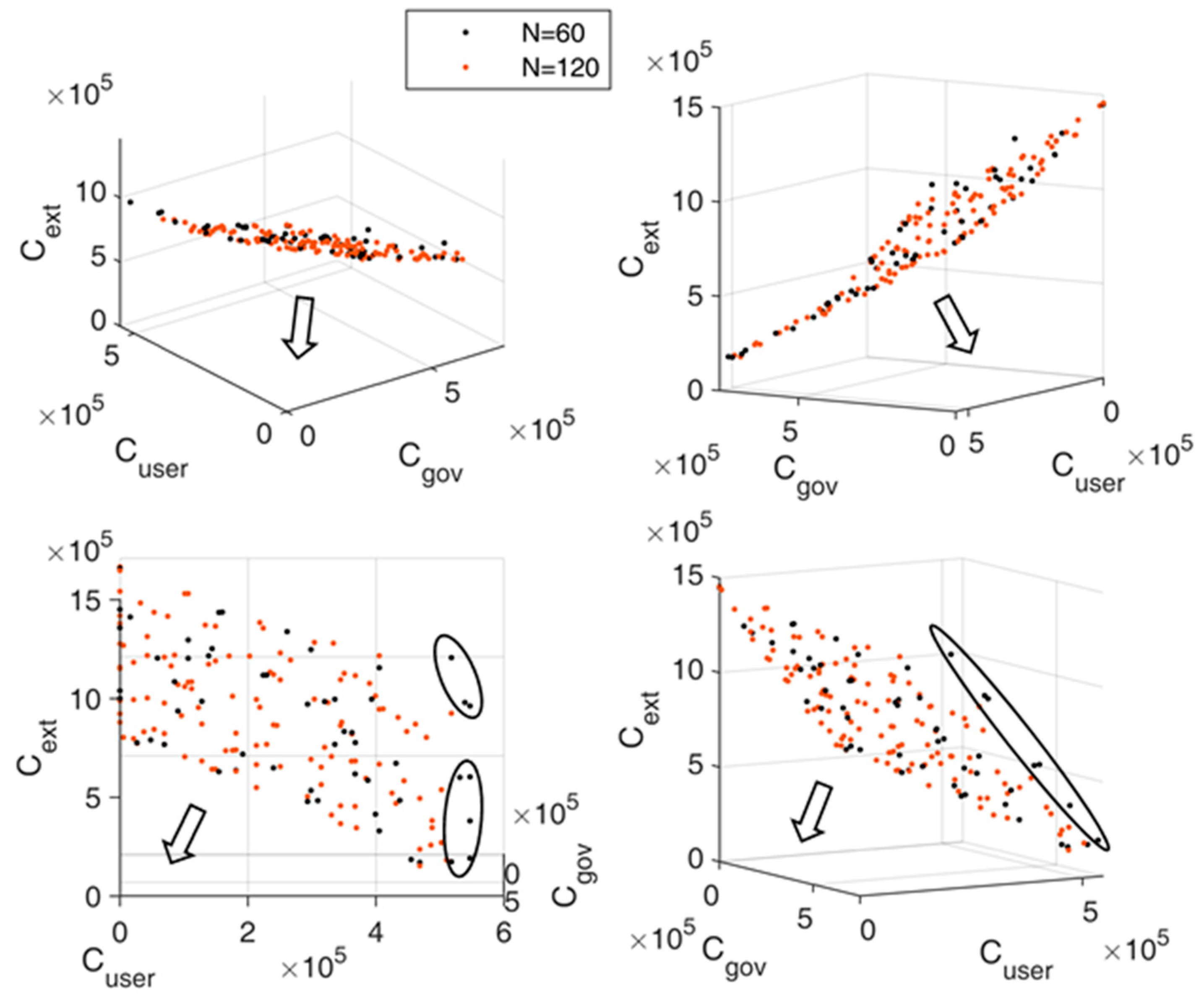
5.2. Evaluation Effects of Different Population Sizes

Population size is one of the key parameters of the non-dominating sorting GA algorithms. The effects of two population sizes $N=60$ and $N=120$ are compared with the NSGAIII algorithm. Figure 7 shows the distribution of the Pareto solutions of the two population sizes from different views in the three-dimensional space. Arrows point to the convergence direction. It can be seen from Figure 7 that the group of $N=120$ performs better in terms of the convergence and evenness of solutions. There are also some solutions of group $N=60$ that are relatively far away from the front edge (in the convergence direction) of the solution set, which means that these solutions are inferior to those that are right on or close to the front edge.

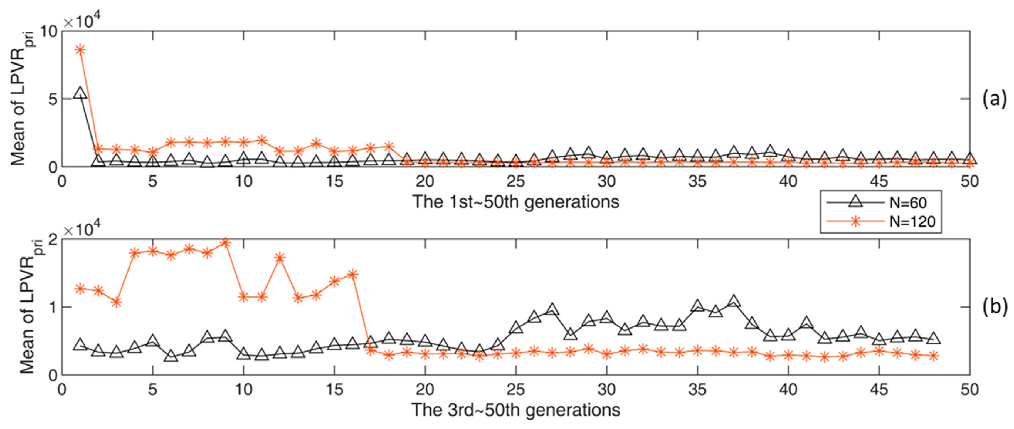
It can be seen from Figure 8a that a larger population creates better convergence, even though there is little difference between the two sizes of population in general. Values of the LP objective functions in the first two iterations are much higher than those in the subsequent iterations; thus, the convergence curve starts from the third to the 50th iteration, as shown independently in Figure 8b. It can be seen in Figure 8b that a larger population size leads to a better convergence than a smaller population size after the 17th iteration. Results of the group are kept for analysis in later sections of this paper.

5.3. Results and Discussion

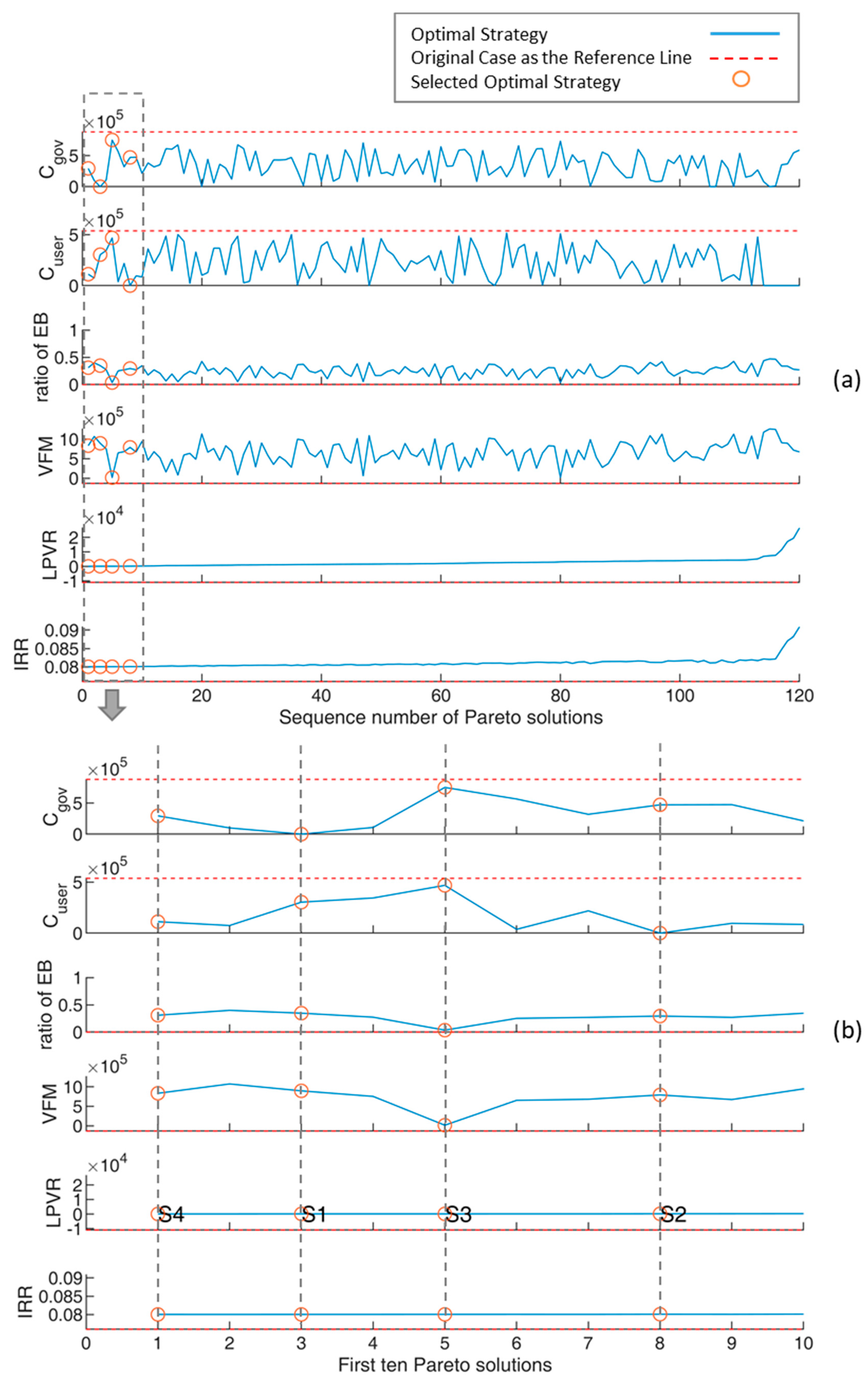
$C_{\mathrm{gov}}$, $C_{\mathrm{user}}$, $\epsilon$, VFM, LPVR and the private sector’s IRR for all the 120 Pareto solutions, arranged in the order of increasing LPVR values, are plotted as stacked lines in Figure 9a. From the 120 Pareto solutions, the optimal strategies for minimizing the costs of the public sector (S1), minimizing user payment (S2), minimizing the transferred exterior benefits (S3) and minimizing the LPVR of the private sector (S4) are drawn out separately in Figure 9b. For each type of optimal strategy, only the strategies which generated the lowest LPVR are chosen. In that case, all four optimal strategies are located within the range of the first 10 solutions.

It can be seen from Figure 9a that VFM and LPVR are both less than zero in the original case (the red dot lines), illustrating that strategies of the original case are not feasible for implementing the project via PPP. The ratio of consumed exterior benefits in all Pareto solutions is above that in the original case, which means the problem might be infeasible without transferring certain amounts of exterior benefits as supplementary income into the project. Variation of $C_{\mathrm{gov}}$ and of VFM are not linearly correlated, revealing their sum, i.e., the PSC value is not stable. Therefore, it is not appropriate to use the VFM value to evaluate different PPP strategies.

Table 3. Changes in decision variables.

	$\mathbf{Share}\mathbf{of}\mathbf{Equity}\mathbf{Fund}\mathit{\alpha }$ (%)	$\mathbf{Unit}\mathbf{Subsidy}\mathit{\delta }$ ($ Vehicle-km)	$\mathbf{Ratio}\mathbf{of}\mathbf{EB}\mathbf{Transferred}\mathit{\epsilon }$ (%)	$\mathbf{Unit}\mathbf{Toll}\mathit{\rho }$ ($ Vehicle-km)	$\mathbf{Concession}\mathbf{Term}\mathit{\tau }$ (Years)
S0	49.00%	0.1034	0.00%	0.0976	25
S1	0.00%	0.0000	34.71%	0.0820	15
Δ1	−49.00%	−100.00%	+34.71%	−15.94%	−40.00%
S2	48.22%	0.0726	29.43%	0.0000	15
Δ2	−0.78%	−29.84%	+29.43%	−100.00%	−40.00%
S3	47.30%	0.1035	3.55%	0.0993	20
Δ3	−1.70%	+0.05%	+3.55%	+1.75%	−20.00%
S4	45.05%	0.0344	30.93%	0.0302	15
Δ4	−3.95%	−66.69%	+30.93%	−69.03%	−40.00%

,

Table 4. Changes in indicators reflecting the benefits and costs of the public sector. PSC: public sector comparator. VFM: value for money.

	${\mathit{C}}_{\mathbf{gov}}$ ($ Million)	PSC ($ Million)	VFM ($ Million)	${\mathit{F}}_{\mathbf{gov}}^{\mathbf{equity}}$ ($ Million)	${\mathit{S}}_{{\mathit{r}}_{\mathbf{gov}}}$ ($ Million)
S0	1267.02	1071.83	−195.19	238.00	1043.38
S1	0.00	1289.00	1289.00	0.00	0.00
Δ1	−100.00%	+20.26%	+760.38%	−100.00%	−100.00%
S2	677.91	1816.86	1138.95	234.21	457.83
Δ2	−46.50%	+69.51%	+683.50%	−1.59%	−56.12%
S3	1080.09	1100.84	20.75	229.76	864.19
Δ3	−14.75%	+2.71%	+110.63%	−3.46%	−17.17%
S4	422.94	1622.39	1199.44	218.81	217.33
Δ4	−66.62%	+51.37%	+714.50%	−8.06%	−79.17%

and

Table 5. Change in indicators reflecting the benefits and costs of the private sector.

	LPVR ($ Million)	${\mathbf{irr}}_{\mathbf{pri}}$ (%)	${\mathit{R}}_{\mathbf{sub}}$ ($ Million)	${\mathit{R}}_{\mathbf{tol}}$ ($ Million)	${\mathit{R}}_{\mathbf{ext}}$ ($ Million)	${\mathit{F}}_{\mathbf{pri}}^{\mathbf{equity}}$ ($ Million)	${\mathit{C}}_{\mathbf{ope}}$ ($ Million)
S0	−15.82	7.60%	630.23	606.52	0.00	247.71	360.58
S1	0.20	8.00%	0.00	364.98	1054.59	485.71	253.18
Δ1	+101.26%	+0.40%	−100.00%	−39.82%	-	+96.08%	−29.78%
S2	0.29	8.01%	316.56	0.00	894.28	251.50	253.18
Δ2	+101.82%	+0.41%	−49.77%	−100.00%	-	+1.53%	−29.78%
S3	0.20	8.01%	556.02	544.19	138.90	255.95	311.51
Δ3	+101.29%	+0.41%	−11.78%	−10.28%	-	+3.32%	−13.61%
S4	0.13	8.00%	150.27	134.47	939.67	266.91	253.18
Δ4	+100.83%	+0.40%	−76.16%	−77.83%	-	+7.75%	−29.78%

separately show the changes when each optimal solution is compared with the original case solution (S₀) in different indicators. Their definitions are listed in

Table A2. Notations and definitions of parameters and variables used in Section 5.3. NPV: net present value.

Notation	Definition
$F_{\mathrm{gov}}^{\mathrm{equity}}$	NPV of the equity fund shared by the private sector
$S_{r_{\mathrm{gov}}}$	NPV of the equity fund shared by the public sector
$F_{\mathrm{pri}}^{\mathrm{equity}}$	NPV of the subsidy paid by the public sector as costs, discounted by $r_{\mathrm{gov}}$
${\mathrm{irr}}_{\mathrm{pri}}$	Internal return rate (IRR) of the private sector over the project’s life
$R_{\mathrm{sub}}$	NPV of the subsidy paid by the public sector and received by the private sector as revenue, discounted by $r_{\mathrm{pri}}$
$R_{\mathrm{tol}}$	NPV of toll collected by the private sector
$R_{\mathrm{ext}}$	NPV of the exterior benefits transferred and taken by the private sector as extra revenue
$C_{\mathrm{ope}}$	NPV of the operation costs paid by the private sector

of Appendix A. Δ₁~Δ₄ show the increments of S₁~S₄ when compared to S₀. Changes in $\alpha$, $\epsilon$, ${\mathrm{irr}}^{\mathrm{pri}}$ and $\tau$ are measured in absolute increments as:

$${\Delta }_i=S_i-S_0,i=1,2,3,4$$

(18)

Changes in $\delta$, $\rho$, $C_{\mathrm{gov}}$, PSC, VFM, $F_{\mathrm{gov}}^{\mathrm{equity}}$, $S_{r_{\mathrm{gov}}}$, and $B_{\mathrm{pri}}$,$R_{\mathrm{sub}}$,$R_{\mathrm{tol}}$, $F_{\mathrm{pri}}^{\mathrm{equity}}$ and $C_{\mathrm{ope}}$ are measured in relative increments as:

$${\Delta }_i=\frac{S_i-S_0}{S_0},i=1,2,3,4$$

(19)

The following discussion is based on the results shown in Table 3, Table 4 and Table 5.

S₁ offers a scheme of nearly complete privatization, which is without any capital fund or subsidy paid by the public sector. The results of S₁ reveal that the public sector can achieve maximum benefit when delivering the project in a fully market-based schema.

S₂ provides a schema equivalent to opening up the project to the public for free. Besides, adding 29.43% of exterior benefits realizes a 46.5% reduction in the public sector cost.

S₃ shows that at least 3.55% of exterior benefits need to be transferred into the project to meet the two prerequisites of PPP. In S3, the unit payment of users increases by 1.75% while the public sector cost reduces by 14.75%, which indicates that the strategy of minimum consumption of exterior benefits is more beneficial to the public sector than to users.

In S₄, the actual IRR of the private sector is almost the same as the other three optimal strategies. Compared with S₁, S₂ and S₃, S₄ provides a more balanced schema, in which the consumption of exterior benefits increases by 30.93%, the cost of the public sector reduces by 66.62% and the unit payment of users decreases by 69.03%.

It can be seen in all four optimal strategies that shortening the concession term plays the most critical role in cutting down the cost of the public sector and increasing the benefit of the private sector. Both parties benefit from the reduction of their own costs in the operation period.

6. Conclusions

This paper studies the problem of Stackelberg game optimization under an LPVR mechanism when negotiating a transport PPP project between the public sector and the private sector. The decision-making scenario and the characteristics of the Stackelberg game during procurement are described and analyzed. Based on that analysis, a BLP model is constructed. The objective of the UP problem is to minimize the costs, including the public sector cost and the user payment. The constraint of the UP is to realize value for money for the public sector. The objective of the LP problem is to minimize the difference between the actual returns and the expected returns of the private sector, and its constraint is that the actual returns must be no less than the expected level.

An intuitive algorithm based on the NSGAIII framework is designed to solve the BLP model. In order to generate global feasible solutions that satisfy both the UP and LP constraints, an interception strategy is carried out to avoid infeasible solutions from UP to LP. Based on the analysis of the objective function of the LP, a subsection approximating algorithm to solve the LP by discretizing variables of the concession term and toll is proposed.

The effectiveness of the model and algorithm is validated by the PPP project of the Beijing Big Outer Ring highway. Solutions maximizing each single objective are selected from the Pareto solution set. Costs and benefits for both the public sector and the private sector under different solutions are compared and discussed. Main findings include that (1) the PPP project will be financially infeasible without transferring certain amounts of exterior benefits into supplementary income for the private sector; (2) the strategy of transferring the minimum exterior benefits is more beneficial to the public sector than to users; (3) the public sector can achieve maximum benefit when delivering the project in a fully market-based schema; and (4) the value of VFM is not suitable for use as the evaluation criteria for PPP investment schemas since its computation base, the PSC, is not static.

It is necessary to know that results in this study are case-specific, as it has not been ensured that each project generates the same level of returns. This paper is models the Stackelberg decision-making problem of two parties only. In future research, the public, local residents, tax payers, pure investors and other stakeholders in PPPs could be involved, and a multi-layered Stackelberg MOP could be built to further simulate more complex decision-making scenarios.

References

- Wang, H.; Xiong, W.; Wu, G.; Zhu, D. Public-private partnership in public administration discipline: A literature review. Public Manag. Rev. 2018, 20, 293–316. [Google Scholar] [CrossRef]
- Koppenjan, J.J.F. The formation of public-private partnerships: Lessons from nine transport infrastructure projects in The Netherlands. Public Admin. 2005, 83, 135–157. [Google Scholar] [CrossRef]
- Papajohn, D.; Cui, Q.; Bayraktar, M.E. Public-private partnerships in US transportation: Research overview and a path forward. J. Manag. Eng. 2011, 27, 126–135. [Google Scholar] [CrossRef]
- Garvin, M.J. Enabling development of the transportation public-private partnership market in the United States. J. Constr. Eng. Manag. 2010, 136, 402–411. [Google Scholar] [CrossRef]
- Xu, Y.; Yeung, J.F.; Jiang, S. Determining appropriate government guarantees for concession contract: Lessons learned from 10 PPP projects in China. Int. J. Strateg. Prop. Manag. 2014, 18, 356–367. [Google Scholar] [CrossRef]
- Kayhan, İ.E.; Jenkins, G.P. Determination of socially equitable guarantees for public-private partnerships: A toll-road case from Turkey. Turkish Stud. 2016, 17, 691–711. [Google Scholar] [CrossRef]
- Rouhani, O.M.; Gao, H.O.; Geddes, R.R. Policy lessons for regulating public-private partnership tolling schemes in urban environments. Transp. Policy 2015, 41, 68–79. [Google Scholar] [CrossRef]
- Song, J.; Zhao, Y.; Jin, L.; Sun, Y. Pareto optimization of public-private partnership toll road contracts with government guarantees. Transp. Res. Part A Policy Pract. 2018, 117, 158–175. [Google Scholar] [CrossRef]
- Button, K.; Daito, N. Sharing out the costs of a public-private partnership. Appl. Econ. Lett. 2014, 21, 383–386. [Google Scholar] [CrossRef]
- Vassallo, J.M. The role of the discount rate in tendering highway concessions under the LPVR approach. Transp. Res. Part A Policy Pract. 2010, 44, 806–814. [Google Scholar] [CrossRef] [Green Version]
- Peng, W.; Cui, Q.; Chen, J. Option game model for optimizing concession length and public subsidies of public-private partnerships. Transp. Res. Rec. 2014, 109–117. [Google Scholar] [CrossRef]
- Liu, T.; Bennon, M.; Garvin, M.J.; Wang, S. Sharing the big risk: Assessment framework for revenue risk sharing mechanisms in transportation public-private partnerships. J. Constr. Eng. Manag. 2017, 143. [Google Scholar] [CrossRef] [Green Version]
- Sharafi, A.; Taleizadeh, A.A.; Amalnicka, M.S. Fair allocation in financial disputes between public-private partnership stakeholders using game theory. Serv. Sci. 2018, 10, 1–11. [Google Scholar] [CrossRef]
- South, A.; Eriksson, K.; Levitt, R. How Infrastructure public-private partnership projects change over project development phases. Proj. Manag. J. 2018, 49, 62–80. [Google Scholar] [CrossRef]
- Engel, E.; Fischer, R.; Galetovic, A. Privatizing Roads: A New Method for Auctioning Highways; The World Bank Group: Washington, DC, USA, 1997. [Google Scholar]
- Rouhani, O.M.; Geddes, R.R.; Do, W.; Gao, H.O.; Beheshtian, A. Revenue-risk-sharing approaches for public-private partnership provision of highway facilities. Case Stud. Transp. Policy 2018, 6, 439–448. [Google Scholar] [CrossRef]
- Engel, E.M.; Fischer, R.D.; Galetovic, A. Least-present-value-of-revenue auctions and highway franchising. J. Polit. Econ. 2001, 109, 993–1020. [Google Scholar] [CrossRef] [Green Version]
- Sharma, R.; Newman, P. Can land value capture make PPP’s competitive in fares? A Mumbai case study. Transp. Policy 2018, 64, 123–131. [Google Scholar] [CrossRef] [Green Version]
- Chen, C.L.; Cruz, J. Stackelburg solution for two-person games with biased information patterns. IEEE Trans. Automat. Control 1972, 17, 791–798. [Google Scholar] [CrossRef] [Green Version]
- Yang, H.; Bell, M.G.; Meng, Q. Modeling the capacity and level of service of urban transportation networks. Transp. Res. Part B Methodol. 2000, 34, 255–275. [Google Scholar] [CrossRef]
- Gao, Z.; Zhang, H.; Sun, H. Bi-level programming models, approaches and applications in urban transportation network design problems. Commun. Transp Syst. Eng. Inf. 2004, 4, 35–44. [Google Scholar]
- Liu, F.; Liu, J.; Yan, X. Quantifying the decision-making of PPPs in China by the entropy-weighted pareto front: A URT case from Guizhou. Sustainability 2018, 10, 1753. [Google Scholar] [CrossRef] [Green Version]
- Roghanian, E.; Aryanezhad, M.; Sadjadi, S.J. Integrating goal programming, Kuhn-Tucker conditions, and penalty function approaches to solve linear bi-level programming problems. Appl. Math. Comput. 2008, 195, 585–590. [Google Scholar] [CrossRef]
- Zhou, J.; Lam, W.H. A bi-level programming approach—Optimal transit fare under line capacity constraints. J. Adv. Transp. 2001, 35, 105–124. [Google Scholar] [CrossRef]
- Shang, L.; Aziz, A.M.A. Stackelberg game theory-based optimization model for design of payment mechanism in performance-based PPPs. J. Constr. Eng. Manag. 2020, 146. [Google Scholar] [CrossRef]
- Zhang, L.; Feng, X.; Chen, D.; Zhu, N.; Liu, Y. Designing a hazardous materials transportation network by a bi-level programming based on toll policies. Phys. A 2019, 534. [Google Scholar] [CrossRef]
- Jia, X.; He, R.; Zhang, C.; Chai, H. A Bi-level programming model of liquefied petroleum gas transportation operation for urban road network by period-security. Sustainability 2018, 10, 4714. [Google Scholar] [CrossRef] [Green Version]
- Assadipour, G.; Ke, G.Y.; Verma, M. A toll-based bi-level programming approach to managing hazardous materials shipments over an intermodal transportation network. Transp. Res. D Transp. Environ. 2016, 47, 208–221. [Google Scholar] [CrossRef]
- Fleming, P.J.; Purshouse, R.C.; Lygoe, R.J. Many-Objective Optimization: An Engineering Design Perspective; Springer: Berlin/Heidelberg, Germany, 2005; pp. 14–32. [Google Scholar]
- Tian, Y.; Xiang, X.; Zhang, X.; Cheng, R.; Jin, Y. Sampling Reference Points on the Pareto Fronts of Benchmark Multi-Objective Optimization Problems; IEEE: Piscataway, NJ, USA, 2018; pp. 1–6. [Google Scholar]
- Tian, Y.; Cheng, R.; Zhang, X.; Jin, Y. PlatEMO: A MATLAB platform for evolutionary multi-objective optimization. IEEE Comput. Intell. Manag. 2017, 12, 73–87. [Google Scholar] [CrossRef] [Green Version]
- Deb, K.; Jain, H. An evolutionary many-objective optimization algorithm using reference-point-based nondominated sorting approach, part I: Solving problems with box constraints. IEEE Trans. Evolut. Comput. 2013, 18, 577–601. [Google Scholar] [CrossRef]
- Das, I.; Dennis, J.E. Normal-boundary intersection: A new method for generating the Pareto surface in nonlinear multicriteria optimization problems. SIAM J. Optimiz. 1998, 8, 631–657. [Google Scholar] [CrossRef] [Green Version]
- Yang, J.; Soh, C.K. Structural optimization by genetic algorithms with tournament selection. J. Comput. Civil Eng. 1997, 11, 195–200. [Google Scholar] [CrossRef]
- Deb, K.; Agrawal, R.B. Simulated binary crossover for continuous search space. Complex. Syst. 1995, 9, 115–148. [Google Scholar]
- Kumar, S.; Naresh, R. Nonconvex economic load dispatch using an efficient real-coded genetic algorithm. Appl. Soft Comput. 2009, 9, 321–329. [Google Scholar] [CrossRef]
- Zhang, X.; Tian, Y.; Cheng, R.; Jin, Y. An efficient approach to nondominated sorting for evolutionary multiobjective optimization. IEEE Trans. Evolut. Comput. 2014, 19, 201–213. [Google Scholar] [CrossRef] [Green Version]
Figure 1.
The technology roadmap of the study in this paper. PPP: public-private partnership; LPVR: least present value of revenue.
Figure 2.
An interactive decision-making process in a PPP project context initialized by the public sector as the leader.
Figure 3.
How the objectives of the upper programing (UP) problem and the lower programing (LP) problem are optimized.
Figure 4.
Surface diagram with contours of the functional relationships between , and . and .
Figure 5.
Process of the entire algorithm used to solve the complete bi-level programing (BLP) model. NSGAIII: non-dominated sorting genetic algorithm III.
Figure 6.
Sketch of the location of the Big Outer Ring Highways on a plain map.
Figure 7.
The distribution of the LP problem’s objective values, calculated by two sizes of population under the NSGAIII algorithm. Three objectives of the UP problem are shown, which are the lifecycle cost of the public sector (), user payment (), and the consumption of exterior benefit ().
Figure 8.
The convergence of the LP problem’s objective values calculated by two sizes of population under the NSGAIII algorithm. (a) shows convergence of all 50 generations, and (b) shows convergence of the 3rd–50th generations.
Figure 9.
The convergence of the LP problem’s objective values calculated by two sizes of population under NSGAIII algorithm. (a) shows the stacked plot of all 120 solutions with a dashed box outlining the general locations of those selected optimal solutions. (b) displays contents in the dashed box of (a), and each dashed line represents one selected optimal solution.