Omnidirectional Mobile Robot Dynamic Model Identification by NARX Neural Network and Stability Analysis Using the APLF Method

Abstract

In this paper, the NARX neural network system is used to identify the complex dynamics model of omnidirectional mobile robot while rotating with moving, and analyze its stability. When the mobile robot model rotates and moves at the same time, the dynamic model of the mobile robot is complex and there is motion coupling. The change of the model in different states is a kind of symmetry. In order to solve the problem that there is a big difference between the mechanism modeling motion simulation and the actual data, the dynamic model identification of mobile robot in special state based on NARX neural network is proposed, and the stability analysis method is given. To verify that the dynamic model of NARX identification is consistent with that of the mobile robot, the Activation Path-Dependent Lyapunov Function (APLF) algorithm is used to distinguish the NARX neural network model expressed by LDI. However, the APLF method needs to calculate a large number of LMIs in practice and takes a lot of time, and, to solve this problem, an optimized APLF method is proposed. The experimental results verify the effectiveness of the theoretical method.

1. Introduction

The omnidirectional mobile robot has more flexible mobile performance than the traditional wheeled mobile robot. Integration of electronic, mechanical, control, automation and communication technology, combined with the theoretical expertise of many professionals. It has wide application prospects in commercial, military, and civilian applications and has become an important research platform in the control field. Obstacle avoidance, path planning and visual image processing are also important research directions for omnidirectional mobile robots. How to improve robot control performance and model accuracy is one of the main foci in the field of the omnidirectional mobile robot. So, establishing an accurate dynamic model of a mobile robot is very helpful to the establishment of the accurate mobile robot control system [1,2,3,4,5,6].

There are many kinds of wheel arrangement for omnidirectional mobile robot and different arrangement will lead to different results of kinematic model and dynamic model [7,8]. At present, the main method is to use three omnidirectional wheels with 120-degree angle distribution, which takes into account the stability and reliability, reduces the use of mechanical components and the cost [9]. Good control effect and accurate model building are inseparable. Sira proposed a generalized proportional integral (GPI) observer to observe the uncertainty of omnidirectional mobile robot and compensate the control [10]. Ren discusses the influence of unknown friction on the dynamic model of a three-wheeled omnidirectional mobile robot [11]. A dynamic model control method based on a mobile robot is introduced, and the Lyapunov function is used to prove the asymptotic stability of the system [12]. However, when the model cannot be accurately established or the model is not accurate, it is a good solution to use NARX neural network to identify the system and design the corresponding controller [13]. For modeling and recognizing the dynamics model of 2-axis PAM robot, Anh proposed a forward dynamic MIMO neural network NARX model [14]. To identify the nonlinear model of small unmanned helicopter from experimental flight data, Tijani proposed a multiobjective differential evolution (MODE) method based on NARX neural network [15].

In order to analyze the stability of neural network system, Tanaka point out that the dynamics of neural network systems can be represented by a class of nonlinear systems treated as linear differential inclusions (LDI) [16,17,18], then, the Lyapunov equation is established to analyze the stability of the system. The quadratic form of common Lyapunov function (CLF) is usually used to analyze the stability of nominal linear systems [19]. However, the conservatism of CLF in stability analysis is still too high, therefore, a parameter-dependent Lyapunov function (PDLF) method is proposed, which greatly reduces the conservatism of the stability results, and is widely used as a reliable stability criterion [20,21,22,23]. In the following development, a k-sample variation method has been paid more and more attention by scholars [24,25,26]. Tognetti proposed a quadratic Lyapunov function based on current and past time information to analyze the stability of TS fuzzy system [27]. Xiang adds the uncertain parameters with a memory of a certain interval, which could reduce the conservativeness [28]. However, in application, as the number of system matrices A increases, the number of LMIs required to calculate the Lyapunov function also increases exponentially. Therefore, it is particularly important to reduce the use of the LDI method to represent the A matrices generated by the neural network system [16] and to reduce the number of LMIs that need to be calculated [29].

The work of this paper has three main points. Firstly, establishes the dynamic model of the omnidirectional mobile robot and introduces the NARX neural network to identify the condition that the dynamic model cannot accurately describe the actual movement state of the robot when the mobile robot moving with rotation. Secondly, a novel Activation Path-Dependent Lyapunov Function (APLF) method is introduced, which is used to analyze the neural network system represented by LDI. Finally, in order to solve the problem that a large number of LMIs need to be calculated when the step interval is too large in APLF method. An optimized APLF method to discuss the substitution of all LMI by a subset of vertex sequence is introduced. This paper is organized as follows: Section 2 establishes the dynamic model of omnidirectional mobile robot. Section 3 introduces NARX neural network to identify the state of rotation and movement of omnidirectional mobile robot. Section 4 introduces the LDI method to represent the identified NARX neural network. Presents the PR method to find the minimum representation in the set of LDI matrices, and introduces the APLF method to analyse the stability of the NARX neural network system. An optimized APLF method, which reduces the number of LMI and calculation time, is given in Section 5. Conclusions are provided in Section 6.

2. Omnidirectional Mobile Robot Model

2.1. Robot Kinematic Model

First the omnidirectional mobile robot coordinate system is established, which is divided into the global coordinate system and the robot body coordinate system [30]. The global coordinate system is the coordinate system of the world where the robot is located, and the relative position of the robot and the coordinate system in the body coordinate system is always constant. The robot coordinate frame is shown in Figure 1.

Where $y,x,o$ constitute the global coordinate system and $Y,O,X$ constitute the robot body coordinate system. $V_a,V_b,V_c$ are the rotational speed of the omnidirectional mobile robot drive wheel $T_1,T_2,T_3$ and the angle between them is $\phi =120$°. The speed of the omnidirectional mobile robot in the X direction and Y direction of the body coordinate system are respectively $V_X,V_Y$, the horizontal distance from the center point of the robot to the omnidirectional wheel is L. Define the angle between the robot carrier coordinate system and the world coordinate system is $\theta$, the rotation angular velocity is $\dot{\theta }$, and the counterclockwise direction is the positive direction. From the Figure 1, it can be seen that the kinematic equations of the three driving wheels of the mobile robot are:

$$\left[\begin{array}{c}{V}_a\\ V_b\\ V_c\end{array}\right]=\left[\begin{array}{ccc}-1& 0& L\\ cos\phi & -sin\phi & L\\ cos\phi & sin\phi & L\end{array}\right]\left[\begin{array}{c}{V}_X\\ V_Y\\ \dot{\theta }\end{array}\right]$$

(1)

Let the rotation matrix from the body coordinate system to the globle coordinate system be:

$$R=\left[\begin{array}{ccc}cos\theta & -sin\theta & L\\ sin\theta & cos\theta & L\\ 0& 0& 1\end{array}\right]$$

(2)

Then the x and y speed in the globle coordinate system are $V_{xg},V_{yg}$ and can be converted as follow:

$$\left[\begin{array}{c}{V}_{xg}\\ V_{yg}\\ \dot{\theta }\end{array}\right]=\left[\begin{array}{ccc}cos\theta & -sin\theta & L\\ sin\theta & cos\theta & L\\ 0& 0& 1\end{array}\right]\left[\begin{array}{c}{V}_X\\ V_Y\\ \dot{\theta }\end{array}\right]$$

(3)

It can be obtained from (1) and (3)

$$\left[\begin{array}{c}{V}_a\\ V_b\\ V_c\end{array}\right]=\left[\begin{array}{ccc}-cos\theta & -sin\theta & L\\ cos\phi cos\theta +sin\phi sin\theta & cos\phi sin\theta -sin\phi cos\theta & L\\ cos\phi cos\theta -sin\phi sin\theta & cos\phi sin\theta +sin\phi cos\theta & L\end{array}\right]\left[\begin{array}{c}{V}_{xg}\\ V_{yg}\\ \dot{\theta }\end{array}\right]$$

(4)

Equation (4) is the kinematic model of mobile robot. The input value $\left[V_{xg},V_{yg},\dot{\theta }\right]$ are the speed of Y,X axis and robot angular velocity in the globle coordinate system. The output volue $V_a,V_b,V_c$ are the target speed of three driving wheels of robot.

2.2. Robot Dynamic Model

The displacement and rotation angle of the mobile robot in global coordinate system are recorded as $q={\left[xy\theta \right]}^T$, Then the velocity vector is $\dot{q}={\left[\dot{x}\dot{y}\dot{\theta }\right]}^T$. Define $V_X=V_{xg},V_Y=V_{yg}$, the new vector is $V_M={\left[V_X{V}_Y\dot{\theta }\right]}^T$. Furthermore, $T_i(i=1,2,3)$ represents the traction force generated by each driving wheel. The force $F_x,F_y$ are the traction force applied to the center of gravity of the omnidirectional robot. The relationship between these two groups of forces is as follows:

$$\left\{\begin{array}{c}\hfill F_X=-T_1+\frac{1}{2}{T}_2+\frac{1}{2}{T}_3\\ \hfill F_Y=-\frac{\sqrt{3}}{2}{T}_2+\frac{\sqrt{3}}{2}{T}_3\\ \hfill M_I=L{T}_1+L{T}_2+L{T}_3\end{array}\right.$$

(5)

According to Newton’s second law, the formula of the rotational moment as follows:

$$\left\{\begin{array}{c}\hfill m({\dot{V}}_X-V_Y\dot{\theta })=F_X\\ \hfill m({\dot{V}}_Y-V_X\dot{\theta })=F_Y\\ \hfill I_v\ddot{\theta }=M_I\end{array}\right.$$

(6)

where $M_I$ is the moment of force around the axis of the robot gravity center. Equations (5) and (6) can be rewritten as:

$$\left[\begin{array}{ccc}\mathrm{m}& 0& 0\\ 0& \mathrm{m}& 0\\ 0& 0& {\mathrm{I}}_{\mathrm{v}}\end{array}\right]\left[\begin{array}{c}{\dot{\mathrm{V}}}_{\mathrm{X}}\\ {\dot{\mathrm{V}}}_{\mathrm{Y}}\\ \ddot{\theta }\end{array}\right]+\left[\begin{array}{ccc}0& -m\dot{\theta }& 0\\ m\dot{\theta }& 0& 0\\ 0& 0& 0\end{array}\right]\left[\begin{array}{c}{\mathrm{V}}_{\mathrm{X}}\\ {\mathrm{V}}_{\mathrm{Y}}\\ \dot{\theta }\end{array}\right]=\left[\begin{array}{ccc}-1& \frac{1}{2}& \frac{1}{2}\\ 0& -\frac{\sqrt{3}}{2}& \frac{\sqrt{3}}{2}\\ \mathrm{L}& \mathrm{L}& \mathrm{L}\end{array}\right]\left[\begin{array}{c}{\mathrm{T}}_1\\ {\mathrm{T}}_2\\ {\mathrm{T}}_3\end{array}\right]$$

(7)

Equation (7) is recorded as

$$M_I{\dot{V}}_M+C_1{V}_M=B_{1}T$$

(8)

It is known from (8) that if the mobile robot is to run at a certain speed and in a certain direction, the omnidirectional wheel must generate a certain torque, which requires a motor connected to the omnidirectional wheel to achieve. The dynamic equation for constructing a DC motor is:

$$I_0\dot{\omega }+\left(b_0+\frac{K_t{K}_b}{R_a}\right)\omega +\frac{r}{n}T=\frac{K_t}{R_a}u$$

(9)

Vector $u={\left[u_1{u}_2{u}_3\right]}^T$ is Input voltage for three DC motors, $\omega ={\left[{\omega }_1{\omega }_2{\omega }_3\right]}^T$ is the motor angular rate. In actual system, the motor needs to pass through a set of reduction gears to connect to the wheels. Let $\varphi ={\left[\varphi \varphi \varphi \right]}^T$ be the output speed of the DC motor after passing through the reduction gear set, which is the wheel speed. So the relationship between $\omega$ and $\varphi$ are:

$$\omega =n\varphi ,\varphi =\frac{1}{r}{\mathrm{J}}_{\mathrm{M}}{\mathrm{V}}_{\mathrm{M}}$$

(10)

where

$${\mathrm{J}}_{\mathrm{M}}=\left[\begin{array}{ccc}-1& 0& L\\ \frac{1}{2}& -\frac{\sqrt{3}}{2}& L\\ \frac{1}{2}& \frac{\sqrt{3}}{2}& L\end{array}\right]$$

Combining (9) and (10):

$$T=\frac{n}{r}(\frac{K_t}{R_a}u-I_0\frac{n}{r}{J}_M{\dot{V}}_M-\left(b_0+\frac{K_t{K}_b}{R_a}\right)\frac{n}{r}{J}_M{V}_M)$$

(11)

By combining (4) and (11), the dynamic model of omnidirectional mobile robot in body coordinate system is obtained as:

$$\left(M_1+\frac{I_0{n}^2}{r^2}{B}_1{J}_M\right){\dot{V}}_M+\left(C_1+\frac{n^2}{r^2}\left(b_0+\frac{K_t{K}_b}{R_a}\right)B_1{J}_M\right)V_M=\frac{K_{t}n}{r{R}_a}{B}_{1}u$$

(12)

It can be seen that before the (12), only the relationship between speed and force was studied, and the actual voltage value was not involved. However, the controller is ultimately controlled by exerting a control force on the motor, that is, the voltage. After the (12), the relationship between the control voltage of DC motor and the speed vector of mobile robot is clarified. Equation (12) can be rewritten as:

$$M_2{\dot{V}}_M+C_2{V}_M=B_{2}u$$

(13)

where

$$\begin{array}{cc}\hfill {\mathrm{M}}_2=& {\mathrm{M}}_1+\frac{{\mathrm{I}}_0{n}^2}{{\mathrm{r}}^2}{\mathrm{B}}_1{\mathrm{J}}_{\mathrm{M}},{\mathrm{C}}_2={\mathrm{C}}_1+\frac{{\mathrm{n}}^2}{{\mathrm{r}}^2}\left({\mathrm{b}}_0+\frac{{\mathrm{K}}_{\mathrm{t}}{\mathrm{K}}_{\mathrm{b}}}{{\mathrm{R}}_{\mathrm{a}}}\right){\mathrm{B}}_1{\mathrm{J}}_{\mathrm{M}}\hfill \\ \hfill B_2=& \frac{K_{t}n}{\mathrm{r}{\mathrm{R}}_a}{B}_1,P=\frac{n^2}{r^2}\left(b_0+\frac{K_t{K}_b}{R_a}\right)\hfill \end{array}$$

The velocity vector $\dot{q}={\left[\dot{x}\dot{y}\dot{\theta }\right]}^T$ in the global coordinate system has the following relationship with the velocity vector $V_M={\left[V_X{V}_Y\dot{\theta }\right]}^T$ in the body coordinate system:

$$\dot{q}=R{V}_M$$

(14)

Derivative (10) into:

$$\ddot{q}=\dot{R}{V}_M+R{\dot{V}}_M$$

(15)

Substituting (14) and (15) into Formula (13), we get:

$$M_2{R}^T\ddot{q}+\left(C_2{R}^T-M_2{R}^T\dot{R}{R}^T\right)\dot{q}=B_{2}u$$

(16)

Equation (16) can be rewritten as:

$$M_3\ddot{q}+C_3\dot{q}=B_{2}u$$

(17)

where

$$M_3=M_2{R}^T,C_3=C_2{R}^T-M_2{R}^T\dot{R}{R}^T$$

According to (17), set $\mathit{X}=\dot{q}$, then the final state space expression can be established:

$$\left\{\begin{array}{c}\dot{\mathit{X}}=-{M_3}^{-1}{C}_3\mathit{X}+{M_3}^{-1}{B}_{2}u\hfill \\ y=E_{3X3}\mathit{X}\hfill \end{array}\right.$$

(18)

Expand the vector $\mathit{X}$ we can get:

$$\left\{\begin{array}{c}\left[\begin{array}{c}\ddot{x}\\ \ddot{y}\\ \ddot{\theta }\end{array}\right]=\mathrm{A}\left[\begin{array}{c}\dot{x}\\ \dot{y}\\ \dot{\theta }\end{array}\right]+\mathrm{B}\left[\begin{array}{c}{u}_1\\ u_2\\ u_3\end{array}\right]\hfill \\ y=E_{3X3}\left[\begin{array}{c}\dot{x}\\ \dot{y}\\ \dot{\theta }\end{array}\right]\hfill \end{array}\right.$$

where

$$A=-{M_3}^{-1}{C}_3=\frac{-1}{\frac{3I_0{n}^2}{2r^2}+m}\left[\begin{array}{ccc}\frac{3}{2}P& \frac{3I_0{n}^2}{2r^2}\dot{\theta }& 0\\ -\frac{3I_0{n}^2}{2r^2}\dot{\theta }& \frac{3}{2}P& 0\\ 0& 0& \frac{3P{L}^2\left(\frac{3I_0{n}^2}{2r^2}+m\right)}{I_v+\frac{3I_0{n}^2{L}^2}{r^2}}\end{array}\right]$$

$$B={M_3}^{-1}{B}_2=\frac{\frac{K_{t}n}{r{R}_a}}{\frac{3I_0{n}^2}{2r^2}+m}\left[\begin{array}{ccc}-cos\theta & \frac{1}{2}cos\theta +\frac{\sqrt{3}}{2}sin\theta & \frac{1}{2}cos\theta -\frac{\sqrt{3}}{2}sin\theta \\ -sin\theta & \frac{1}{2}sin\theta -\frac{\sqrt{3}}{2}cos\theta & \frac{1}{2}sin\theta +\frac{\sqrt{3}}{2}cos\theta \\ \frac{\frac{3I_0{n}^2}{2r^2}+m}{\frac{K_{t}n}{r{R}_a}}L& \frac{\frac{3I_0{n}^2}{2r^2}+m}{\frac{K_{t}n}{r{R}_a}}L& \frac{\frac{3I_0{n}^2}{2r^2}+m}{\frac{K_{t}n}{r{R}_a}}L\end{array}\right]$$

Finally, a dynamic model of the three-wheeled omnidirectional mobile robot is established. The input of the model is the voltage $u={\left[u_1{u}_2{u}_3\right]}^T$ of the three motors, and the output is the speed vector $\dot{q}={\left[\dot{x}\dot{y}\dot{\theta }\right]}^T$ of the omnidirectional mobile robot in the global coordinate system. And the constant coefficients involved in matrix A and matrix B are given in

Table 1. Robot Mechanical Constants.

Parameter	Parameter Description	Value
m	Robot mass	10 kg
$R_a$	Motor armature resistance	1.2 $\Omega$
L	Wheel to robot centroid distance	0.17 m
r	Wheel radius	0.05 m
$I_0$	Wheel inertia	1.5 × 10${}^{-5}$ kg·m${}^2$
$I_v$	Robot inertia	0.125 kg·m${}^2$
$K_b$	Motor back EMF	460 r·min/V
$K_t$	Motor torque	0.025 N·m/A
n	Gear reduction ratio	27

.

An interesting fact is that when the mobile robot is moving normally without rotating, the simulation data of its dynamic model is consistent with the actual situation. However, when the mobile robot moves while rotating, $\theta$ and $\dot{\theta }$ will always change. At this time, the simulation data of the dynamic model cannot accurately describe the mobile robot.

Figure 2 shows that the omnidirectional mobile robot moves a 2 m × 2 m square trajectory at the speed of 0.5 (m/s) with a rotational angular velocity of 2 (rad/s). It can be seen that the dynamic model cannot accurately reflect the actual state of motion when the mobile robot is rotating with moving. The following will introduce using NARX neural network to identify the dynamic model of the mobile robot when it moving with rotating.

3. Using NARX Neural Network to Identify Dynamic Model

3.1. Introduction to NARX Neural Network

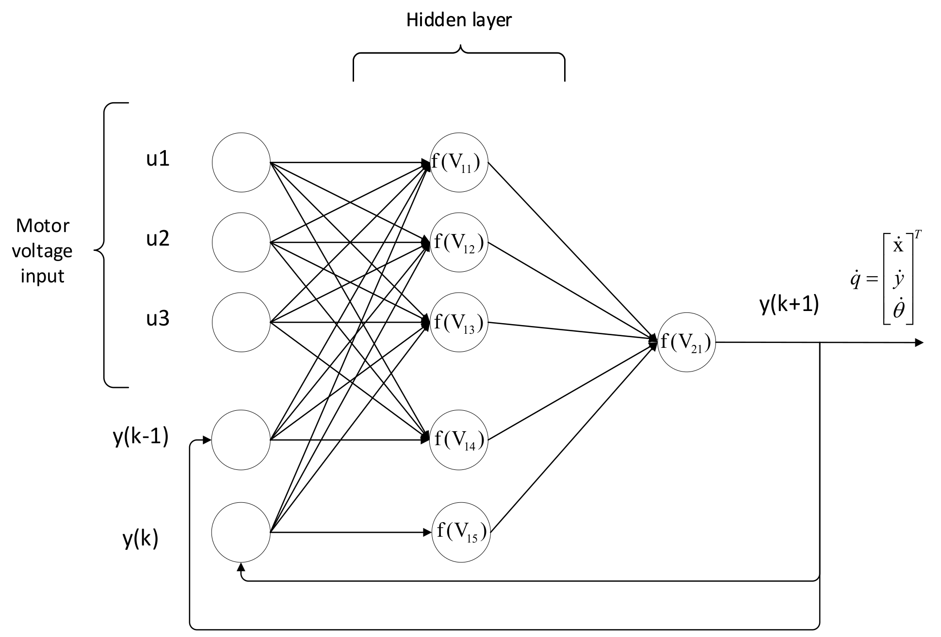
NARX neural network is a typical dynamic recurrent neural network, which is generally composed of an input layer, a hidden layer, and an output layer. The output of NARX neural network not only depends on the current input, but also related to the output of the past moment. It can accommodate sufficient historical data and the characteristics of changes between data. Therefore, the NARX network model can better approximate nonlinear dynamics model.

The reason for choosing NARX neural network is that the network can feed back output results during the training process, so it contains long-term information of the sequence, has long-term memory capabilities, and can simulate the long-term dynamics of the time sequence. At the same time, in the network training process, the network needs to be expanded in time sequence, and the output delay provides a shorter path for the propagation of gradient information, reducing the sensitivity of the network to long-term time dependence, so the convergence performance and generalization ability are better. Figure 3 shows the NARX neural network model structure of the omnidirectional mobile robot.

Among them, the input of the network model are the voltage $u={\left[u_1{u}_2{u}_3\right]}^T$ of the three motors of the mobile robot, and the output are the speed vector $\dot{q}={\left[\dot{x}\dot{y}\dot{\theta }\right]}^T$ of the omnidirectional mobile robot in the global coordinate system. The time delay of the neural network is 2, using a single hidden layer, each hidden layer includes five neurons, and the activation function use the Sigmoid function.

3.2. NARX Neural Network Training Data Selection And Experiment

NARX neural network’s training data uses the data measured by the omnidirectional mobile robot running at different moving speeds and different rotation angular speeds. The set moving speeds are 0.3 m/s, 0.5 m/s, 0.7 m/s, 1 m/s, 1.5 m/s, the set rotation speeds are 1 rad/s, 1.5 rad/s, 2 rad/s, 2.5 rad/s, 3 rad/s, record the required relevant data during 25 experiments, and each kind of moving speed will go ahead along the set 2 m × 2 m square trajectory at different rotational angular speeds. Among them, the three motor voltages of the mobile robot are the input data of the NARX neural network, and the $X,Y$-axis movement speed and rotation angular velocity which calculated by the sensor measurement are used as the expected output data of the NARX neural network. Use the Levenberg-Marquardt method to train NARX neural network. The output of the trained neural network model is as follows:

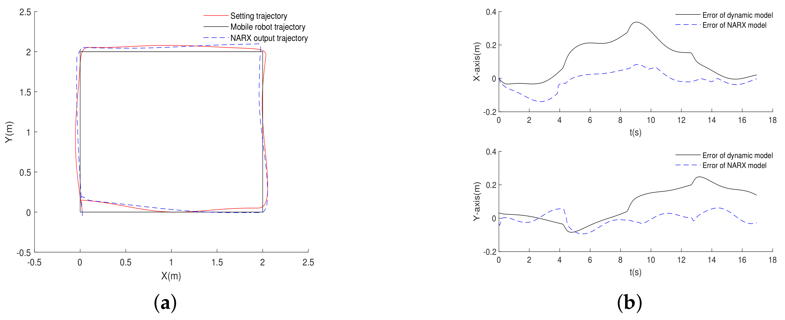
Figure 4 shows the output of NARX neural network model and error comparison. It can be seen that the NARX neural network output after data training is basically consistent with the trajectory output of the mobile robot. The curves in Figure 4b are the errors of the mobile robot trajectory with dynamics model and NARX neural network model in $X,Y$-axis directions respectively. It shows that the neural network can effectively replace the dynamic model with a very small error when the mobile robot rotating with moving. However, it is not enough to match the actual output numerically. The following will introduce a method to analyze the stability of the NARX neural network.

4. NARX Neural Network Stability Conditions

Before analyze stability of the trained NARX neural network, it is necessary to linearize it and transform it into a set of state space matrices. Then, a novel APLF method is used to analyze the stability of the neural network model in zero input state.

4.1. Use LDI Method to Represent NARX Neural Network

In this section, the method of using Linear Differential Inclusions (LDI) represent the trained NARX neural network we will be introduced [16].

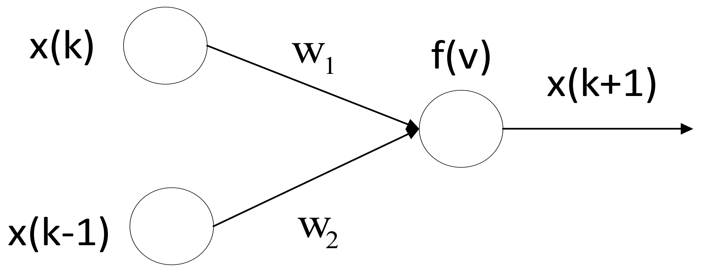
The single neuron structure in Figure 5 can be described by the following formula:

$$v=w_{1}x\left(k\right)+w_{2}x(k-1)$$

(19)

$$x(k+1)=f\left(v\right)$$

(20)

where $w_1$ and $w_2$ are the connection weight values, and $f\left(v\right)$ is the Sigmod activation function and is defined as:

$$f\left(v\right)=\left(\frac{2}{1+exp(-v/q)}-1\right)$$

Parameter q is the $f\left(v\right)$ correlation coefficient and greater than zero. In addition, $f\left(v\right)$ and its derivative satisfy the following constraints:

$$g_{1}v\le f\left(v\right)\le g_{2}v,\mathrm{v}\ge 0g_{2}v\le f\left(v\right)\le g_{1}v,\mathrm{v}\le 0$$

$${\mathrm{g}}_1=\underset{v}{min}{f}^{\prime }\left(v\right)=0,{\mathrm{g}}_2=\underset{v}{max}{f}^{\prime }\left(v\right)=0.5/q$$

where $g_1,g_2$ are the minimum and maximum values of $f^{\prime }\left(v\right)$ respectively. Furthermore, Equations (19) and (20) can be written as follows:

$$\begin{array}{c}x(k+1)=f\left(v\right)=(h_1\left(k\right)g_1+h_2\left(k\right)g_2)v\\ ={\displaystyle \sum _{i=1}^2}{h}_i\left(k\right)g_i(w_{1}x\left(k\right)+w_{2}x(k-1))\end{array}$$

(21)

Furthermore, let $\mathbf{x}\left(k\right)={\left[x\left(k\right)x(k-1)\right]}^T$ and (21) can be written as:

$$x(k+1)=\sum _{i=1}^2{h}_i\left(k\right){\mathbf{A}}_{\mathbf{i}}\mathbf{x}\left(k\right),h_i\left(k\right)\ge 0\sum _{\mathrm{i}=1}^2{h}_i\left(k\right)=1$$

(22)

From (22), it can be known that the state space matrix set of a single neuron are:

$$A_1=\left[\begin{array}{cc}{g}_1{w}_1& g_1{w}_2\\ 1& 0\end{array}\right],A_2=\left[\begin{array}{cc}{g}_2{w}_1& g_2{w}_2\\ 1& 0\end{array}\right]$$

(23)

Using this LDI method for the NARX neural network in Figure 3. The output neuron is defined as:

$$\begin{array}{cc}\hfill y(k+1)& =f\left(V_{21}\right)=(h_{211}\left(k\right)g_{211}+h_{212}\left(k\right)g_{212})V_{21}\hfill \\ \hfill & =\sum _{l=1}^2{h}_{21l}\left(k\right)g_{21l}{V}_{21}\hfill \end{array}$$

where

$$\begin{array}{cc}\hfill V_{21}& =w_{211}f\left(V_{11}\right)+w_{212}f\left(V_{12}\right)+w_{213}f\left(V_{13}\right)\hfill \\ \hfill & +w_{214}f\left(V_{14}\right)+w_{215}f\left(V_{115}\right)\hfill \end{array}$$

Then

$$\begin{array}{cc}{V}_{21}\hfill & =w_{211}(h_{111}\left(k\right)g_{111}+h_{112}\left(k\right)g_{112})V_{11}+w_{212}(h_{121}\left(k\right)g_{121}+h_{122}\left(k\right)g_{122})V_{12}\hfill \\ \hfill & +w_{213}(h_{131}\left(k\right)g_{131}+h_{132}\left(k\right)g_{132})V_{13}+w_{214}(h_{141}\left(k\right)g_{141}+h_{142}\left(k\right)g_{142})V_{14}\hfill \\ \hfill & +w_{215}(h_{151}\left(k\right)g_{151}+h_{152}\left(k\right)g_{152})V_{15}\hfill \end{array}$$

(24)

By substituting (19) into (24)

$$\begin{array}{cc}{V}_{21}\hfill & ={\sum }_{v=1}^2{\sum }_{b=1}^2{\sum }_{m=1}^2{\sum }_{n=1}^2{\sum }_{z=1}^2{h}_{11v}\left(k\right)h_{12b}\left(k\right)h_{13m}\left(k\right)h_{14n}\left(k\right)h_{15z}\left(k\right)·\hfill \\ \hfill & \{w_{211}{g}_{11v}(w_{111}x\left(k\right)+w_{121}x(k-1))+w_{212}{g}_{12b}(w_{112}x\left(k\right)+w_{122}x(k-1))\hfill \\ \hfill & +w_{213}{g}_{13m}(w_{113}x\left(k\right)+w_{123}x(k-1))+w_{214}{g}_{14n}(w_{114}x\left(k\right)+w_{124}x(k-1))\hfill \\ \hfill & +w_{215}{g}_{15z}(w_{115}x\left(k\right)+w_{125}x(k-1))\}\hfill \\ \hfill & ={\sum }_{v=1}^2{\sum }_{b=1}^2{\sum }_{m=1}^2{\sum }_{n=1}^2{\sum }_{z=1}^2{h}_{11v}\left(k\right)h_{12b}\left(k\right)h_{13m}\left(k\right)h_{14n}\left(k\right)h_{15z}\left(k\right)·\hfill \\ \hfill & \{(w_{211}{g}_{11v}{w}_{111}+w_{212}{g}_{12b}{w}_{112}+w_{213}{g}_{13m}{w}_{113}+w_{214}{g}_{14n}{w}_{114}+w_{215}{g}_{15z}{w}_{115})x\left(k\right)\hfill \\ \hfill & +(w_{211}{g}_{11v}{w}_{121}+w_{212}{g}_{12b}{w}_{122}+w_{213}{g}_{13m}{w}_{123}+w_{214}{g}_{14n}{w}_{124}+w_{215}{g}_{15z}{w}_{125})x(k-1)\}\hfill \end{array}$$

(25)

The matrix representation can be obtained as

$$\begin{array}{c}y(k+1)=\sum _{l=1}^2\sum _{v=1}^2\sum _{b=1}^2\sum _{m=1}^2\sum _{n=1}^2\sum _{z=1}^2{h}_{21l}\left(k\right)h_{11v}\left(k\right)h_{12b}\left(k\right)h_{13m}\left(k\right)h_{14n}\left(k\right)h_{15z}\left(k\right)·\\ \left\{g_{21l}(w_{211}{g}_{11v}{w}_{111}+w_{212}{g}_{12b}{w}_{112}+w_{213}{g}_{12m}{w}_{113}+w_{213}{g}_{14n}{w}_{114}+w_{215}{g}_{15z}{w}_{115})x\left(k\right)\right.\\ \left.+g_{21l}(w_{211}{g}_{11v}{w}_{121}+w_{212}{g}_{12b}{w}_{122}+w_{213}{g}_{12m}{w}_{123}+w_{213}{g}_{14n}{w}_{124}+w_{215}{g}_{15z}{w}_{125})x(k-1)\right\}\end{array}$$

Then the state space matrix set of NARX neural network are:

$$A_{lvbmnz}=\left[\begin{array}{cc}{a}_1& a_2\\ 1& 0\end{array}\right]$$

(26)

where

$$\begin{array}{c}{a}_1=g_{21l}(w_{211}{g}_{11v}{w}_{111}+w_{212}{g}_{12b}{w}_{112}+w_{213}{g}_{12m}{w}_{113}+w_{213}{g}_{14n}{w}_{114}+w_{215}{g}_{15z}{w}_{115})\hfill \\ a_2=g_{21l}(w_{211}{g}_{11v}{w}_{121}+w_{212}{g}_{12b}{w}_{122}+w_{213}{g}_{12m}{w}_{123}+w_{213}{g}_{14n}{w}_{124}+w_{215}{g}_{15z}{w}_{125})\hfill \end{array}$$

4.2. Minimum Representation

From (26), it can be seen that the number of matrices obtained after linearization of the neural network is too large. At the same time, the number of LMIs are also large too, which is very unfavorable for calculation.The Parameter Region (PR) method is used below to find the state space matrix set The smallest representation in. The definition of minimum substitution is as follows:

Definition 1. 

A nonlinear system described by LDI, which consists only of vertex points, is said to be a minimum representation.

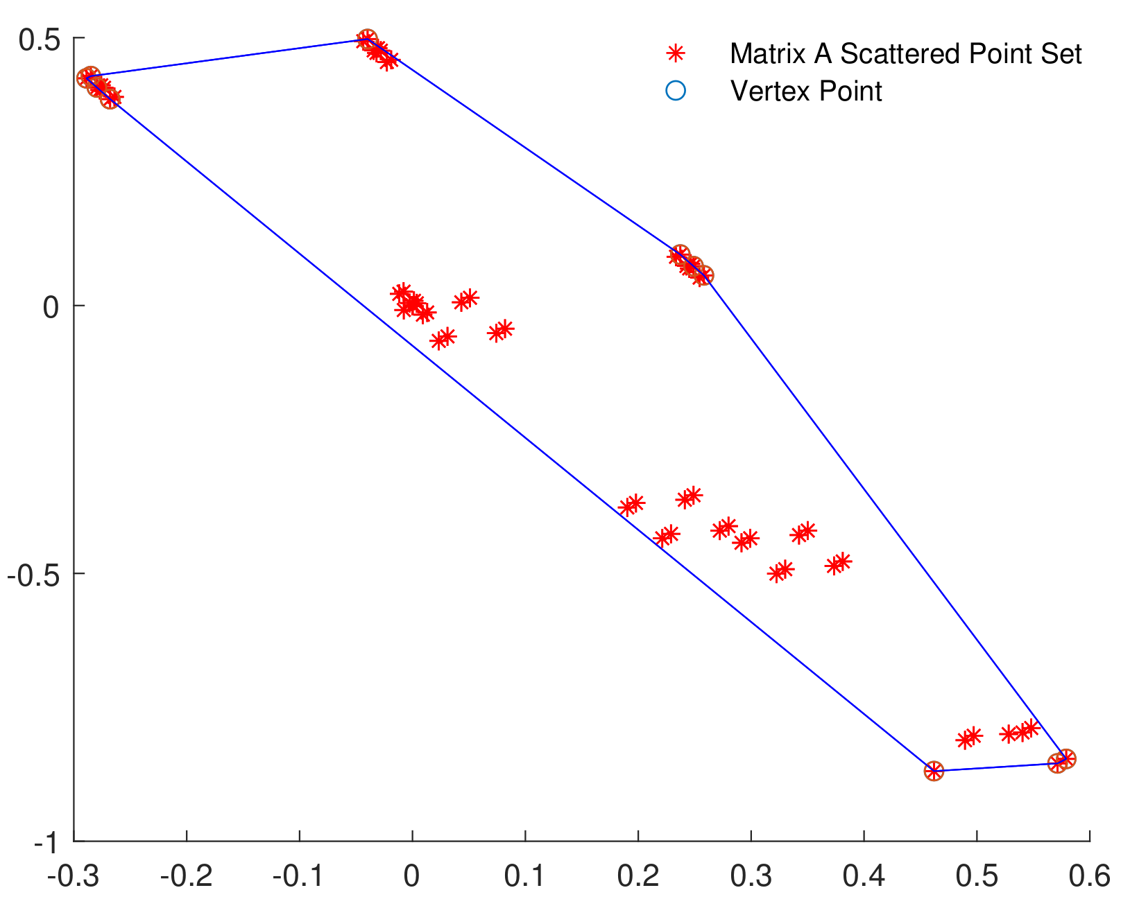
Equation $a_1$ and $a_2$ in (26) can be regarded as coordinate points in a two-dimensional coordinate system, and then the entire matrix set can be expressed as scatter points as shown in Figure 6:

The red star points in Figure 6 are the matrix A scatter point set. The polygon is used to enclose all coordinate points and the blue circle are its vertex points. The matrix A set represented by the blue circle are the minimum representation points of the LDI system. Furthermore, merge the vertices which are very close. Then, the final A matrix set are as follows:

$$\begin{array}{c}{A}_1=\left[\begin{array}{cc}-0.27& 0.41\\ 1& 0\end{array}\right]A_2=\left[\begin{array}{cc}-0.04& 0.52\\ 1& 0\end{array}\right]A_3=\left[\begin{array}{cc}0.25& 0.07\\ 1& 0\end{array}\right]\\ A_4=\left[\begin{array}{cc}0.57& -0.85\\ 1& 0\end{array}\right]A_5=\left[\begin{array}{cc}0.46& -0.87\\ 1& 0\end{array}\right]\end{array}$$

(27)

4.3. NARX Neural Network Stability Analysis

PDLF method is based on quadratic Lyapunov function and reduces the over conservatism of common Lyapunov function (CLF) [20,21,22]. In this chapter, in order to analyze the stability of NARX neural network system, the Activation Path-Dependent Lyapunov Function (APLF) method based on quadratic Lyapunov function is introduced. The $\xi \left(k\right)$ in PDLF only depends on the current step k. In APLF, however, $\xi \left(k\right)$ depends on the activation path value of $\xi \left(s\right)$, where $s\in [\mathcal{L},k]$, $\mathcal{L}<k$, and define $\mathcal{I}[k_1,k_2]\triangleq \{k_1,k_1+1,\dots ,k_2\}$.

During the each step interval $[k1,k2]$,using $h_j(k_2,k_1)$, $j\in \mathcal{I}[1,N^{k_2-k_1}]$ records the information of evolution of activation path-dependent value $\xi \left(k\right)$. Respect that

$$\begin{array}{cc}\hfill \sum _{j=1}^{N^{k_2-k_1}}{h}_j(k_2,k_1)& =\sum _{j=1}^{N^{k_2-k_1}}\left(\prod _{k=k_1}^{k_2-1}{\xi }_{i_k}\left(k\right)\right)=\prod _{k=k_1}^{k_2-1}\left(\sum _{i=1}^N{\xi }_i\left(k\right)\right)=1\hfill \\ \hfill h_j(k_2,k_1)& \ge 0,\forall j\in \mathcal{I}[1,N^{K_2-K_1}]\hfill \end{array}$$

(28)

Then, all system matrices $A_i,i\in \mathcal{I}[1,N]$ are recorded by the matrices $\mathcal{A}(k_2-k_1)$ during $[k_1,k_2]$. That is

$$\begin{array}{c}\hfill \mathcal{A}(k_2-k_1)=\prod _{k=k_1}^{k_2-1}{A}_{i_k},i_k\in \mathcal{I}[1,N]\end{array}$$

(29)

For the sake of simplicity for notations, define $k_{n+1}=k_n+K,n\in \mathbb{N}$, we denote $h\left(n\right)\triangleq h(k_{n+1},k_n),{\mathcal{A}}_j\triangleq {\mathcal{A}}_j(k_{n+1}-k_n)={\mathcal{A}}_j\left(k\right)$ and state transition matrix $\mathsf{\Phi }(n+1,n)$ can be expressed as

$$\begin{array}{cc}\mathsf{\Phi }(k_{n+1},k_n)\hfill & =\mathsf{\Phi }(n+1,n)={\prod }_{k=n}^{n-1}A\left(\xi \left(k\right)\right)\hfill \\ \hfill & ={\prod }_{k=n}^{n-1}\left({\sum }_{i=1}^N\xi \left(k\right)A_i\right)={\sum }_{j=1}^{N^K}{h}_j\left(n\right)\mathcal{A}\left(K\right)\hfill \\ \hfill & =\mathcal{A}\left(\theta \right(n\left)\right)\hfill \end{array}$$

(30)

where

$$\begin{array}{c}\mathcal{A}\left(h\left(n\right)\right)\in \{\mathcal{A}\left(h\left(n\right)\right):\mathcal{A}\left(h\left(n\right)\right)={\sum }_{j=1}^{N^K}{h}_j\left(n\right){\mathcal{A}}_j\}\hfill \\ {\mathcal{A}}_j={\prod }_{k=1}^k{A}_{i_k},i_k\in \mathcal{I}[1,N^K],j\in \mathcal{I}[1,N^K]\hfill \end{array}$$

(31)

Using $\xi \left(k\right)$ instead of $z\left(k\right)$ and the activation path-dependent vector is that

$$\begin{array}{c}\hfill h\left(n\right)={[h_1\left(n\right),\dots ,h_{N^K}\left(n\right)]}^T\in \mathit{H}\triangleq \{h\left(n\right):\sum _{i=1}^{N^K}{h}_j\left(n\right)=1,h_j\left(n\right)\ge 0\}\end{array}$$

(32)

In summary, the activation path-dependent parameter $h\left(n\right)$ of the NARX neural network system and system matrices ${\mathcal{A}}_j$ co-constructed a novel Activation Path-Dependent Lyapunov Function (APLF). That is

$$\begin{array}{cc}V\left(x\right(n),h(n\left)\right)\hfill & =x^T\left(n\right)P\left(h\left(n\right)\right)x\left(n\right)\hfill \\ P\left(h\right(n\left)\right)\hfill & ={\sum }_{j=1}^{N^K}{h}_j\left(n\right)P_j,P_j\ge 0,\forall j\in \mathcal{I}[1,N^K]\hfill \end{array}$$

(33)

The inequality is

$$\mathcal{A}{}_i^T{P}_j{\mathcal{A}}_{\mathrm{i}}-P_i\prec 0,\forall i,j\in [1,N^K]$$

(34)

The uncertain values $h\left(n\right)$ are represented by activation function, so could called it Activation Dependent. In addition, at step interval $[k1,k2]$ not only includes current uncertain values, but also involves past uncertain information and in a neural network system those uncertain values constitute lots of nodes during $[k1,k2]$, which connect with each other like a Path. That is the reason why the method in this paper is called in Activation Path-Dependent Lyapunov Function.

In method CLF, it chooses $P\left(\xi \right(k\left)\right)=P$, and, PDLF defines $P\left(\xi \left(k\right)\right)={\sum }_{i=1}^N{\xi }_i\left(k\right)P_i,\forall i\in \mathcal{I}[1,N]$, which makes PDLF more conservative than CLF. However, CLF and PDLF only include curent uncertain values, APLF contain uncertain values of past, that why CLF and PDLF are a special case of APLF.

In Equation (34) K is the step interval coefficient and determine the past uncertain values window. When K is large enough, the conservativeness of the APLF algorithm will approach to 0. Furthermore, N is the number of matrices, here set $N=5$. When $K=1$, substituting the A matrix set (27) into the inequality (34), the following P matrices is calculated to satisfy the corresponding LMI problems:

$$\begin{array}{c}{P}_1=\left[\begin{array}{cc}2.64& -0.49\\ -0.49& 1.34\end{array}\right]P_2=\left[\begin{array}{cc}2.36& -0.38\\ -0.38& 1.46\end{array}\right]P_3=\left[\begin{array}{cc}2.27& -0.18\\ -0.18& 1.13\end{array}\right]\\ P_4=\left[\begin{array}{cc}2.53& -0.72\\ -0.72& 2.01\end{array}\right]P_5=\left[\begin{array}{cc}2.39& -0.59\\ -0.59& 2.03\end{array}\right]{\mathrm{P}}_{\mathrm{i}},i\in \left[1,{\mathrm{N}}^{\mathrm{K}}\right]\end{array}$$

When $K=2$ and $K=3$, there are corresponding P matrices that satisfies the inequality equation in Formula (34), and the corresponding P matrices is not listed due to space limitations. Because of the existence of the P matrices, the NARX neural network represented by LDI is stable, so the dynamic model of the mobile robot identified by NARX is consistent in nature with the real mobile robot. Current APLF method needs to calculate all LMIs to analyze the stability of the system. For reducing the number of LMIs and calculation time, an optimized APLF method will be introduced next.

5. Optimized APLF Method

The basic drawback of APLF method is that the number of LMI increases exponentially with the increase of K. This chapter will introduce the optimized APLF method, It costs a lot of computation to analyze the subset of vertex or scheduling parameter trajectories [29].

Put matrix A (29) into Equation (33), set $K=3$, then ${\mathcal{A}}_n$ has the following situations

$$\begin{array}{c}\hfill {\mathcal{A}}_1=A_1·A_1·A_1,{\mathcal{A}}_2=A_1·A_1·A_2,{\mathcal{A}}_3=A_1·A_2·A_2{\mathcal{A}}_4=A_1·A_2·A_3\end{array}$$

(35)

The situations described in equation (35) are just a few cases in $N^K=125$. Using number records and set the collection to $\mathsf{\Theta }$:

$$\begin{array}{c}\hfill \mathsf{\Theta }=\left\{(1,1,1),(1,1,2),(1,2,2),(1,2,3)\right\}\end{array}$$

(36)

The sequence contained in $\mathsf{\Theta }$ is called a scenario sequence, and add a rate $\gamma$ into Equation (34):

$$\mathcal{A}{}_i^T{\mathrm{P}}_j{\mathcal{A}}_{\mathrm{i}}-{\gamma }^{2K_i}{P}_i⪯0,\forall i,j\in \mathsf{\Theta }$$

(37)

where $K_i$ is the length of the subsequence in $\mathsf{\Theta }$, when $\gamma <1$, it can be said that it is stable under discrete decay rate $\gamma$. It has been proved in the paper [29] that when $\gamma <1$ and there is a scenario sequence $\mathsf{\Theta }$ satisfying the formula (39), the system is asymptotically stable. The algorithm details are as follows:

Usually, set $\mathsf{\Theta }=\{1,2,3\}$. Define ${\gamma }_{\mathsf{\Theta }}^{*}$ is the minimum $\gamma$, ${\overline{\gamma }}_{min}=ma{x}_{\mathbf{i}\in \mathsf{\Theta }}max{\left(abs\left(eig\left({\mathcal{A}}_{\mathbf{i}}\right)\right)\right)}^{1/K_{\mathbf{i}}}$. Furthermore, $\sigma =ma{x}_{i\in \mathcal{I}}\overline{\sigma }\left({\mathcal{A}}_i\right)$, where $\overline{\sigma }$ denotes the maximum singular value, and ${\overline{\gamma }}_{sv}=ma{x}_{\mathbf{i}\in \mathsf{\Theta }}\overline{\sigma }{\left({\mathcal{A}}_{\mathbf{i}}\right)}^{1/K_{\mathbf{i}}}$. Then, ${\overline{\gamma }}_{min}\le {\gamma }^{*}\le {\gamma }_{\mathsf{\Theta }}^{*}\le {\overline{\gamma }}_{sv}\le \sigma$. If choose a longer sequence $\mathsf{\Theta }$, will get a smaller ${\gamma }^{*}$. However, the optimization algorithm will not work, when try all the sequence $\mathsf{\Theta }$. Next, use Algorithm 1 to calculate the data in example (27). The information of optimized APLF approach and its comparison with APLF approach is shown in

Table 2. Comparison between optimized APLF and original APLF.

Method	APLF			Optimized APLF
K	1	2	3	1	2	3	4
Computation time(s)	3.2	57.5	663	4.7	29.7	72.7	153.8
Number of LMI	30	650	15751	30	380	812	1406
Number of P ∖ Lenth of $\mathsf{\Theta }$	5	25	125	5	19	28	37
${\gamma }_{\mathsf{\Theta }}^{*}$	-	-	-	0.8516	0.8459	0.8418	0.8418

.

In Table 2, it can be see, As the memory value K grows. The optimized APLF method needs to calculate the number of LMIs and the time required to complete the calculation is significantly less than the APLF method. Case the optimized APLF only needs to calculate a specific sequence instead of all $N^K$ sequences.An interesting fact is that when $K=1$, the computation time of the original APLF is less than the optimized APLF method. Because it takes time to find the minimum $\gamma$, namely ${\gamma }_{\mathsf{\Theta }}^{*}$, in the optimized APLF method. However, when $K\ge 2$, the computation time required for the optimized APLF and the number of LMI are much less than the original APLF method.This means that after greatly reducing the computation time and the number of LMI calculations, the stability analysis of the neural network control system can be converted from offline analysis to online analysis, which expands the application scenarios and increases the practicability, such as self-driving cars, drones, etc. Moreover, ${\gamma }_{\mathsf{\Theta }}^{*}=0.8418<1$ ensures that the NARX neural network system is stable and can be expressed as the dynamic model of omnidirectional mobile robot.

Algorithm 1 optimized APLF

Set ${\mathsf{\Theta }}_{\left[1\right]}=\{1,2,3\},n=1,\underline{\gamma }=0,\tilde{\gamma }=+\infty$. Compute ${\gamma }_{{\mathsf{\Theta }}_{\left[n\right]}}^{*}$, by minimising $\gamma$ in Equation (37). Compute lower bound ${\overline{\gamma }}_{min}$ for scenario ${\mathsf{\Theta }}_{\left[n\right]}$. Let $\underline{\gamma }=max(\underline{\gamma },{\overline{\gamma }}_{min})$,$\tilde{\gamma }=min(\tilde{\gamma },{\gamma }_{{\mathsf{\Theta }}_{\left[n\right]}}^{*})$. if $\tilde{\gamma }-\underline{\gamma }<\epsilon (e.g.\epsilon =0.000001)$,END;we proved ${\gamma }^{*}\in [\underline{\gamma },\tilde{\gamma }]$. ELSE,find the sequences yielding active constraints: ${\mathbf{i}}^{\prime }=arg\underset{\mathbf{i}\in {\mathsf{\Theta }}_{\left[n\right]}}{max}\underset{\mathbf{j}\in {\mathsf{\Theta }}_{\left[n\right]}}{max}eig({\mathcal{A}}_{\mathbf{i}}^T{P}_{\mathbf{j}}{\mathcal{A}}_{\mathbf{i}}-{\gamma }_{\mathsf{\Theta }}^{*}{P}_{\mathbf{i}})$. Branch them either by incrementing its horizon one unit, or by appending every sequence of ${\mathsf{\Theta }}_{\left[n\right]}$; denote the resulting scenario as ${\mathsf{\Theta }}_{[n+1]}$.Let $n=n+1$. Go to step 2.

6. Conclusions

Based on the mechanical structure characteristics of the omnidirectional mobile robot, the force analysis has carried out to establish the dynamic model of the mobile robot. Because the dynamic model of mobile robot is complex, especially when it is rotating with moving, and there is a kinematic coupling situation. Therefore, the NARX neural network has been used to identify the dynamic model of the mobile robot. Furthermore, the qualitatively consistent between the NARX neural network and the dynamic model of mobile robot has been further verified, and the NARX neural network has been analyzed the stability. Firstly, the trained NARX neural network is represented by LDI and transformed into a set of several state space matrices A. Then, the PR method is used to find the minimum representation in the matrix set. Furthermore, APLF method is used to analyze the stability of NARX neural network. Finally, presents an optimized APLF method, which could reduce the number of LMIs and calculation time. The experimental results show that the dynamic model identified by NARX is consistent with the actual mobile robot.

References

- Asama, H.; Sato, M.; Kaetsu, H.; Ozaki, K.; Matsumoto, A.; Endo, I. Development of an Omni-Directional Mobile Robot with 3 DoF Decoupling Drive Mechanism. J. Robot. Soc. Jpn. 1996, 14, 249–254. [Google Scholar] [CrossRef]
- Salih, J.E.M.; Rizon, M.; Yaacob, S.; Adom, A.H.; Mamat, M.R. Designing Omni-Directional Mobile Robot with Mecanum Wheel. Am. J. Appl. Sci. 2006, 3, 1831–1835. [Google Scholar]
- Mamun, M.A.A.; Nasir, M.T.; Khayyat, A. Embedded System for Motion Control of an Omnidirectional Mobile Robot. IEEE Access 2018, 6, 6722–6739. [Google Scholar] [CrossRef]
- Rohrig, C.; Hess, D.; Kirsch, C.; Kunemund, F. Localization of an omnidirectional transport robot using IEEE 802.15.4a ranging and laser range finder. In Proceedings of the the 2010 IEEE/RSJ International Conference on Intelligent Robots and Systems, Taipei, Taiwan, 18–22 October 2010; pp. 3798–3803. [Google Scholar]
- Li, Y.; Dai, S.; Zhao, L.; Yan, X.; Shi, Y. Topological Design Methods for Mecanum Wheel Configurations of an Omnidirectional Mobile Robot. Symmetry 2019, 11, 1268. [Google Scholar] [CrossRef] [Green Version]
- Gu, D.; Hu, H. Receding horizon tracking control of wheeled mobile robots. IEEE Trans. Control Syst. Technol. 2006, 14, 743–749. [Google Scholar]
- Tang, J.; Watanabe, K.; Shiraishi, Y. Design and traveling experiment of an omnidirectional holonomic mobile robot. In Proceedings of the IEEE/RSJ International Conference on Intelligent Robots and Systems, Osaka, Japan, 4–8 November 1996; Volume 1, pp. 66–73. [Google Scholar]
- He, W.; Chen, Y.; Yin, Z. Adaptive neural network control of an uncertain robot with full-state constraints. IEEE Trans. Cybern. 2015, 46, 620–629. [Google Scholar] [CrossRef]
- Pin, F.G.; Killough, S.M. A new family of omnidirectional and holonomic wheeled platforms for mobile robots. IEEE Trans Robot. Autom. 1994, 10, 480–489. [Google Scholar] [CrossRef]
- Sira-Ramirez, H.; Lopez-Uribe, C.; Velasco-Villa, M. Linear Observer-Based Active Disturbance Rejection Control of the Omnidirectional Mobile Robot. Asian J. Control 2012, 15, 51–63. [Google Scholar]
- Ren, C.; Li, X.; Yang, X.; Ma, S. Extended State Observer based Sliding Mode Control of an Omnidirectional Mobile Robot with Friction Compensation. IEEE Trans. Ind. Electron. 2019, 66, 9480–9489. [Google Scholar] [CrossRef]
- Mekonnen, G.; Kumar, S.; Pathak, P.M. A new dynamic control model with stability analysis for omnidirectional mobile robot. In Proceedings of the 2015 Conference on Advances in Robotics, Goa, India, 2–4 July 2015; pp. 1–6. [Google Scholar]
- Piroddi, L.; Spinelli, W. An identification algorithm for polynomial NARX models based on simulation error minimization. Int. J. Control 2003, 76, 1767–1781. [Google Scholar] [CrossRef]
- Anh, H.P.H.; Ahn, K.K.; Il, Y.J. Dynamic model identification of 2-axes PAM robot arm using neural MIMO NARX model. In Proceedings of the the 2008 Second International Conference on Communications and Electronics, Hoi An City, Vietnam, 4–6 June 2008. [Google Scholar]
- Tijani, I.B.; Akmeliawati, R.; Legowo, A.; Budiyono, A. Nonlinear identification of a small scale unmanned helicopter using optimized NARX network with multiobjective differential evolution. Eng. Appl. Artif. Intell. 2014, 33, 99–115. [Google Scholar] [CrossRef]
- Tanaka, K. An approach to stability criteria of neural-network control systems. IEEE Trans. Neural Netw. 1996, 7, 629–642. [Google Scholar] [CrossRef] [PubMed]
- Ge, S.S.; Hang, C.C.; Zhang, T. Adaptive neural network control of nonlinear systems by state and output feedback. IEEE Trans. Syst. Man Cybern. Part B (Cybern.) 1999, 29, 818–828. [Google Scholar] [CrossRef] [PubMed] [Green Version]
- Schmidhuber, J. Deep learning in neural networks: An overview. Neural Netw. 2015, 61, 85–117. [Google Scholar] [CrossRef] [PubMed] [Green Version]
- Dorato, P.; Tempo, R.; Muscato, G. Bibliography on robust control. Automatica 1993, 29, 201–213. [Google Scholar] [CrossRef]
- Daafouz, J.; Bernussou, J. Parameter dependent Lyapunov functions for discrete time systems with time varying parametric uncertainties. Syst. Control Lett. 2001, 43, 355–359. [Google Scholar] [CrossRef]
- Chesi, G.; Garulli, A.; Tesi, A.; Vicino, A. Polynomially parameter-dependent Lyapunov functions for robust stability of polytopic systems: An LMI approach. IEEE Trans. Autom. Control 2005, 50, 365–370. [Google Scholar] [CrossRef]
- Geromel, J.C.; Colaneri, P. Robust stability of time varying polytopic systems. Syst. Control Lett. 2006, 55, 81–85. [Google Scholar] [CrossRef]
- He, Y.; Liu, G.; Rees, D. New delay-dependent stability criteria for neural networks with time-varying delay. IEEE Trans. Neural Netw. 2007, 18, 310–314. [Google Scholar] [CrossRef]
- Guerra, T.M.; Kruszewski, A.; Lauber, J. Discrete Tagaki-Sugeno models for control: Where are we? Annu. Rev. Control 2009, 33, 37–47. [Google Scholar] [CrossRef]
- Xiang, W.; Lopez, D.M.; Musau, P.; Johnson, T.T. Reachable set estimation and verification for neural network models of nonlinear dynamic systems. In Safe, Autonomous and Intelligent Vehicles; Springer: Berlin/Heidelberg, Germany, 2019; pp. 123–144. [Google Scholar]
- Kruszewski, A.; Wang, R.; Guerra, T.M. Nonquadratic Stabilization Conditions for a Class of Uncertain Nonlinear Discrete Time TS Fuzzy Models: A New Approach. IEEE Trans. Autom. Control 2008, 53, 606–611. [Google Scholar] [CrossRef]
- Tognetti, E.S.; Oliveira, R.C.L.F.; Peres, P.L.D. ℌ∞ and ℌ2 nonquadratic stabilisation of discrete-time Takagi-Sugeno systems based on multi-instant fuzzy Lyapunov functions. Int. J. Syst. Sci. 2015, 46, 76–87. [Google Scholar] [CrossRef]
- Xiang, W. Parameter-memorized Lyapunov functions for discrete-time systems with time-varying parametric uncertainties. Automatica 2018, 87, 450–454. [Google Scholar] [CrossRef]
- Sala, A. Stability analysis of LPV systems: Scenario approach. Automatica 2019, 104, 233–237. [Google Scholar] [CrossRef]
- Fu, H.; Xin, L.; Wang, B.; Wang, Y. Trajectory Tracking Use Linear Active Disturbance Control of the Omnidirectional Mobile Robot. In Proceedings of the the 2019 IEEE International Conference on Mechatronics and Automation (ICMA), Tianjin, China, 4–7 August 2019. [Google Scholar]
Figure 1.
Robot coordinate frame and physical comparison: (a) Robot coordinate frame. (b) physical comparison.
Figure 2.
Comparison of dynamic model trajectory and mobile robot trajectory.
Figure 3.
NARX neural network structure.
Figure 4.
Comparison of NARX neural network output and mobile robot trajectory: (a) trajectory comparison. (b) error comparison.
Figure 5.
Single neuron structure.
Figure 6.
Parameter region of NARX neural network.