Investigation of Snake Robot Locomotion Possibilities in a Pipe
by
 , , , , , and
Ivan Virgala
1,* ,
,
Michal Kelemen
1, 
Pavol Božek
2,
Zdenko Bobovský
3,
Martin Hagara
1,
Erik Prada
1 ,
,
Petr Oščádal
3 and
Martin Varga
1 1
Faculty of Mechanical Engineering, Technical University of Košice, 04200 Košice, Slovakia
2
Faculty of Material Science and Technology in Trnava, Slovak University of Technology in Bratislava, 917 24 Trnava, Slovakia
3
Faculty of Mechanical Engineering, VSB-Technical University of Ostrava, 708 00 Ostrava, Czech Republic
*
Author to whom correspondence should be addressed.
Symmetry 2020, 12(6), 939; https://doi.org/10.3390/sym12060939
Submission received: 13 March 2020
/
Revised: 6 May 2020
/
Accepted: 7 May 2020
/
Published: 3 June 2020
(This article belongs to the Special Issue Symmetry in Mechanical Engineering Ⅱ)
Abstract
:This paper analyzed the locomotion of a snake robot in narrow spaces such as a pipe or channel. We developed a unique experimental snake robot with one revolute and one linear joint on each module, with the ability to perform planar motion. The designed locomotion pattern was simulated in MATLAB R2015b and subsequently verified by the experimental snake robot. The locomotion of the developed snake robot was also experimentally analyzed on dry and viscous surfaces. The paper further describes the investigation of locomotion stability by three symmetrical curves used to anchor static modules between the walls of the pipe. The stability was experimentally analyzed by digital image correlation using a Q-450 Dantec Dynamics high-speed correlation system. The paper presents some input symmetrical elements of locomotion and describes their influence on the results of locomotion. The results of simulations and experiments show possibilities of snake robot locomotion in a pipe.
1. Introduction
Snake robots are a special kind of kinematically redundant mechanism that have been a focus of researchers for several decades. Their kinematic structure allows them to be very flexible and adaptive to rough terrain. Conventional robots based on a wheeled or tank-belted undercarriage are suitable for many applications, and they are simple from the perspective of control [1]. There are also many pipe mechanisms based on biological mechanisms [2]. However, there are many situations where they cannot be used, for instance in terrain with large height differences or very narrow spaces such as pipelines or channels. Climbing on rods or trees is another very uncomfortable environment for any kind of robot. Snake robots can potentially be used in underwater applications, military exploration, medical operations, searching for survivors after disasters, and many more scenarios. Because snake robots are kinematically redundant, they can also perform motion optimization tasks within their control [3].
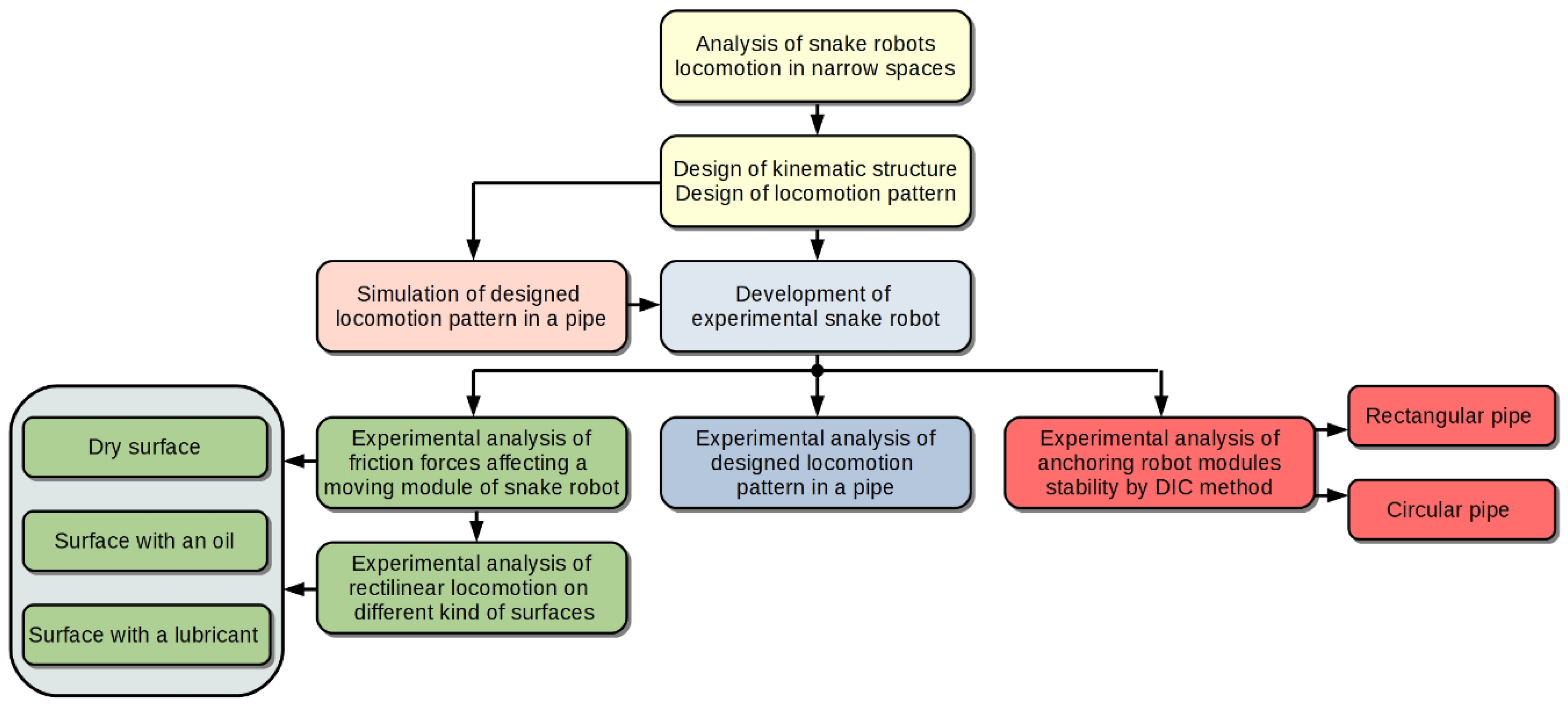
Our goal was to implement locomotion of an experimental snake robot in a pipe and investigate its possibilities while changing some of the input parameters. Our research was based on simulations as well as experiments, which can be divided into three areas. The block diagram of our research can be also seen in Figure 1. The paper is divided as follows: The second section introduces the current state of snake robots designed for locomotion in a pipe or channel. Next, the locomotion pattern is introduced and subsequently simulated in MATLAB R2015b. The designed pattern is also experimentally verified. Further experiments present the investigation of locomotion on dry, oily, and lubricated surfaces. The last part of the paper presents an experimental analysis of the possibilities of anchoring modules between the pipe walls by symmetrical curves. The analysis assumes a circular pipe as well as a rectangular cross-section. The conclusion discusses the possibilities for snake robot locomotion in a pipe.
2. Review of Snake Robot Applications in a Pipe
Research on snake robots started in the 1970s with the development of the first snake robot by Shigeo Hirose [4]. Since then, many experimental snake robots have been developed, with a focus on applications such as climbing, swimming, inspecting pipes, and moving through obstacles, among others. Although most previous works concentrated on a lateral undulation pattern of snake robots with or without active/passive wheels, few works dealt with pipe inspections.
Wakimoto et al. [5] presented the development of a micro robot that moves through pipes with different diameters using a traveling wave pattern. The maximum velocity of the robot was 36 mm/s and it was able to move in pipes with diameters from 18 mm up to 100 mm. Greenfield et al. described the locomotion pattern of a snake robot moving in a pipe [6]. They developed an algorithm for climbing, and the robot stabilized itself against gravity by pressing outward to induce friction. In 2006, Brunete et al. developed a micro snake robot with two degrees of freedom (DOF) per module [7]. The robot was able to perform locomotion in different pipes and elbows. In [8], Barazandeh proposed a mathematical model of a climbing snake robot using a concertina pattern. By optimizing the proposed model, the results showed that self-locking could occur during the course of climbing, resulting in zero actuator torque. The authors claimed that there should be a minimum number of contact points to activate self-locking in a climbing robot. This number depends on the weight of the robot modules and the friction coefficient. Wright et al. developed a modular snake robot consisting of 16 modules with a modified hobby servomotor [9]. This robot was able to climb inside and outside of a pipe. Another study [10] presented a snake robot with the ability to travel through pipes. The authors proposed three control algorithms: force control, and adjusting controls to changing pipe diameter and curved pipe. This team realized traveling in several kinds of pipelines by an experimental snake robot using 13 intelligent actuators. In [11], Andruska and Peterson demonstrated how to control a hyper-redundant snake robot in a compliant elastic environment such that it was able to navigate paths with unknown curvature radius. Akbarzadeh et al. [12] presented a novel kinematic modelling approach for snake robot motion with a concertina pattern. Their approach provides flexibility for natural locomotion. The paper also presented a dynamic curve whose shape can be easily modified by a single parameter. Their approach was verified by simulations in Webots. In 2012, Marvi and Hu performed a series of experiments to measure the friction of corn snakes while climbing through a channel [13]. They proposed a theoretical model to predict the snake’s traverse force. Their investigations showed that the snake moved in a channel by a series of extensions and contractions in which portions of its body extended forward while the rest was anchored. Other researchers [14] modelled snake locomotion on the basis of autonomous decentralized control. By simulations, they demonstrated that the locomotion pattern smoothly changed from sinus-lifting to concertina. Our research team also contributed to this area [15]. Our paper dealt with a snake robot moving in a pipe using a traveling wave pattern. Locomotion in straight and curved pipes was demonstrated by an experimental snake robot consisting of 11 DOF. An analysis of a snake robot moving by rectilinear motion in a pipe is presented in [16]. A novel gait based on cylinders as well as arboreal concertina locomotion for a snake robot was proposed in [17]. The authors also introduced a kinematic and dynamic analysis of gait, and the developed approach was verified by simulations in V-REP. Within the simulations, the snake robot climbed on a rod using the concertina principle. Studies on the low-cost application of a snake robot at a large-scale nuclear power facility to sense pipe components was presented in [18]. Within this study, the locomotion method was developed and executed in a narrow space. The developed algorithm was based on angular changes of various modules of the snake robot.
By summarizing previous works focused on snake robot applications in pipes or channels, we can say that the three main locomotion patterns are concertina, rectilinear, and traveling wave. Looking at the whole research area of snake robots, a small percentage of previous works were devoted to locomotion in confined spaces such as pipes or channels. We would like to contribute to this area with this study, including the design of a new locomotion pattern, simulations, the design of a new unique experimental snake robot, and an experimental analysis of locomotion.
3. Design and Analysis of Locomotion Pattern in a Pipe
Snake robots have great potential to be applied in various kinds of environments, such as narrow spaces, rough terrains, smooth surfaces, underwater, tall heights, and many more. In all these environments, a biological snake would perform different kinds of natural locomotion patterns. For example, to move underwater it could use a lateral undulation pattern, for heights it could use a climbing pattern, and in a pipe it could use a concertina pattern.
Our analysis deals with applications in narrow spaces. From previous studies on biological snakes, it is clear that snakes use concertina locomotion in narrow spaces [19]. Concertina locomotion consists of several phases. First, the snake pushes against the constrained environment with the rear part of its body. This activity we consider to be an anchoring of snake modules. Subsequently, the snake straightens its body along the direction of motion, while the rear part is anchored. The anchored part can be considered static. The next phase is based on pushing the front of the body against the constrained environment (the front part is now static, or anchored), while it pulls its rear parts to the front. By repeating these phases, the snake is able to achieve forward locomotion. In special cases of constrained environments such as very narrow spaces, a snake is also able to use rectilinear locomotion. During rectilinear locomotion, the rear parts of the body are static, while the front parts move forward by muscular activity. After this phase, by the weight of the static front parts, the rear parts can be drawn to the front along the direction of motion. A snake uses this kind of locomotion especially when it is in a very narrow space and is unable to perform a different kind of locomotion.
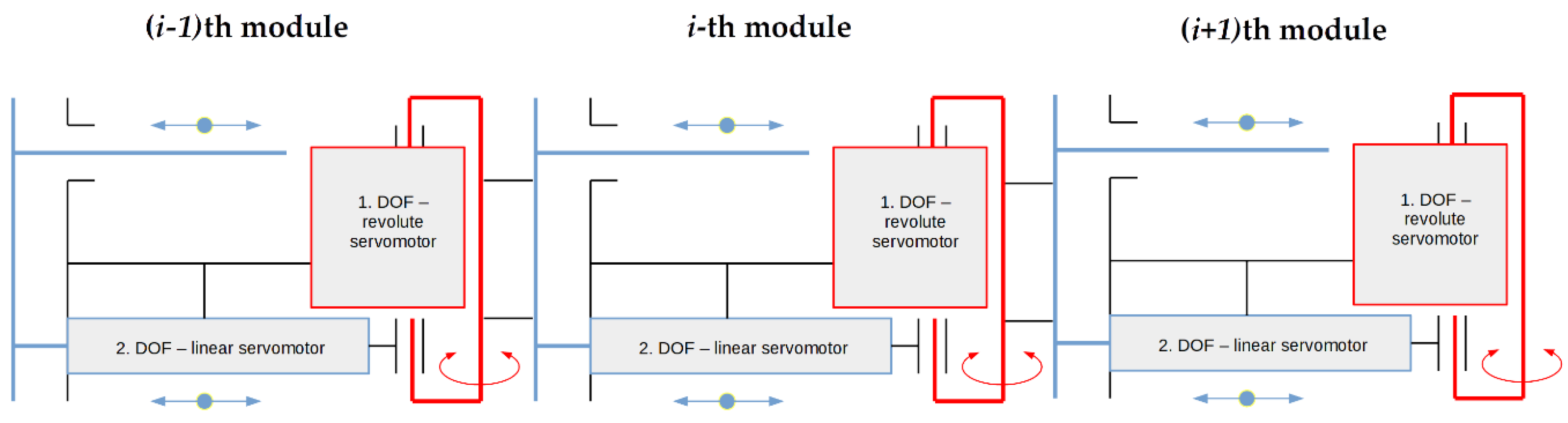
These two biological snake patterns, rectilinear and concertina, are the basis of this study. Let us consider a snake robot as a kinematically redundant mechanism consisting of many modules imitating a biological snake body. In order to analyze snake robot locomotion in narrow spaces, we consider a snake robot module having two DOFs: the first one considers revolute joints, the second considers linear joints. By connecting several modules together, each module is able to perform revolute and linear motion, according to the requirements of the desired application.
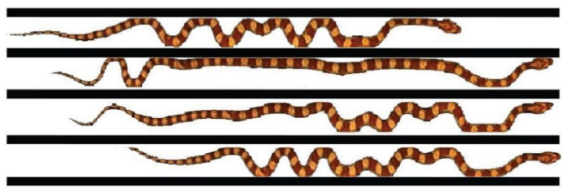
Figure 2 shows a video sequence of biological corn snake locomotion in a pipe [13]. The snake moves according to pattern described above.
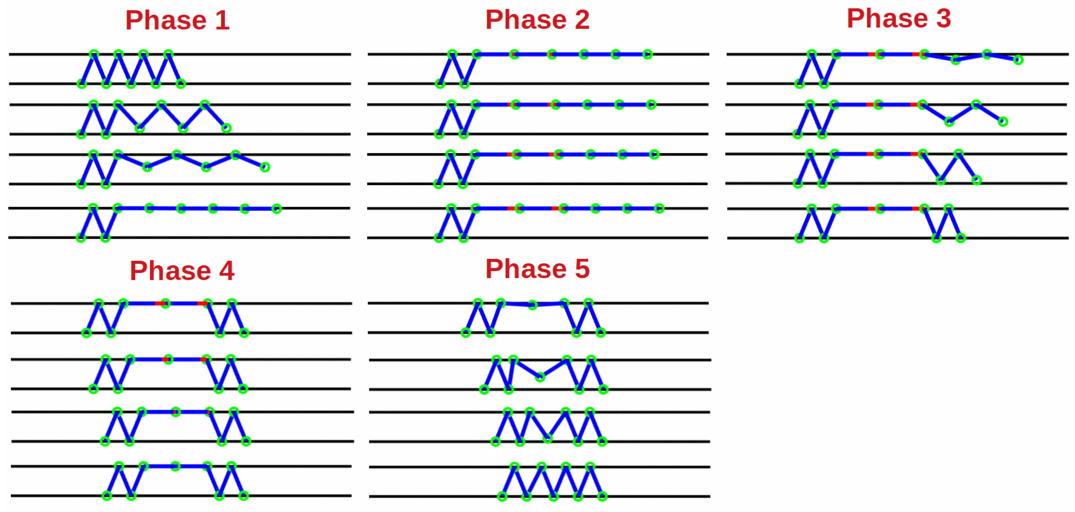
Referring to Figure 2, we designed a locomotion pattern for a snake robot with two DOFs per module. As can be seen from Figure 3, there was symmetrical behavior of the snake robot body. Except for the first and second phases, all other final states of individual phases were symmetrical, considering that the vertical axis of symmetry was in the middle joint of the snake robot.
Figure 3 assumes a triangular shape for the initial position of the locomotion cycle. The amplitude of the triangular shape is primarily formed by one robot module. However, if pipe diameter d (or for a theoretical, link-based robot) is greater than module length L, the amplitude of the triangular shape can be formed by two or more modules. By considering pipe diameter D, module length L, and maximal protrusion of linear joint l, the traveled distance of one locomotion cycle can be expressed as
Equation (1) considers exactly the pattern from Figure 3, so it means that the robot used three modules to anchor its body and two modules for linear motion. The pattern from Figure 3 can be also described by a general form:
where f is the number of anchoring modules, m is the number of snake robot modules, and n is the number of modules between the anchored rear and front modules; see the third phase in Figure 3. From Figure 3, d can be expressed as
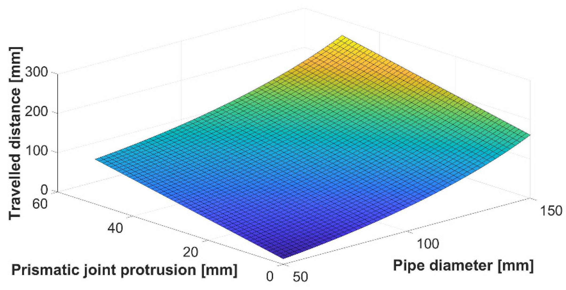
where represents the width of a snake robot module. Considering the link-based model, we can assume only parameter , but for a real snake robot it is necessary to consider the width of the module. The influence of pipe diameter D and linear joint protrusion l on traveled distance is expressed in Figure 4.
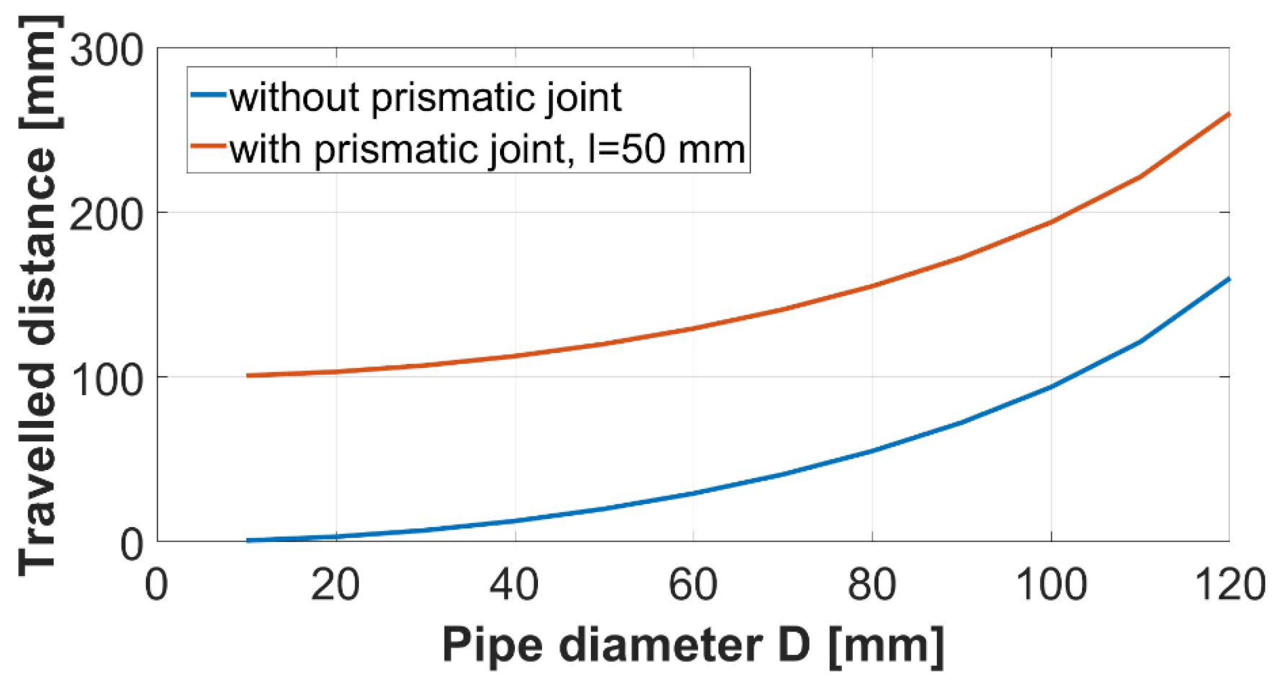
The real application of a snake robot, of course, considers the fixed value of module length L. Figure 5 shows how the traveled distance changes in relation to changes of the pipe diameter, while linear joint protrusion is neglected (shown in blue). The locomotion pattern described in Figure 3 can assume a version with or without linear joint protrusion. Assuming the protrusion is , the traveled distance of one locomotion cycle would be 100 mm more (see Figure 5 (shown in red)). By adding a linear joint to the module, the traveled distance per locomotion cycle significantly increases.
4. Simulation of Locomotion
This section presents a simulation of the introduced locomotion pattern. The aim of the simulation is to perform locomotion in a pipe, and also to verify it on the basis of the mathematical model from the previous section. The simulation parameters are as follows: the length of the snake robot module is , the maximum linear protrusion is , the maximum revolute joint motion is ±90°, and the number of snake robot modules is . The snake robot moves in a pipe with a rectangular cross-section with diameter .
The simulations were done in MATLAB R2015b. Joint angles were assembled in vector , where and is the number of locomotion phases, . We also defined vector as the vector of joint velocities for a particular locomotion phase and vector as the vector of joint accelerations for particular locomotion phase. Considering all phases of locomotion, the vector of joint angles is based on locomotion properties such as module length L and pipe diameter D. Vectors and are then determined on the basis of the fifth-order polynomial of particular joint angles , where , is the number of active phases of locomotion, and is the determined time for a particular phase. By using the fifth-order polynomial instead of the third-order polynomial, we can also control the acceleration of joints [20]. The third-order polynomial allows us only to control the position and velocity [21]. By derivation of we get , and subsequently by derivation of we get . On the basis of these terms and by substituting initial and final conditions of motion into these terms, we get the vector of coefficients . By computing vectors , , for all phases of locomotion , the locomotion of the snake robot for one cycle can be determined.
The graphical results of simulated snake robot locomotion in a pipe are shown in Figure 6.
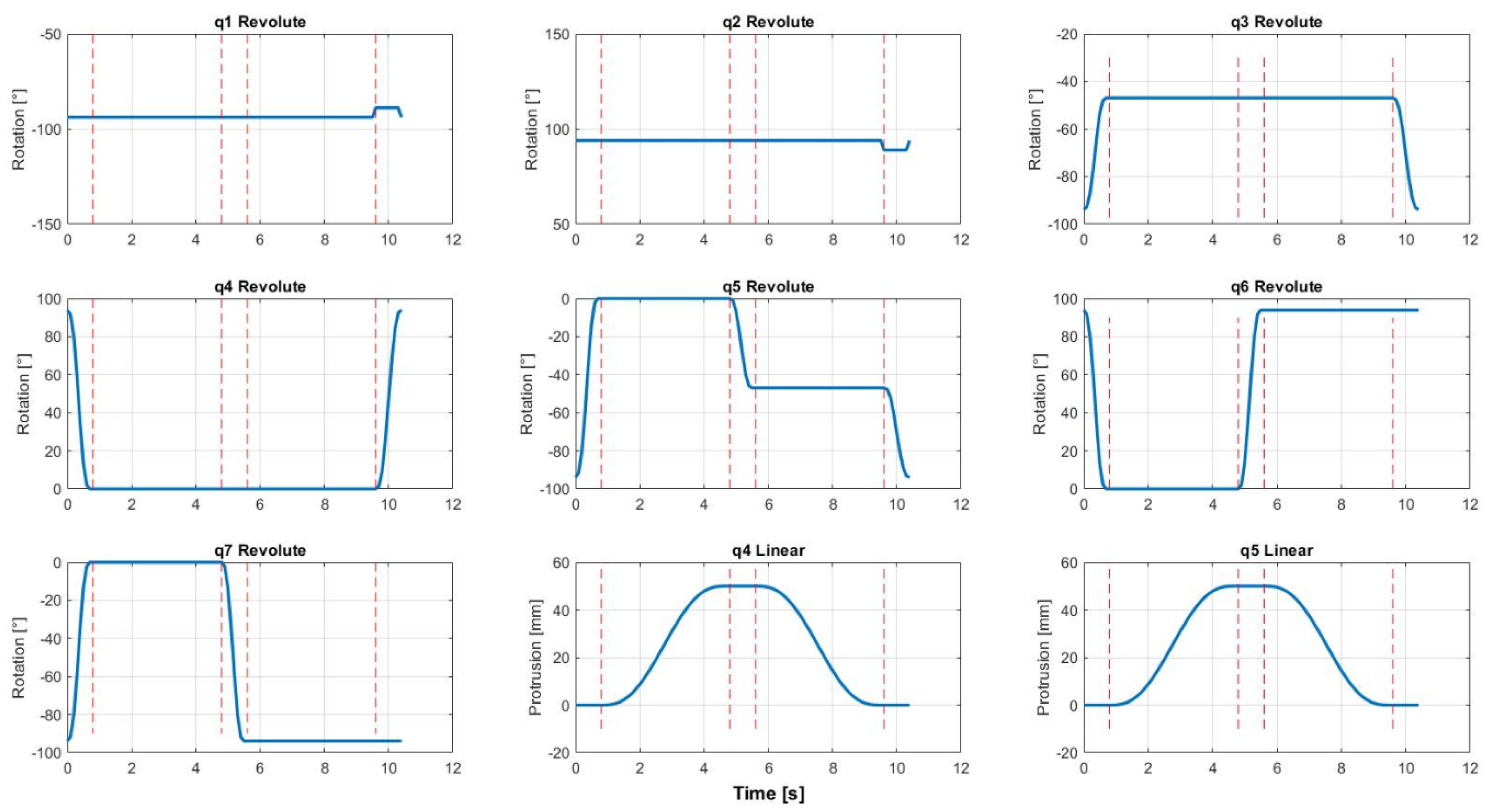
Figure 7 shows time courses of snake robot joints during concertina locomotion. The individual phases of locomotion are denoted by dotted red lines.
From the initial position of the snake robot, it extends most of its modules along the direction of motion. By pushing the last three modules against the walls of the pipe, the anchor effect occurs. Because of this anchor, the front modules are able to move forward without any backward motion. The linear motion of the two modules is shown in Figure 6 in red. They move as much as the range of linear actuators enables them. After this phase, the first three modules now serve as anchors in order to pull the rear modules to the front. It is clear that in this phase, the last three modules need to release the pressure against the walls of the pipe. Figure 6 represents only one locomotion cycle.
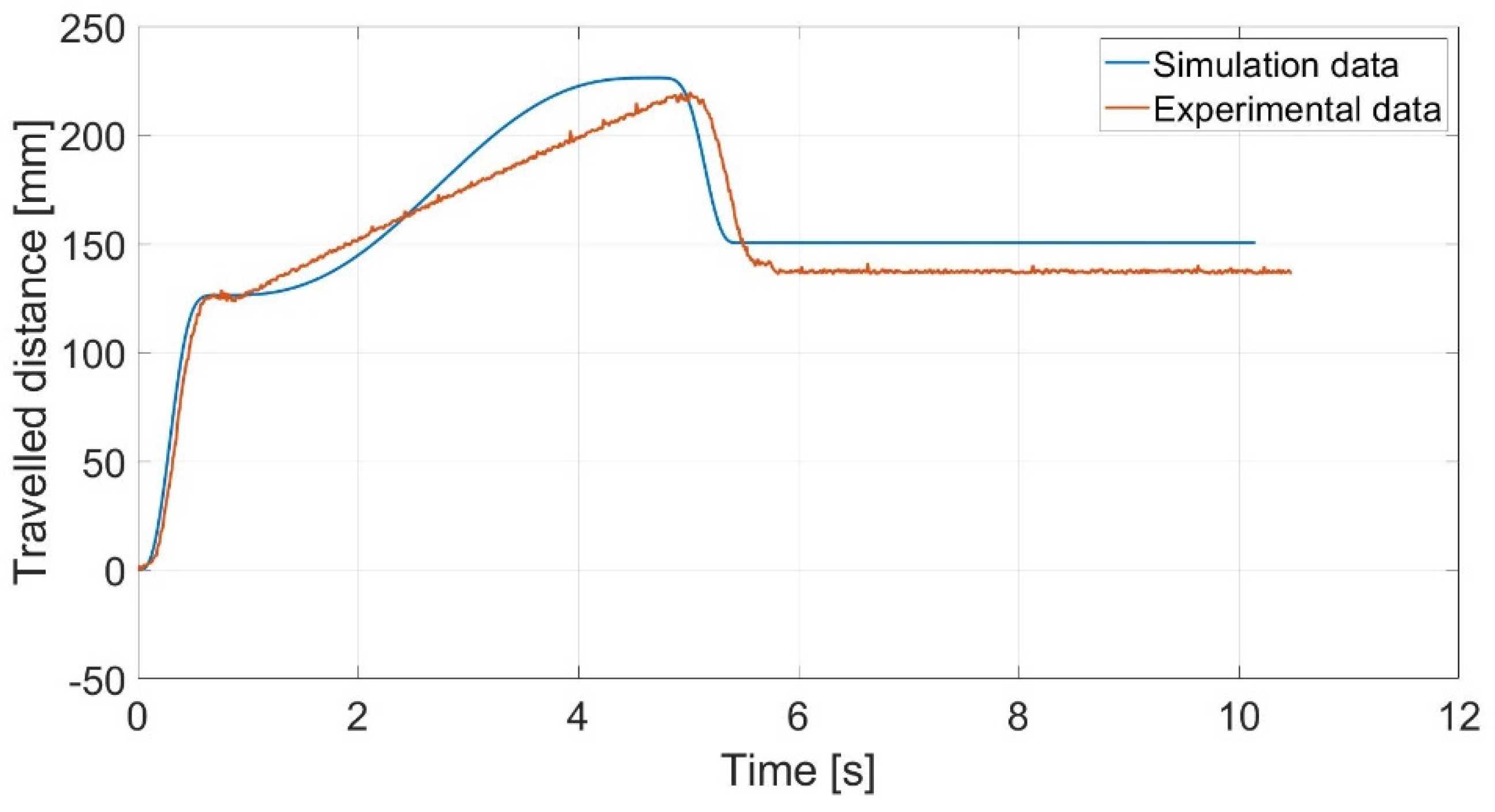
The vector of the head coordinates is represented by , where due to the planar task. Simulated coordinates of the head module during concertina locomotion are shown in Figure 14, along with experimental data.
5. Development of Experimental Snake Robot
This section deals with the experimental analysis of snake robot locomotion. Our team from Cognitics Lab at Technical University of Košice, Slovakia, developed a 14 DOF snake robot for experimental purposes.
5.1. Mechanical Design of Snake Robot
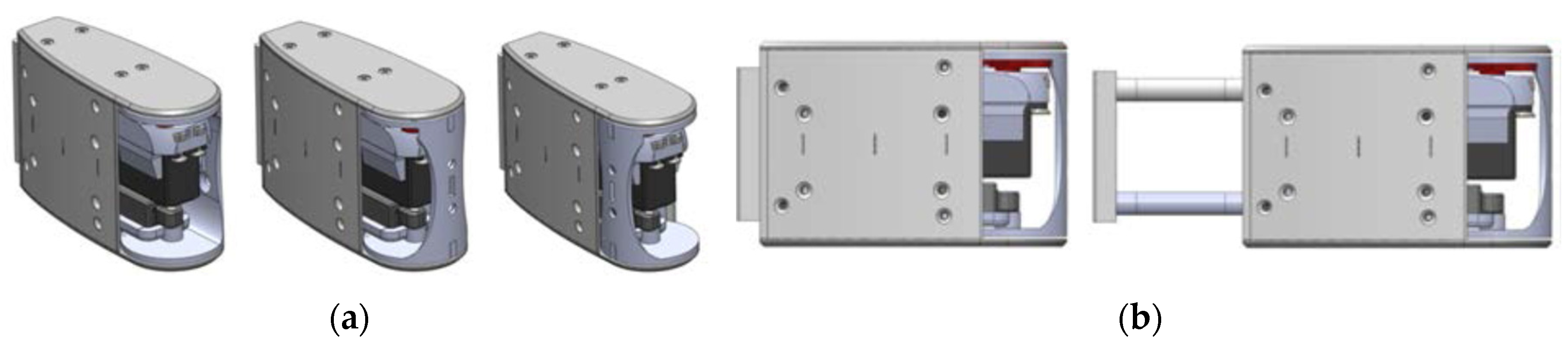
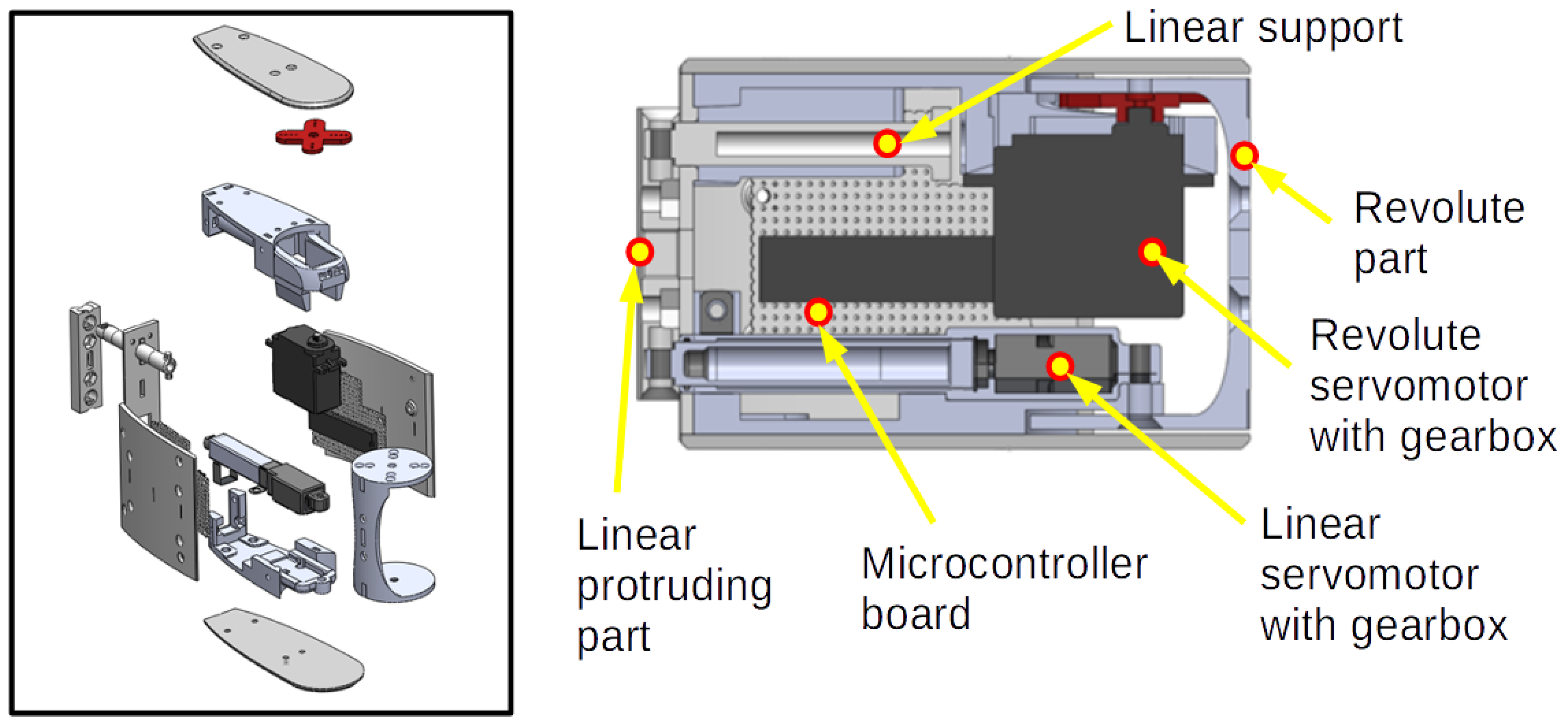
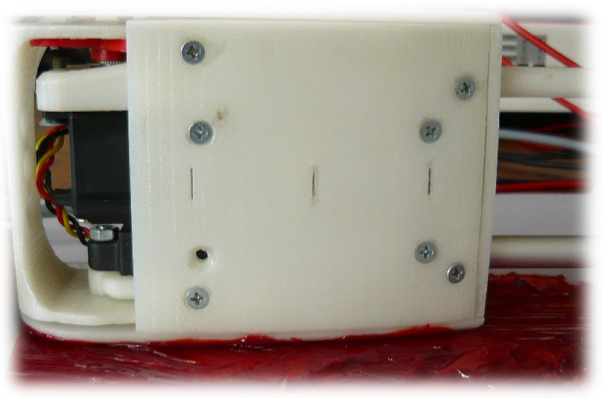
Our developed snake robot had a significant structure. Considering the joints of the robot module, while most experimental snake robots have one or two revolute joints per module, our robot had one revolute and one linear joint per module. The robot was designed for planar motion in pipes. Modules consisted of one revolute and one linear servomotor. The Hitec HS-645MG revolute servomotor has the following parameters: maximum catalogue torque 0.939 Nm (6 V DC), weight 55.2 g, and maximum speed 60°/sec (6V DC). For linear motion, a Firgelli L12 linear servomotor was used, with the following parameters: maximum force 42 N, maximum speed 13 mm/s, gear ratio 100:1, and weight 40 g. The range of revolute motion for each module was ±90° (see Figure 8a).
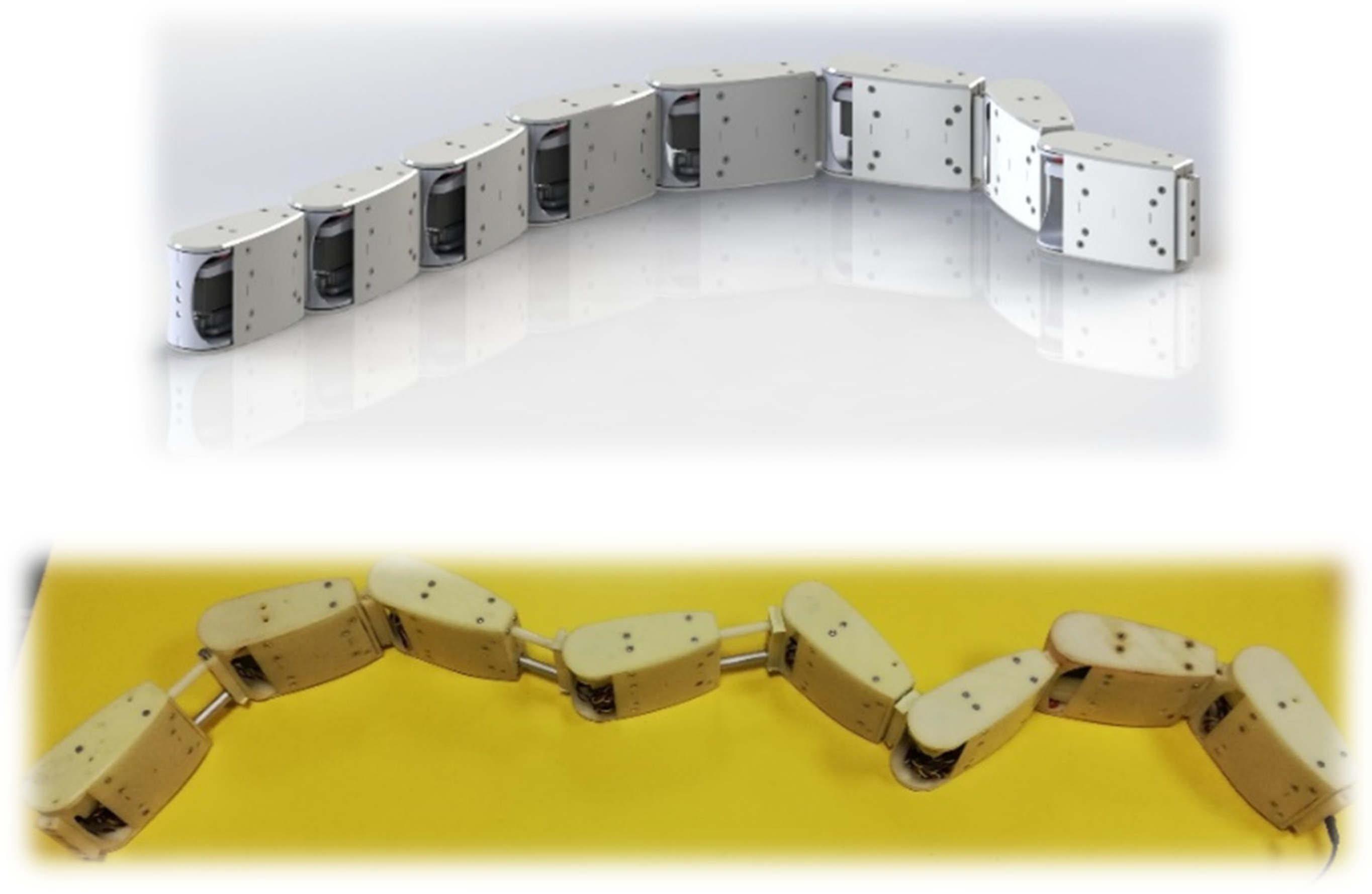
The range of linear motion for each module was 50 mm (see Figure 8b). The kinematic configuration of the robot module can be seen in Figure 9. The inside of the snake robot module is shown in Figure 10. The experimental snake robot consisted of eight identical modules, hence the whole robot had 14 DOF. Such kinematic redundancy represents great potential for the robot to be applied in narrow or geometrically complicated environments. The final model of the robot is shown in Figure 11. The top image in Figure 11 shows the final CAD model, and the bottom image shows the real snake robot.
All components for snake robot modules were printed by a 3D printer from ABS material. Each module weighed and had dimensions of 130 × 80 × 47 mm.
5.2. Electrical and Control System of Snake Robot
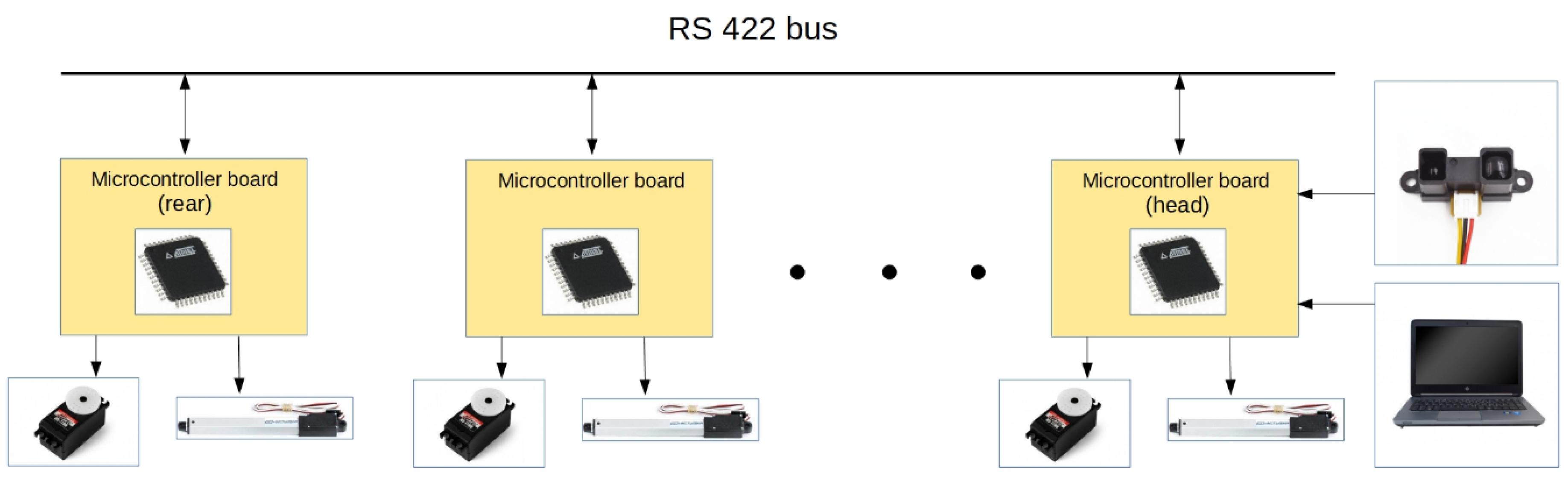
Each module of the snake robot had a separate circuit board based on an ATmega16 microcontroller working at frequency MHz. From Figure 12 it can be seen that the robot modules communicated with each other by RS422. The main control system ran in MATLAB R2015b, which communicated with the snake robot. Microcontrollers processed received signals with required revolution and linear position, and subsequently controlled the servomotor positions.
The snake robot had on its head module an optical distance sensor, with the opportunity to add a camera. The robot was supplied by external voltage.
6. Experiments with Snake Robot in a Pipe
This section describes three types of experiments. The purpose of the first experiment was to verify the designed pattern locomotion. The second experiment investigated the influence of different kinds of pipe surfaces on locomotion. The last experiment analyzed the anchoring of modules between pipe walls by means of three symmetrical curves applied to the anchored modules. The analysis was performed from the point of view of stability of the robot moving on an inclined surface during locomotion.
6.1. Locomotion Pattern in a Pipe
The first experiment tested the locomotion pattern introduced in previous sections. The snake robot was tested in a pipe with a rectangular cross-section with diameter . The length of each snake robot module was and the number of modules was . The robot used eight modules for locomotion, performing revolute as well as linear motion. The main control system ran in MATLAB R2015b.
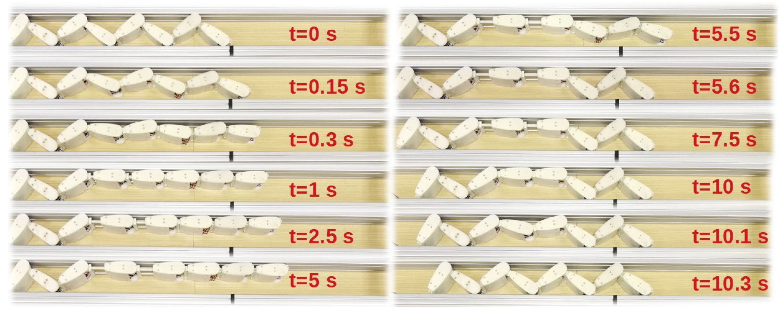
One locomotion cycle is shown in Figure 13. Considering the locomotion pattern introduced in Figure 3, Figure 13 shows the symmetrical behavior as well. The key point during a locomotion cycle was to ensure sufficient pressure between the anchored modules and the walls of the pipe. By comparing simulation and experimental results, we can see that real traveled distance was lower than theoretical traveled distance (see Figure 14). As can be seen from Figure 14, due to the linear motion of the servomotors, the robot performed a small backward motion (shown in red). The reason was imperfect anchoring of modules between the pipe walls. Other reasons for the variation in traveled distance were imprecise linear servo protrusion, idealizing of snake robot, and pipe dimensions, among others.
Because of the high gear ratio in the linear servomotor, the slowest part of locomotion was linear motion, which took around 4–5 s. In general, snake robots are not very fast; their superiority and excellence are in other properties. Nevertheless, the experiments showed the ability of a snake robot to perform locomotion in a narrow space. The proposed mathematical background also provided an approximate prediction of locomotion.
6.2. Locomotion on Different Surfaces
Let us consider a real application of a snake robot moving in a pipe. For a real application, we should also consider that the surface of the pipe would not be ideal. In a real application, the surface could be dirty and contain different kinds of sediment with dry or viscous properties, and the roughness of the surface could affect locomotion [22]. In many technical applications, high-precision motion control is required. However, their performance is limited by various nonlinear factors such as friction. For this reason, friction needs to be compensated many times [23].
The following section discusses basic friction models.
6.2.1. Friction Models
One of the basic friction models is called stiction. Stiction occurs in the case of zero mass velocity. The force required to overcome static friction is called breakaway force, which can be set according to Equation (4):
where is static friction force and is external force affecting the mass [24]. Once overcomes , the mass starts to move. From the point of view of numerical simulation, one of the main disadvantages of this friction model is its discontinuity at zero velocity of mass. This problem is usually overcome by some approximation, for example, by arctan function with suitable slope. On the other hand, the slope of arctan function can cause failure during numerical simulation due to very short integration time.
The next basic model is Coulomb friction mode. This model depends on mass velocity direction (not magnitude) . Considering the same materials of the surface, Coulomb friction coefficient is usually lower than static friction coefficient . Coulomb friction force, also known as kinetic friction, can be expressed by Equation (5) [25]:
where is a normal load between two contact surfaces. Function can be stated as
The next model, the so-called viscous friction model, occurs in the presence of oil. Oil or lubricant decreases the friction coefficient between two surfaces. The viscous friction model is described by Equation (7) [26]:
where is the viscous friction coefficient. This kind of model is different from the two previous models because of its linearity.
The last basic model is the Stribeck friction model. This model describes surfaces with the presence of liquid or solid oil. Stribeck friction can be expressed by Equation (8):
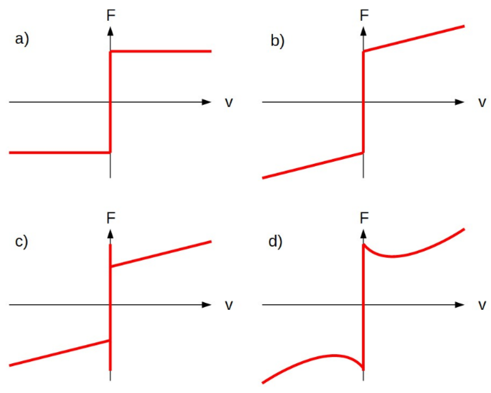
where is sliding speed, is Stribeck velocity, and k is an exponent. All mentioned friction models are shown in Figure 15.
6.2.2. Testing of Locomotion on Different Kinds of Surfaces
In this section, snake robot locomotion on three kinds of surfaces is investigated: a clean surface, and surfaces with oil and lubricant.
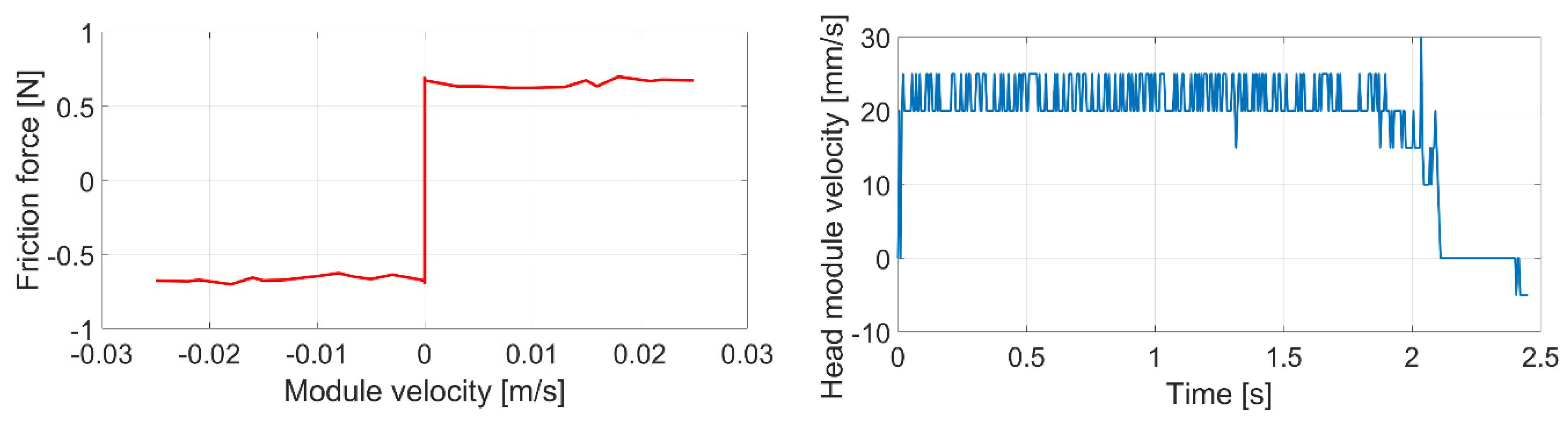
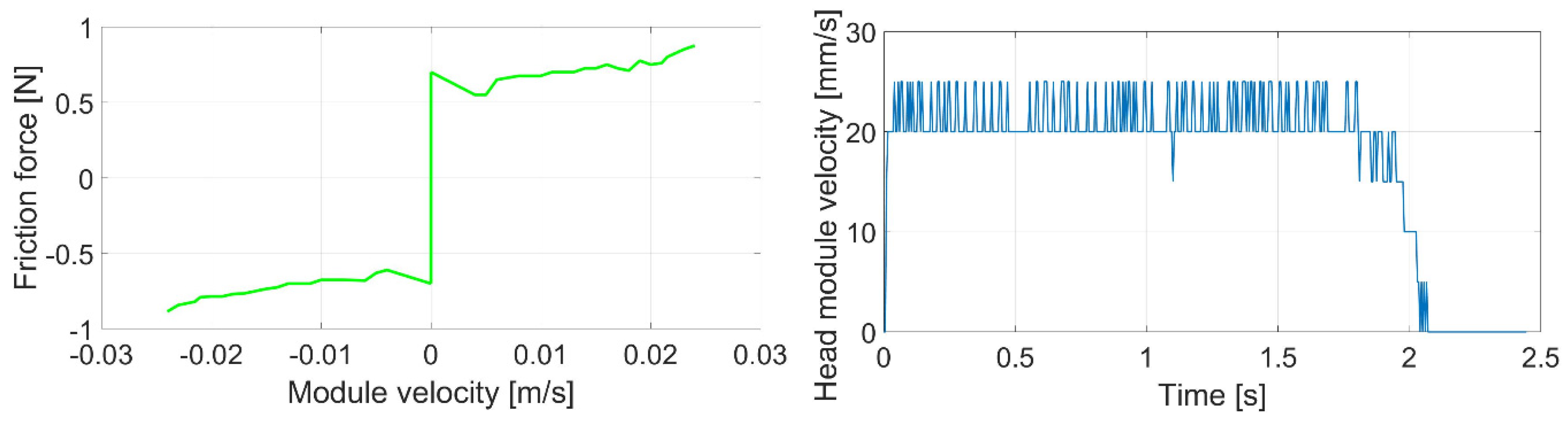
Only four snake robot modules were used for the experiment, following our previous analysis [16]. For measurements, we used a LARM MSL50 incremental linear sensor with measuring step of 5 μm. During the experiments, only the head module moved, while the other modules were static. The results of the first surface measurement are shown in Figure 16.
The graph on the left in Figure 16 represents measured friction force based on linear module velocity. The graph on the right represents a sample of a moving module by certain linear velocity. Considering these results and basic friction models shown in Figure 15, we can recognize a Coulomb friction model. Because the results in both directions of motion were almost the same, the final measured friction characteristic had a symmetrical pattern.
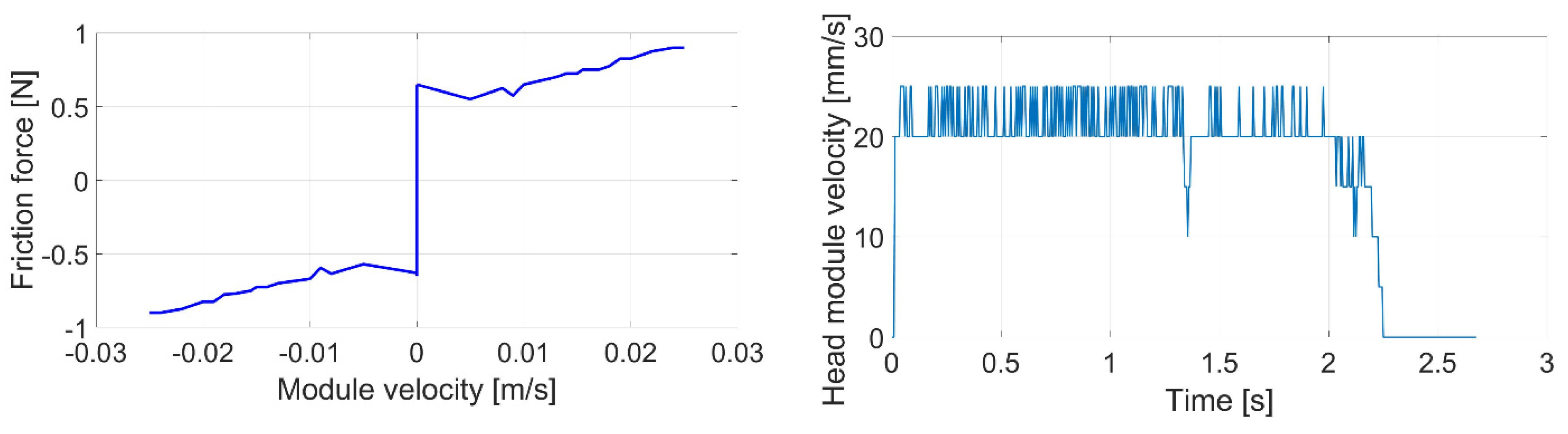
Next, the experiment was performed on a surface with a layer of oil. The results are shown in Figure 17.
With increasing snake robot module velocity, friction also increased, indicating the viscous friction model + Coulomb friction model. The resultant friction characteristic was roughly symmetrical again. For the next experiment, there was a layer of lubricant on the pipe surface. The results are shown in Figure 18.
As before, the resultant friction characteristic was roughly symmetrical. We can conclude these experiments by stating that the resultant friction characteristics of all measurements offered an almost symmetrical shape.
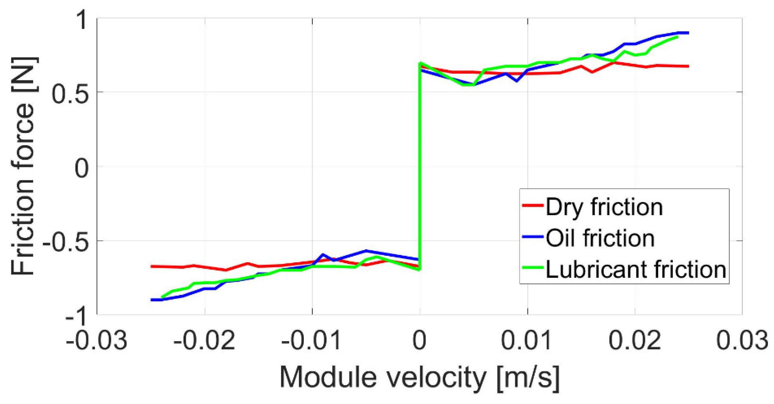
Figure 19 presents the combination of all measurements of friction.
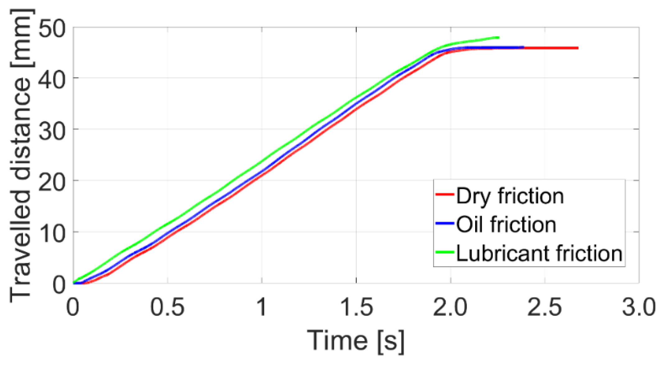
Measured friction forces were almost the same for both directions of module motion. The following experiments show the traveled distance of one module with the different kinds of surfaces. The results are shown in Figure 20. It is obvious that the results were very similar, with only small deviations.
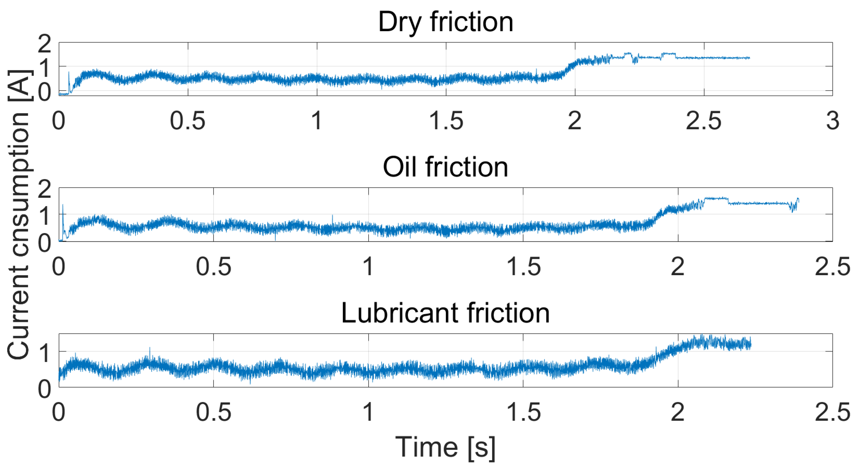
Figure 21 shows the results of measured electrical current consumption during linear motion of the head module. On the basis of these results, there were no significant differences between dry, oil, and lubricant surfaces. Figure 22 shows the snake robot module during its motion on the lubricant surface. A certain layer of the lubricant caused faster linear motion in comparison with dry friction.
The results of these experiments can be summarized as follows. With a dry surface under the snake robot module, the resultant friction was according to the Coulomb friction model. A layer of oil or lubricant resulted in the Coulomb friction + viscous friction model or, rather, Stribeck friction model. With respect to the measurement of friction in both directions, the results had symmetrical characteristics. From the point of view of time duration of linear motion, the slowest motion occurred for the dry surface and the fastest motion occurred for the lubricant surface. With regard to electrical current consumption, the three cases were almost the same.
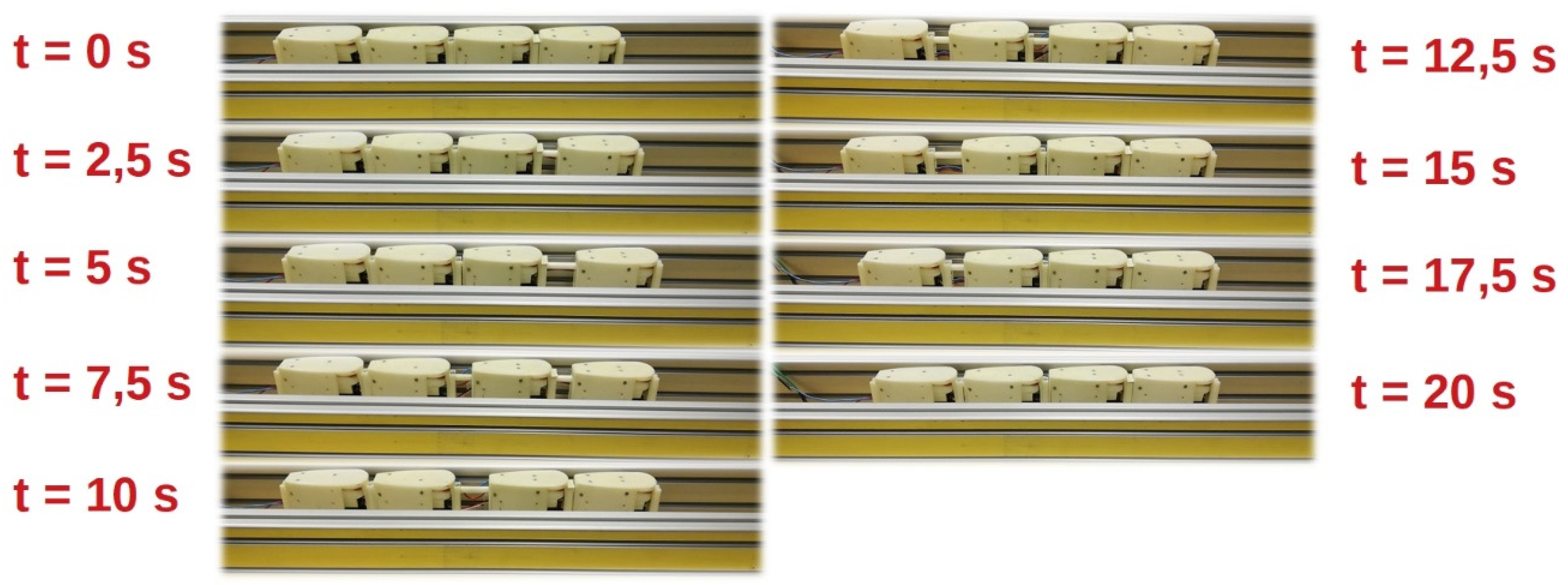
Next, we performed rectilinear locomotion in a pipe (see Figure 23).
During rectilinear locomotion, only one module moved, while others served as support mass. Experimental results from measuring the motion of the head module on different kinds of surfaces were presented in a previous section. The following results present rectilinear locomotion during three cycles. The robot moved on dry surface, surface with oil, and surface with a layer of lubricant.
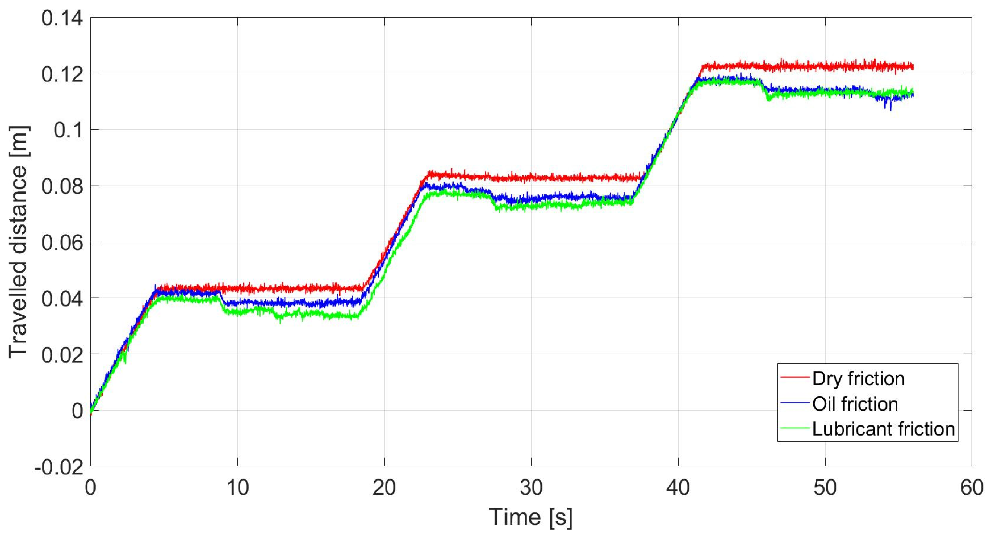
Figure 24 presents the traveled distance of the head module during three locomotion cycles. During locomotion linear protrusion was used for all linear servomotors. The experimental results were quite interesting. With dry friction, the snake robot traveled the maximum possible distance. However, with oil and lubricant, we can see some decrease in traveled distance. In both cases, after the head module traveled its path, during the subsequent motion of other modules, the snake robot started to slide backward under the influence of forces between the modules. This resulted in less traveled distance. That is, real applications need to consider the influence of the environment, which, as we can see, could have an impact on locomotion properties.
6.3. Experimental Analysis of Stability
Section 3 presented the locomotion pattern of the snake robot moving in a pipe. The locomotion was based on anchoring certain modules between the walls of the pipe, while other modules moved freely in the direction of motion. The introduced locomotion pattern considered anchored modules to have a triangular curved shape (see Figure 3). Of course, anchoring of modules between pipe walls could be used in several ways. Our approach assumed different curves that could be formed by the body of the snake robot. It was clear that the more modules the snake robot had, the more precisely the body could form the chosen curve.
The aim of this section is to investigate how the different curves formed by the discrete body of the snake robot affected concertina locomotion stability. In other words, the snake robot used different kinds of anchoring during concertina locomotion, and we investigated if these ways of anchoring were suitable for locomotion. That is, the following section discusses three symmetrical curves that were applied for anchoring of modules during locomotion and were experimentaly analyzed by the DIC method. The snake robot moved through the rectangular and circular pipe while the slope of the pipe was changed. Our focus was on analyzing whether these anchoring curves were able to hold the snake robot in the pipe.
6.3.1. Mathematical Background of Symmetrical Curves
The concept of symmetrical curves relates in our case to the rear modules of the robot, which were used to anchor it between the pipe walls. We chose the following curves due to their rough applicability to our snake robot having eight modules [27].
Triangular Curve
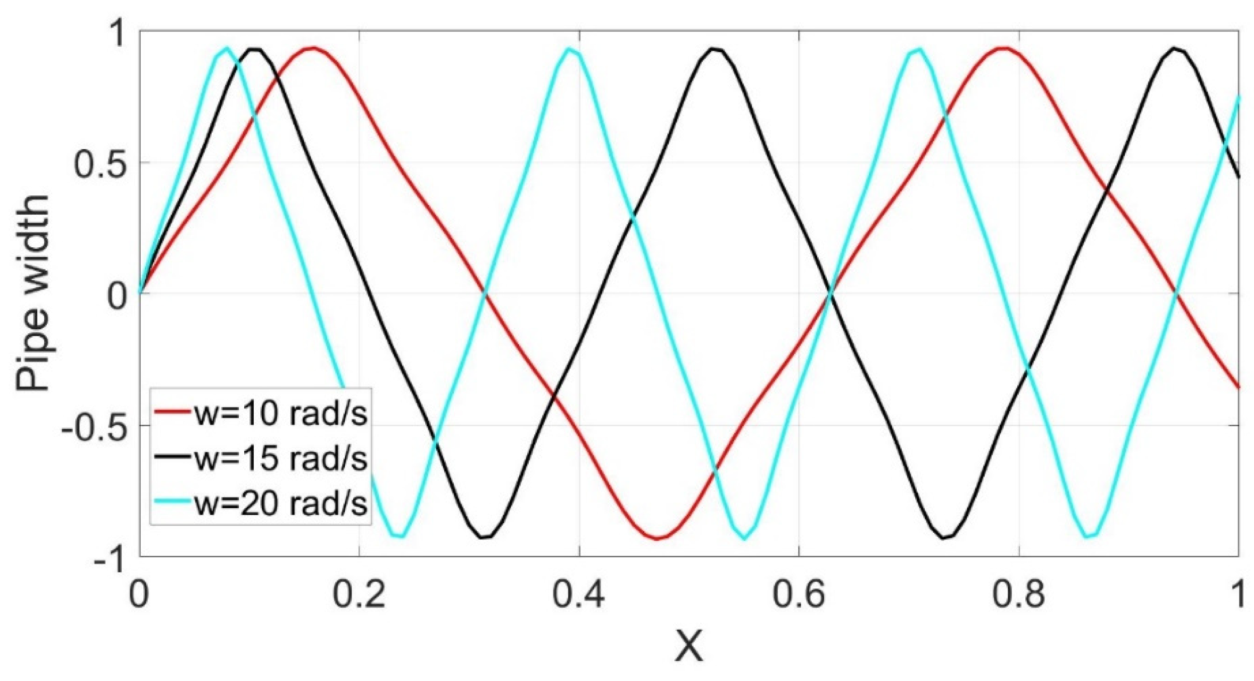
The triangular curve can be described by Equation (9):
where ω is angular frequency. Figure 25 shows three triangular curves with different frequencies. The amplitude of these curves was based on the pipe diameter D. As can be seen, decreasing frequency caused expansion of the curve. The magnitude of frequency depended on the length of the snake robot module. The longer the module, the lower the frequency of the curve.
Cycloid Curve
The cycloid curve can be described by Equation (10):
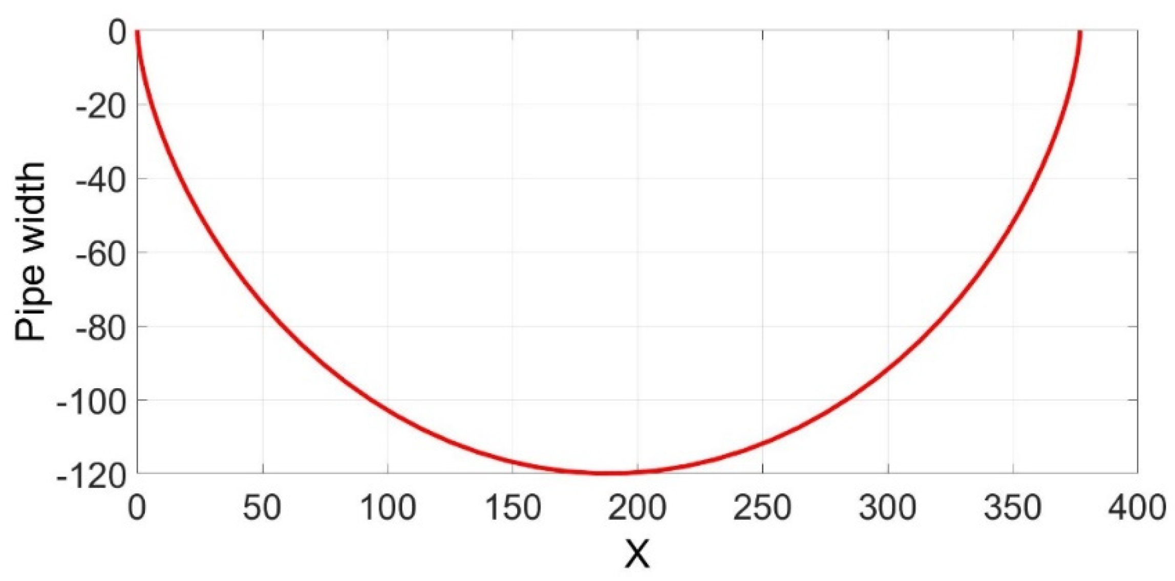
where is the radius of the curve. Figure 26 shows the cycloid curve described by Equation (10). From Equation (10), it is obvious that this curve could be influenced by its radius . From this reason, radius was set according to pipe diameter D.
However, there was a way to shorten or lengthen the cycloid curve by using the following parametric expression:
where denotes shortening or expanding of the cycloid curve. If , the curve was shortened, and if , the curve was expanded.
Gaussian curve
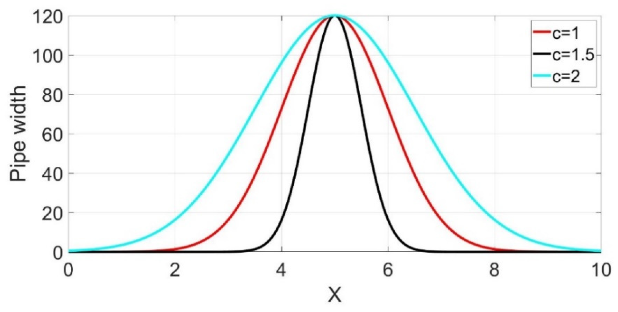
The Gaussian curve is expressed by Equation (12):
where ; represents pipe diameter D, represents the coordinate system origin shift, and represents the change of angle between two robot modules in contact with the wall of the pipe. In other words, parameter shows how “sharp” the Gaussian curve will be (see Figure 27).
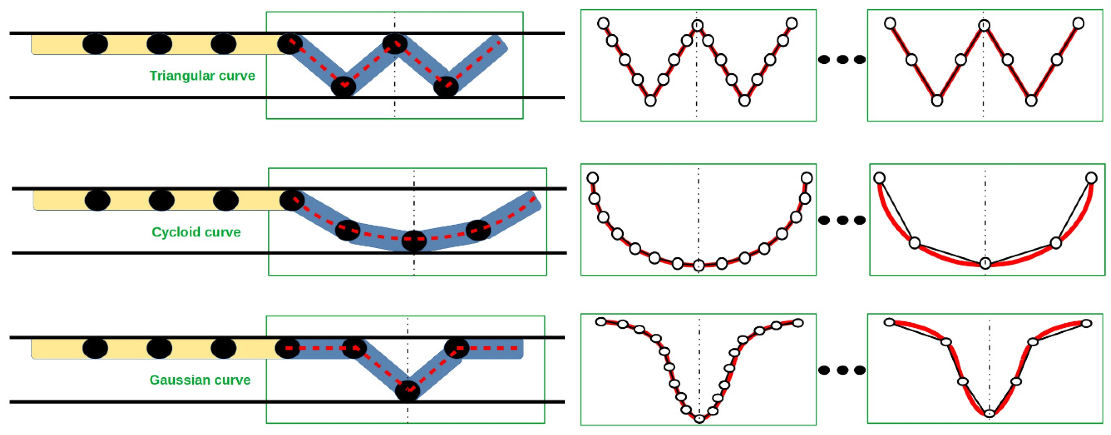
These symmetrical curves were applied to the snake robot body (see Figure 28). In general, by considering the fact that a hyper-redundant mechanism consisted of many of the same modules, we could apply robot modules to these curves. However, we used a snake robot consisting of eight modules (with four for anchoring), and hence it was not possible to precisely copy these curves, which was not even the goal. We could use only rough approximations of these curves. Let us consider Figure 28. In this figure, anchored modules are denoted in gray, and dashed vertical lines represent the axis of symmetry for discrete application of symmetrical curves for rear anchored modules.
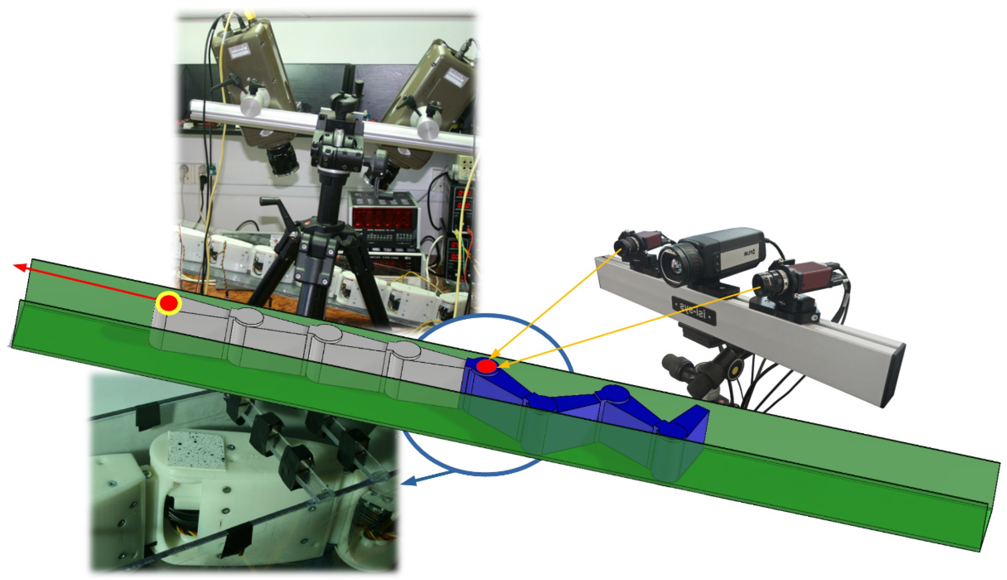
6.3.2. Digital Image Correlation Method
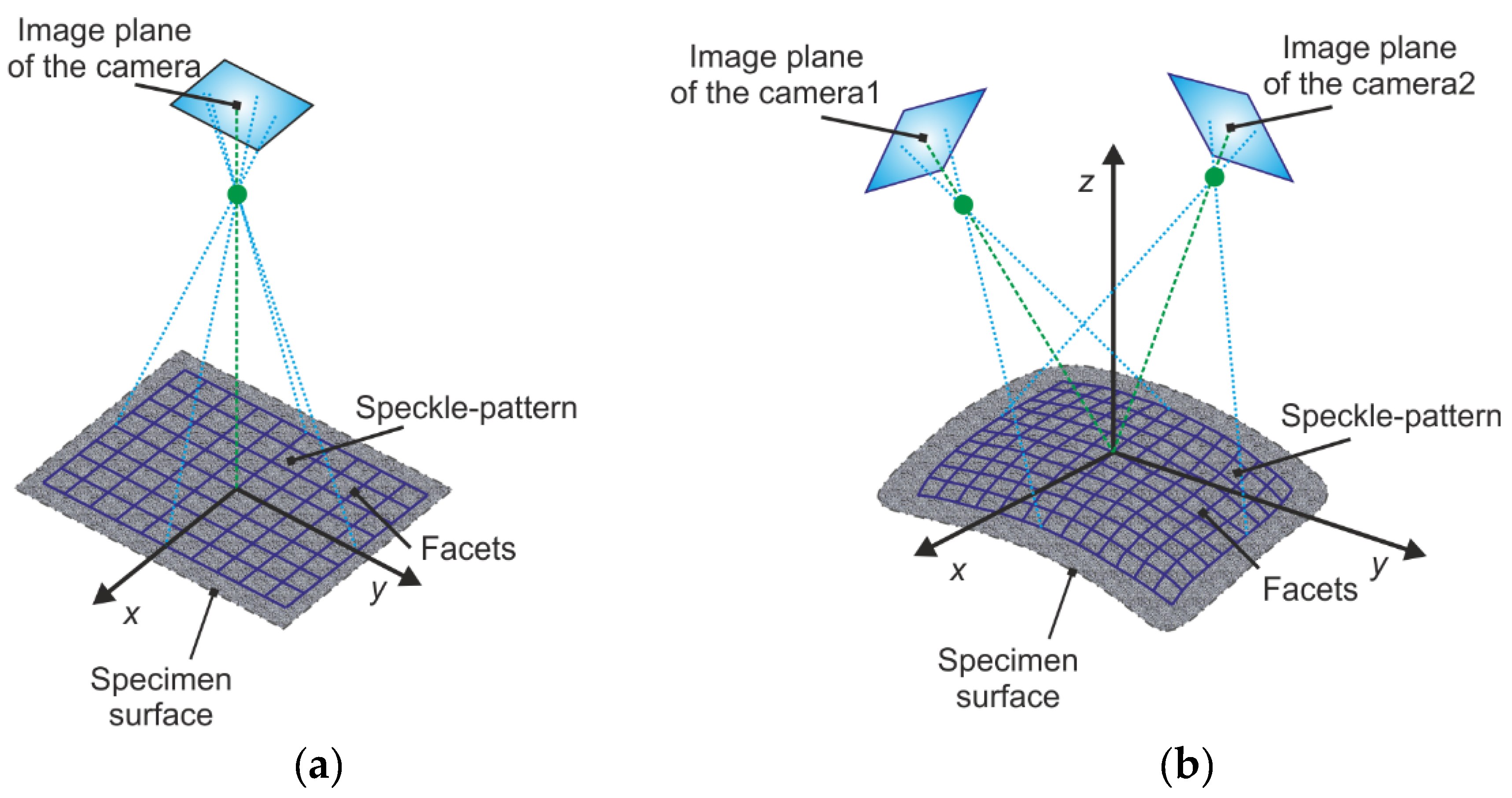
Digital image correlation allowed us to perform measurements commonly using a single or stereo camera system. When the measurement was done with a single camera (see Figure 29a), it was possible to perform only two-dimensional (2D) displacement/deformation analysis. However, it was necessary to ensure that the surface of the investigated object would be parallel to the camera image plane during the whole measurement process. Using a correlation system with stereoscopically arranged cameras (Figure 29b), this condition was not valid and the results were in the form of three-dimensional displacement/deformation fields.
We carried out all described measurements with a commercial Q-450 Dantec Dynamics high-speed digital image correlation system, the technical specifications of which are listed in Table 1. The system consists of two SpeedSense 9070 cameras with CMOS sensors allowing maximal image resolution of 1 Mpx (1080 × 800 px). Optimal light conditions were assured by the use of a special high-power halogen lamp with natural light and frequency of 70 kHz.
The principle of the Dantec Dynamics correlation system is based on the correlation of images along small elements called facets. The standard size of facets is from 15 × 15 px up to 30 × 30 px. As a measuring point, the center of the facet is considered.
To obtain the transform coordinates of each object surface point, the digital image correlation system used a modern approach based on the pseudo-affine transform. If denotes the transform parameters of potential translation, stretch, shear, and distortion of the facet, then using the algorithm, the transform coordinates and can be expressed by Equation (13):
The unknown parameters can be determined by minimizing the difference between the gray value intensity of the points on deformed image and reference image via
where and are the illumination parameters. If all object point coordinates are determined, then the 3D coordinates of the surface are obtained.
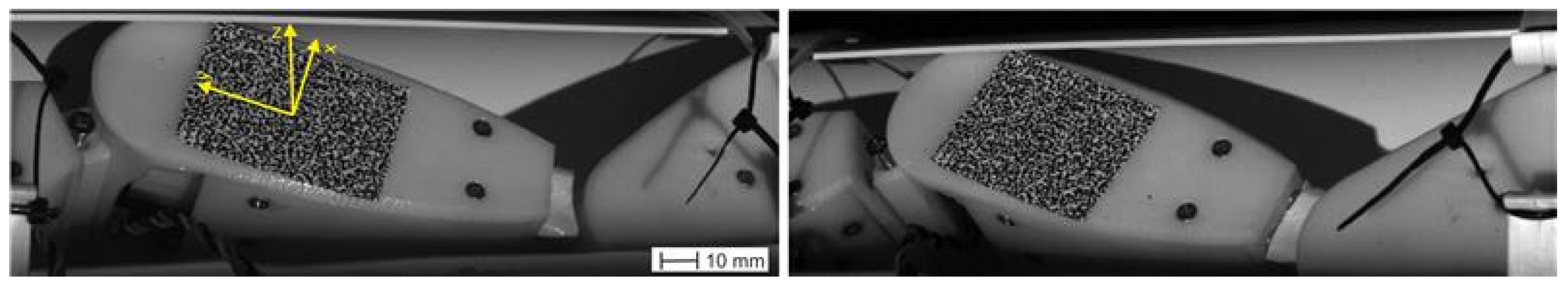
Reference images with a resolution of 1280 × 448 px (density equal to 6 px/mm) captured by the Q-450 Dantec Dynamics 3D correlation system are depicted in Figure 30. The cameras were calibrated by a calibration target with 9 × 9 black and white fields with a field size of 8 × 8 mm. The facet size used for evaluating the measurement was 17 × 17 px and the facets overlaid themselves in 5 px.
6.3.3. Measurement of Stability by DIC Method
The introduced symmetrical curves were experimentally analyzed. The snake robot performed forward motion by linear joints and subsequently the stability of anchored modules was tested using triangular, cycloid, and Gaussian curves. For experimental analysis, the DIC method was used. The measuring method is shown in Figure 31.
As Figure 31 shows, a measuring pattern was stuck to one static (anchored) snake robot module. The aim was to observe the displacement of this module while free modules moved forward.
The conditions of the experiment were as follows. We tested the three mentioned symmetrical curves on surfaces with slopes of 0°, 10°, 20°, and 30°. The measurements were done for two kinds of pipe, one with a rectangular cross-section, and one with a circular cross-section. For each measurement, supply voltage of 4V DC and 8V DC was used. Of course, with a supply voltage of 8V DC for servomotors, the results would have better characteristics. The reason for using 4V DC was that lower electrical current consumption would be required during locomotion. This solution would be suitable for real applications, such as long-time inspection of pipes without an available external voltage supply, whereas the robot would be dependent on batteries.
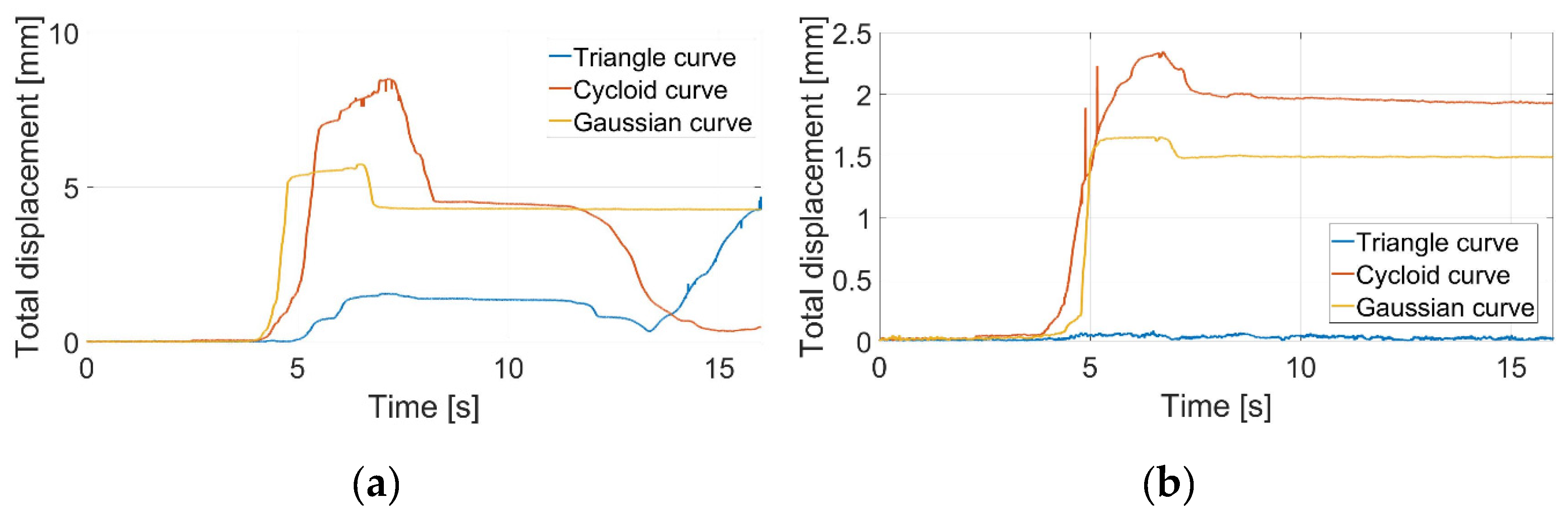
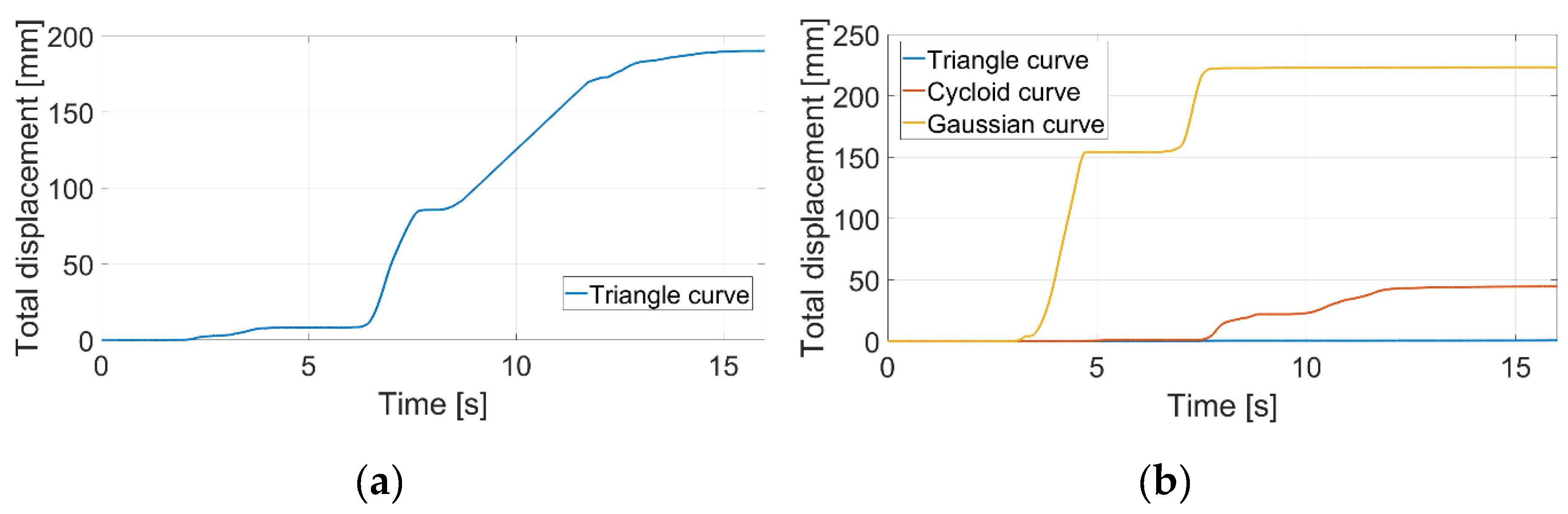
First, we present the results of the experiment with pipes with a rectangular cross-section, shown in Figure 32, Figure 33, Figure 34 and Figure 35.
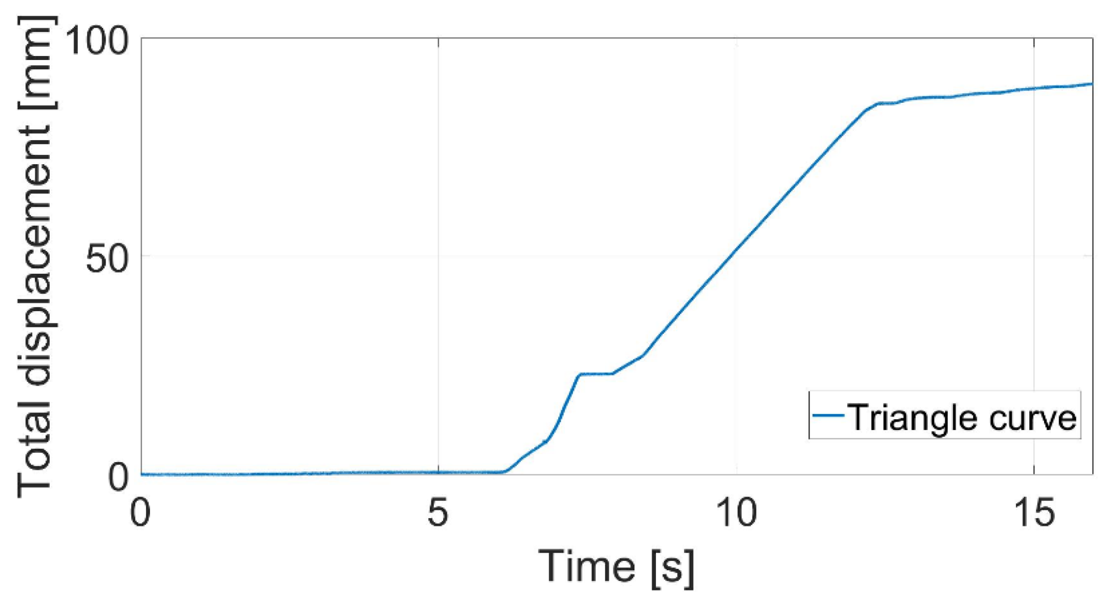
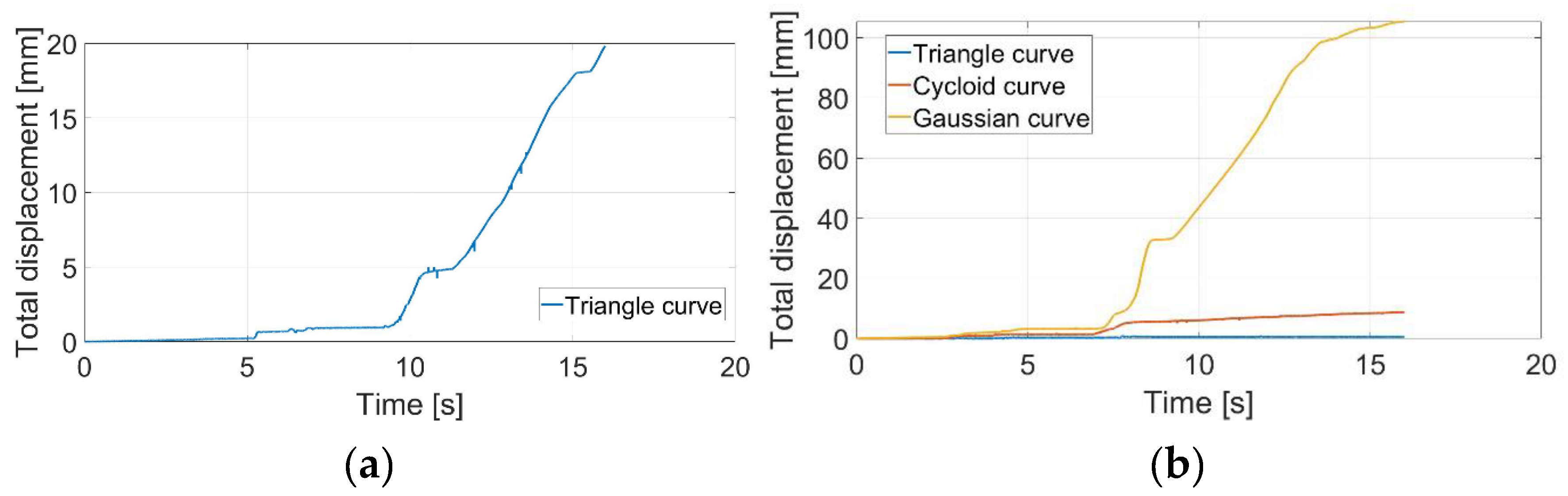
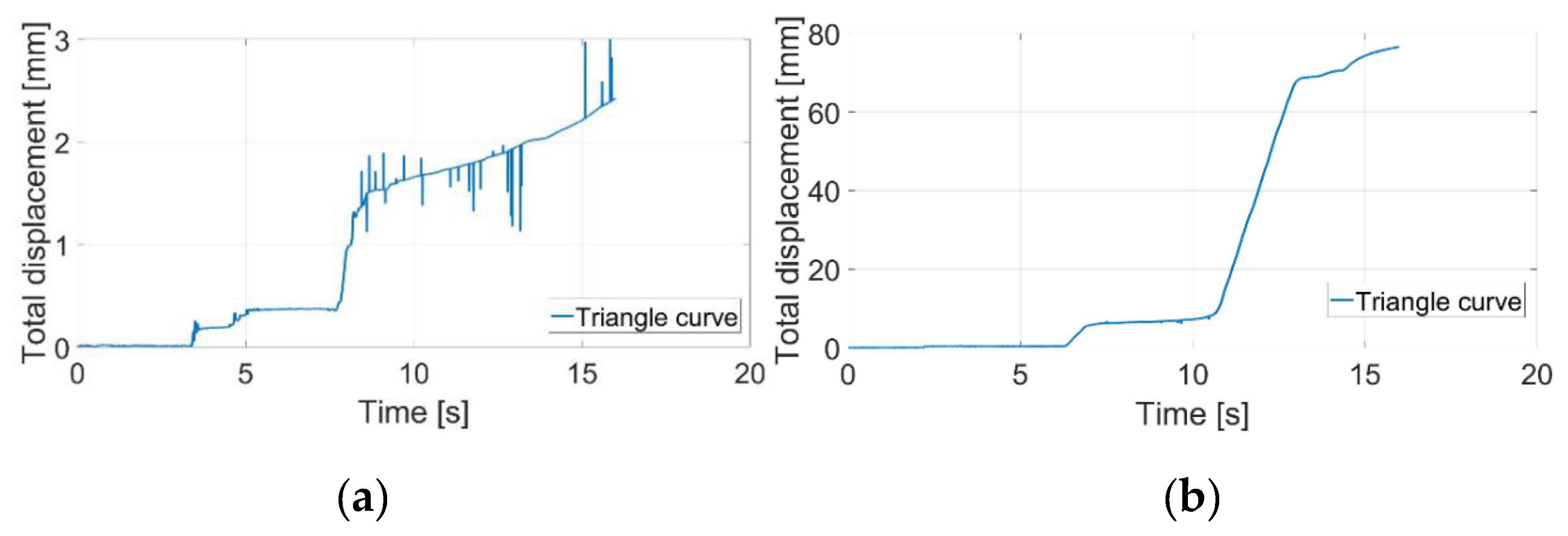
Considering the slope of the surface to be 0°, both graphs showed satisfactory displacement. The snake robot would be able to perform locomotion. In the case of surface slope of 10° and supply voltage of 4V DC, applying cycloid and Gaussian curves, the snake robot slid down and was not able to perform forward locomotion (see Figure 33a). Only the triangular curve was satisfactory. From Figure 33b, it was obvious that the Gaussian curve failed. Because the results of cycloid and Gaussian curves using 4V DC were unsatisfactory, only the triangular curve with 4V DC was measured. In the case of surface slope of 20° and supply voltage of 4V DC, the triangular curve also failed (see Figure 34a). Assuming 8V DC, only the triangular curve was stable (see Figure 34b). In the case of surface slope of 30° and supply voltage of 8V DC, the triangular curve also failed (see Figure 35).
From all measurements of pipe with rectangular cross-section, it was clear that for anchoring of certain snake robot modules, the best solution was to use a triangular curve with supply voltage of 8V DC.
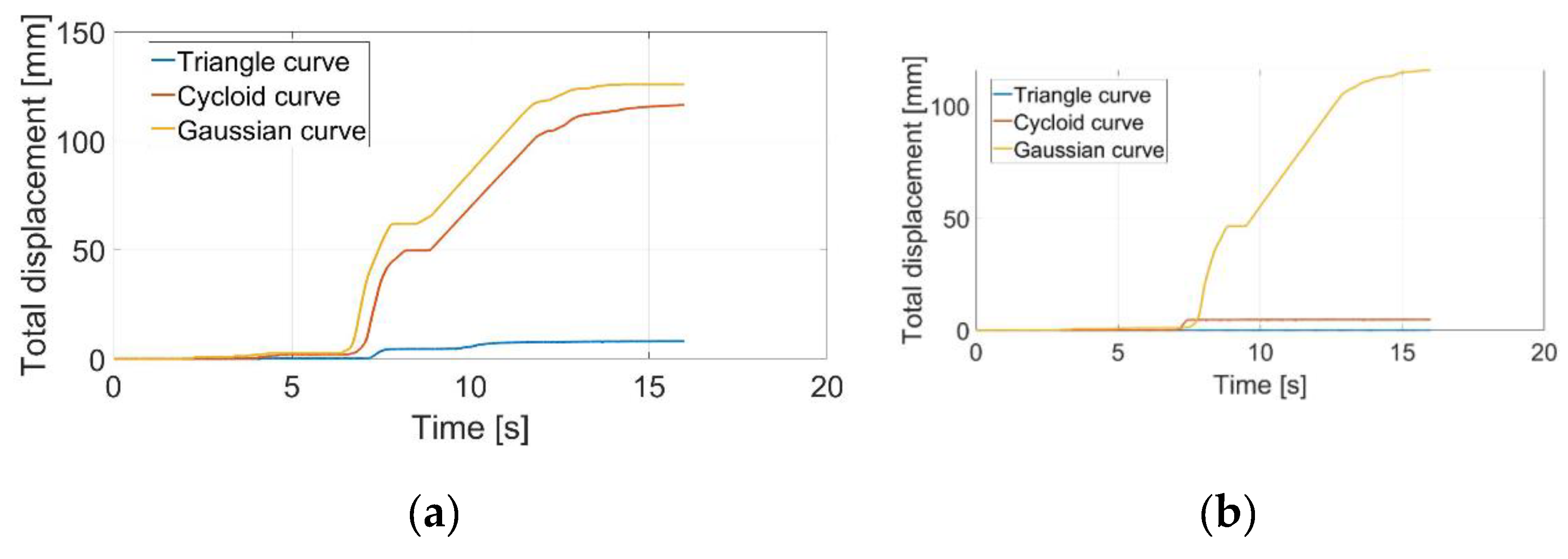
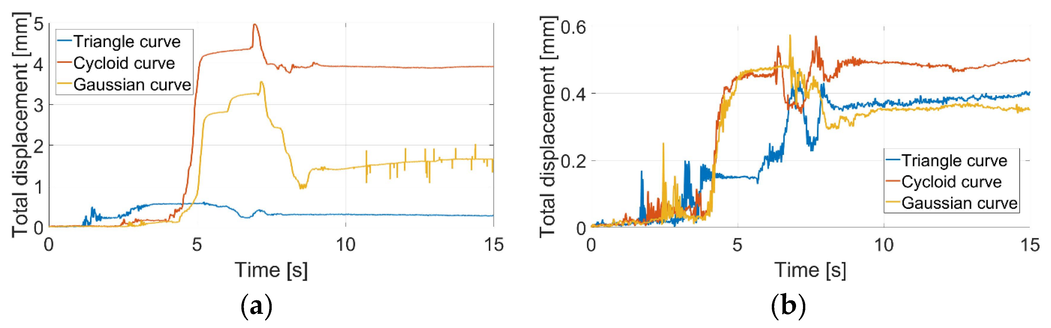
The next measurements relate to pipes with a circular cross-section. The results are shown in Figure 36, Figure 37, Figure 38 and Figure 39.
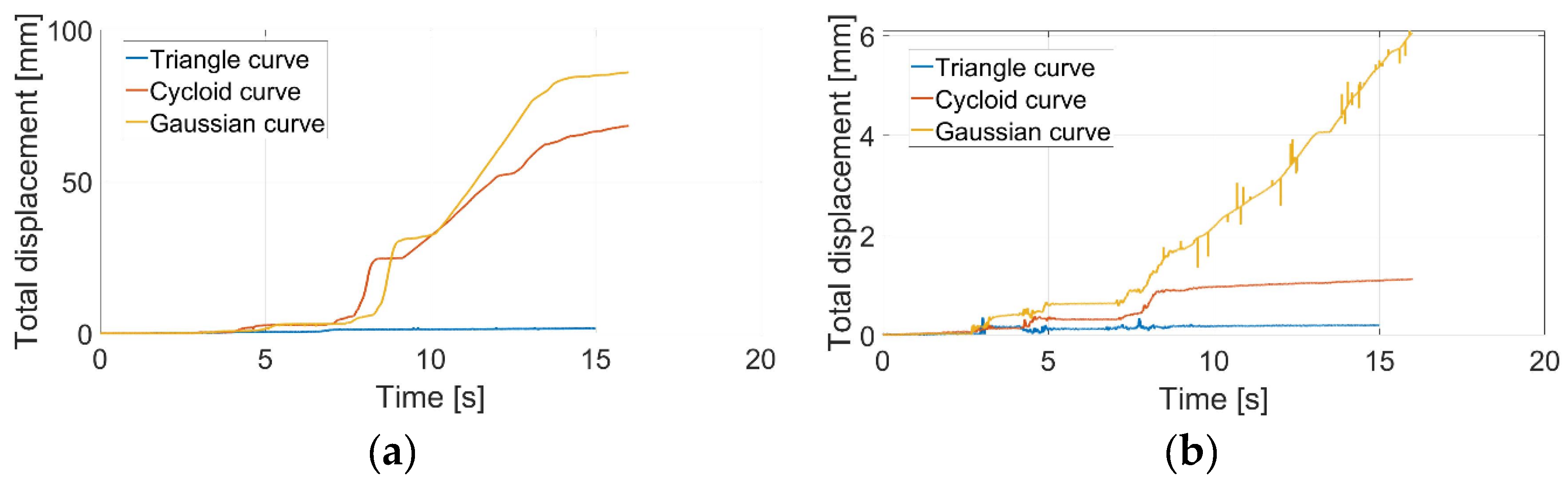
Considering the slope of the surface to be 0°, both graphs showed stable results for locomotion (see Figure 36). By increasing the slope to 10° and using a supply voltage of 4V DC, only the triangular curve gave stable results. One difference between pipes with circular and rectangular cross-sections was in the case of the 10° slope and 8V DC. Although the Gaussian curve failed in the rectangular pipe, in the circular pipe it was a stable solution (see Figure 37b). Another difference was the case of slope 20° and 4V DC. In the circular pipe, the triangular curve was quite successful, whereas in the rectangular it failed (see Figure 38a). In the case of 20° slope and 8V DC, the cycloid curve was quite stable in comparison with the rectangular pipe (see Figure 38b). Assuming a slope of 30° and 8V DC, the triangular curve was still stable (Figure 39a) and for this reason we also measured for a slope of 40°. However, in this case, the triangular curve also failed (see Figure 39b).
The experiments with symmetrical curves used for anchoring snake robot modules between the walls of a pipe can be evaluated as follows. From the perspective of stability, the best solution was to use a triangular curve. The worst solution was the Gaussian curve. Considering the use of the snake robot in real applications with the requirement of low energy intensity, it would not be a satisfactory solution. The robot would be able to perform locomotion only on a horizontal plane. With increased surface slope, stability significantly decreased. Comparing locomotion in rectangular and circular pipes, the snake robot showed significantly better stability in the circular pipe. Whereas in the rectangular pipe some curves failed, in the circular pipe they were still stable.
7. Conclusions
This paper analyzed snake robot locomotion in a pipe. First, we designed a locomotion pattern using revolute and linear joints in the snake robot modules. Subsequently, we verified the pattern by simulation in MATLAB R2015b. Then we introduced our newly developed experimental snake robot. Its uniqueness lay in its combination of revolute and linear joints in one module. This snake robot performed a series of experiments described in this paper. First of all, we verified the designed locomotion pattern by moving the snake robot in a pipe with a rectangular cross-section. Considering real applications of the snake robot in pipes, in which there could be sludge on the pipe surface, we tested its rectilinear locomotion on different kinds of surfaces: dry, with oil, and with lubricant. Next, the experiment was concerned with locomotion of the snake robot in pipes with circular and rectangular cross-sections. Three symmetrical curves were used for anchoring certain modules between the walls of the pipe. We experimentally analyzed the individual symmetrical curves in terms of their stability under the influence of changed slope of the pipe. The DIC method was used for these experiments. The contributions of the paper are as follows:
- Design of concertina locomotion based on revolute and linear joints of snake robot module. Design of mathematical model and analysis of the influence of input parameters.
- Development of a unique experimental snake robot consisting of eight modules, each with one revolute and one linear joint.
- Simulation and experimental analysis of proposed concertina locomotion.
- Experimental analysis of snake robot locomotion on different types of surfaces: dry, with a layer of oil, and with a layer of lubricant. Measured friction in both directions for all cases led to almost symmetrical characteristics. The results showed that electrical current consumption for all cases was almost the same. The robot traveled its maximum possible distance with dry friction. However, with oil or lubricant on the surface, some modules slid backward, resulting in less traveled distance per three locomotion cycles.
- A new approach based on anchoring of snake robot modules during locomotion in a pipe by means of symmetrical curves. Experimental analysis of their stability with changing slope of the pipe by modern DIC methodology using Q-450 Dantec Dynamics high-speed correlation system. The best solution was the use of a triangular curve. The circular pipe offered better stability for snake robot locomotion in the pipe.
The contributions of the paper are unique. This study fills a gap in the area of snake robot locomotion in a confined space such as a pipe or channel.
Author Contributions
Analysis, programming, simulations, and experiments: I.V. and E.P.; experiments: M.K. and M.V.; DIC experiments: M.H.; mechanical design of snake robot: Z.B. and P.O.; supervision and conceptualization: P.B. All authors have read and agreed to the published version of the manuscript.
Funding
This research was funded by Slovak Grant Agency VEGA 1/0389/18 “Research on kinematically redundant mechanisms”. This work was also supported by the European Regional Development Fund in the Research Centre of Advanced Mechatronic Systems project, project number CZ.02.1.01/0.0/0.0/16_019/0000867, within the Operational Programme Research, Development and Education. The work was also funded by research project VEGA 1/0019/20 and is sponsored by project 013TUKE-4/2019: Modern educational tools and methods for forming creativity and increasing practical skills.
Acknowledgments
The authors would like to thank the Slovak Grant Agency VEGA 1/0389/18 “Research on kinematically redundant mechanisms”. This work was also supported by the European Regional Development Fund in the Research Centre of Advanced Mechatronic Systems project, project number CZ.02.1.01/0.0/0.0/16_019/0000867 within the Operational Programme Research, Development and Education. The work was also funded by research project VEGA 1/0019/20 and was sponsored by project 013TUKE-4/2019: Modern educational tools and methods for forming creativity and increasing practical skills.
Conflicts of Interest
The authors declare no conflict of interest. The funders had no role in the design of the study; in the collection, analyses, or interpretation of data; in the writing of the manuscript; or in the decision to publish the results.
References
- Lipták, T.; Virgala, I.; Frankovský, P.; Šarga, P.; Gmiterko, A.; Baločková, L. A geometric approach to modeling of four- and five-link planar snake-like robot. Int. J. Adv. Robot. Syst. 2016, 13. [Google Scholar] [CrossRef]
- Ostertag, O.; Ostertagová, E.; Kelemen, M.; Kelemenová, T.; Virgala, I.; Buša, J. Miniature Mobile Bristled In-Pipe Machine. Int. J. Adv. Robot. Syst. 2014, 11, 189. [Google Scholar] [CrossRef]
- Kelemen, M.; Virgala, I.; Lipták, T.; Ľubica, M.; Filakovský, F.; Bulej, V. A Novel Approach for a Inverse Kinematics Solution of a Redundant Manipulator. Appl. Sci. 2018, 8, 2229. [Google Scholar] [CrossRef] [Green Version]
- Hirose, S. Biologically Inspired Robots: Snake-Like Locomotors and Manipulators; Oxford University Press: Oxford, UK, 1993. [Google Scholar]
- Wakimoto, S.; Nakajima, J.; Takata, M.; Kanda, T.; Suzumori, K. A micro snake-like robot for small pipe inspection. In Proceedings of 2003 International Symposium on Micromechatronics and Human Science (IEEE Cat. No.03TH8717); Institute of Electrical and Electronics Engineers (IEEE): Piscataway, NJ, USA, 2004. [Google Scholar]
- Greenfield, A.; Rizzi, A.A.; Choset, H. Dynamic Ambiguities in Frictional Rigid-body Systems with Application to Climbing via Bracing. In Proceedings of the 2005 IEEE International Conference on Robotics and Automation; Institute of Electrical and Electronics Engineers (IEEE): Piscataway, NJ, USA, 2006; pp. 1947–1952. [Google Scholar]
- Brunete, A.; Gambao, E.; Torres, J.; Hernando, M. A 2 DoF Servomotor-based Module for Pipe Inspection Modular Micro-robots. In Proceedings of the 2006 IEEE/RSJ International Conference on Intelligent Robots and Systems; Institute of Electrical and Electronics Engineers (IEEE): Piscataway, NJ, USA, 2006; pp. 1329–1334. [Google Scholar]
- Barazandeh, F.; Bahr, B.; Moradi, A. How self-locking reduces actuators torque in climbing snake robots. In Proceedings of the 2007 IEEE/ASME International Conference on Advanced Intelligent Mechatronics; Institute of Electrical and Electronics Engineers (IEEE): Piscataway, NJ, USA, 2007; pp. 1–6. [Google Scholar]
- Wright, C.; Johnson, A.M.; Peck, A.; Mccord, Z.; Naaktgeboren, A.; Gianfortoni, P.; Gonzalez-Rivero, M.; Hatton, R.; Choset, H. Design of a modular snake robot. In Proceedings of the 2007 IEEE/RSJ International Conference on Intelligent Robots and Systems; Institute of Electrical and Electronics Engineers (IEEE): Piscataway, NJ, USA, 2007; pp. 2609–2614. [Google Scholar]
- Kuwada, A.; Wakimoto, S.; Suzumori, K.; Adomi, Y. Automatic pipe negotiation control for snake-like robot. In Proceedings of the 2008 IEEE/ASME International Conference on Advanced Intelligent Mechatronics; Institute of Electrical and Electronics Engineers (IEEE): Piscataway, NJ, USA, 2008; pp. 558–563. [Google Scholar]
- Andruska, A.M.; Peterson, K.S. Control of a Snake-Like Robot in an Elastically Deformable Channel. IEEE/ASME Trans. Mechatron. 2008, 13, 219–227. [Google Scholar] [CrossRef]
- Akbarzadeh-T, M.-R.; Safehian, J.; Safehian, J.; Kalani, H. Generating Snake Robot Concertina Locomotion Using a New Dynamic Curve. Int. J. Model. Optim. 2011, 1, 134–140. [Google Scholar] [CrossRef]
- Marvi, H.; Hu, D.L. Friction enhancement in concertina locomotion of snakes. J. R. Soc. Interface 2012, 9, 3067–3080. [Google Scholar] [CrossRef] [PubMed] [Green Version]
- Kano, T.; Satake, F.; Date, H.; Inoue, K.; Ishiguro, A. Doing Well in Narrow Aisle! Decentralized Control Mechanism Underlying Adaptive Concertina Locomotion of Snakes. Int. Symp. Nonlinear Theory Appl. 2014, 32–35. [Google Scholar] [CrossRef]
- Trebuňa, F.; Virgala, I.; Pástor, M.; Lipták, T.; Ľubica, M. An inspection of pipe by snake robot. Int. J. Adv. Robot. Syst. 2016, 13. [Google Scholar] [CrossRef]
- Virgala, I.; Kelemen, M.; Prada, E.; Surovec, R. Motion analysis of snake robot segment. In Proceedings of the 2013 IEEE 11th International Symposium on Applied Machine Intelligence and Informatics (SAMI), Herl’any, Slovakia, 31 January–2 February 2013; pp. 145–148. [Google Scholar] [CrossRef]
- Tang, C.; Shu, X.; Meng, D.-Y.; Zhou, G. Arboreal concertina locomotion of snake robots on cylinders. Int. J. Adv. Robot. Syst. 2017, 14. [Google Scholar] [CrossRef] [Green Version]
- Huang, C.-W.; Huang, C.-H.; Hung, Y.-H.; Chang, C.-Y. Sensing pipes of a nuclear power mechanism using low-cost snake robot. Adv. Mech. Eng. 2018, 10. [Google Scholar] [CrossRef]
- Gray, J. The mechanism of locomotion in snakes. J. Exp. Boil. 1946, 23, 101–120. [Google Scholar]
- Virgala, I.; Kelemen, M.; Varga, M.; Kuryło, P. Analyzing, Modeling and Simulation of Humanoid Robot Hand Motion. Procedia Eng. 2014, 96, 489–499. [Google Scholar] [CrossRef] [Green Version]
- Bozek, P.; Ivandić, Ž.; Lozhkin, A.; Lyalin, V.; Tarasov, V. Solutions to the characteristic equation for industrial robot’s elliptic trajectories. Teh. Vjesn.-Tech. Gaz. 2016, 23, 1017–1023. [Google Scholar] [CrossRef]
- Krolczyk, G.M.; Legutko, S. Experimental Analysis by Measurement of Surface Roughness Variations in Turning Process of Duplex Stainless Steel. Metrol. Meas. Syst. 2014, 21, 759. [Google Scholar] [CrossRef]
- Huang, S.; Liang, W.; Tan, K.K. Intelligent Friction Compensation: A Review. IEEE/ASME Trans. Mechatron. 2019, 24, 1763–1774. [Google Scholar] [CrossRef]
- Virgala, I.; Frankovský, P.; Frankovský, M.K.P.; Kenderová, M. Friction Effect Analysis of a DC Motor. Am. J. Mech. Eng. 2013, 1, 1–5. [Google Scholar] [CrossRef] [Green Version]
- Liu, L.; Xu, W.; Yue, X.-L.; Huang, D. Stochastic Bifurcation of a Strongly Non-Linear Vibro-Impact System with Coulomb Friction under Real Noise. Symmetry 2018, 11, 4. [Google Scholar] [CrossRef] [Green Version]
- Yamada, S. Nanotribology of Symmetric and Asymmetric Liquid Lubricants. Symmetry 2010, 2, 320–345. [Google Scholar] [CrossRef] [Green Version]
- Prada, E.; Valášek, M.; Virgala, I.; Gmiterko, A.; Kelemen, M.; Hagara, M.; Lipták, T.; Erik, P. New approach of fixation possibilities investigation for snake robot in the pipe. In Proceedings of the 2015 IEEE International Conference on Mechatronics and Automation (ICMA); Institute of Electrical and Electronics Engineers (IEEE): Piscataway, NJ, USA, 2015; pp. 1204–1210. [Google Scholar]
Figure 1.
Block diagram of investigation of snake robot locomotion possibilities.

Figure 2.
Corn snake concertina locomotion [13]
Figure 2.
Corn snake concertina locomotion [13]

Figure 3.
Locomotion pattern in a pipe.

Figure 4.
Traveled distance of snake robot based on pipe diameter and linear joint protrusion.

Figure 5.
Traveled distance based on change of pipe diameter.

Figure 6.
Snake robot locomotion in rectangular pipe using concertina and rectilinear locomotion patterns.
Figure 6.
Snake robot locomotion in rectangular pipe using concertina and rectilinear locomotion patterns.

Figure 7.
Time courses of snake robot joints during locomotion.

Figure 8.
Snake robot modules a) Revolute motion of module b) Linear motion of module.

Figure 9.
Kinematic configuration of snake robot modules.

Figure 10.
Inside of snake robot module.

Figure 11.
CAD model (top) and experimental snake robot (bottom).

Figure 12.
Snake robot module data flow.

Figure 13.
Locomotion in a pipe.

Figure 14.
Traveled distance of head module during concertina locomotion.

Figure 15.
Friction models: (a) Coulomb (without static friction), (b) Coulomb + viscous friction (without static friction), (c) stiction + Coulomb + viscous friction, (d) Stribeck.
Figure 15.
Friction models: (a) Coulomb (without static friction), (b) Coulomb + viscous friction (without static friction), (c) stiction + Coulomb + viscous friction, (d) Stribeck.

Figure 16.
Clean surface of pipe.

Figure 17.
Surface with oil.

Figure 18.
Surface with lubricant.

Figure 19.
All measured surfaces.

Figure 20.
Traveled distance of snake robot module on different kinds of surfaces.

Figure 21.
Electrical current consumption during motion of head module.

Figure 22.
Layer of lubricant on the surface.

Figure 23.
Rectilinear locomotion of snake robot.

Figure 24.
Rectilinear locomotion on different surfaces.

Figure 25.
Triangular curves.

Figure 26.
Cycloid curve.

Figure 27.
Gaussian curves.

Figure 28.
Anchoring of snake robot rear by three symmetrical curves.

Figure 29.
Scheme of (a) single-camera (2D) and (b) stereo camera (3D) correlation system.

Figure 30.
Typical reference images captured by Q-450 Dantec Dynamics high-speed digital image correlation system.
Figure 30.
Typical reference images captured by Q-450 Dantec Dynamics high-speed digital image correlation system.

Figure 31.
Measuring anchoring possibilities of snake robot during its motion.

Figure 32.
Pipe with rectangular cross-section and slope 0°: (a) supply voltage 4V DC, (b) supply voltage 8V DC.
Figure 32.
Pipe with rectangular cross-section and slope 0°: (a) supply voltage 4V DC, (b) supply voltage 8V DC.

Figure 33.
Pipe with rectangular cross-section and slope 10°: (a) supply voltage 4V DC, (b) supply voltage 8V DC.
Figure 33.
Pipe with rectangular cross-section and slope 10°: (a) supply voltage 4V DC, (b) supply voltage 8V DC.

Figure 34.
Pipe with rectangular cross-section and slope 20°: (a) supply voltage 4V DC, (b) supply voltage 8V DC.
Figure 34.
Pipe with rectangular cross-section and slope 20°: (a) supply voltage 4V DC, (b) supply voltage 8V DC.

Figure 35.
Pipe with rectangular cross-section and slope 30°: triangle fixation curve, supply voltage 8V DC.
Figure 35.
Pipe with rectangular cross-section and slope 30°: triangle fixation curve, supply voltage 8V DC.

Figure 36.
Pipe with circular cross-section and slope 0°: (a) supply voltage 4V DC, (b) supply voltage 8V DC.
Figure 36.
Pipe with circular cross-section and slope 0°: (a) supply voltage 4V DC, (b) supply voltage 8V DC.

Figure 37.
Pipe with circular cross-section and slope 10°: (a) supply voltage 4V DC, (b) supply voltage 8V DC.
Figure 37.
Pipe with circular cross-section and slope 10°: (a) supply voltage 4V DC, (b) supply voltage 8V DC.

Figure 38.
Pipe with circular cross-section and slope 20°: (a) supply voltage 4V DC, (b) supply voltage 8V DC.
Figure 38.
Pipe with circular cross-section and slope 20°: (a) supply voltage 4V DC, (b) supply voltage 8V DC.

Figure 39.
Pipe with circular cross-section and supply voltage 8V DC with (a) slope 30°, (b) slope: 40°.
Figure 39.
Pipe with circular cross-section and supply voltage 8V DC with (a) slope 30°, (b) slope: 40°.


Table 1.
Technical specifications of Q-450 Dantec Dynamics high-speed cameras used for experimental analysis.
Table 1.
Technical specifications of Q-450 Dantec Dynamics high-speed cameras used for experimental analysis.
| Field of view | Adjustable from several mm2 to several m2 Typical size from 70 × 50 mm2 to 400 × 300 mm2 |
| Measuring range | Displacement: ≈10–5 of field of view (100 mm field corresponds to 1 μm) |
| Exposure time | Adjustable from 300 ns |
| Resolution | Max. 1280 × 800 px up to sampling frequency of 3140 fps |
| Results form | 3D contour of analyzed object, 3D displacement |
| Control electronics | Laptop with Windows 7 and Istra4D control software, 16-bit AD/DA converter (eight channels with voltage range from ±0.05 V to ±10 V) |
| Illumination | High-power halogen lamp with natural light |
© 2020 by the authors. Licensee MDPI, Basel, Switzerland. This article is an open access article distributed under the terms and conditions of the Creative Commons Attribution (CC BY) license (http://creativecommons.org/licenses/by/4.0/).
Share and Cite
MDPI and ACS Style
Virgala, I.; Kelemen, M.; Božek, P.; Bobovský, Z.; Hagara, M.; Prada, E.; Oščádal, P.; Varga, M. Investigation of Snake Robot Locomotion Possibilities in a Pipe. Symmetry 2020, 12, 939. https://doi.org/10.3390/sym12060939
AMA Style
Virgala I, Kelemen M, Božek P, Bobovský Z, Hagara M, Prada E, Oščádal P, Varga M. Investigation of Snake Robot Locomotion Possibilities in a Pipe. Symmetry. 2020; 12(6):939. https://doi.org/10.3390/sym12060939
Chicago/Turabian StyleVirgala, Ivan, Michal Kelemen, Pavol Božek, Zdenko Bobovský, Martin Hagara, Erik Prada, Petr Oščádal, and Martin Varga. 2020. "Investigation of Snake Robot Locomotion Possibilities in a Pipe" Symmetry 12, no. 6: 939. https://doi.org/10.3390/sym12060939
Note that from the first issue of 2016, this journal uses article numbers instead of page numbers. See further details here.