A Double-Density Clustering Method Based on “Nearest to First in” Strategy

Abstract

The existing density clustering algorithms have high error rates on processing data sets with mixed density clusters. For overcoming shortcomings of these algorithms, a double-density clustering method based on Nearest-to-First-in strategy, DDNFC, is proposed, which calculates two densities for each point by using its reverse k nearest neighborhood and local spatial position deviation, respectively. Points whose densities are both greater than respective average densities of all points are core. By searching the strongly connected subgraph in the graph constructed by the core objects, the data set is clustered initially. Then each non-core object is classified to its nearest cluster by using a strategy dubbed as ‘Nearest-to-First-in’: the distance of each unclassified point to its nearest cluster calculated firstly; only the points with the minimum distance are placed to their nearest cluster; this procedure is repeated until all unclassified points are clustered or the minimum distance is infinite. To test the proposed method, experiments on several artificial and real-world data sets are carried out. The results show that DDNFC is superior to the state-of-art methods like DBSCAN, DPC, RNN-DBSCAN, and so on.

1. Introduction

How to dig unknown information out of data sets is a widely concerned problem. Clustering, as an unsupervised method to partition a data set naturally, has the ability to discover the potential and internal knowledge, laws and rules of data. In recent decades, researchers have proposed many clustering algorithms based on different theories and models, which are generally divided into several categories such as partitioning, hierarchical, density, grid and model based methods. [1]

K-Means [2], a famous partitioning based clustering method, is suitable to the data set composed of spherical clusters, even though the clusters have different densities. One of the limitations of K-Means is that it unfits for the data sets having arbitrary shape clusters. Agglomerative [3] is a type of hierarchical clustering using button-up approach and Ward’s linkage, the method for calculating the distance between clusters, is its most commonly used method for its good monotonicity and spatial expansion. The time complexities of hierarchical clustering methods are often high. Meanshift [4] is a general non-parametric clustering method and suitable to data sets with arbitrary shape clusters.

Density-based clustering is famous for its capability of finding out arbitrary shape clusters from data sets and therefore it has been widely used in data mining, pattern recognition, machine learning, information retrieval, image analysis and other fields in recent years [5,6,7,8,9,10,11,12,13,14,15,16].

Ester etc. proposed a density-based algorithm for discovering clusters in large spatial databases with noise (DBSCAN) [17] in 1996, and since then lots of density-based clustering have been proposed and used widely. DBSCAN needs two parameters: eps and minpts. The density of each point is estimated by counting the number of points in its hypersphere with eps radius and each point then is recognized as a core or non-core object according to whether its density is greater than minpts or not. An obvious weakness of DBSCAN is that it is very difficult to select two appropriate parameters for different data sets. Rodriguez and Laio proposed a new clustering approach by fast search and find of density peaks (DPC) [18]. It is simpler and more effective than DBSCAN because only one parameter is needed and the clustering centers can be selected in a visible mode by projecting points into the $\rho -ϵ$ decision graph. But DPC cannot partition a data set with adjacent clusters of different densities correctly. For improving the performance of DPC, many methods tried to update the density calculation, mode of clustering centers selection, and so on. Vadapalli etc. introduced reverse k nearest neighbors (RNN) model into density-based clustering (RECORD) [19] and adopted the same way as DBSCAN to define the reachability of points in a data set but only required one parameter k. Though RECORD often confuses the points lying on borders of clusters with noises, for its ability to detect the cores of clusters with different densities correctly, some improved methods have been proposed.

The density-based approaches mentioned above are using only one way to measure point densities in the data set. So, though they performed well on data sets with arbitrary shape but separately distributing clusters, they cannot partition low-density clusters from their adjacent high-density clusters in mixture-density data sets. In this paper, a density clustering method based on double density and Nearest-to-First-in strategy is proposed, which is dubbed as DDNFC. Compared with the above state-of-the-art density clustering algorithms, this method has the following advantages: (1) It can depict the distributions of data in a data set more accurately by using the two densities of each point, reverse k-nearest neighbor number and local offset of position; (2) According to the two densities and respective thresholds, a data set is divided initially into several core areas with high-density points and a low-density boundary surrounding them. In this way, the low density clusters are not over segmented easily; (3) Adapting the Nearest-to-First-in strategy, only those unclassified boundary points closest to the existing clusters are classified in each iteration, and then the sensitivity of clustering to the input parameter and the impact of storage order of data points on classification results are reduced.

The remainder of this paper is organized as follows. In Section 2, we redefined the core object, which is introduced in DBSCAN firstly, and give the procedure of clustering the core objects initially. Moreover, the complexity of initial clustering procedure was analyzed here. Section 3 described Nearest-to-First-in strategy proposed by this paper in detail. We also analyzed the complexity of the strategy in this section. In Section 4, experimental results on synthetic and real data sets are presented and discussed. Additionally, the choice of appropriate of k is under discussion in this section. Finally, conclusions are made in Section 5.

2. Core Objects and Initial Clustering

In this section, we give two densities to represent the distribution of data, introduce and improve some notations defined in DBSCAN and RECORD into this paper but improve them, describe the Nearest-to-First-in strategy.

2.1. Abbreviations

X: a data set with N d-dimension points;

$|\cdot |$: the counting function to calculate the size of a set;

$x,y,z$: three points in the data set X;

$d(x,y)$: a distance function returns a real value of the distance between points x and y, it is the Euclidean function in this paper;

k: the input parameter indicates the number of nearest neighbors of an point;

$N_k\left(x\right)$: the set of k nearest neighborhoods of point x;

$R_k\left(x\right)$: the set of reverse k nearest neighbors of point x, which is defined as $R_k\left(x\right):=\left\{y\right|y\in X\&x\in N_k\left(y\right)\}$;

c: the number of clusters in data set X;

$C_i,C_j$: the $i^{th}$ and $j^{th}$ clusters, $1\le i,j\le c,i\ne j,C_i\cap C_j=\varnothing$;

L: label array, in which, the value of each element indicates the cluster the corresponding point belongs to.

2.2. Density of Each Point

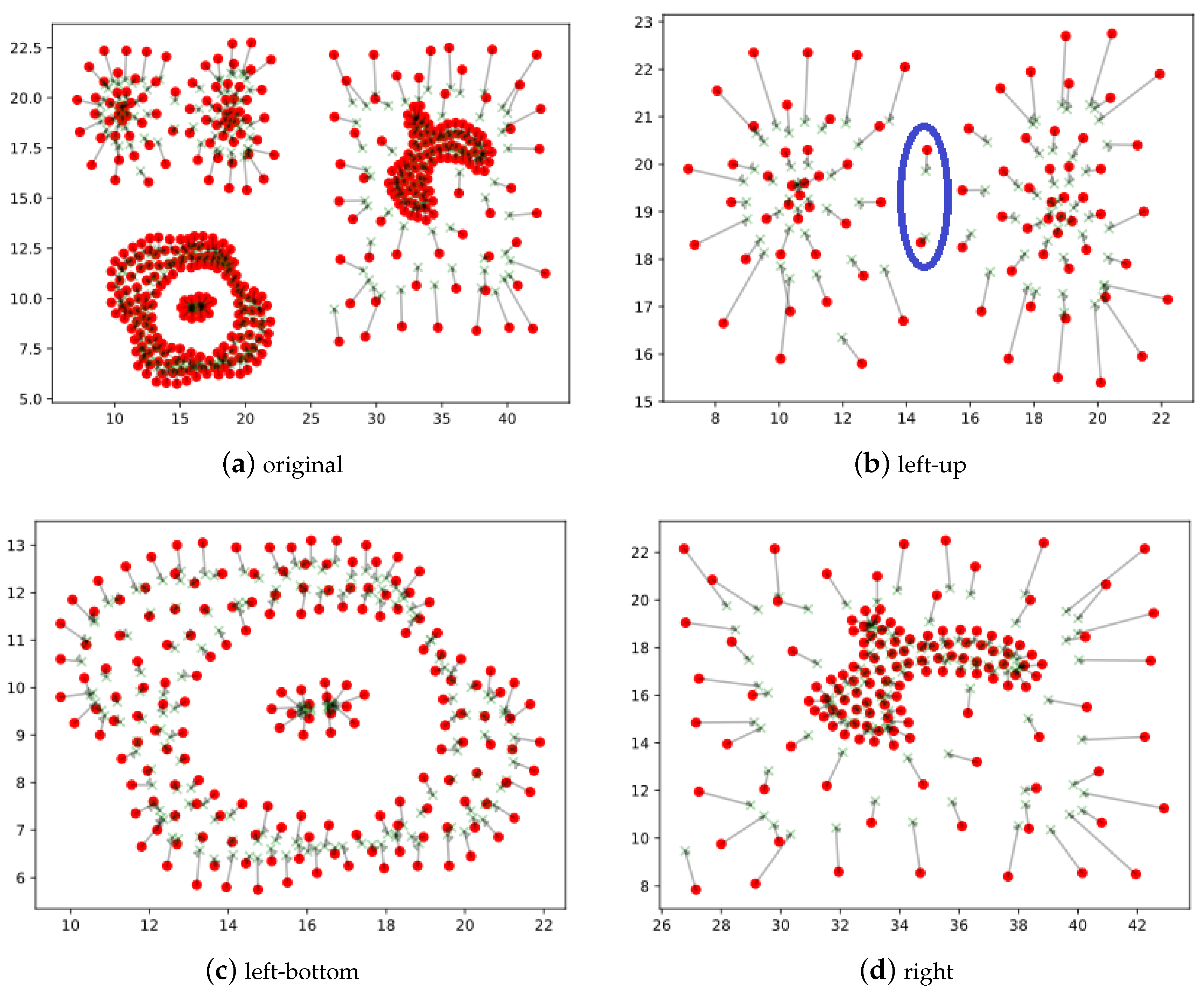
In some cases, using only one density cannot portray the real distribution of data. For example, as shown in Figure 1, Compound [20] is a typical data set composed of several clusters with different shapes and densities, and the clusters are adjacent or surrounded each other. Dividing it into correct clusters is a difficult task. In this paper, we use two densities to detect the true core areas of clusters. For each point in a data set, apart from using the reverse k nearest neighbors model to compute density, we introduce the offset of local position of a point to calculate its another density.

Definition 1.

Offset of local position. The offset of local position of point x is the distance between x and the geometric center $\overline{x}$ of all its k nearest neighbors, which is defined as follows:

$$d_{off}\left(x\right)=d(x,\overline{x})$$

(1)

where $\overline{x}=\frac{1}{k}{\sum }_{y\in N_k\left(x\right)}y$.

As displayed in Figure 1, the original position of each point is a red ball in the figure, and the semi-transparent green cross connected with it is the geometrical center of its k nearest neighborhoods, and the length of line connected a red ball and its corresponding green cross with directed arrow is the offset of local position. Figure 1a is the entire view of points and their offsets of Component, and Figure 1b–d are the partial view of Compound. From these figures, we can find the truth that the value of offset of an point is small when it lies in the central of local region but is large in the boundary, and the sparser the data distributed locally, the larger the offset is. So it is reasonable to estimate density of the point by using the offset of local position. But it also has defects, as shown in Figure 1b, the two boundary points, which are circled out by a blue ellipse, have very small offset values because they locate in the local center of their neighbors. We use two density computing methods to estimate the true distribution of a point in the data set and they are defined as follows: (1) Density computed by the offset of local position

$${\rho }_{off}\left(x\right)=exp\left(-d_{off}^2\left(x\right)\right)$$

(2)

(2) Density computed by the reverse k nearest neighbors model

$${\rho }_R\left(x\right)=\left|R_k\left(x\right)\right|$$

(3)

2.3. Core Object

By the two densities of all points, two corresponding thresholds are set, and then we are able to classify each point into two types: core or non-core.

Definition 2.

Core object. A point x in data set X is a core object if it satisfies the following condition:

$${\rho }_{off}\left(x\right)>\frac{1}{N}\sum _{y\in X}{\rho }_{off}\left(y\right)and{\rho }_R\left(x\right)\ge k$$

(4)

Those points that do not satisfy the above condition are non-core objects.

After extracting core objects from a data set, we improve the two relationships, density directly-reachable and density reachable, which were defined in DBSCAN firstly. By these relations we construct a directed graph and find its maximum connected components, which contain the cores of all clusters.

Definition 3.

Density directly-reachable. A point x is density directly-reachable from another point y if they satisfy the two conditions as follows:

(1) x and y are all core objects;

(2) $x\in R_k\left(y\right)$.

Because that x is one of reverse k nearest neighbors of y is not able to guarantee y is the reverse k nearest neighbor to x, too, y is not definitely density directly-reachable from x. It is to say that the density directly-reachable is not symmetrical.

Definition 4.

Density reachable. A point x is density reachable from another point y if there are a series of points, $x_1,\dots ,x_m$ and $x=x_1,y=x_m$, satisfying the following conditions:

(1) $\forall i,1\le i\le m,x_i$ is a core object;

(2) $\forall i,1\le i<m,x_i$ is density directly-reachable from $x_{i+1}$. The density reachable is not symmetrical for density directly-reachable being unsymmetrical.

2.4. Initial Clustering

In Algorithm 1, instead of constructing a directed graph of core objects obviously, we randomly start from an unclassified core object and visit all unclassified core objects density directly-reachable or reachable relationship from the point classified before, and the procedure is implemented iteratively.

Algorithm 1: Initial clustering.

Input: data set X, k, $N_k$, $R_k$.

Output: label array L.

Step 1. Initialize each element of L to 0, and set $Cid$ to 0;

Step 2. for each $x_i$ in X:

Step 3.       Compute $d_{off}\left(x_i\right)$ by (1);

Step 4.       Calculate ${\rho }_{off}\left(x_i\right)$ and ${\rho }_R\left(x_i\right)$ by (2) and (3) respectively;

Step 5. Calculate the threshold ${\overline{\rho }}_{off}$ by (4)

Step 6. for each $x_i$ in X:

Step 7.       if ${\rho }_{off}\left(x_i\right)>{\overline{\rho }}_{off}$ and ${\rho }_R\left(x_i\right)>k$:

Step 8.             $L\left(x_i\right)=-1$

Step 9. Initialize an empty queue Q

Step 10. for each $x_i$ in X:

Step 11.       if $L\left(x_i\right)!=-1$:   continue;

Step 12.       $Q.push\left(x_i\right)$, $Cid+=1$;

Step 13.       while Q is not empty:

Step 14.             $x=Q.pop\left(\right)$, $L\left(x\right)=Cid$;

Step 15.             for each y in $R_k\left(x\right)$:

Step 16.                   if $L\left(y\right)==-1$:   $Q.push\left(y\right)$;

Step 17. return L.

In Algorithm 1, there are $2kN$ spaces to store the elements of $N_k$ and $R_k$. And L, ${\rho }_{off}$ and ${\rho }_R$ need memory spaces N each. The storage spaces for the queue Q are dynamic but not beyond N. Thus the space complexity of the algorithm is $O\left(kN\right)$. The loop needs repeat $kN$ times for calculating the two densities for all point from step 2 to 4 of the algorithm. The times for computing ${\overline{\rho }}_{off}$ in step 5 and finding out all core objects from step 6 to 8 are all N obviously according to the corresponding definition. Steps from 10 to 16 form a three layers nested loop. The most inner loop is steps 15–16. It repeats more than k but less than $2k$ times on average. The iterating times of the second loop depend on how many core objects are density reachable from the original seed point taken in step 11 but obviously are no more than N. The outer loop calls the inner loops c times if the dataset has c core regions. So, the time complexity of the nested loop is $O\left(ckN\right)$. The larger c is, the smaller the core regions will be, then the less time the second loop needs. Finding the k-nearest-neighbor set $N_k$ and the inverse k-nearest-neighbor set $R_k$ of each point before calling the algorithm are the common procedures for all related density-based approaches but do not specially need by our method, so we directly estimate their time complexity $O\left(N^2\right)$. Therefore, the total time complexity of Initial Clustering procedure is $O\left(N^2\right)$.

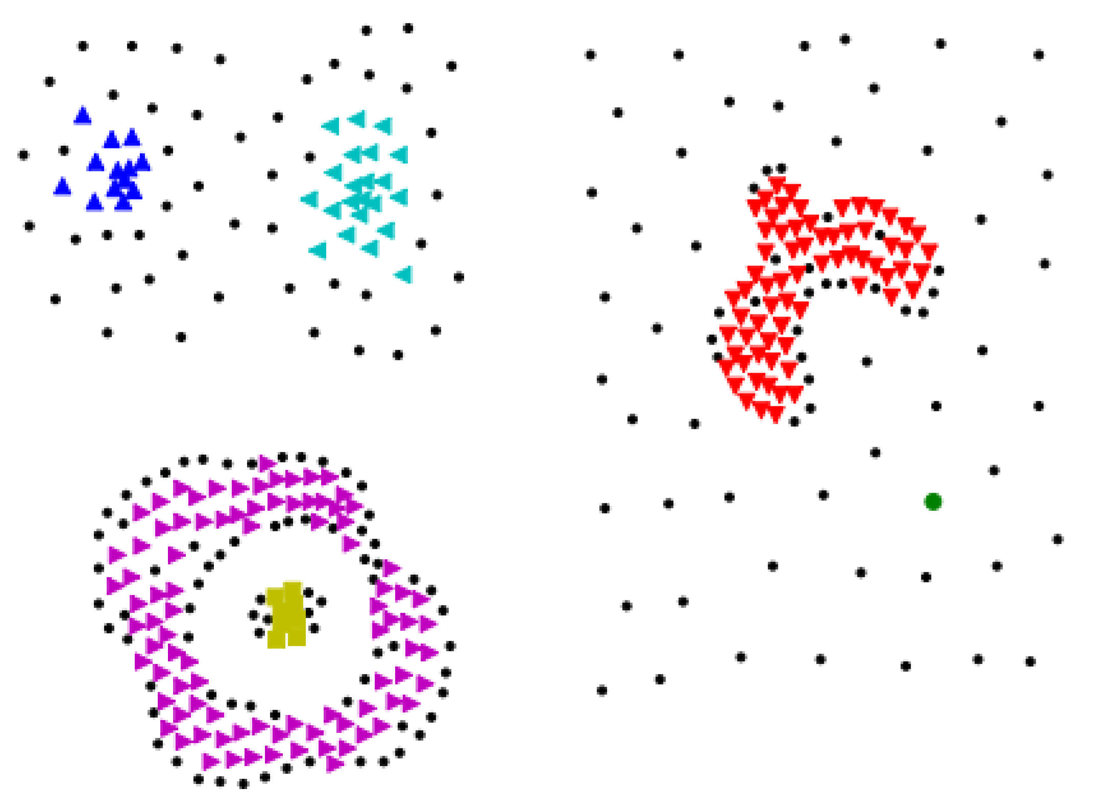
Figure 2 shows the result of initial clustering on data set Compound with $k=7$. Algorithm 1 gets 6 initial clusters. The blue ball in the right-bottom corner is the core object of the right sparse cluster.

3. Nearest-to-First-in Strategy

The initial clustering procedure groups all core objects, while there are a large number of non-core objects unclustered in the data set. Many density-based clustering such as RECORD, IS-DBSCAN, ISB-DBSCAN and RNN-DBSCAN adopted different approaches to classify each non-core object into one of clusters or treat it as noise. But these methods have a weakness that the clustering result suffers from the storage order of points. A Nearest-to-First-in strategy introduced in this section can solve the problem. We illustrate the basic idea and give the implementation steps of the algorithm. Moreover, we analyze the time and space complexity of this strategy.

3.1. Basic Idea of the Strategy

The Nearest-to-First-in Strategy is based on two simple ideas: (1) the closer the points are, the higher the probability is that they belong to the same category; (2) by using the higher probability event priority principle, the cost of clustering will be minimized. To illustrate the advances of our strategy, we first introduce several definitions.

Definition 5.

Distance from an unclassified point to a cluster. The distance between an unclassified point x and a cluster $C_i$, dubbed as $d(x,C_i)$, is defined as:

$$d(x,C_i)=\left\{\begin{array}{cc}{min}_{y\in R_k\left(x\right)\cap C_i}d(x,y),\hfill & if{R}_k\left(x\right)\cap C_i\ne \varnothing \hfill \\ \infty ,\hfill & otherwise\hfill \end{array}\right.$$

(5)

To compute the distance between an unclassified point x and a certain cluster $C_i$, we first check whether the intersection of the reverse k nearest neighbor set $R_k\left(x\right)$ and $C_i$ is empty or not. If the intersection is not empty, which we call x is adjacent to $C_i$, the distance between x and $C_i$ is the distance between x and the point in the intersection nearest to x. Otherwise, the distance from x to $C_i$ is infinite.

Definition 6.

Nearest cluster. Given an unclassified point x, its nearest cluster $C_N\left(x\right)$ is:

$$C_N\left(x\right)={argmin}_{C_i,1\le i\le c}d(x,C_i)$$

(6)

In particular, if x has the same distance to several clusters, even if x is not adjacent to any cluster, $C_N\left(x\right)$ will be set to the first cluster in the ordered list of distances from x.

Definition 7.

Smallest distance to clusters. The smallest distance to clusters $d_{min}$ is the smallest one among the distances from all unclassified points to their nearest cluster respectively, that is:

$$d_{min}={min}_{x\in X,L\left(x\right)=0}d\left(x,C_N\left(x\right)\right)$$

(7)

where $L\left(x\right)$ represents the cluster label of x, its value is 0 if it is unclassified. The value of $d_{min}$ is ∞ if all unclassified points to their nearest clusters are ∞.

Definition 8.

Nearest neighbors of clusters. Given the smallest distance $d_{min}$, the nearest neighbors of clusters $NN$ is defined as follows:

$$NN=\left\{x|x\in X,L\left(x\right)=0,d\left(x,C_N\left(x\right)\right)=d_{min}\right\}$$

(8)

$NN$ is composed all those unclassified points closest to clusters. But $NN$ will be empty if $d_{min}$ is infinite.

3.2. Main Procedures of Nearest-to-First-in Strategy

The Nearest-to-First-in strategy is a greedy strategy. As shown in Algorithm 2, the clustering procedures of the stragtegy for unclassified points are completed in an iterative way. In each iteration, the nearest neighbors of clusters $NN$ is calculated by using (5)–(8), and then the points in the set $NN$ are allocated to their corresponding nearest neighbor clusters. Repeat this process until the $NN$ becomes empty. At this time, either all points have been classified, or the unclassified points are not adjacent to any existing clusters. In this case, the unclassified points will be regarded as noise.

It should be noted that according to Definition 6, getting the nearest cluster of an unclassified point x may be impacted by the storage order of the reverse k nearest neighbor of x, but the Definitions 7 and 8 will minimize this impact.

Algorithm 2: NTFI.

Input: $X,k,R_k,L$.

Output: label array L.

Step 1. Put all unclassified point ($L\left(x\right)=0$) into an array $unL$ and create two array D and $C_N$, each has the same size as $unL$. The value of each element in $C_N$ is set to −1 and the value of each element in D is set to ∞;

Step 2. while $unL$ is not empty:

Step 3.       $d_{min}=\infty$;

Step 4.       for each x in $unL$:

Step 5.             for each y in $R_k\left(x\right)$:

Step 6.                   if $L\left(y\right)>0$ and $dist(x,y)<D\left(x\right)$:

Step 7.                         $D\left(x\right)=dist(x,y),C_N\left(y\right)=L\left(y\right)$;

Step 8.             if $D\left(x\right)<d_{min}$: $d_{min}=D\left(x\right)$;

Step 9.       if $d_{min}=\infty$: break;

Step 10.       for each x in $unL$:

Step 11.             if $D\left(x\right)==d_{min}$:

Step 12.                   $L\left(x\right)=C_N\left(x\right)$;

Step 13.                   Remove x from $unL,D,C_N$;

Step 14. Return L.

In the process of classification, the strategy selects the points with global priority to be processed every time, but classifies them according to the principle of locality, so it can get better cluster results on unclassified points than other density-based clustering.

In the procedure of the Nearest-to-First-in strategy, the main memories needed for running the program are: 1. The distance matrix needs $N^2$ entries of real values. 2. Size of the reverse k nearest neighbors set is $kN$. 3. A label array needs N spaces to indicate the cluster label for each element. 4. Sets of unclassified points such as $unL,D,C_N$ need less than N units each. Therefore, the space complexity of this algorithm is $O\left(N^2\right)$.

In completing the strategy, the number of unclassified points is the key factor in determination of the time complexity, and of course it is less than N. The most time-consuming part is a tree layer nested loop from step 2 to 8, which is used to calculate the nearest cluster $C_N$ and its respective distance D of all unclassified points according to (6) and (5). Obviously, the size of $R_k\left(x\right)$ of an unclassified point x is less than k because x is a non-core object, so the iterative times of the inner two nested loop from step 5 to 7 are less than $kN$. Another inner loop between step 10 and step 13 is to classify those unlabeled points which are nearest to existing clusters and its iterative times also depend on the number of unclassified points. Step 13 removes all newly labelled points in one iteration and then the next loop times will decrease. While step 9 avoid the algorithm not to loop endlessly if there is any point cannot be classified. The total time complexity is $k{N}^2$. In fact, after a round of iteration, it is not necessary to recalculate $C_N$ and D of all the remaining unclassified points. We only need to update the unclassified points in the k nearest neighbor of the new classification points in this round of iteration, so the time required is $k^2$. In the worst case, there is only one unclassified point to be classified in one iteration but iterating N times. Thus, the worst time complexity of this algorithm is $O\left(k^{2}N\right)$.

4. Experiments and Results Analysis

In order to verify the effectiveness of DDNFC, we compare it with another six algorithms, DPC, RNN-DBSCAN [21], DBSCAN, KMeans [2], Ward-link and Meanshift [4], on artificial and real data sets. By using three cluster validity indexes [1,22,23], F-measure with $\alpha =1$ (F1), adjusted mutual information (AMI) and adjusted rand index (ARI), we evaluate and discuss the performances of these seven methods. All algorithms are implemented in Python Integrated Development Environments (version 3.7). DPC and RNN-DBSCAN are coded according to the original articles respectively. Other five methods we use are the built-in algorithms or models provided by scikit-learn library [24]. The ways of parameter setting of the algorithms are described as follows: (1) Meanshift uses the default parameters of the model in scikit-learn; (2) The input parameters of KMeans and Ward-Link are all set to the true number of clusters. KMeans adopts KMeans++ to initialize the centers of clusters; (3) To get the best result of DBSCAN, we use the grid-searching method to find the optimal values for the two parameters, $eps$ and $minpts$. The value of $eps$ varies in the range of 0.1−0.5 and the interval is 0.1. While the $minpts$ ranges from 5 to 30 and steps 5. (4) The cutoff distance required by DPC is calculated by the input percentage value. In this paper, the optimal parameter value is searched from 1.0 to 5.0 percentages in steps of 0.5. In order to simplify the implementation of DPC, we select c points with the top values of $gamma$, which defined as $gamma=\rho *\delta$ in [18], directly as the cluster centers. In addition, the density of DPC is calculated by Gauss kernel. (5) The optimal values of parameter k of our method and RNN-DBSCAN are set in the range of $\left[2\sqrt{N}\right)$.

In addition, spectral clustering [25] is a famous algorithm and has been widely used too. Since it uses k-nearest neighbors to construct an adjacent matrix just as our methods do, we implemented the algorithm on data sets: Spiral, Swiss Roll, Compound, Pathbased, and Aggregation.

4.1. Experiments on Artificial Data Sets and Results Analysis

Table 1. Artificial data sets.

Data Set	Size	Dimension	Cluster Number
Compound	399	2	6
Pathbased	300	2	3
Flame	240	2	2
Aggregation	788	2	7
Jain	373	2	3
R15	600	2	15
Unbalance	6500	2	8
A3	7500	2	50
S1	5000	2	15
t5.8k	8000	2	6
t7.10k	10,000	2	9
t8.8k	8000	2	8
Spiral	312	2	3

displays the basic information of artificial data sets used in the paper. These data sets are all two dimensions and composed of clusters with different densities, shapes and distributed orientations [20,26].

Table 2. Experiment results on artificial data sets.

Algorithm	Par	c/C	F1	AMI	ARI		Par	c/C	F1	AMI	ARI
	Compound						Pathbased
DDNFC	9	6/6	1.00	0.99	1.00		9	3/3	0.98	0.92	0.94
DPC	1.0	6/6	0.78	0.82	0.62		1.5	3/3	0.74	0.55	0.50
RNN-DBSCAN	8	6/6	0.89	0.86	0.86		6	4/3	0.98	0.93	0.95
DBSCAN	0.2/5	6/6	0.94	0.89	0.93		0.3/11	3/3	0.96	0.84	0.88
Ward-Link	6	6/6	0.72	0.69	0.55		3	3/3	0.72	0.53	0.48
KMeans++	6	6/6	0.70	0.68	0.54		3	3/3	0.70	0.51	0.46
MeanShift	-	4/6	0.83	0.74	0.78		-	3/3	0.70	0.51	0.46
	Jain						Flame
DDNFC	18	2/2	1.00	1.00	1.00		17	2/2	1.00	1.00	1.00
DPC	1.0	2/2	0.93	0.61	0.71		4.5	2/2	1.00	0.96	0.98
RNN-DBSCAN	15	2/2	0.99	0.92	0.97		8	2/2	0.99	0.93	0.97
DBSCAN	0.25/14	2/2	1.00	1.00	1.00		0.45/11	3/2	0.99	0.91	0.97
Ward-Link	2	2/2	0.87	0.47	0.51		2	2/2	0.72	0.33	0.19
KMeans++	2	2/2	0.80	0.34	0.32		2	2/2	0.84	0.39	0.45
MeanShift	-	2/2	0.62	0.21	0.02		-	2/2	0.86	0.43	0.50
	cluto-t8.8k						cluto-t7.10k
DDNFC	24	9/9	0.94	0.92	0.95		35	10/10	0.90	0.87	0.89
DPC	1.0	9/9	0.58	0.60	0.48		1.0	10/10	0.55	0.57	0.37
RNN-DBSCAN	22	9/9	0.94	0.91	0.94		35	10/10	0.90	0.87	0.90
DBSCAN	0.1/23	10/9	0.92	0.90	0.91		0.1/8	10/10	0.44	0.28	0.20
Ward-Link	9	9/9	0.49	0.53	0.33		10	10/10	0.55	0.61	0.41
KMeans++	9	9/9	0.52	0.55	0.36		10	10/10	0.47	0.54	0.34
MeanShift	-	7/9	0.51	0.54	0.36		-	6/10	0.54	0.58	0.44
	Aggregation						cluto-t5.8k
DDNFC	6	7/7	0.99	0.99	0.99		34	7/7	0.82	0.79	0.78
DPC	2.0	7/7	1.00	1.00	1.00		2.0	7/7	0.79	0.79	0.74
RNN-DBSCAN	5	7/7	1.00	0.99	0.99		39	7/7	0.82	0.80	0.79
DBSCAN	0.3/23	7/7	0.94	0.91	0.91		0.15/11	7/7	0.28	0.05	0.01
Ward-Link	7	7/7	0.90	0.88	0.81		7	7/7	0.78	0.79	0.74
KMeans++	7	7/7	0.85	0.83	0.76		7	7/7	0.78	0.79	0.74
MeanShift	-	6/7	0.90	0.84	0.84		-	6/7	0.81	0.79	0.78
	Unbalance						R15
DDNFC	63	8/8	1.00	1.00	1.00		24	15/15	0.99	0.99	0.99
DPC	1.0	8/8	1.00	1.00	1.00		1.0	15/15	1.00	0.99	0.99
RNN-DBSCAN	25	8/8	1.00	1.00	1.00		12	15/15	1.00	0.99	0.99
DBSCAN	0.45/11	8/8	0.79	0.70	0.61		0.1/17	15/15	0.76	0.62	0.27
Ward-Link	8	8/8	1.00	1.00	1.00		15	15/15	0.99	0.99	0.98
KMeans++	8	8/8	1.00	1.00	1.00		15	15/15	1.00	0.99	0.99
MeanShift	-	8/8	1.00	1.00	1.00		-	8/15	0.58	0.58	0.27
	S1						A3
DDNFC	29	15/15	0.99	0.99	0.99		36	50/50	0.97	0.97	0.94
DPC	2.5	15/15	0.99	0.99	0.99		1.0	50/50	0.95	0.95	0.91
RNN-DBSCAN	20	16/15	0.99	0.99	0.99		39	49/50	0.97	0.97	0.95
DBSCAN	0.1/8	15/15	0.94	0.93	0.89		0.1/29	37/50	0.78	0.86	0.67
Ward-Link	15	15/15	0.99	0.98	0.98		50	50/50	0.97	0.97	0.94
KMeans++	15	15/15	0.99	0.99	0.99		50	50/50	0.96	0.97	0.94
MeanShift	-	9/15	0.64	0.70	0.56		-	-	-	-	-

Note: The bold numbers in the table indicate the best results the algorithm obtained. The underline numbers mean the algorithm got uncorrect number of clusters.

shows the settings of parameters (dubbed as par) and the test results, such as the number of clusters the methods obtain and the true cluster numbers (dubbed as c/C), the values of F1, AMI and ARI, of the above seven algorithms on artificial and real data sets respectively.

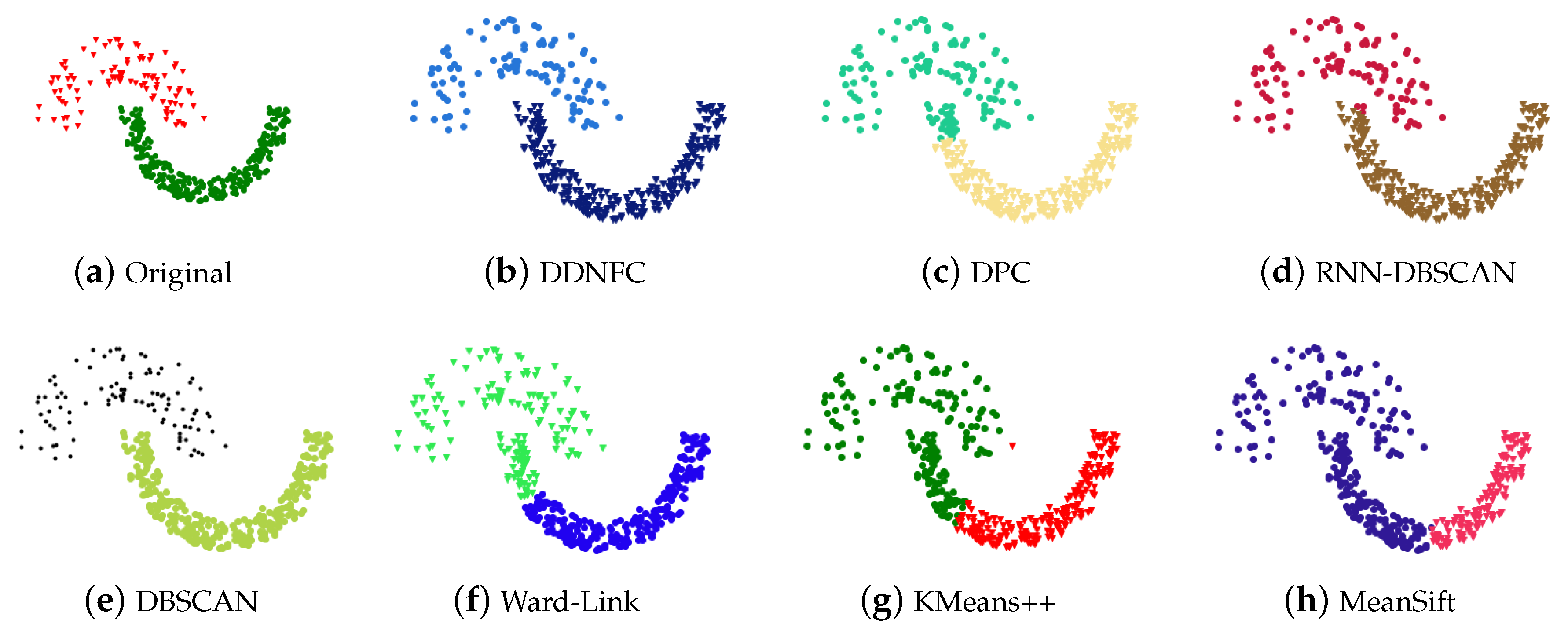
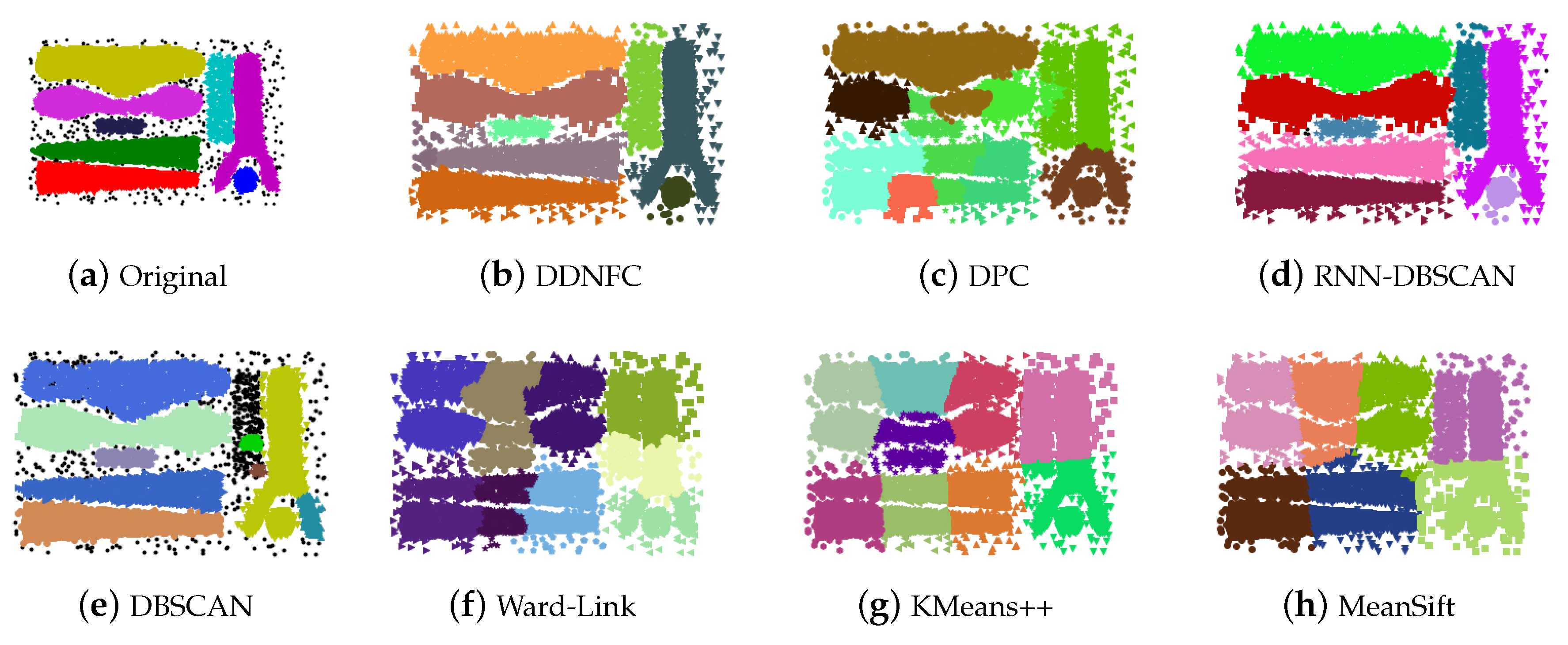
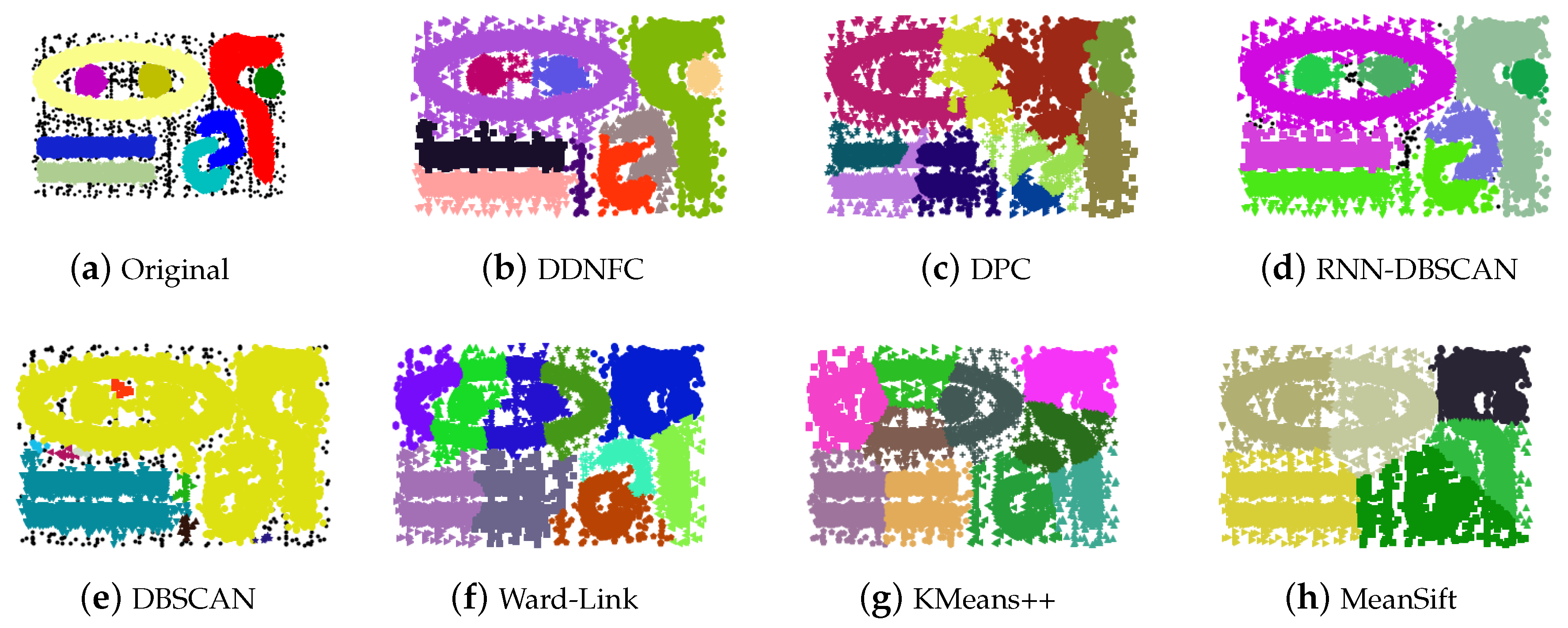
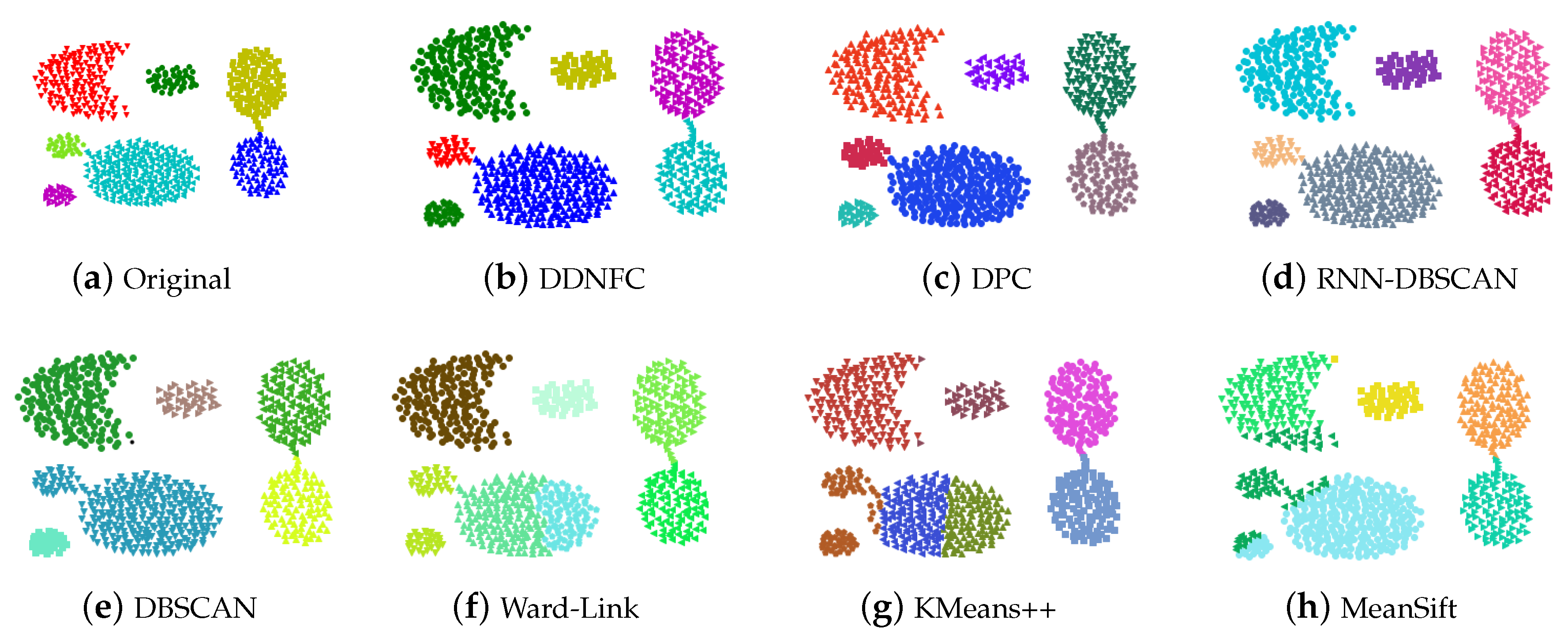
Meanwhile, we display some results of the above seven algorithms running on these data sets. Figure 3 and Figure 4 show the results of Compound and Pathbased, and other results are showed in Appendix A Figure A1, Figure A2, Figure A3, Figure A4 and Figure A5. Different clusters are distinguished by marks with different shapes and colors. Small black dots represent unrecognized data, i.e., noise points.

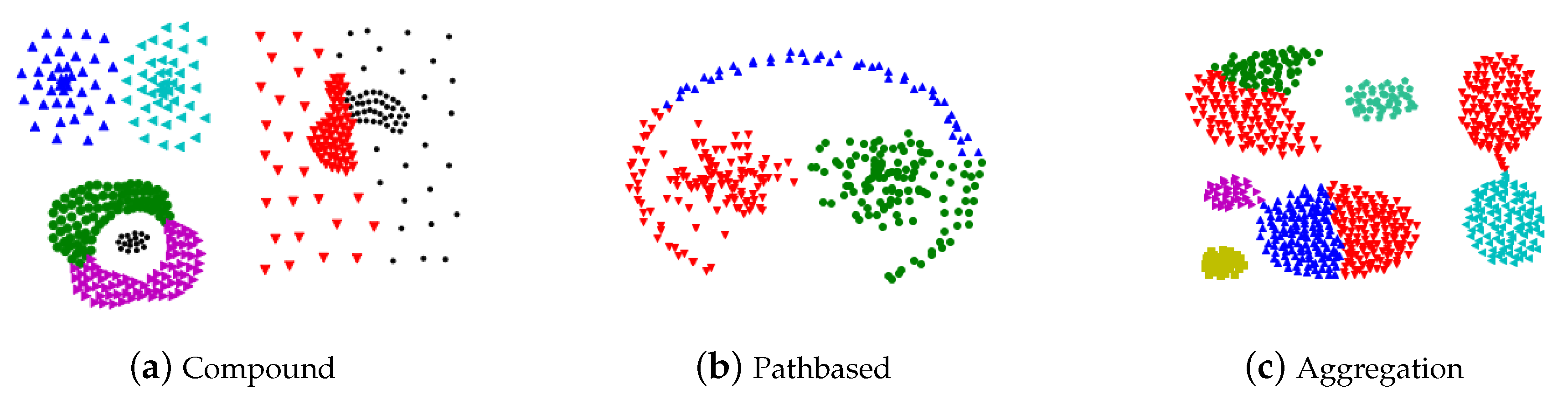
Compound is composed of six classes with different densities. In the upper-left corner, two classes are adjacent to each other and both subject to Gaussian distribution. In the right side area, an irregular shape class is surrounded by a sparse distributed class and the two classes are overlap spatially. In the bottom-left corner, a small disk like class is encompassed by a ring-shape class. It is a big challenge to distinguish all classes correctly in Compound because they have different densities, various shapes and complex spatial relationships. As in Figure 3, our method classified all points correctly except one point on the border between two classes in the upper-left corner. RNN-DBSCAN also found six clusters, but nearly 75 percent points of the sparse class on the right side are misclassified to the dense cluster. DBSCAN only detected out five clusters, and a large number of points are divided into noise as the sixth cluster of data set. DPC almost distinguished the two Gaussian and the disk classes correctly, but partitioned the ring class into two parts and mingled the sparse class with the dense. The results of Ward-Link and K-Means++ showed that the two methods are unable to cluster arbitrary shape data set. Meanshift cannot partition two clusters when one contains another, so it only recognized four clusters in Compound.

Pathbased has 3 classes, in which one contains 110 points form an unclosed thin ring, the other two contain 97 points and 93 points separately and all are enclosed in the ring. It is easy to misclassify the points, which belong to the ring class but are near other classes, to their adjacent class. As shown in Figure 4, DDNFS and RNN-DBSCAN get the nearly correct results, a few points in the adjacent space between the ring and the left class were misclassified. One point is not unrecognized by RNN-DBSCAN. DBSCAN found out two clusters but were treat points of the ring class as noise. The other four algorithms divided the ring clusters into three parts, the top of the arc area was regarded as a class, and the other two parts were respectively were clustered into the other two clusters.

Jain is composed of two lunate clusters with different densities. The upper left one is sparse and unevenly distributed. The other is dense and long. DDNFC partitioned the two classes completely correct. DBSCAN regarded the lower density class as noise again. The others have different degrees of misclassification.

Flame has two classes with similar densities but different shapes, and they are very close to each other. As the results shown in Figure A2 and Table 2, the algorithms based on density can find out two clusters more accurately, except for some classification errors in the adjacent parts between the two clusters. DDNFC got the completely correct result; DBSCAN treated two outliers in the upper left corner as noise. Obviously, in this data set, the algorithm based on density is obviously superior to the other three clustering algorithms.

The characteristics of t8.8k and t7.10k are similar to Compound, in which the clusters have different shapes and some are embraced or semi-embraced by others. But the two data sets are seriously contaminated by noise. On these two data sets, DDNFC and RNN-DBSCAN got more accurate clustering results than the other methods.

Seven clusters with different sizes in Aggregation are independent of each other, except two pairs are connected slightly. Four density-based methods achieved better results than the others. DDFNC misclassified three points located in the adjacent area between the right two clusters. RNN-DBSCAN misclassified one point located in the adjacent area between the left two connected clusters. DBSCAN regarded one edge point of the upper-left cluster as noise. DPC performed best in this data set.

In addition to the above 7 data sets, Table 2 also lists the test result of the 7 algorithms on the other 5 data sets.

The data sets t5.8k contain 7 clusters, 6 of which form the word “GEORGE”, and another bar-shape cluster runs through them. The data set contain noise data. As shown in Table 2, the results of all methods are not good because the bar-shape cluster is hard to recognize from the data set.

Clusters in the data sets Unbalance, R15, S1 and A3 are in general independent to each other, though some of them may be adjacent. Of course, the clusters have different densities and arbitrary shapes. On these data sets, DDNFC performed as well as the other algorithms.

The spectral clustering algorithm in scikit-learn library [24] need two parameters: the number of clusters and the number of nearest neighbors.

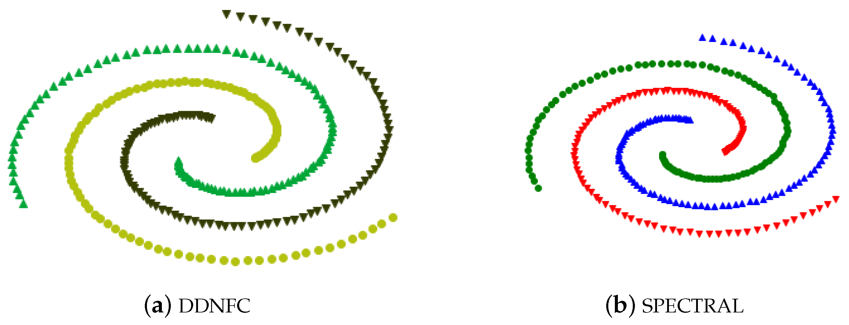
On Spiral, the k of DDNFC was set to 4, and the two parameters of spectral clustering were 3 and 4 respectively, and the results shown in Figure 5 are all entirely correct.

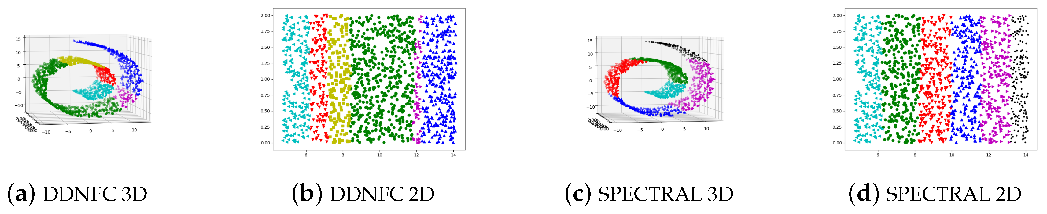
The Swissroll has 1500 points. The parameter settings of the two methods were 13 for DDNFC and (6, 13) for spectral clustering. From Figure 6 we can see that the width of clusters got by spectral clustering are more uniform than DDNFC.

On remain three data sets Compound, Pathbased, and Aggregation, the parameter settings of the spectral clustering were (6, 5), (3, 6), and (7, 9). As shown in Figure A6, the algorithm cannot classify the clusters in these data sets correctly.

4.2. Experiments on Real-World Data Sets and Results Analysis

Table 3. Real-world data sets.

Data Set	Size	Dimension	Cluster Number
Ionosphere	351	34	2
Page-blocks	5437	10	5
Haberman	306	3	2
SPECT-train	80	22	2
Segmentation	2100	19	7
Chess	3196	36	2
Breast-cancer-Wisconsin	699	10	2
Pendigits-train	7494	16	10
Sonar	208	60	2
Echocardiogram	106	7	2
Contraceptive-Method-Choice	1473	9	3
Wilt-train	4339	5	2

lists 12 real-world data sets, which are widely used in clustering and classification methods testing and downloaded from UCI machine learning repository [27] for testing the algorithms in this paper.

Additionally, we did data preprocessing on the data sets if needed.

• Data that have null values, uncertain values, or duplicates were removed.
• Most of data sets have a class attribute. Table 3 only gives the number of none class attributes.
• We conserved from the third to ninth features of the data in Echocardiogram because some of its data has missing values.

As shown in Table 3, Ionosphere, SPECT-train and Sona are sparse data sets for their higher ratio of dimension and number of instances. Ionosphere has 351 radar data. Each data is composed of 17 pulse numbers which are described by 2 attributes each, corresponding to the complex values. But in our tests, we treated 34 attributes as being independent. SPECT-train is one of a subset of SPECT, which has 22 binary attributes and 2 groups with 40 points each. Sona has 208 data with 60 real features. From

Table 4. Experiment results on real-world data sets.

Algorithm	Par	c/C	F1	AMI	ARI		Par	c/C	F1	AMI	ARI
	Ionosphere						Page-blocks
DDNFC	22	2/2	0.89	0.47	0.60		25	5/5	0.90	0.26	0.45
DPC	4.5	2/2	0.79	0.22	0.32		1.5	5/5	0.86	0.04	0.10
RNN-DBSCAN	6	2/2	0.69	0.01	0.01		19	5/5	0.90	0.26	0.48
DBSCAN	0.45/8	2/2	0.65	0.09	−0.05		0.1/5	7/5	0.86	0.04	0.07
Ward-Link	2	2/2	0.72	0.13	0.19		3	5/5	0.80	0.05	0.02
K-Means++	2	2/2	0.72	0.13	0.18		5	5/5	0.82	0.05	0.02
MeanShift	-	1/2	-	-	-		-	1/5	-	-	-
	Haberman						SPECT-train
DDNFC	10	2/2	0.73	0.01	0.05		4	2/2	0.70	0.14	0.21
DPC	1.5	2/2	0.61	−0.00	0.01		1.0	2/2	0.66	−0.01	−0.00
RNN-DBSCAN	10	2/2	0.73	−0.00	0.01		19	2/2	0.64	0.10	0.04
DBSCAN	0.1/5	1/2	-	-	-		0.1/5	2/2	0.62	0.08	0.06
Ward-Link	2	2/2	0.61	0.00	−0.02		2	2/2	0.61	0.03	0.04
K-Means++	2	2/2	0.55	−0.00	−0.00		2	2/2	0.70	0.17	0.17
MeanShift	-	2/2	0.73	−0.00	0.01		-	1/2	-	-	-
	Segmentation						Chess
DDNFC	17	7/7	0.67	0.59	0.42		15	2/2	0.67	0.00	0.00
DPC	1.0	7/7	0.57	0.52	0.35		2.0	2/2	0.61	0.00	0.01
RNN-DBSCAN	13	6/7	0.60	0.56	0.38		9	2/2	0.67	0.00	0.00
DBSCAN	0.1/5	1/7	-	-	-		0.1/5	1/2	-	-	-
Ward-Link	7	7/7	0.57	0.46	0.32		2	2/2	0.59	0.01	0.00
K-Means++	7	7/7	0.54	0.48	0.33		2	2/2	0.51	0.00	0.00
MeanShift	-	7/7	0.38	0.20	0.10		-	1/2	-	-	-
	Breast-cancer-Wisconsin						Pendigits-train
DDNFC	27	2/2	0.94	0.65	0.77		60	10/10	0.73	0.70	0.55
DPC	3.0	2/2	0.59	0.20	0.02		1.0	10/10	0.73	0.73	0.61
RNN-DBSCAN	39	2/2	0.69	0.00	0.00		32	10/10	0.68	0.63	0.41
DBSCAN	0.1/26	2/2	0.68	0.03	−0.03		0.1/5	1/10	-	-	-
Ward-Link	2	2/2	0.97	0.79	0.87		10	10/10	0.75	0.72	0.59
K-Means++	2	2/2	0.96	0.74	0.85		10	10/10	0.71	0.67	0.54
MeanShift	-	4/2	0.95	0.68	0.84		-	3/10	0.34	0.23	0.17
	Sonar						Echocardiogram
DDNFC	11	2/2	0.66	0.02	0.01		7	2/2	0.71	0.03	0.05
DPC	1.0	2/2	0.57	−0.00	−0.00		1.0	2/2	0.70	0.01	0.06
RNN-DBSCAN	7	2/2	0.67	−0.00	−0.00		4	2/2	0.70	−0.00	0.04
DBSCAN	0.35/5	3/2	0.65	0.05	−0.01		0.1/5	1/2	-	-	-
Ward-Link	2	2/2	0.58	−0.00	−0.00		2	2/2	0.72	0.10	0.16
K-Means++	2	2/2	0.54	0.00	0.00		2	2/2	0.73	0.11	0.19
MeanShift	-	-	-	-	-		-	2/2	0.71	0.00	0.04
	Contraceptive-Method-Choice						Wilt-train
DDNFC	9	3/3	0.52	0.00	−0.00		12	2/2	0.68	0.00	-0.00
DPC	1.0	3/3	0.43	0.02	0.02		1.0	2/2	0.68	−0.00	−0.00
RNN-DBSCAN	19	2/3	0.52	−0.00	−0.00		29	2/2	0.68	−0.00	−0.00
DBSCAN	0.1/5	1/3	-	-	-		0.1/5	1/2	-	-	-
Ward-Link	3	3/3	0.39	0.03	0.02		2	2/2	0.55	0.01	-0.00
K-Means++	3	3/3	0.41	0.03	0.03		2	2/2	0.55	0.00	0.00
MeanShift	-	2/3	0.46	0.01	0.01		-	3/2	0.68	0.01	−0.01

Note: The bold numbers in the table indicate the best results the algorithm obtained. The underline numbers mean the algorithm got uncorrect number of clusters. If the algorithm failed to classify a data set, the corresponding lines of results were set to ‘-’.

, we can see that DDNFC outperformed other six algorithms on all benchmarks much more on Ionosphere and also got the best results on two benchmarks on SPECT-train and Sona. The three data sets are sparse, DPC was better than the other 5 methods. Meanshift cannot distinguish the data in these data sets. KMeans++ performed good on SPECT-train. RNN-DBSCAN got the highest F1 on Sona.

Page-block is a data set about classification of the blocks of the page layout in a document. Its data has 4 real-type and 6 integer-type features. It has 5 classes with 4913, 329, 28, 88 and 115 data, respectively. Haberman contains 306 cases of the survival status of patients with breast cancers after they had undergone surgery. The 3 attributes of each data are integers representing operating time, patient’s year and number of positive axillary nodes detected. The data set is divided into 2 groups with 225 and 81 instances, respectively. Wilt-train consists two groups, one group has 4265 points but another has only 74 points. Obviously, the three data sets are unbalance data sets. The test results on them show that density-based clustering methods were better than others. DDNFC and RNN-DBSCAN got the best results. The two methods performed closely because they all used reverse k nearest neighbors model to determine core objects and the nearest-on-first-in tragedy of our method was not different from RNN-DBSCAN on these unbalance data sets. DBSCAN method performed badly.

The attributes of data in Breast-cancer-Wisconsin are integer category type. The original data set has 458 benign and 241 malignant cases, but we deleted cases with missing values. There are 444 benign and 239 malignant cases remained. Each data of Chess has 36 text category type attributes. The value of each attribute are selected from one of four groups f, t, g, l, b, n, w and n, t. For calculating the distance between two data, we replace the text label values of data to integer such as 0, 1, 2. The attributes of Breast-cancer-Wisconsin, Chess and Pendigits-train are categories or integers. On Breast-cancer-Wisconsin, Ward-link, KMeans++ and DDNFC got much higher benchmarks than the other methods, and DDNFC got the best performance in the density-based methods. On other two data sets, the performances of DDNFC, Ward-link, DPC and RNN-DBSCAN were close.

Table 4 shows the settings of parameters (dubbed as par) and the test results, such as the number of clusters the methods obtain and the true cluster numbers (dubbed as c/C), the values of F1, AMI and ARI, of the above seven algorithms on artificial and real data sets respectively.

Contraceptive-Method-Choice is a subset of the National Indonesia Contraceptive Prevalence Survey in 1987, which has multi-type attributes including integer, category and binary. The attributes of Echocardiogram are also composed of different numeric types with different value scales. On Echocardiogram, all methods except DBSCAN got the similar results. KMeans++ was the best one in all while DDNFC was the best one in density-based methods. On Contraceptive-Method-Choice, only four methods got the correct number of clusters. DDNFC achieved the best F1.

Segmentation-test is one of a subset of Segmentation, which has 19 real attributes, 7 groups with 300 points each. It is an ordinary data set. RNN-DBSCAN and DBSCAN did not classify all 7 clusters. DDNFC outperformed all.

5. Conclusions

In this paper, in order to deal with data sets with mixed density clusters, we proposed a density clustering method, DDNFC, based on the strategy of double density and Nearest-to-First-in. DDNFC uses two density calculation methods to estimate the data distributions in a data set. By thresholding on the data set with two densities respectively, DDNFC can more accurately partition the data into high-density core area and low-density boundary area initially. In the process of classification of low density points, the sensitivity of the clustering to the input parameters and the data storage order is reduced by applying the Nearest-to-First-in strategy. By comparing the proposed algorithm in this paper and other classical algorithms on artificial and real data sets, the results show that DDNFC is better than the other six algorithms as a whole.

References

- Aggarwal, C.C.; Reddy, C.K. Data Clustering Algorithms and Applications, 1st ed.; CRC Press: Boca Raton, FL, USA, 2013; pp. 65–210. [Google Scholar]
- Arthur, D.; Vassilvitskii, S. K-means++: The advantages of careful seeding. In Proceedings of the Annual ACM-SIAM Symposium on Discrete Algorithms, New Orleans, LA, USA, 7–9 January 2007; pp. 1027–1035. [Google Scholar]
- Murtagh, F.; Legendre, P. Ward’s Hierarchical Agglomerative Clustering Method: Which Algorithms Implement Ward’s Criterion? J. Classif. 2014, 31, 274–295. [Google Scholar] [CrossRef] [Green Version]
- Wu, K.L.; Yang, M.S. Mean shift-based clustering. Pattern Recognit. 2007, 40, 3035–3052. [Google Scholar] [CrossRef]
- Jiang, Z.; Liu, X.; Sun, M. A Density Peak Clustering Algorithm Based on the K-Nearest Shannon Entropy and Tissue-Like P System. Math. Probl. Eng. 2019, 2019, 1–13. [Google Scholar] [CrossRef] [Green Version]
- Halim, Z.; Khattak, J.H. Density-based clustering of big probabilistic graphs. Evol. Syst. 2019, 10, 333–350. [Google Scholar] [CrossRef]
- Wu, C.; Lee, J.; Isokawa, T.; Yao, J.; Xia, Y. Efficient Clustering Method Based on Density Peaks with Symmetric Neighborhood Relationship. IEEE Access 2019, 7, 60684–60696. [Google Scholar] [CrossRef]
- Tan, H.; Gao, Y.; Ma, Z. Regularized constraint subspace based method for image set classification. Pattern Recognit. 2018, 76, 434–448. [Google Scholar] [CrossRef]
- Chen, Y.; Tang, S.; Zhou, L.; Wang, C.; Du, J.; Wang, T.; Pei, S. Decentralized Clustering by Finding Loose and Distributed Density Cores. Inf. Sci. 2018, 433, 510–526. [Google Scholar] [CrossRef]
- Wang, Z.; Yu, Z.; Philip Chen, C.L.; You, J.; Gu, T.; Wong, H.S.; Zhang, J. Clustering by Local Gravitation. IEEE Trans. Cybern. 2018, 48, 1383–1396. [Google Scholar] [CrossRef]
- Oktar, Y.; Turkan, M. A review of sparsity-based clustering methods. Signal Process. 2018, 148, 20–30. [Google Scholar] [CrossRef]
- Chen, J.; Zheng, H.; Lin, X.; Wu, Y.; Su, M. A novel image segmentation method based on fast density clustering algorithm. Eng. Appl. Artif. Intell. 2018, 73, 92–110. [Google Scholar] [CrossRef]
- Zhou, R.; Zhang, Y.; Feng, S.; Luktarhan, N. A novel hierarchical clustering algorithm based on density peaks for complex datasets. Complexity 2018, 2018, 1–8. [Google Scholar] [CrossRef]
- Zhang, X.; Liu, H.; Zhang, X. Novel density-based and hierarchical density-based clustering algorithms for uncertain data. Neural Netw. 2017, 93, 240–255. [Google Scholar] [CrossRef] [PubMed]
- Wu, B.; Wilamowski, B.M. A fast density and grid based clustering method for data with arbitrary shapes and noise. IEEE Trans. Ind. Inform. 2017, 13, 1620–1628. [Google Scholar] [CrossRef]
- Lv, Y.; Ma, T.; Tang, M.; Cao, J.; Tian, Y.; Al-Dhelaan, A.; Al-Rodhaan, M. An efficient and scalable density-based clustering algorithm for datasets with complex structures. Neurocomputing 2016, 171, 9–22. [Google Scholar] [CrossRef]
- Ester, M.; Kriegel, H.P.; Sander, J.; Xu, X. A Density-Based Algorithm for Discovering Clusters in Large Spatial Databases with Noise. In Proceedings of the 2nd International Conference on Knowledge Discovery and Data Mining, Portland, OR, USA, 2–4 August 1996; pp. 226–231. [Google Scholar]
- Rodriguez, A.; Laio, A. Clustering by fast search and find of density peaks. Science 2014, 344, 1492–1496. [Google Scholar] [CrossRef] [PubMed] [Green Version]
- Vadapalli, S.; Valluri, S.R.; Karlapalem, K. A simple yet effective data clustering algorithm. In Proceedings of the IEEE International Conference on Data Mining, Hong Kong, China, 18–22 December 2006; pp. 1108–1112. [Google Scholar] [CrossRef]
- Fränti, P.; Sieranoja, S. K-means properties on six clustering benchmark datasets. Appl. Intell. 2018, 48, 4743–4759. [Google Scholar] [CrossRef]
- Bryant, A.; Cios, K. RNN-DBSCAN: A density-based clustering algorithm using reverse nearest neighbor density estimates. IEEE Trans. Knowl. Data Eng. 2018, 30, 1109–1121. [Google Scholar] [CrossRef]
- Romano, S.; Vinh, N.X.; Bailey, J.; Verspoor, K. Adjusting for chance clustering comparison measures. J. Mach. Learn. Res. 2016, 17, 1–32. [Google Scholar]
- Xie, J.; Xiong, Z.Y.; Dai, Q.Z.; Wang, X.X.; Zhang, Y.F. A new internal index based on density core for clustering validation. Inf. Sci. 2020, 506, 346–365. [Google Scholar] [CrossRef]
- Pedregosa, F.; Varoquaux, G.; Gramfort, A.; Michel, V.; Thirion, B.; Grisel, O.; Blondel, M.; Prettenhofer, P.; Weiss, R.; Dubourg, V.; et al. Scikit-learn: Machine Learning in Python. J. Mach. Learn. Res. 2011, 12, 2825–2830. [Google Scholar]
- Von Luxburg, U. A tutorial on spectral clustering. Stat. Comput. 2007, 17, 395–416. [Google Scholar] [CrossRef]
- Karypis, G.; Han, E.H.; Kumar, V. Chameleon: Hierarchical clustering using dynamic modeling. Computer 1999, 32, 68–75. [Google Scholar] [CrossRef] [Green Version]
- Dua, D.; Graff, C. UCI Machine Learning Repository. Available online: https://archive.ics.uci.edu/ml/index.php (accessed on 1 October 2017).
Figure 1.
Compound data set and the offset of local position of its point.
Figure 2.
Result of Algorithm 1. Initial clustering.
Figure 3.
Experiment results on Compound data set.
Figure 4.
Experiment results on Pathbased data set.
Figure 5.
Experiment results on Spiral data set.
Figure 6.
Experiment results on Swissroll data set.