Modified Integral Control Globally Counters Symmetry-Breaking Biases

Abstract

We propose a modified integral controller to treat actuation biases in nonholonomic systems. In such systems, although one cannot directly counter biases along all directions, one can still aim at restoring the symmetry of coordinated motion that the biases would break. Focusing on the example of steering controlled planar vehicles, we indeed show how to perfectly stabilize a circular trajectory coordinated with the leader, despite any unknown actuation bias. The proposed solution is a simple modified integral control term, and we prove via a detailed analysis of averaging theory that this control gadget globally stabilizes the perfect coordinated motion. The corresponding general observation is that stabilizing such symmetry-preserving situation can be viewed as rejecting a bias affecting the output measurement, instead of the input command. The symmetry-restoring control then becomes an output bias rejection, dual to the more standard input bias rejection with standard integral control.

1. Introduction

Coordinated motion of controlled vehicles in robotics has drawn great attention during the last two decades [1,2,3,4,5]. A basic control primitive is to design local interactions among vehicles, such that their emerging behavior corresponds to moving like a single rigid body. This stabilizes a manifold of states corresponding to the symmetry of invariant relative configuration, and leaves open how one might further drive the swarm along this manifold, towards specific relative configurations or a specific motion of the center of mass [3,5]. The most notable examples are steering-controlled vehicles (see same references). Control laws and performance proofs have been established, assuming that all the vehicles have exactly equal dynamics. However, real vehicles will not satisfy this symmetry under permutation perfectly. Part of this modeling error will be countered purposefully by the coordination controller, avoiding vehicles to drift completely apart over long times. However, small modeling errors that break the permutation symmetry will typically, also in the presence of control, break the target symmetry of coordinated motion: due to small residual velocity errors, vehicles will slowly but persistently drift with respect to each other (see simulations in Section 4 for an illustration). Depending on the application context, such unexpected symmetry breaking could be truly detrimental and it appears meaningful to search for a simple fix of the situation. The improved controller might also serve in other applications like information protection codes, where the very purpose is to isolate thanks to coordination mechanisms, a symmetric manifold on which realistic perturbations imply a minimal drift.

When a system is subject to time-independent biases, a control engineering standard is to write a dynamical observer algorithm, which estimates the values of the bias parameters from all the known signals—i.e., input commands and output measurements. A well-designed estimator should asymptotically converge towards the true bias values, and those can then be explicitly compensated for in the input commands. The canonical way of writing such an estimator builds on Bayes reasoning, using a full copy, inside the algorithm, of the system to be controlled. However, relying on the stabilization provided by feedback control, less accurate and much simpler bias-compensating schemes are also viable. One such approach, which we pursue in the present paper, is integral control [6]. This concept just adds to the control input, a term proportional to the integral of the measured error. Under a constant nonzero error, the integral would keep increasing, so if the system stabilizes to a constant value, this must correspond to zero error. A system analysis is then needed to prove that the system indeed converges, but usually this can be established under quite general properties without requiring detailed system knowledge.

The idea in the present paper is thus to apply this integral control strategy in order to restore perfect symmetry in coordinated motion, despite possible biases that make the subsystems different from each other. This application features two particular challenges:

• The state space and therefore the error space is not a linear vector space, but a nonlinear manifold, more precisely a compact Lie group. This requires to revisit the concept of “integrating the error”, since summing up or integrating variables relies on a vector space structure. The solution in [7,8] proposes to integrate instead the error-proportional feedback action, brought back to the Lie algebra (which is a vector space) thanks to standard Lie group operations. This error-proportional feedback is the main controller in standard studies without bias, like [1,4,5], and we thus only suggest to add a small multiple of its integral. The idea is that, similarly, if an error-proportional feedback action constantly fights against the same bias, then the integral would keep increasing; so if the controlled system stabilizes it must be at a situation with zero error-proportional feedback action, hence in principle (under some conditions, and at least locally) with zero error. By assuming full actuation, Refs. [7,8] prove that any constant bias on a Lie group can be countered in this way.
• A new challenge in the present paper is the nonholonomic actuation typical of such systems, also sometimes called underactuation. This means that, if a bias pushes the system with some vector v, it is not necessarily physically possible with our actuator to push in the direction $-v$ even if we knew it. Think for instance of a ship subject to lateral drift, or of a steering-controlled vehicle with translation velocity fixed at a wrong value. In standard linear control, this situation can appear as well. Consider $\dot{x}=Ax+Bu+Fv$ with perturbation force $Fv$ that lies outside the range of actuation $Bu$; then, there is no way to stabilize $x=0$ exactly, since this simply cannot be made a steady state. In the coordination application, the goal is to stabilize a manifold of relative equilibria corresponding to any configuration compatible with synchronized right-invariant Lie group velocities [9,10]. Configurations where the vehicles can keep moving in a coordinated way appear feasible even for nonholonomic systems with uncountered bias.

We here propose a simple modified integral control gadget, which we call moderating integral control (MIC) as it acts by reducing the error-proportional output feedback in a suitable way, and which indeed stabilizes coordinated motion perfectly, despite actuation biases and for underactuated systems. In the present paper, we develop this idea in detail for steering controlled planar vehicles. We prove that our MIC not only restores symmetry exactly, but it ensures global convergence to this situation from any initial condition, like in the absence of bias the original error-proportional feedback controller did. It thus appears like a plug-and-play adaptation which could open up discussion for a more general use of integral control as a mechanism in symmetry-restoring applications.

As an independent observation, we note that the MIC is a suitable algorithm integrating accurate inputs to reject bias in outputs; this is dual to the usual integral control integrating accurate outputs to reject bias in inputs.

The paper is organized as follows:

• In Section 2, we describe the abstract Lie group model for stabilizing an underactuated rigid body in a fixed relative configuration with respect to a swarm leader, which is thus the geometric invariant related to the symmetry of rigid body motions. While Refs. [4,5,10], among others, have derived corresponding controllers for perfectly modeled vehicles, we insist on achieving the same performance when the controlled vehicle is subject to biases or calibration errors on its translation velocity, both on actuated and on unactuated directions of motion. We progressively explain why coordinated motion/restoring symmetry is a proper objective in the presence of bias. We end this section by proposing a moderating integral controller (MIC) to solve this task.
• In Section 3, we carry out a detailed convergence analysis for stabilizing the steering controlled vehicle into a given circular motion ([4], see [3] for a concrete application), despite the actuation biases. We start the section by a more concrete formulation for the steering controlled vehicle in the plane. The main result proves how our MIC allows for still ensuring global convergence towards exact coordinated motion. The result combines a Lyapunov function adapted from the bias-less case [5,10], with a detailed analysis of averaging theory along the lines of [11], and showing that the averaging approximation becomes exact as we approach the target.
• Section 4 provides simulation results illustrating the working of our controller for the steering controlled vehicle and giving a hint at expected performance.
• In Section 5, we note how the MIC can be reformulated in an abstract context of output biases, to possibly solve problems beyond symmetry-preservation. In particular, we discuss its application to linear systems, where it enables a trade-off between rejecting biases on the input or on the output.

2. General Problem Setting and Controller Definition

2.1. Underactuated Rigid Body Motion

The motion of a rigid body can be described on a Lie group by

$$\frac{d}{dt}g=g\xi ,$$

where g is the position on the Lie group $\mathcal{G}$ and $\xi$ is the Lie velocity in body frame; the latter belongs to the Lie algebra $\mathfrak{g}$, i.e., the tangent vector space to the Lie group at identity. Examples of this model include rigid body attitude control, where g is a rotation matrix and $\xi$ is an angular velocity matrix [2]; or the motion of a steering controlled vehicle [4], where

$$g=\left(\begin{array}{ccc}cos\theta & sin\theta & p_x\\ -sin\theta & cos\theta & p_y\\ 0& 0& 1\end{array}\right),\xi =\left(\begin{array}{ccc}0& \omega & v\\ -\omega & 0& 0\\ 0& 0& 0\end{array}\right),$$

(1)

with $p_x,p_y$ the vehicle position, $\theta$ its heading, v a fixed translation velocity in body frame and $\omega$ the controlled angular rotation rate. We will treat this last example concretely and in detail.

For controlling satellite orientation, one can usually apply any angular velocity in $\mathfrak{g}=\mathfrak{so}\left(3\right)(fullactuation$ [2]). In contrast, a vehicle can usually not have a sidewards velocity; in model (1), we can command one single degree of freedom in $\xi$, which is thus restricted to a subset of $\mathfrak{g}=\mathfrak{se}\left(2\right)$. This situation is called underactuation or nonholonomic motion. While a nonholonomic system may still reach all $g\in \mathcal{G}$, i.e., for the vehicle all the three-dimensional values of heading $\theta$ and position $p_x,p_y$, it can only do so indirectly, and this complicates bias rejection.

Nonholonomic systems are standard in geometric control and the stabilization of symmetries (see the next paragraph). However, surprisingly little has been said about what happens to symmetries when the actual vehicle model differs from the nominal one. We therefore introduce an actuation bias explicitly into the model:

$$\xi =A+u+u_B,$$

where $A\in \mathfrak{g}$ is a fixed drift velocity, the control u belongs to a subspace $\mathcal{U}\subset \mathfrak{g}$ orthogonal to A, and $u_B\in \mathfrak{g}$ is an actuation bias.

When $u_B$ lies in the same subspace $\mathcal{U}$ as u, countering the bias comes down to knowing its value and applying an opposite correction, $u=-u_B+u_0$ where $u_0\in \mathcal{U}$ would be the control input applied in the absence of bias. One approach is to write a so-called dynamical observer [12,13,14,15], which estimates all the variables that have known dynamical models, including the constant biases. A computationally less intensive approach would use integral control [6]. If the nominal input is $u=u_0$ and the measured deviation from target at time t is $e\left(t\right)$, then standard integral control applies $u=u_0-k_I{u}_I$ with

$$\frac{d}{dt}{u}_I\left(t\right)=e\left(t\right).$$

(2)

Thus, “the longer the error has been positive, the stronger we consider pushing in the negative direction”. Mathematically, if $u_I$ stabilizes to a fixed value, then Equation (2) implies $e\left(t\right)=0$. The computation (2) only makes sense if $u_I$ and e belong to the same vector space. Thus, if for instance $u_I$ is a Lie group velocity and e a Lie group configuration (error) as in (1), it must be adapted. In [7,8] concurrently, it has been proposed how to adapt (2) for Lie groups where $\mathcal{U}=\mathfrak{g}$, i.e., under full actuation. Indeed, since $u_0$ is usually reflecting how much we push against the configuration error, it is proposed to replace (2) by

$$\frac{d}{dt}{u}_I\left(t\right)=-u_0\left(t\right).$$

(3)

Thus, “the longer we have been pushing in the negative direction, the stronger we consider pushing in that direction”. The equation always makes sense since both $u_0$ and $u_I$ belong to $\mathfrak{g}$, e.g., for rigid body motion they represent the rotational velocity and translation velocity expressed in body frame. It is proven that, for appropriate tuning, a first-order or second-order integrator on a Lie group can be stabilized towards $u_0=0$ and $u_I+u_B=0$ with this approach.

The present paper addresses the case where $u_B\notin \mathcal{U}$, such that it is not possible to just cancel it with the control input. For instance in steering control, if the translation velocity v differs from its nominal value, then this cannot be directly canceled by changing the value of our control input $\omega$ (rotation rate). In this case, we must find an objective that is compatible with the presence of $u_B$; this brings us to coordinated motion.

2.2. Coordinated Motion

For the case with $u_B=0$, we follow the framework of [10], which was developed as a general theory behind proposals like [4,5] for steering control in the plane.

A set of rigid bodies is said to undergo a coordinated motion if their configuration at any time t is equal to their configuration at time 0, up to a symmetry transformation of the reference frame. In other words, the whole set moves together like a single rigid body. Ensuring coordinated motion can be seen as imposing symmetry on the behavior of the set of vehicles.

In the Lie group notation, coordinated motion of a vehicle $g\left(t\right)$ with respect to a reference vehicle $g_{\mathrm{ref}}\left(t\right)$ corresponds to keeping a fixed relative configuration

$$\frac{d}{dt}\left(g^{-1}{g}_{\mathrm{ref}}\right)=0.$$

In terms of velocities expressed in body frame, this is equivalent to

$$\xi ={\mathrm{Ad}}_{g^{-1}{g}_{\mathrm{ref}}}{\xi }_{\mathrm{ref}},$$

(4)

where ${\mathrm{Ad}}_h$ is the adjoint action of h on the Lie algebra; in terms of matrices, we have ${\xi }^{-1}=-\xi$ and ${\mathrm{Ad}}_h\left(\xi \right)=h\xi h^{-1}$. Note that this adjoint action is not just a rotation since h in general is not unitary: it really expresses which combination of translation and rotation velocities $\xi$, at a configuration g, would correspond to a coordinated motion with a vehicle applying ${\xi }_{\mathrm{ref}}$ at configuration $g_{\mathrm{ref}}$. Once (4) is achieved at a given time, keeping ${\xi }_{\mathrm{ref}}$ and $\xi$ fixed will ensure that it stays like this for all times, since by definition ${\mathrm{Ad}}_{g^{-1}{g}_{\mathrm{ref}}}$ also stays fixed. Such situations are known as relative equilibria and they form basic primitives for further control [9].

For instance, for planar vehicles, we can apply the above with matrix expressions (1). Consider at time t a reference configuration $g_{\mathrm{ref}}$ with ${(p_x,p_y,\theta )}_{\mathrm{ref}}=(1,0,\pi /2)$ and following a circular trajectory of radius 1 around the origin, by applying ${\xi }_{\mathrm{ref}}$ with $(\omega ,v)=(1,2\pi )$. Consider a tracking vehicle at configuration g with $(p_x,p_y,\theta )=(2,0,\pi /2)$. Intuitively, to maintain coordinated motion, i.e., reference and tracking vehicles moving together like a single rigid body, the tracking vehicle would have to follow a circle of twice the radius of the reference. Mathematically, using matrix expressions (1), the relative configuration $g^{-1}{g}_{\mathrm{ref}}$ corresponds to $\left(Q_{\theta }^{-1}\left((p_x,p_y)\mathrm{ref}-(p_x,p_y)\right),{\theta }_{\mathrm{ref}}-\theta \right)=(0,-1,0)$, where $Q_{\theta }$ is the $2\times 2$ rotation matrix by angle $\theta$ in the upper-left block of g. This $g^{-1}{g}_{\mathrm{ref}}$ expresses the relative position and orientation of the reference with respect to the tracking vehicle, in the reference frame attached to the tracking vehicle. Coordinated motion requires that this remains constant over time. The corresponding velocity that would achieve this for the tracking vehicle is computed by (4) with the matrix expression ${\mathrm{Ad}}_h\left(\xi \right)=h\xi h^{-1}$; it yields that $\xi ={\mathrm{Ad}}_{g^{-1}{g}_{\mathrm{ref}}}{\xi }_{\mathrm{ref}}$ corresponds to $(\omega ,v)=(1,4\pi )$. This is in agreement with motion on a circle of radius 2 around the origin. By computing the derivative of relative position and orientation in body frame, one can check that applying this velocity indeed implies $\frac{d}{dt}\left(g^{-1}{g}_{\mathrm{ref}}\right)=0$, i.e., the result is consistent.

The condition (4) for coordinated motion constrains g indirectly, in a combination with $\xi$. When $\xi$ can be freely chosen in $\mathfrak{g}$, any relative position $g^{-1}{g}_{\mathrm{ref}}$ is compatible with a relative equilibrium. However, for nonholonomic systems, where $\xi$ is restricted to $\mathcal{U}$, relative equilibria can restrict the set of relative configurations $g^{-1}{g}_{\mathrm{ref}}$, namely to the situations where ${\mathrm{Ad}}_{g^{-1}{g}_{\mathrm{ref}}}{\xi }_{\mathrm{ref}}$ belongs to $\mathcal{U}$ (or more loosely if ${\xi }_{\mathrm{ref}}$ can be adapted inside $\mathcal{U}$, where the intersection of $\mathcal{U}$ with ${\mathrm{Ad}}_{g^{-1}{g}_{\mathrm{ref}}}\mathcal{U}$ is nonempty). In the case of a steering controlled vehicle (1) with v fixed and equal for all vehicles, there are two types of relative equilibria: parallel straight motion (${\omega }_{\mathrm{ref}}=0$), where the underactuation restricts all the headings to be equal; and rotation on a common circle (${\omega }_{\mathrm{ref}}\ne 0$), where thus the underactuation restricts positions and headings to be properly aligned on that circle. Papers like [4,5] for planar vehicles, and [10] more generally, have proposed control laws $u=u_0(g^{-1}{g}_{\mathrm{ref}},{\xi }_{\mathrm{ref}})$ to stabilize such coordinated motion for perfectly calibrated systems.

Stabilizing the symmetric motion (4) thus leaves some freedom on the actual g and $\xi$. The freedom on g is most visible, namely for a given solution $(g,\xi )$ any alternative $(\tilde{g}=hg,\xi ),$ where h satisfies ${\mathrm{Ad}}_h\xi =\xi$ is also a solution. This symmetry allows for complementing the controller stabilizing the coordinated motion by a controller that would specify particular relative configurations h, according to some other application needs and criteria. In addition, it is possible to satisfy (4) with a different $\xi$ i.e., a different velocity applied in body frame. This would allow for satisfying coordinated motion even in the presence of biases, where $\xi =A+u+u_B$. The possibilities depend on the range of ${\mathrm{Ad}}_g\xi$ viewed as a function of g. For instance, when g represents an orientation (see satellite attitude control, [1,2]), ${\mathrm{Ad}}_g$ corresponds to an orthogonal matrix and it is thus necessary that the available u and bias include the possibility $\parallel \xi \parallel =\parallel {\xi }_{\mathrm{ref}}\parallel$. For steering control, we must again distinguish two cases: if ${\omega }_{\mathrm{ref}}=0$, then $\parallel A{d}_g{\xi }_{\mathrm{ref}}\parallel =\parallel v_{\mathrm{ref}}\parallel$ for all g; whereas, if ${\omega }_{\mathrm{ref}}\ne 0$, then the set $\{A{d}_g{\xi }_{\mathrm{ref}}:g\in G\}=\{\xi \in \mathfrak{g}:\omega ={\omega }_{\mathrm{ref}}\}$, i.e., as long as we apply the same angular velocity, and independently of the translation velocity, we can always find a configuration where coordinated motion is possible. In other words, $\{A{d}_g\xi :g\in G,\xi \in \mathcal{U}\}$ corresponds to all of $\mathfrak{g}$ except the measure-zero set where $\omega =0$ and the translation velocity would differ from the one implied by $A+u_B$, or, more concretely, the symmetry of coordinated motion can be restored, in principle, for any circular reference motion and any bias. The question is how to design a simple control algorithm that would stabilize this coordinated motion.

2.3. A “Moderating” Integral Controller (MIC)

In the absence of bias, designs $u=u_0(g^{-1}{g}_{\mathrm{ref}},{\xi }_{\mathrm{ref}})$ have thus been proposed in e.g., [4,5] to stabilize coordinate motion. To explain our bias-rejection idea, we split the input in two terms $u=u_s+u_m$. The part $u_s$ corresponds to the steady-state motion once coordination is reached, i.e., there exists some $\tilde{h}$ such that

$$A{d}_{\tilde{h}}(A+u_s+u_B)={\xi }_{\mathrm{ref}},$$

(5)

and thus once this situation is reached it suffices to apply $u=u_s$ to have a coordinated motion. For the steering controlled vehicle, $u_s$ corresponds to ${\omega }_s={\omega }_{\mathrm{ref}}$. The part $u_m$ in contrast steers the system towards a relative configuration h satisfying (5). We denote by $u_P(g^{-1}{g}_{\mathrm{ref}},{\xi }_{\mathrm{ref}})=u_0-u_s$ the corresponding part of the controllers proposed in [4,5]. In the absence of bias, $u_m=u_P$ ensures that the vehicles asymptotically reach a coordinated motion, and so we also have $u_m=0$ asymptotically. In the presence of bias, our idea for restoring perfect symmetry is to add into the controller a term that explicitly targets $u_m=0$ asymptotically.

More precisely, in the presence of a bias, $u_P(g^{-1}{g}_{\mathrm{ref}},{\xi }_{\mathrm{ref}})=0$ will hold at configurations which do not correspond to a true coordinated motion; the configuration will thus change over time and, likely, $u_P$ will not remain zero. However, as $u_P$ does take a particular value $u_P\left(\tilde{h}\right)$ at each point $\tilde{h}$ which truly corresponds to a coordinated motion in the presence of bias, we can consider this value as a cancelable input bias and write an integral controller to cancel it:

$$\begin{array}{ccc}\hfill u_m& =& u_P\left(g^{-1}{g}_{\mathrm{ref}}\right)-k_I{u}_I\hfill \\ \hfill & =& u_P\left(\tilde{h}\right)+(u_P\left(g^{-1}{g}_{\mathrm{ref}}\right)-u_P\left(\tilde{h}\right))-k_I{u}_I,\hfill \\ \hfill \frac{d}{dt}{u}_I& =& u_m.\hfill \end{array}$$

(6)

Here, $u_m$ is thus known and can be considered as an observed output y which we want to stabilize to 0; in contrast, $u_P\left(\tilde{h}\right)$ is not known because we do not know at which value of $\tilde{h}$ the true coordinated motion holds, this is thus like an input bias; the remaining terms would be the effective controller, which involves $u_P\left(g^{-1}{g}_{\mathrm{ref}}\right)-u_P\left(\tilde{h}\right)$ a proportional action taking the value zero at the true coordinated motion $g^{-1}{g}_{\mathrm{ref}}=\tilde{h}$ as standard, and $u_I$ a standard integral controller like (2) with $e\left(t\right)=y\left(t\right)=u_m\left(t\right)$.

The modified integral controller $u_I$ in (6) thus somehow moderates the effect of $u_P$, pushing to cancel its value at $\tilde{h}$.

Remark 1.

We have here assumed that the value of $u_s$ is known for which (5) is feasible, only the corresponding $\tilde{h}$ is unknown. In the steering vehicle example, this comes down to assuming a possible bias on translation velocity, but assuming that rotation velocity is exactly known. We did this to focus on integral control for countering bias in unactuated directions. An unknown bias ${\omega }_B$ in the actuated direction, yielding rotation velocity $u=u_0+{\omega }_B$, could be solved with standard integral control and without the specificities of symmetries and coordination. We will come back to the slight adaptation needed for this case in the simulations section.

3. Steering Control Application

3.1. Explicit Nominal Dynamics with Coordination Control

We begin by writing (1) more concretely for the planar vehicle.

Following [4,5], we thus consider a rigid body moving in the plane, with position $p\in {\mathbb{R}}^2$ and heading $\theta \in S^1$ the unit circle. We denote $Q=Q_{\theta }$ the $2\times 2$ rotation matrix by angle $\theta$ that forms the upper left block of g in (1). By denoting $\mathbf{v}=[v;0]\in {\mathbb{R}}^2$ the fixed translation velocity in body frame, the Lie group dynamics (1) rewrites:

$$\frac{d}{dt}Q=Q·Q_{\pi /2}·\omega ;\frac{d}{dt}p=Q\mathbf{v},$$

(7)

where $Q_{\pi /2}$ is the $\pi /2$ rotation. The control input thus reduces to $u=\omega$, and we will assume that $\mathbf{v}$ can be subject to an arbitrary bias.

For the reference vehicle, we consider ${\mathbf{v}}^{\mathrm{ref}}={\mathbf{e}}_1=[1;0]$ without loss of generality. Under constant $u={\omega }_{\mathrm{ref}}>0$, it rotates on a fixed circle of radius $1/{\omega }_{\mathrm{ref}}$ and of fixed center ${\mathbf{c}}^{\mathrm{ref}}=p^{\mathrm{ref}}\left(t\right)+Q_{\pi /2}\frac{Q^{\mathrm{ref}}\left(t\right){\mathbf{e}}_1}{{\omega }_{\mathrm{ref}}}\in {\mathbb{R}}^2$, which we assume ${\mathbf{c}}^{\mathrm{ref}}=0$ without loss of generality. By rewriting the objective (4) of coordinated motion ${\mathrm{Ad}}_g\xi ={\mathrm{Ad}}_{g_{\mathrm{ref}}}{\xi }_{\mathrm{ref}}$ concretely, we get the physical requirements:

• equal rotation rate $\omega ={\omega }_{\mathrm{ref}}$;
• equal ${\omega }_{\mathrm{ref}}$-conditioned center of rotation $\mathbf{c}=p\left(t\right)+Q_{\pi /2}\frac{Q\left(t\right)\mathbf{v}}{{\omega }_{\mathrm{ref}}}={\mathbf{c}}^{\mathrm{ref}}=0$.

The rotation center $\mathbf{c}$ will play an explicit role in the analysis, its dynamics

$$\frac{d}{dt}\mathbf{c}=-\frac{Q\mathbf{v}}{{\omega }_{\mathrm{ref}}}(\omega -{\omega }_{\mathrm{ref}}),$$

(8)

just expresses that rotating at angular velocity $\omega$ around a fixed point is equivalent to rotating at angular velocity ${\omega }_{\mathrm{ref}}$ around a point that is itself turning.

The measurements performed towards feedback stabilization are the relative heading and relative position in body frame, $Q^{-1}{Q}^{\mathrm{ref}}$ and $Q^{-1}(p^{\mathrm{ref}}-p)$, while ${\omega }_{\mathrm{ref}}$ is communicated to the vehicle. The nominal situation, without bias, corresponds to $\mathbf{v}={\mathbf{v}}^{\mathrm{ref}}={\mathbf{e}}_1$. Feedback laws that stabilize $(\mathbf{c},\omega )$ towards $({\mathbf{c}}^{\mathrm{ref}}=0,{\omega }_{\mathrm{ref}})$ in that case have been proposed in [4,5]. We here take for instance the simple “proportional controller” design of [5,10]. For our purposes, we add saturation towards a better global behavior and introduce a notation with scaling parameter $ϵ>0$ towards the convergence proof. With these elements, the proportional controller assuming $\mathbf{v}={\mathbf{e}}_1$, writes

$$\begin{array}{ccc}\hfill u_P& =& ϵk_P{\omega }_{\mathrm{ref}}{\mathbf{e}}_1^T\sigma \left[Q^T(\mathbf{c}-{\mathbf{c}}^{\mathrm{ref}})\right]\hfill \\ \hfill & =& ϵk_P{\omega }_{\mathrm{ref}}{\mathbf{e}}_1^T\sigma \left[Q^T(p-p^{\mathrm{ref}})+Q_{\frac{\pi }{2}}\frac{(I_2-Q^T{Q}^{\mathrm{ref}}){\mathbf{e}}_1}{{\omega }_{\mathrm{ref}}}\right].\hfill \end{array}$$

(9)

Here, $ϵk_P>0$ is the proportional control gain, $I_2$ denotes the $2\times 2$ identity matrix; and $\sigma :{\mathbb{R}}^2\mapsto {\mathbb{R}}^2$ is a saturation function:

$$\sigma \left[\mathbf{c}\right]=\left\{\begin{array}{cc}\mathbf{c}\hfill & \mathrm{for}\parallel \mathbf{c}\parallel \le \delta ,\hfill \\ \frac{\delta }{\parallel \mathbf{c}\parallel }\mathbf{c}\hfill & \mathrm{for}\parallel \mathbf{c}\parallel >\delta \hfill \end{array}\right.$$

for some appropriate $\delta \in {\mathbb{R}}_{>0}$. The saturation bounds the amplitude of feedback control actions w.r.t. the reference rotation rate ${\omega }_{\mathrm{ref}}.$

3.2. Bias-Rejecting Controller and Proof Strategy

We now focus on countering biases on the un-actuated directions, i.e., on the translation velocity. We write $\mathbf{v}=|\mathbf{v}|Q_{\varphi }{\mathbf{e}}_1$ with any $\varphi \in (-\pi /2,\pi /2)$ and assume that some bounds $v_m,\overline{v},\chi >0$ are known on the velocity error, such that $\parallel \mathbf{v}\parallel \ge v_m$, $\parallel {\mathbf{e}}_1-\mathbf{v}\parallel \le \overline{v}$ and $cos\varphi \ge \chi$. These bounds will determine the acceptable saturation in $u_P$ which still allows for stabilizing the correct motion. Indeed, we will select $\delta \ge 10\overline{v}/\left(\chi {\omega }_{\mathrm{ref}}\right)$ in (9), although this is not a tight condition.

To reject the bias, we thus apply (6); let us rewrite it for convenience:

$$\begin{array}{ccc}\hfill u& =& {\omega }_{\mathrm{ref}}+u_P-k_I{u}_I,\hfill \\ \hfill \frac{d}{dt}{u}_I& =& u_P-k_I{u}_I,\hfill \end{array}$$

(10)

with $u_P$ given by the second line of (9). Note that now this second line does not correspond to the true circle center $\mathbf{c}$ anymore because the latter would have to be computed with (unknown) $\mathbf{v}$ instead of ${\mathbf{e}}_1$, i.e.,

$$\mathbf{c}=p+\frac{Q_{\frac{\pi }{2}}Q\mathbf{v}}{{\omega }_{\mathrm{ref}}}.$$

(11)

This true circle center is unknown to the vehicle. For further reference, we denote by $\widehat{\mathbf{c}}$ the (possibly wrong) circle center used in $u_P$, i.e., computed by the vehicle assuming nominal dynamics with translation velocity equal to ${\mathbf{e}}_1$.

On that basis, we can make a concrete interpretation of the controller along the general lines of Section 2.3. Coordinated motion requires by definition $\omega ={\omega }_{\mathrm{ref}}$ and $\mathbf{c}={\mathbf{c}}_{\mathrm{ref}}$, independently of how the rest of the vehicle model is written. Thus, in the presence of bias, perfect coordination would still be obtained with a proportional controller that replaces $\widehat{\mathbf{c}}$ by the true circle center $\mathbf{c}$, that is if we could use: ${\tilde{u}}_P=ϵk_P{\omega }_{\mathrm{ref}}{\mathbf{v}}^T{Q}^T\sigma [\mathbf{c}-{\mathbf{c}}^{\mathrm{ref}}]=ϵk_P{\omega }_{\mathrm{ref}}{\mathbf{v}}^T\sigma \left[Q^T(p-p^{\mathrm{ref}})+Q_{\frac{\pi }{2}}\frac{\mathbf{v}-Q^T{Q}^{\mathrm{ref}}{\mathbf{e}}_1}{{\omega }_{\mathrm{ref}}}\right].$ Since $\mathbf{v}$ is not known, the proportional controller features a bias $u_B=u_P-{\tilde{u}}_P$. When the saturation is inactive the expression simplifies and we obtain, with $c^{\mathrm{ref}}=0$:

$$\begin{array}{ccc}\hfill u_B& =& ϵk_P{\omega }_{\mathrm{ref}}({\mathbf{e}}_1^T{Q}^T\widehat{\mathbf{c}}-{\mathbf{v}}^T{Q}^T\mathbf{c})=-ϵk_P{\mathbf{e}}_1^T{Q}_{\frac{\pi }{2}}\mathbf{v}+ϵk_P{\omega }_{\mathrm{ref}}{({\mathbf{e}}_1-\mathbf{v})}^T{Q}^T\mathbf{c}.\hfill \end{array}$$

For later convenience, we rewrite this as $u_B=ϵ{\omega }_{B1}+ϵ{\omega }_{B2}$ where ${\omega }_{B1}=-k_P{\mathbf{e}}_1^T{Q}_{\frac{\pi }{2}}\mathbf{v}$ is a constant bias and ${\omega }_{B2}=k_P{\omega }_{\mathrm{ref}}{({\mathbf{e}}_1-\mathbf{v})}^T{Q}^T\mathbf{c}$ is a state-dependent bias. This effective input bias can be viewed as the information missing for restoring symmetry. The integral controller can be seen as progressively deducing, based on observed deviations from symmetry over time, what is the value $u_B$ that must be countered.

With this controller (10), we get the closed-loop dynamics for the system:

$$\begin{array}{ccc}\hfill \frac{d}{dt}\mathbf{c}& =& -ϵ\left(k_P{\mathbf{e}}_1^T\sigma \left(Q_{\theta }^T\mathbf{c}+Q_{\frac{\pi }{2}}\frac{({\mathbf{e}}_1-\mathbf{v})}{{\omega }_{\mathrm{ref}}}\right)-\frac{k_I{u}_I}{{\omega }_{\mathrm{ref}}}\right)Q_{\theta }\mathbf{v},\hfill \\ \hfill \frac{d}{dt}{u}_I& =& ϵ\left(k_P{\omega }_{\mathrm{ref}}{\mathbf{e}}_1^T\sigma \left(Q_{\theta }^T\mathbf{c}+Q_{\frac{\pi }{2}}\frac{({\mathbf{e}}_1-\mathbf{v})}{{\omega }_{\mathrm{ref}}}\right)-k_I{u}_I\right),\hfill \\ \hfill \frac{d}{dt}\theta & =& {\omega }_{\mathrm{ref}}+ϵ\left(k_P{\omega }_{\mathrm{ref}}{\mathbf{e}}_1^T\sigma \left(Q_{\theta }^T\mathbf{c}+Q_{\frac{\pi }{2}}\frac{({\mathbf{e}}_1-\mathbf{v})}{{\omega }_{\mathrm{ref}}}\right)-k_I{u}_I\right).\hfill \end{array}$$

(12)

In the remainder of this section, we prove that this system indeed globally converges towards perfect coordinated motion.

Local stability of (12) under appropriate tuning can easily be proven by linearization around $\mathbf{c}=0$, $k_I{u}_I={\omega }_{B1}$. To rigorously prove global stability under appropriate tuning, we use averaging theory with estimation of the basin of attraction. The averaging method requires that the variable over which we average, here $\theta$, is on a fast timescale $1/{\omega }_{\mathrm{ref}}=O\left(1\right)$ with respect to the slow variables to be studied, here $\mathbf{c},u_I$ which evolve on a timescale $1/ϵ$, hence we will take $ϵ\ll 1$. The proof proceeds in two steps:

• First (Section 3.3), we study more accurately the local stability, specifying a region of exponential attraction $(c,u_I)\in B_{r1}$, a ball of radius $r_1>0$ around $(c=0,k_I{u}_I={\omega }_{B1})$ where saturation is inactive, and we fix a value ${ϵ}_1$ such that our conclusions are valid for all $ϵ\le {ϵ}_1$.
• Then, (Section 3.4) we analyze the system behavior for $(c,u_I)\in W_2={\mathbb{R}}^3\backslash B_{r2}$, with $r_2<r_1$, and we prove that for all $ϵ\le {ϵ}_2$ the system starting in $W_2$ will end up in $B_{r1}$.

This allows for concluding that the system converges globally for $ϵ\le min({ϵ}_1,{ϵ}_2)$. Our conclusions are obtained from exhibiting a so-called Lyapunov function V whose scalar value is shown to decrease along solutions of the closed-loop system. We take:

$$V=\frac{1}{2}{(\parallel c\parallel }^2+\mu |{\tilde{u}}_I{|}^2),$$

where $\mu >0$ has dimensions of area, and where

$${\tilde{u}}_I=u_I-{\omega }_{B1}/k_I=u_I+\frac{k_P}{k_I}{\mathbf{e}}_1^T{Q}_{\frac{\pi }{2}}v$$

follows the same dynamics as $u_I$. The balls are also defined with the $\mu$-dependent metric, i.e., $B_r=\{(c,{\tilde{u}}_I){:\parallel c\parallel }^2+\mu |{\tilde{u}}_I{|}^2<r^2\}$.

Before proceeding, let us confirm that averaging over $\theta$ makes sense.

Lemma 1.

For fixed $k_P,k_I,\delta ,{\omega }_{\mathrm{ref}}$, any initial conditions, and any $C>0$, we can ensure that $\frac{d}{dt}\theta >Cmax(\parallel \frac{d}{dt}c\left(t\right)\parallel ,|\frac{d}{dt}{u}_I\left(t\right)|)$ after some initial time by selecting a small enough $ϵ>0$.

Proof. 

Since $|u_P\left(t\right)|$ is upper bounded by $ϵk_P{\omega }_{\mathrm{ref}}\delta$, we have

$$\frac{d}{dt}{u}_I^2/2=-ϵk_I{u}_I^2+u_P{u}_I\le -ϵ(k_I{u}_I^2-k_P{\omega }_{\mathrm{ref}}\delta u_I)$$

and $|u_I|$ can only decrease when $|u_I|>\frac{k_P{\omega }_{\mathrm{ref}}\delta }{k_I}$. This implies essentially the same bound as for $u_P$,

$$|ϵk_I{u}_I\left(t\right)|\le ϵ\left(k_P{\omega }_{\mathrm{ref}}\delta \right)\rho$$

(13)

for all $t\ge T$, with T the time needed to leave the space $|u_I|>\rho \frac{k_P{\omega }_{\mathrm{ref}}\delta }{k_I}$, for any $\rho >1$. The time-derivatives of $(c,u_I)$ are then obviously bounded by $ϵ$ times some constants, while $\frac{d}{dt}\theta$ equals ${\omega }_{\mathrm{ref}}$ up to adding the same constants times $ϵ$. □

In the following Propositions, we will reduce our scope to what happens after we have reached $|u_I|\le \frac{k_P{\omega }_{\mathrm{ref}}\delta }{k_I}\rho$, with basically $\rho \simeq 1$. Lemma 1 allows for defining a (trajectory-dependent) bijection $\varphi :t\mapsto \theta$, where $\theta \in \mathbb{R}$ is interpreted keeping track of the number of turns. We abstractly write the first two lines of (12) as

$$\begin{array}{ccc}\hfill \frac{d}{dt}[c;u_I]& =& ϵh^{\left(\varphi \right)}(c,u_I,\theta )=ϵh(c,u_I,t)\hfill \end{array}$$

(14)

and we will denote components by e.g., $h=[h_c;h_{uI}]$. Our strategy is thus to study the dynamics h of $x=(c,u_I)$, by considering the fast dynamics of $\theta$ as a perturbation.

3.3. Local Exponential Stability

Theorems 2 and 3 in [11] provide a way to deduce exponential stability of the original dynamics from the averaged dynamics. We first examine the averaged dynamics, analogously to part of the proof for Theorem 3 in [11].

Proposition 1.

Consider dynamics (14) corresponding to (12) with fixed $k_P,k_I,\delta \ge 10\overline{v}/\chi {\omega }_{\mathrm{ref}}$, and let $r_0\le \delta -\overline{v}/{\omega }_{\mathrm{ref}}$. Then, for any $\mu >0$, there exist $\alpha >0$ and ${ϵ}_1>0$ such that for all $ϵ\le {ϵ}_1$, there exists an increasing sequence of $t_k$ ($k\in \mathbb{Z}$) with $t_k\to \infty$ as $k\to \infty$ and $t_{k+1}-t_k\le 4\pi /{\omega }_{\mathrm{ref}}$ for all $k\in \mathbb{Z}$, satisfying

$${\int }_{t_k}^{t_{k+1}}{\left(\frac{\partial V}{\partial c}\right)}^T{h}_c(c,{\tilde{u}}_I,s)+\left(\frac{\partial V}{\partial {\tilde{u}}_I}\right)h_{\tilde{u}I}(c,{\tilde{u}}_I,s)ds\le -\alpha V$$

(15)

for all k and for all $(c,{\tilde{u}}_I)\in W_0:=\{c,{\tilde{u}}_I:\parallel c\parallel \le r_0\mathrm{and}|k_I{u}_I|\le k_P{\omega }_{\mathrm{ref}}\delta \}$.

Proof. 

The bound $r_0$ is chosen such that saturation is inactive. We define the sequence such that the interval $[t_k,t_{k+1})$ corresponds to a $2\pi$ rotation of $\theta$. Using the bound in the proof of Lemma 1 and denoting $\kappa =ϵ\rho k_P\delta$, we have $(1-2\kappa ){\omega }_{\mathrm{ref}}\le \frac{d}{dt}\theta \le (1+2\kappa ){\omega }_{\mathrm{ref}}$, so $\frac{2\pi }{(1+2\kappa ){\omega }_{\mathrm{ref}}}\le (t_{k+1}-t_k)\le \frac{2\pi }{(1-2\kappa ){\omega }_{\mathrm{ref}}}$. The sequence of $t_k$ then satisfies the requirements as soon as $\kappa <1/4$ i.e., ${ϵ}_1<1/\left(4k_P\delta \right)$.

Now, the integral in (15) corresponds to averaging over one period of $\theta$, while keeping c and $u_I$ fixed. We use the bijection $\varphi$, with thus $d\varphi /dt=\omega >0$:

$$\begin{array}{c}{\int }_{t_k}^{t_{k+1}}{\left(\frac{\partial V}{\partial c}\right)}^T{h}_c(c,{\tilde{u}}_I,s)+{\left(\frac{\partial V}{\partial {\tilde{u}}_I}\right)}^T{h}_{\tilde{u}I}(c,{\tilde{u}}_I,s)ds,\hfill \\ ={\int }_0^{2\pi }(c^T{h}_c^{\left(\varphi \right)}(c,{\tilde{u}}_I,\theta )+\mu {\tilde{u}}_I{h}_{\tilde{u}I}^{\left(\varphi \right)}(c,{\tilde{u}}_I,\theta ))\frac{1}{\omega (c,{\tilde{u}}_I,\theta )}d\theta .\hfill \end{array}$$

We decompose this into $\frac{1}{\omega }=\frac{1}{{\omega }_{\mathrm{ref}}}+\frac{1}{{\omega }_{\mathrm{ref}}}\left(\frac{{\omega }_{\mathrm{ref}}-\omega }{\omega }\right)$, where the first term will give the desired result and the second term will be bounded. For the first term, we get:

$$\begin{array}{ccc}\hfill {\int }_0^{2\pi }{c}^T{h}_c^{\left(\varphi \right)}(c,{\tilde{u}}_I,\theta )d\theta & =& {\int }_0^{2\pi }-k_P\left({\mathbf{e}}_1^T{Q}_{\theta }^{T}c\right)\left(c^T{Q}_{\theta }v\right)d\theta \hfill \\ \hfill & =& -k_P{\parallel v\parallel \pi cos\left(\varphi \right)\parallel c\parallel }^2,\hfill \end{array}$$

(16)

$${\int }_0^{2\pi }{\tilde{u}}_I{h}_{\tilde{u}I}^{\left(\varphi \right)}(c,{\tilde{u}}_I,\theta ))d\theta =-2\pi k_I{|{\tilde{u}}_I|}^2.$$

(17)

There remains to account for $(1+\frac{{\omega }_{\mathrm{ref}}-\omega }{\omega })\ne 1$. For c, we develop, using (12):

$$\begin{array}{cc}\hfill \frac{1}{{\omega }_{\mathrm{ref}}}& c^T{\int }_0^{2\pi }{h}_c^{\left(\varphi \right)}(c,{\tilde{u}}_I,\theta )\left(\frac{{\omega }_{\mathrm{ref}}-\omega }{\omega }\right)d\theta \hfill \\ & ={\int }_0^{2\pi }\frac{ϵc^T{Q}_{\theta }v{\left(k_P{\mathbf{e}}_1^T{Q}_{\theta }^{T}c\right)}^2}{\omega }-2\frac{ϵk_P{\mathbf{e}}_1^T{Q}_{\theta }^{T}c{c}^T{Q}_{\theta }v\frac{k_I{\tilde{u}}_I}{{\omega }_{\mathrm{ref}}}}{\omega }\hfill \\ & +\frac{ϵ{\left(\frac{k_I{\tilde{u}}_I}{{\omega }_{\mathrm{ref}}}\right)}^2{c}^T{Q}_{\theta }v}{\omega }d\theta \hfill \\ & \le \frac{{\parallel c\parallel }^3ϵk_P^2\parallel v\parallel 2\pi }{{\omega }_{\mathrm{ref}}(1-2\kappa )}+\frac{2ϵk_P^2{\parallel c\parallel }^2\parallel v\parallel (\parallel v\parallel /{\omega }_{\mathrm{ref}}+\delta )2\pi }{{\omega }_{\mathrm{ref}}(1-2\kappa )}\hfill \\ & +ϵ\frac{{\beta }^2}{{\omega }_{\mathrm{ref}}}{\int }_0^{2\pi }\frac{\parallel c\parallel \parallel v\parallel cos(\theta +\varphi -\psi )}{(1-ϵ\beta )+ϵk_P\parallel c\parallel cos(\theta -\psi )}d\theta .\hfill \end{array}$$

Here, we defined $\beta =k_I{\tilde{u}}_I/{\omega }_{\mathrm{ref}}$ and $c=\parallel c\parallel [cos\psi ;sin\psi ]$, and we used the bound (13) with $\rho \simeq 1$. The first two terms of the result are bounded by constants times ${ϵ\parallel c\parallel }^2$, and hence they will not perturb the term from (16) once we take $ϵ\ll 1$. For the last term, we can use the Taylor approximation of $1/(a+bx)$ for small x, with $x=ϵ\parallel c\parallel$, $b=k_{P}cos(\theta -\psi )$ and $a=1-ϵ\beta$. We can easily bound the higher order Taylor terms, so only the first order must be examined, namely:

$$\begin{array}{cc}\hfill \frac{ϵ{\beta }^2}{{\omega }_{\mathrm{ref}}}& {\int }_0^{2\pi }\frac{\parallel c\parallel \parallel v\parallel cos(\theta +\varphi -\psi )}{(1-ϵ\beta )+ϵk_P\parallel c\parallel cos(\theta -\psi )}d\theta \hfill \\ & \simeq \frac{ϵ{\beta }^2}{{\omega }_{\mathrm{ref}}(1-ϵ\beta )}{\int }_0^{2\pi }cos(\theta +\varphi -\psi )\parallel v\parallel \parallel c\parallel d\theta \hfill \\ & -\frac{{ϵ}^2{\beta }^2{k}_P}{{\omega }_{\mathrm{ref}}{(1-ϵ\beta )}^2}{\int }_0^{2\pi }{cos(\theta +\varphi -\psi )cos(\theta -\psi )\parallel v\parallel \parallel c\parallel }^{2}d\theta .\hfill \end{array}$$

The first integral is zero and hence there only remains a term of order ${ϵ}^2{\parallel c\parallel }^2$, which again does not significantly perturb the term from (16). For ${\tilde{u}}_I$, an analogous argument leads to terms of order $ϵ{\tilde{u}}_I^2$ and $ϵ|{\tilde{u}}_I|\parallel c\parallel$.

Taking ${ϵ}_1\ll 1$ and selecting some minimum ${\alpha }_1>0$ among coefficients, thus yields

$${\int }_{t_k}^{t_{k+1}}{\left(\frac{\partial V}{\partial x}\right)}^{T}h(x,s)ds\le -{\alpha }_1\left(\frac{{\parallel c\parallel }^2+{\left(\sqrt{\mu }{\tilde{u}}_I\right)}^2}{2}-{ϵ}_1\sqrt{\mu }\parallel c\parallel |{\tilde{u}}_I|\right),$$

which implies (15) with $\alpha ={\alpha }_1(1-{ϵ}_1)$. □

We have just established that V decreases exponentially under the average dynamics. The following result establishes local exponential stability of the original system.

Proposition 2.

Consider the same setting as in Proposition 1. Then, there exists ${ϵ}_1>0$ such that for all $ϵ\le {ϵ}_1$, the equilibrium $(c,{\tilde{u}}_I)=0$ is locally exponentially stable. The region of attraction includes $B_{r1}$ with

$$r_1=exp\left(\frac{-6K\pi {ϵ}_1}{(1-2{ϵ}_1{k}_P\delta ){\omega }_{\mathit{ref}}}\right)r_0,$$

where $K=max(\sqrt{\mu }{\omega }_{\mathit{ref}},\parallel v\parallel )·max(k_P,\frac{k_I}{\sqrt{\mu }{\omega }_{\mathit{ref}}})$.

Proof. 

We check that our system satisfies the conditions of Theorem 2 in [11], such that exponential stability of the averaged system implies the same for the original system. Note that our balls correspond to the Euclidean norm of $(c,\sqrt{\mu }{\tilde{u}}_I)$. The condition about the Lyapunov function shape is then trivially satisfied by our quadratic V. The second condition, i.e., exponential stability of V under averaged dynamics, is checked in Proposition 1. Remark 5 following Theorem 2 in [11] gives an associated estimate for the region of attraction, which includes ensuring that the trajectories stay in $W_0$ from Proposition 1. This estimate involves an exponential with $T=\frac{2\pi }{(1-2\kappa ){\omega }_{\mathrm{ref}}}$ from our Proposition 1 and a maximum Lipschitz constant on $h\left(x\right)$. We estimate the latter, with our metric, through K to get the result. □

3.4. Global Stability

For large $\parallel c\parallel$, the saturation complicates the analysis and precludes global exponential convergence of the Lyapunov function. We next consider this situation explicitly and show how V decreases for initial conditions $(c,{\tilde{u}}_I)$ outside a ball $B_{r2}$.

Proposition 3.

Consider the same setting as in Proposition 1. Let $(c,{\tilde{u}}_I)\in W_2=\{c,{\tilde{u}}_I:\sqrt{{\parallel c\parallel }^2+\mu {\tilde{u}}_I^2}>r_2\mathrm{and}|k_I{u}_I|\le k_P{\omega }_{\mathrm{ref}}\delta \}$ with $r_2=0.8\delta$. There exist $\mu >0,\alpha >0$ and ${ϵ}_2>0$ such that, for all $ϵ<{ϵ}_2$, if the system stays in $W_2$ for $t\in [0,T=1/ϵ]$, then $V\left(T\right)<V\left(0\right)-\alpha$.

Proof. 

We divide $V\left(T\right)-V\left(0\right)$ into two contributions $\Delta V_1=V\left(\overline{{\Phi }_T}(c,{\tilde{u}}_I)\right)-V(c,{\tilde{u}}_I)$ and $\Delta V_2=V\left({\Phi }_T(c,{\tilde{u}}_I)\right)-V\left(\overline{{\Phi }_T}(c,{\tilde{u}}_I)\right)$. Here, ${\Phi }_T\left(x_0\right)$ denotes the result at time T of integrating the dynamics (12) with initial conditions $(x_0,{\theta }_0=0)$, and $\overline{{\Phi }_T}\left(x_0\right)$ is the result of integrating the averaged dynamics. Since we are now working away from $x=(c,{\tilde{u}}_I)=0$, we can ensure that terms of order ${ϵ}^2$ and higher can be dominated by e.g., $ϵ\parallel x\parallel$; this facilitates the analysis compared to Proposition 1. In particular, we will take $\omega ={\omega }_{\mathrm{ref}}+O\left(ϵ\right)$.

$\Delta V_2$ thus gives the difference between the result of the actual and average dynamics. According to the fundamental theorem of averaging (Theorem.2.8.1 in [16]), keeping error estimates, there exists ${ϵ}_2>0$ such that for all $ϵ\le {ϵ}_2$ we have $\parallel {\Phi }_T-\overline{{\Phi }_T}\parallel \le ϵC_1{e}^{KL}$ for fixed $L=ϵT$, where $K\le max(\sqrt{\mu }{\omega }_{\mathrm{ref}},\parallel v\parallel )·max(k_P,\frac{k_I}{\sqrt{\mu }{\omega }_{\mathrm{ref}}})$ is a maximum Lipschitz constant on $h\left(x\right)$ and $C_1$ is a bound on the integrated difference in vector flow between average and original system. From Lemma.2.8.2 in [16], we get $C_1\le (2+KL){max}_x\parallel h\left(x\right)\parallel /{\omega }_{\mathrm{ref}}$ where, thanks to saturation and (13), we have ${max}_x\parallel h\left(x\right)\parallel \le 2k_P\delta (\parallel v\parallel +\sqrt{\mu }{\omega }_{\mathrm{ref}})$. We can further bound $\parallel {\Phi }_T\left(x\right)-x\parallel \le L{max}_x\parallel h\left(x\right)\parallel \le 2k_P\delta (\parallel v\parallel +\sqrt{\mu }{\omega }_{\mathrm{ref}})L$ and the same for the average dynamics. Since $V\left({\Phi }_T\left(x\right)\right)=\frac{1}{2}{\parallel {\Phi }_T\left(x\right)\parallel }^2$, we thus get, for fixed $L=ϵT$ and $ϵ\le {ϵ}_2$,

$$\begin{array}{ccc}\hfill \Delta V_2\left(x\right)& \le & \parallel {\Phi }_T\left(x\right)-\overline{{\Phi }_T}\left(x\right)\parallel ·\frac{1}{2}\parallel {\Phi }_T\left(x\right)+\overline{{\Phi }_T}\left(x\right)\parallel \hfill \\ \hfill & \le & 2ϵ\frac{(2+KL)k_P\delta (\parallel v\parallel +\sqrt{\mu }{\omega }_{\mathrm{ref}})}{{\omega }_{\mathrm{ref}}}{e}^{KL}\hfill \\ \hfill & \hfill & ·\left(\parallel x\parallel +2k_P\delta (\parallel v\parallel +\sqrt{\mu }{\omega }_{\mathrm{ref}})L\right).\hfill \end{array}$$

(18)

Note that $\parallel x\parallel \le \sqrt{\mu }|{\tilde{u}}_I|+\parallel c\parallel$ where ${\tilde{u}}_I$ is bounded.

$\Delta V_1$ is the gain in Lyapunov function value under the average dynamics.

For ${\tilde{u}}_I$, we observe that by symmetry

$${\int }_0^{2\pi }\sigma (Q_{\theta }^{T}c+\frac{Q_{\frac{\pi }{2}}({\mathbf{e}}_1-v)}{{\omega }_{\mathrm{ref}}})d\theta =2\pi \beta \frac{Q_{\frac{\pi }{2}}({\mathbf{e}}_1-v)}{{\omega }_{\mathrm{ref}}}$$

with $\beta \in (0,1)$. This implies that the contribution of $\frac{\mu }{2}{\tilde{u}}_I^2$ to $\Delta V_1$ is at most $\frac{\mu }{2}({\left(\frac{{\omega }_{B1}}{k_I}\right)}^2-{\tilde{u}}_I{\left(t\right)}^2)+O\left(ϵ\right)=:\mu {\beta }_c+O\left(ϵ\right)$, for any integration time.

For c, by considering the term $Q_{\pi /2}\frac{{\mathbf{e}}_1-v}{{\omega }_{\mathrm{ref}}}$ inside the saturation as a disturbance on c, we can establish that the average dynamics would follow:

$${\frac{d}{dt}}_{av}c=-ϵ\frac{k_P\parallel v\parallel \delta }{2{\omega }_{\mathrm{ref}}\parallel c\parallel }(Q_{\varphi }c+\gamma )+O\left({ϵ}^2\right)\mathrm{i}.\mathrm{e}.,$$

$$\frac{1}{2}\frac{d}{dt}{\parallel c\parallel }^2\le \frac{-ϵk_P\delta \parallel v\parallel }{2{\omega }_{\mathrm{ref}}}(cos\varphi \parallel c\parallel -\parallel \gamma \parallel )+O\left({ϵ}^2\right),$$

(19)

with $\parallel \gamma \parallel \le \frac{4\overline{v}}{{\omega }_{\mathrm{ref}}}$. Knowing that $|{\tilde{u}}_I{|}^2\le \frac{k_P^2{\omega }_{\mathrm{ref}}^2}{k_I^2}{\parallel \delta +\frac{\overline{v}}{{\omega }_{\mathrm{ref}}}\parallel }^2$ and $\frac{\overline{v}}{{\omega }_{\mathrm{ref}}}<\delta /10$, a state in $W_2$ implies

$${\parallel c\parallel }^2\ge \left(0.8^2-1.1^2\frac{\mu k_P^2{\omega }_{\mathrm{ref}}^2}{k_I^2}\right){\delta }^2$$

and we can e.g., select $\mu <\frac{({0.8}^2-0.5)k_I^2}{{1.1}^2{k}_P^2{\omega }_{\mathrm{ref}}^2}$ to ensure ${\parallel c\parallel }^2\ge {\delta }^2/2$. Then, for $\delta \ge \frac{10\overline{v}}{{\omega }_{\mathrm{ref}}\chi }$, we have $\parallel \gamma \parallel <0.6\frac{10\overline{v}}{\sqrt{2}{\omega }_{\mathrm{ref}}}\le 0.6cos\varphi \parallel c\parallel$. Inserting this bound on $\gamma$ into (19), we thus obtain

$$\frac{d}{dt}\parallel c\parallel \le \frac{-0.4ϵk_P\delta \parallel v\parallel \chi }{2{\omega }_{\mathrm{ref}}}+O\left({ϵ}^2\right)=:-ϵ{\alpha }_c+O\left({ϵ}^2\right).$$

Over a period T, with $ϵT=L$, the corresponding contribution of $\frac{1}{2}{\parallel c\parallel }^2$ to $\Delta V_1\left(x\right)$ is negative with a magnitude at least $\frac{1}{2}{(\parallel c\parallel }^2)-\frac{1}{2}(\parallel c\parallel -{\alpha }_c{L+O\left(ϵ\right))}^2=\parallel c\parallel {\alpha }_{c}L-\frac{1}{2}{\left({\alpha }_{c}L\right)}^2+O\left(ϵ\right)\parallel c\parallel$.

Taking all contributions together and fixing $L=1$, we obtain

$$\Delta V\le -{\alpha }_c\parallel c\parallel +\frac{1}{2}{\alpha }_c^2+\mu {\beta }_c+O\left(ϵ\right)+O\left(ϵ\right)\parallel c\parallel ,$$

with $\parallel c\parallel >\delta /\sqrt{2}$. Selecting $\mu <{\delta }^2/4{\beta }_c$ ensures that the part without $ϵ$ is (sufficiently) negative, and then a sufficiently small $ϵ$ obviously yields the result. □

We now have all the elements to state our main result.

Theorem 1.

There exists ${ϵ}_0>0$ such that, for all $0<ϵ\le {ϵ}_0$, the controlled system (12) with fixed $k_P,k_I,\delta \ge 10\overline{v}/\chi {\omega }_{\mathrm{ref}}$ converges globally to $(c,{\tilde{u}}_I)=0$.

Proof. 

For given $r_0=\delta -\overline{v}/{\omega }_{\mathrm{ref}}$ and parameter values, we can choose ${ϵ}_3>0$ such that $ϵ\le {ϵ}_3$ implies $r_1>0.9r_0\ge 0.9\delta (1-\chi /10)\ge 0.81\delta$ in Proposition 2. We can then take $r_2>0.8\delta$ as required by Proposition 3, while satisfying $r_2<r_1$. Now taking the $\mu ,{ϵ}_1,{ϵ}_2$ from Proposition 1 and Proposition 3, select some $ϵ\le {ϵ}_0=min({ϵ}_1,{ϵ}_2,{ϵ}_3)$.

• By Lemma 1, after an initial transient, the system reaches the subset where the bound (13) holds and stays there for all future times.
• Assume by contradiction that the system would stay in $W_2$ for all times. Then, by Proposition 3, the Lyapunov function would decrease like $V\left(t\right)<V\left(0\right)-tϵ\alpha$ for some constant $\alpha >0$ for all times, which is not possible since V must stay positive (in fact even larger than $r_2^2/2$ if we stayed in $W_2$). Thus, the system cannot stay in $W_2$ forever.
• This means that, at some time, the system must enter $B_{r2}$, and thus it also enters $B_{r1}$ since $r_1>r_2$. Once the system is in $B_{r1}$, we know by Proposition 2 that it converges to $(c,{\tilde{u}}_I)=0$ exactly.

 □

4. Simulations

The benefit of our modified integral controller is illustrated with the following simulations. The reference vehicle (black on the Figures) moves on a circle of radius $0.1$ with rotational speed ${\omega }_{\mathrm{ref}}=10$ and unit translational velocity ${\mathbf{v}}_{\mathrm{ref}}=[1;0]$. The tracking vehicle has a biased translational velocity $\mathbf{v}=[1;0.3]$.

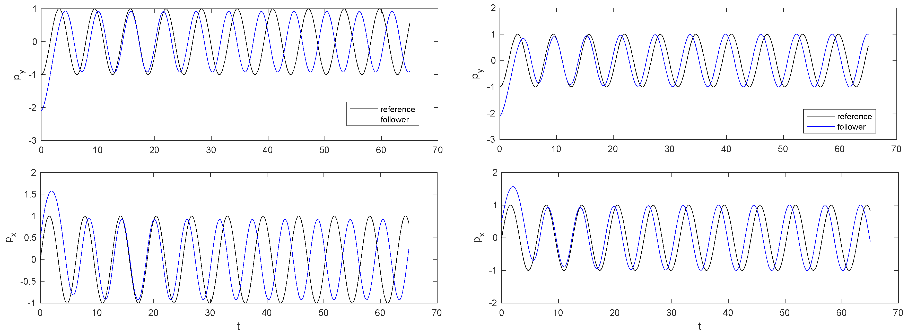
Figure 1 (left) shows the vehicle behavior (blue on the Figures) when applying $u=u_0$ the proportional controller derived for the nominal model, or in other words (12) with $k_I=0$. After a short initial transient, the motion of the vehicle does converge to rotation on a circle centered at the origin, but not at the correct speed. Indeed, the tracking vehicle keeps accumulating a phase advance with respect to the reference. This is because, due to the bias, the controller thinks that it has not converged to the correct configuration yet, and keeps pushing. As a result, the symmetry of coordinated motion is broken: the relative configuration between the following vehicle and the reference is continuously changing, with macroscopic long-term effects. This is rather problematic for a controller whose very purpose is to stabilize coordinated motion.

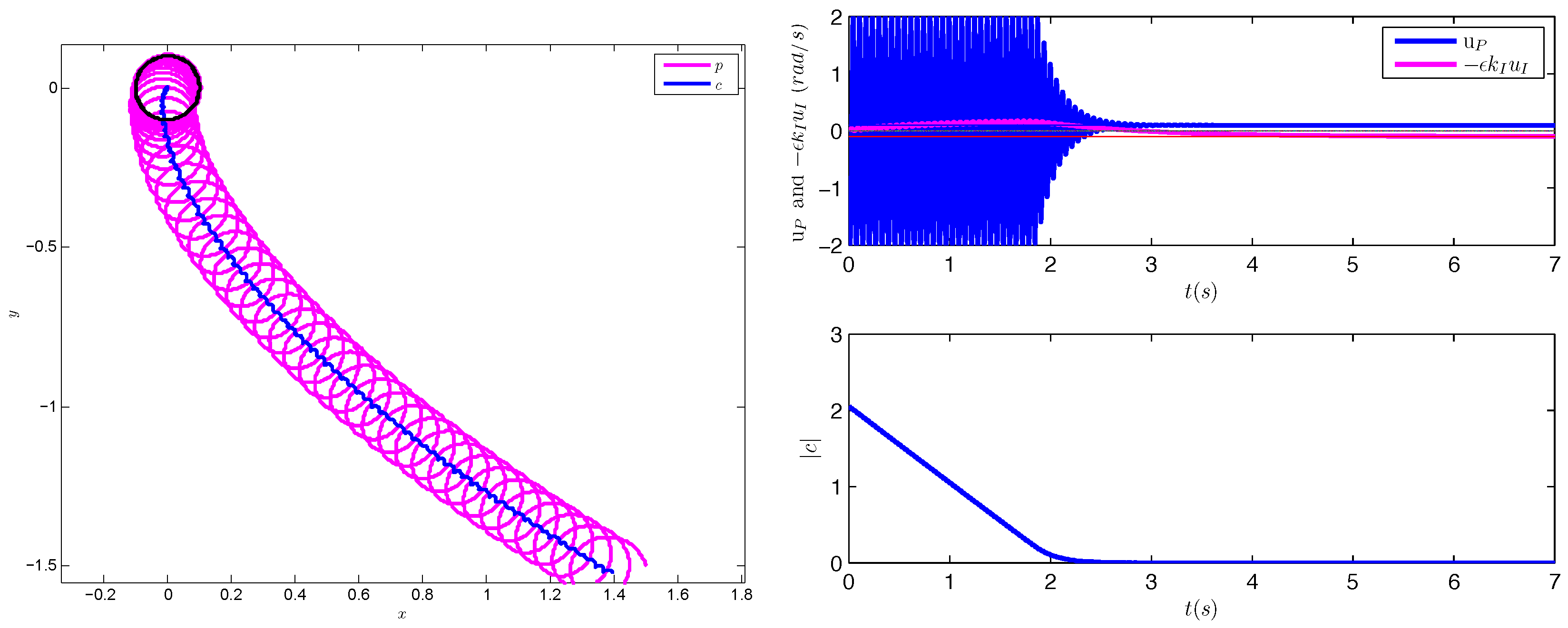
Our controller corrects this effect, as illustrated on Figure 1 (right) with tuning parameters $ϵk_P=1$, $ϵk_I=0.1$ and $\delta =0.2$. Indeed, after the initial transient during which the vehicle has to converge towards the correct circle, it moves with a fixed phase lag with respect to the reference, thus in coordinated motion. Figure 2 (left) shows a typical vehicle trajectory when starting farther away, and it confirms more visually that the vehicle converges to the correct circle (the fact that the vehicle is then rotating at the correct rate must be taken from other plots). Figure 2 (right) confirms the convergence of the true circle center $\mathbf{c}$ towards ${\mathbf{c}}^{\mathrm{ref}}=0$, which by definition (check (8) and the corresponding remark) should mean that it is rotating at the correct rate on the correct circle. The convergence is first linear due to the feedback saturation, then exponential once $|\mathbf{c}|<\delta$. The figure also shows that, while $u_P$ still thinks that it has to apply a correction (due to the bias between the true $\mathbf{c}$ and the $\widehat{\mathbf{c}}$ computed with the assumption $\mathbf{v}={\mathbf{e}}_1$ by the controller), the modified integral controller progressively understands that it has to cancel it such that the total control input reduces to $u={\omega }_{\mathrm{ref}}$.

We next include an unknown bias on the angular velocity too. The rotation velocity of the vehicle thus now corresponds to

$$\begin{array}{ccc}\hfill \omega & =& u+{\omega }_B={\omega }_{\mathrm{ref}}+u_P-k_I{u}_I+{\omega }_B\hfill \\ & =& {\omega }_{\mathrm{ref}}+(u_P\left(g^{-1}{g}_{\mathrm{ref}}\right)-u_P\left(\tilde{h}\right))-k_I{u}_I+u_P\left(\tilde{h}\right)+{\omega }_B.\hfill \end{array}$$

The total effective bias thus now corresponds to $u_P\left(\tilde{h}\right)+{\omega }_B$ instead of just $u_P\left(\tilde{h}\right)$. In other words, if we can drive $g^{-1}{g}_{\mathrm{ref}}$ towards $\tilde{h}$ and $-k_I{u}_I+u_P\left(\tilde{h}\right)+{\omega }_B$ towards 0, then we reach a perfect coordinated motion. It is tempting to view ${\omega }_B$ and $u_P\left(\tilde{h}\right)$ as just two similar contributions to the total bias, and thus by analogy we would just use the integral controller $\frac{d}{dt}{u}_I=u_P\left(g^{-1}{g}_{\mathrm{ref}}\right)-k_I{u}_I+{\omega }_B.$ The issue is that the controller a priori does not have access to the value of ${\omega }_B$. However, the controller does observe the relative heading $\theta \left(t\right)-{\omega }_{\mathrm{ref}}t$ of the vehicle with respect to the reference. Remarkably, since $\frac{d}{dt}\theta \left(t\right)=\omega$, we see that the integral term which we want to use in fact just corresponds to

$$u_I\left(t\right)=\theta \left(t\right)-{\omega }_{\mathrm{ref}}t.$$

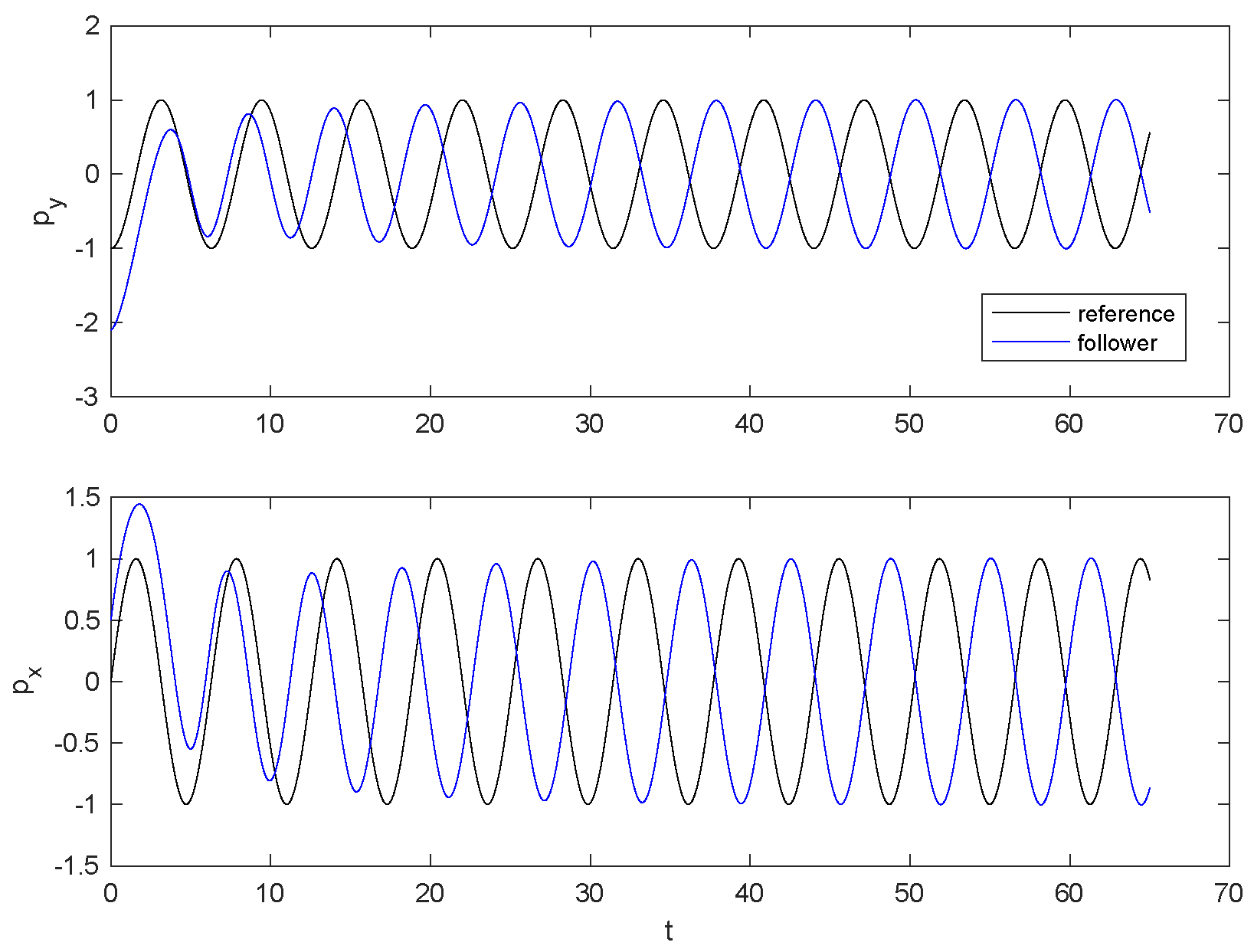
Thus, for the particular application of steering control, the general strategy in fact simplifies to feeding back a directly observed quantity. Figure 3 shows a simulation of this situation, with thus now biases on all velocities. We observe that the proposed modified integral controller indeed restores the symmetry of coordinated motion perfectly. The presence of ${\omega }_B$, with all other parameters and initial values kept as before, just translates into a different steady-state relative phase between reference and leader vehicle.

5. Towards Other Applications of the Modified Integral Controller

The modified integral controller (6) may have other applications. We briefly discuss this in a more abstract system-theoretic context.

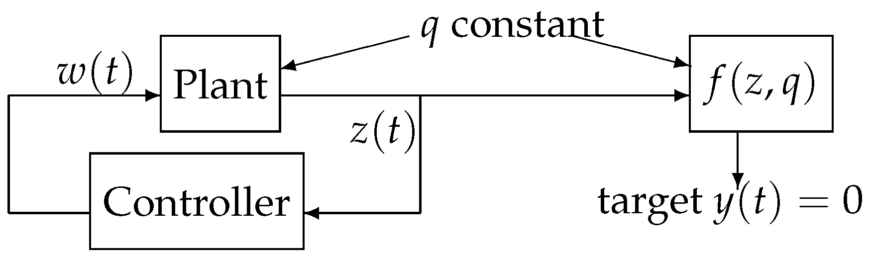
Consider the following abstract setting, see Figure 4:

• a system with state $x\left(t\right)$, variable of interest $y\left(t\right)$, must be stabilized to some target $(y,w)=0$ by the control command $w\left(t\right)$.
• unlike standard, the value of $y\left(t\right)$ is not measured, but deduced from actual measurements $z\left(t\right)$ through the static function $y=f(z,q)$ where q are some constant parameters.
• the exact value of q is not known; without loss of generality, $q=0$ is nominal and $f(0,0)=0$.

The target variable y is thus not available to the controller, while w is known. This setting could appear in various applications, as a consequence of a residual calibration error or of a sensor fault. The stabilization of coordinated motion can be formulated in this framework with

• x the rigid body configuration g, for the planar vehicle $(p,\theta )$;
• w the part of the input that corrects w.r.t. the target steady state motion, thus $u-u_{\mathrm{ref}}=\omega -{\omega }_{\mathrm{ref}}$ for the planar vehicle;
• $z=g^{-1}{g}_{\mathrm{ref}}$ the measured relative configuration between vehicle and reference, corresponding for the planar vehicle to $(Q^{-1}(p^{\mathrm{ref}}-p),{\theta }_{\mathrm{ref}}-\theta )=([z_1,z_2],z_3)$ with three scalar components;
• $q=u_B$ the parameter mismatch, corresponding to $\mathbf{v}-{\mathbf{v}}^{\mathrm{ref}}$;
• $y=\xi -{\mathrm{Ad}}_{g^{-1}{g}_{\mathrm{ref}}}{\xi }_{\mathrm{ref}}$ is the target variable to be put to zero, according to (4). For the vehicle, it has three scalar components $(Q^{-1}({\mathbf{c}}^{\mathrm{ref}}-\mathbf{c}),{\omega }_{\mathrm{ref}}-\omega )$. The last component is equivalent to $w=0$. Referring to (11), the others take the form

  $$\begin{array}{ccc}\hfill Q^{-1}({\mathbf{c}}^{\mathrm{ref}}-\mathbf{c})& =& Q^{-1}(p^{\mathrm{ref}}-p)+Q_{\pi /2}\frac{Q_{{\theta }_{\mathrm{ref}}-\theta }{\mathbf{v}}^{\mathrm{ref}}-\mathbf{v}}{{\omega }_{\mathrm{ref}}}\hfill \\ & =& [z_1,z_2]+Q_{\pi /2}\frac{Q_{z_3}{\mathbf{v}}^{\mathrm{ref}}-(q+{\mathbf{v}}^{\mathrm{ref}})}{{\omega }_{\mathrm{ref}}}=f(z,q),\hfill \end{array}$$
  indeed involving known constants, the unknown q, and observed variables z.

The goal is thus to propose a simple control mechanism which would automatically cancel the error on y associated with $q\ne 0$, without requiring advanced logic like an observer estimating sensor parameters.

We repeat a reasoning similar to the one of Section 2.3.

Assuming the nominal situation $q=0$, a well-tuned proportional feedback $w=u_P\left(z\right)$ would typically drive z to zero and thus y towards $f(0,0)=0$, at least locally. However, if $q\ne 0$, then $w=u_P\left(z\right)=0$ does not correspond to $y=0$ anymore. To perfectly reach the target $(y,w)=0$, the controller should instead apply

$$w=u_P\left(z\right)-u_P\left({\overline{z}}^{\left(q\right)}\right),$$

where ${\overline{z}}^{\left(q\right)}$ is a measurement value for which $f({\overline{z}}^{\left(q\right)},q)=0$. Because q is not known, the value of ${\overline{z}}^{\left(q\right)}$ is not known either. However, in this formulation, the effect of q can be viewed just as an unknown input bias $u_B=u_P\left({\overline{z}}^{\left(q\right)}\right)$ to be canceled.

A standard integral controller like (2) would require to integrate the true error y, which here is not measured. The hope is then to correct the situation by integrating instead the input corrections w. Indeed, the target includes the requirement $w=0$; and, if the effect of $q\ne 0$ is observable on z (and this is an important requirement), then by monitoring the corrections that we apply we should learn something about q. This motivates the same modified integral controller as proposed for coordinated motion:

$$\begin{array}{cc}\hfill & w=u_P-k_I{u}_I,\hfill \\ \hfill & \frac{d}{dt}{u}_I=w.\hfill \end{array}$$

(20)

If this controller reaches a steady state, then we have achieved half our goal namely $w=0$. A further observability/invariance property of the plant is necessary to ensure that we stabilize the full target. Namely, if states with $(w=0,z\ne {\overline{z}}^{\left(q\right)})$ are not invariant, while $(w,z-{\overline{z}}^{\left(q\right)})=0$ is invariant, then we can hope to show convergence towards $f(z,q)=f({\overline{z}}^{\left(q\right)},q)=0$ and $k_I{u}_I=u_B$.

This last requirement shows that (20) is likely to work, in general, if $(w,y)=0$ is a natural equilibrium and the purpose of the controller is to stabilize it, while avoiding that the feedback based on measurement z displaces the natural equilibrium from $y=0$.

We can make this more explicit on a linear system. Consider in Laplace domain

$$z\left(s\right)=y\left(s\right)+q\left(s\right)=H\left(s\right)\left(w\right(s)+b(s\left)\right)+q\left(s\right)$$

where the goal is to stabilize $y\left(s\right)=0$, while $b\left(s\right)$ is some actuation noise and $q\left(s\right)$ is noise on the output measurement [6]. With a controller $w\left(s\right)=C\left(s\right)z\left(s\right)$, we obtain the closed-loop equation

$$y\left(s\right)=\frac{H\left(s\right)C\left(s\right)}{1-H\left(s\right)C\left(s\right)}q\left(s\right)+\frac{H\left(s\right)}{1-H\left(s\right)C\left(s\right)}b\left(s\right).$$

(21)

For $C\left(s\right)=0$, the measurement noise is of course not transmitted to y. However, a controller might be necessary for stabilizing the system or rejecting disturbances b according to frequency-dependent specifications.

At each frequency, strongly attenuating the effect of b requires a large value of $HC$, which implies that q is transmitted into y with almost unit gain. Thus, to perfectly counter a bias in the input, you must be able to trust the value of the measurement, and vice versa. A standard proportional-integral controller makes $|C\left(s\right)|=|k_I/s+k_P|$ infinite at zero frequency, implying perfect rejection of $b\left(0\right)$. Conversely, our modified integral controller is well-adapted to applications where q poses major problems at low frequencies while $b\left(0\right)$ is low. Indeed, the MIC with $u_P=K\left(s\right)z$ writes

$$C\left(s\right)=\frac{K\left(s\right)s}{s+k_I}.$$

For frequencies $|s|\gg k_I$, we have $C\left(s\right)\simeq K\left(s\right)$. For small s, however, the controller is attenuated, and in particular when $H\left(0\right)K\left(0\right)$ is finite the MIC ensures $\frac{H\left(0\right)C\left(0\right)}{1-H\left(0\right)C\left(0\right)}=0$ i.e., perfect rejection of $q\left(0\right)$. The stability analysis must (only) investigate the changes implied at those low frequencies. Practical situations where it is relevant to reject $q\left(0\right)$ rather than $b\left(0\right)$ could appear when drifts of the sensor-zero cannot be calibrated, e.g., a shift induced by a failure event or by fluctuations of operating conditions.

Remark 2.

The integrator with leakage as used in [17] would instead yield

$$C\left(s\right)=\frac{K\left(s\right)(s+a)+k_I}{s+a}$$

with $a\ge 0$ the leakage parameter. For $a=0$, one recovers an integral controller. For large a, we get $C\left(s\right)\simeq K\left(s\right)$ at all frequencies. This does a priori not guarantee any specific transmission property for $q\left(s\right)$; the purpose of a leaking integrator is indeed rather to ensure more robust stability.

6. Conclusions

In this paper, we have investigated how a simple modified integral control (MIC) allows for restoring perfect coordination symmetry in the motion of steering controlled vehicles subject to actuation bias. The non-holonomic dynamics of such systems make it impossible to directly counter the bias. However, the conditions for perfect symmetry to be achievable are clear in a Lie group framework, and an adaptation of integral control to this situation is proved to yield perfect global convergence.

This control perspective on symmetry, more particularly on restoring it, seems to rely on stabilizing a manifold of configurations where symmetry holds, rather than formulating the problem directly as a tracking task. We have also discussed how this MIC might address other tasks, related to biases in output measurements. The common framework is that the target situation would be a natural equilibrium of the system, a feedback control action is used in order to stabilize it, and we must avoid that errors in the model used by the controller displace the steady state from the target situation.

Of course, more powerful state-based methods could also be devised, explicitly estimating all the model errors and biases and specifying according actions—see, e.g., [15]. However, much like for standard integral control, we believe that simple control “gadgets” like the MIC can have their own interest in terms of plug-and-play robustness (no need for an extensive system model in the controller), simplicity of implementation (e.g., in analog hardware), and therefore maybe providing insight into how some natural systems could be wired in order to preserve perfect symmetries. Also note that, like standard integral control, the strategy should remain applicable if the bias is state-dependent, which would be harder to formulate with explicit estimation.

References

- Bai, H.; Arcak, M.; Wen, J.T. Rigid body attitude coordination without inertial frame information. Automatica 2008, 44, 3170–3175. [Google Scholar] [CrossRef]
- Sarlette, A.; Sepulchre, R.; Leonard, N. Autonomous rigid body attitude synchronization. Automatica 2009, 45, 572–577. [Google Scholar] [CrossRef] [Green Version]
- Leonard, N.; Paley, D.; Lekien, F.; Sepulchre, R.; Frantantoni, D.; Davis, R. Collective motion, sensor networks and ocean sampling. Proc. IEEE 2007, 95, 48–74. [Google Scholar] [CrossRef]
- Justh, E.W.; Krishnaprasad, P. Equilibria and steering laws for planar formations. Syst. Control Lett. 2004, 52, 25–38. [Google Scholar] [CrossRef] [Green Version]
- Sepulchre, R.; Paley, D.A.; Leonard, N.E. Stabilization of planar collective motion: All-to-all communication. Autom. Control IEEE Trans. 2007, 52, 811–824. [Google Scholar] [CrossRef]
- Aström, K.J.; Murray, R.M. Feedback Systems: an Introduction for Scientists and Engineers; Princeton University Press: Princeton, NJ, USA, 2010. [Google Scholar]
- Zhang, Z.; Alain, S.; Zhihao, L. Integral control on Lie groups. Syst. Control Lett. 2015, 80, 9–15. [Google Scholar] [CrossRef] [Green Version]
- Maithripala, D.; Berg, J.M. An intrinsic PID controller for mechanical systems on Lie groups. Automatica 2015, 54, 189–200. [Google Scholar] [CrossRef]
- Hanssmann, H.; Leonard, N.; Smith, T. Symmetry and Reduction for Coordinated Rigid Bodies. Eur. J. Control 2006, 12, 176–194. [Google Scholar] [CrossRef] [Green Version]
- Sarlette, A.; Bonnabel, S.; Sepulchre, R. Coordinated motion design on Lie groups. IEEE Trans. Autom. Control 2010, 55, 1047–1058. [Google Scholar] [CrossRef]
- Aeyels, D.; Peuteman, J. On exponential stability of nonlinear time-varying differential equations. Automatica 1999, 35, 1091–1100. [Google Scholar] [CrossRef]
- Bonnabel, S.; Martin, P.; Rouchon, P. Symmetry-preserving observers. IEEE Trans. Autom. Control 2008, 53, 2514–2526. [Google Scholar] [CrossRef]
- Lageman, C.; Trumpf, J.; Mahony, R. Gradient-like observers for invariant dynamics on a Lie group. IEEE Trans. Autom. Control 2010, 55, 367–377. [Google Scholar] [CrossRef]
- Khosravian, A.; Trumpf, J.; Mahony, R.; Lageman, C. Observers for invariant systems on Lie groups with biased input measurements and homogeneous outputs. Automatica 2015, 55, 19–26. [Google Scholar] [CrossRef] [Green Version]
- Aguiar, P.; Hespanha, J. Trajectory-tracking and path-following of underactuated autonomous vehicles with parametric modeling uncertainty. IEEE Trans. Autom. Control. 2007, 52, 1362–1379. [Google Scholar] [CrossRef]
- Sanders, J.A.; Verhulst, F.; Murdock, J. Averaging Methods in Nonlinear Dynamical Systems; Springer: Berlin, Germany, 1985. [Google Scholar]
- Gorinevsky, D.; Boyd, S.; Stein, G. Design of low-bandwidth spatially distributed feedback. IEEE Trans. Autom. Control. 2008, 53, 257–272. [Google Scholar] [CrossRef]
Figure 1.
Left: Evolution of position p over time with nominal-case controller (): reference (black) and actual motion (blue) undergo a progressive dephasing, i.e., a small calibration error breaks the symmetry of coordinated motion. Right: Evolution of position p over time with our modified integral controller: the perfect coordinated motion of reference (black) and actual motion (blue) is restored.
Figure 2.
With modified integral control, left: trajectories of position p and center . Right: convergence of the proportional input , integral input and deviation of circle center . On the upper right plot, horizontal lines are provided as guides to the eye to witness that the integral input asymptotically cancels the remaining .
Figure 3.
Evolution of position p over time with our modified integral controller, when adding as well an actuation bias on the actuated part of the velocity. This corresponds to biases everywhere, and the correcting integral controller appears to boil down to . The perfect coordinated motion of reference (black) and actual motion (blue) is restored in that case too.
Figure 4.
Abstract problem setting to stabilize .
© 2019 by the authors. Licensee MDPI, Basel, Switzerland. This article is an open access article distributed under the terms and conditions of the Creative Commons Attribution (CC BY) license (http://creativecommons.org/licenses/by/4.0/).
Share and Cite
MDPI and ACS Style
Zhang, Z.; Ling, Z.; Sarlette, A. Modified Integral Control Globally Counters Symmetry-Breaking Biases. Symmetry 2019, 11, 639. https://doi.org/10.3390/sym11050639
AMA Style
Zhang Z, Ling Z, Sarlette A. Modified Integral Control Globally Counters Symmetry-Breaking Biases. Symmetry. 2019; 11(5):639. https://doi.org/10.3390/sym11050639
Chicago/Turabian StyleZhang, Zhifei, Zhihao Ling, and Alain Sarlette. 2019. "Modified Integral Control Globally Counters Symmetry-Breaking Biases" Symmetry 11, no. 5: 639. https://doi.org/10.3390/sym11050639
Note that from the first issue of 2016, this journal uses article numbers instead of page numbers. See further details here.