Calculation Method of Material Accumulation Rate at the Front of Trunk Glaciers Based on Satellite Monitoring

Abstract

Glaciers continue to erode and transport material, forming an accumulation area at the front of the glacier. The trunk glacier, which has many tributary glaciers upstream and converges on the main channel, deposits vast amounts of material in the main channel. It blocks the main channel, forming barrier lakes, and eventually turns into mountain disasters, such as debris flows or outburst floods. Therefore, the accumulation rate of the material is a major parameter in such disasters and can determine the frequency of disasters. The material usually comes from bedrock erosion by glaciers, weathering of bedrock walls, and upstream landslides, and the material loss depends on river erosion. Based on this, we set up a method to calculate the material accumulation rate in the glacier front based on satellite images. Then, the Peilong catchment was taken as an example to validate the proposed method. The results indicate that climatic fluctuations may increase landslides, resulting in more actual accumulation than the calculated value according to the average rate of bedrock retreat. The material provided by the retreat of bedrock accounts for 92% of the total volume. Our method provides a practical reference for the mid- and long-term prediction of glacial catastrophic mass movement, as global warming seriously threatens glacier instability and downstream communities.

1. Introduction

Alpine mountains with sufficient water vapor are often occupied by maritime glaciers, which move fast and accumulate material continuously at the glacier front, thereby supplying the loss material for mountain disasters, such as debris flows and outburst floods. In general, the faster the accumulation rate is, the higher the frequency of disasters. Therefore, the rate is particularly important. However, it is difficult to measure due to the high altitude and difficult access. Moreover, limited by small monitoring areas, image accuracy, shelter, and other problems, remote sensing interpretation also has difficulty obtaining accurate results. Therefore, it is necessary to propose a new method to calculate the material accumulation rate.

The material at the front of glaciers is usually transported by glaciers, and the source of the material contains bedrock erosion by glaciers and bedrock retreat. Therefore, the glacier erosion rate and bedrock retreat rate play key roles in the material accumulation rate. Due to the differences in glacier characteristics, location, topography, etc., the glacier erosion rate spans four orders of magnitude from polar glaciers to maritime glaciers [1,2,3]. There are three methods to calculate the glacier erosion rate [4]: (1) geomorphological reconstruction, which calculates the erosion rate based on the ancient landform estimated by the existing geomorphology and overburden; (2) sediment estimation, which calculates the erosion rate based on Quaternary sediment; and (3) a physical calculation model is the third method of calculating the glacial erosion rate. Due to the imbalance of glaciers in time [5,6] and space [7], the first two methods have difficulty reaching a consistent conclusion. The physical model requires many parameters with a complicated calculation process [8,9]. Therefore, these calculation methods have some defects.

There are bedrock slopes in addition to glaciers in glaciated areas that provide material by weathering. In addition, deglaciation causes some bedrock slopes to lose lateral support, resulting in landslides. The initial landslides occur shortly after deglaciation and are then associated with stress release [10]. Many scholars have studied the bedrock retreat process [11,12] and found that bedrock retreat is accompanied by surface weathering and deep landslides, and the rates of the two are different. The weathering rate in the Alps is 0.1 mm/a [13], which is an order of magnitude lower than the long-term retreat rate (1–2 mm/a) containing weathering and landslides in the area [14,15]. The global average rate of bedrock retreat in alpine mountains is 1.1 mm/a [16].

Based on previous studies, we focus on trunk glaciers by combining the material supply and decrease to research the rate of material accumulation, which provides a theoretical basis for studying glacial debris flows and outburst floods.

2. Methods

2.1. Material Accumulation Rate

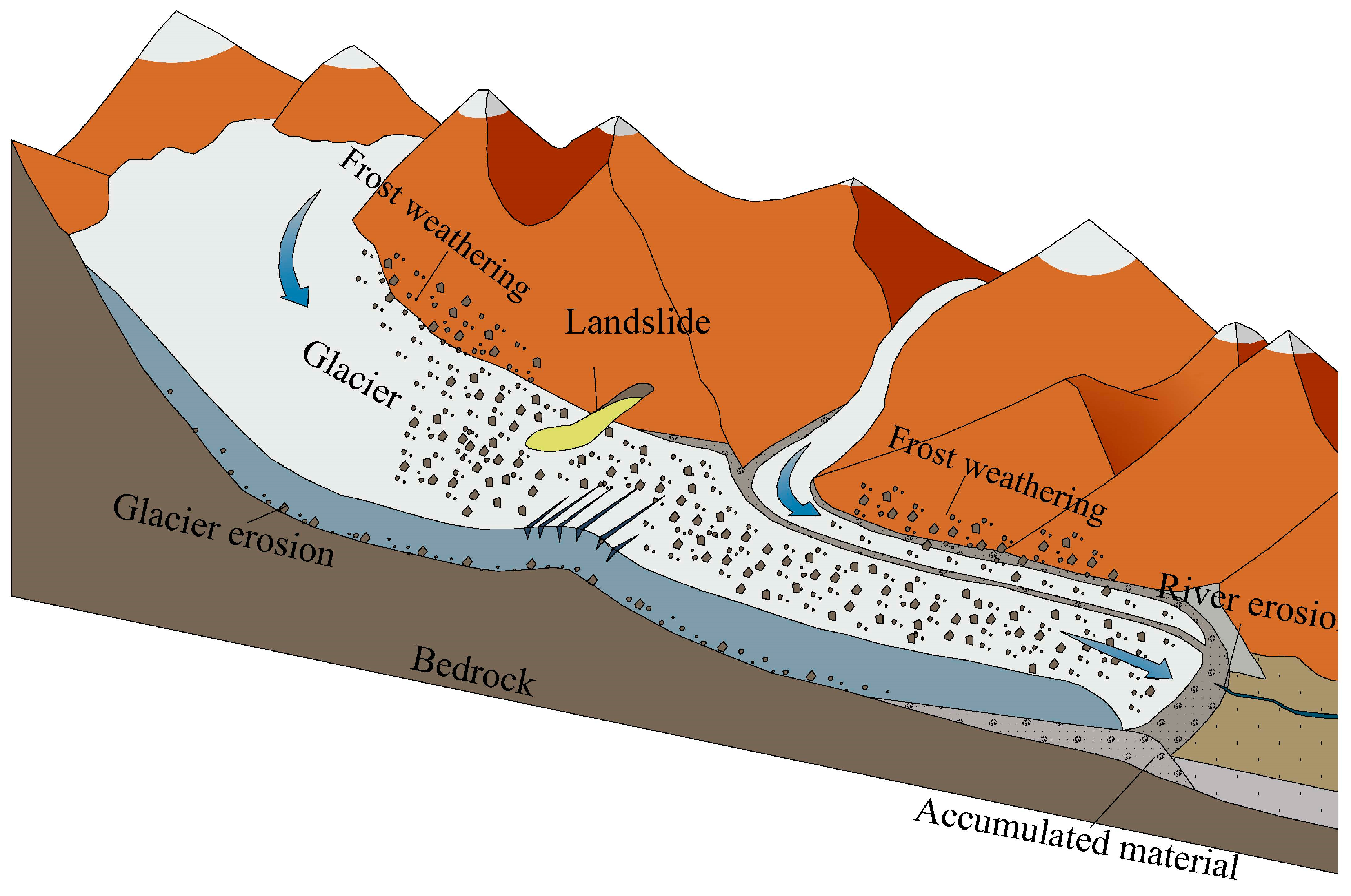
The material at the glacier front is supplied by 2 phenomena, namely, glacier erosion and bedrock retreat, and the decrease in material is due to long-term river transport and sudden debris flow transport (Figure 1). We ignored sudden material consumption, such as that which occurs in debris flows; therefore, we mainly considered the material accumulation rate between two debris flows. Considering the relationship between different processes, we established a model of the material accumulation rate (Formula (1)), which is represented by the change in material volume (V) with time (t).

$$\frac{\partial V}{\partial t}=E+W-{\Phi }_F$$

(1)

where E is the average annual erosion rate of the glacier (m³/a); W is the material accumulation rate caused by bedrock retreat (m³/a); and ${\Phi }_F$ is the average annual erosion rate of the river (m³/a). Formula (1) is based on the assumption that the supply and decrease in materials in each process is constant. Therefore, the following three conditions need to be met:

(1)

On a large time scale, the glacier shape and glacier erosion rate are constant.

(2)

On a large time scale, the retreat rate of bedrock is constant, and the material supplied by bedrock retreat is always transported to the glacier front by glaciers.

(3)

In the absence of sudden external processes, such as earthquakes and debris flows, the material supply is controlled by glacier erosion and bedrock retreat, and the material decrease is eroded by rivers.

2.2. Glacier Erosion Rate

The glacier erosion rate varies by four orders of magnitude from polar glaciers to maritime glaciers [1,2,3], which is due to the varying velocities of different glaciers, and the glacier erosion rate is proportional to the velocity [17,18,19]. Herman et al. [20] studied the relationship between glacier velocity and erosion rate, obtaining a nonlinear function. The glacier erosion rate can be expressed by Formulas (2) and (3).

$$E=\sum _{i=1}^n{A}_i{e}_i$$

(2)

$$e_i=K_g{\left|u_i\right|}^l$$

(3)

where $A_i$ is the glacier area (m²); $e_i$ is the glacier erosion depth (m/a); K_g is the erosion constant (${\mathrm{m}}^{1-\mathrm{l}}/{\mathrm{a}}^{1-l}$); $u_i$ is the glacier velocity (m/a); and l is the index.

Glacier velocity can be measured with two kinds of methods, including ground observation using instruments with high temporal–spatial resolution [21,22] and large-scale velocity detection from remote sensing imagery [23,24]. In the past two decades, remote sensing methodology has been increasingly used to extract glacier velocities because of its convenient access and improved accuracy. There are three kinds of methods used to extract glacier velocity, namely, Synthetic Aperture Radar (SAR) amplitude-based offset tracking, SAR phase shift analysis, and optical cross-correlation offset tracking. These methods have their own advantages and disadvantages when applied to glacier deformation or velocity extraction. This study extracts the interannual glacier velocity that is easily captured via optical images because of its large deformation feature. Therefore, we applied optical cross-correlation offset tracking to estimate the glacier velocity before the development of the debris flow. This method first selects two images with the same location and short intervals. Then, the feature point in the two images is tracked to calculate the distance. Finally, the velocity of the feature point is calculated with the point distance and the interval time of the images. This process can be calculated using open source software named COSI-corr. The time interval between the two images should not be overly large; otherwise, the feature points may deform and not be tracked. Additionally, the image should have no occlusions, such as clouds.

2.3. Bedrock Supply Rate

The bedrock in the glacial zone provides a large amount of material via two ways: frost weathering and landslides. The material is transported by the glacier and accumulates at the glacier front. Although the two processes are not uniformly distributed in space, they occur slowly at a certain rate in the long term.

The material volume supplied by bedrock retreat is controlled by the bedrock area and the retreat rate. Therefore, we use Formulas (4) and (5) to express the volume.

$$W=e{A}_B$$

(4)

$$A_B={A-A}_I$$

(5)

where e is the bedrock retreat rate (m/a); $A_B$ is the bedrock area that supplies loose material (m²); $A_I$ is the glacier area in the glacial zone (m²); and $A$ is the drainage contribution area of the glacier front (m²).

2.4. River Erosion Rate

In addition to the sudden large-scale transport of debris flow material, the decrease in material is mainly caused by river erosion. River erosion is a long-term process, and its transport capacity is related to river power [25]. According to Martin and Church [26] and Dadson and Church [27], the river erosion rate can be expressed by Formula (6).

$${\Phi }_F=\left\{\begin{array}{l}6.44Q^{0.35}{S}^{1.5} \mathrm{i}\mathrm{f} S<0.22\\ 40.32Q^{0.34}{S}^{2.22} \mathrm{i}\mathrm{f} 0.22\le S\le 0.3\\ 0 \mathrm{i}\mathrm{f} S>0.3\end{array}\right.$$

(6)

where ${\Phi }_F$ is the river erosion rate (m³/a); Q is the river discharge (m³); and S is the gradient of the river.

The most accurate method of river discharge monitoring is via hydrographic stations. However, river discharge is hard to monitor due to the high altitude and complicated environment. Therefore, when river discharge measurements are not possible, it is necessary to propose a new method for calculating discharge. Lv et al. [28] studied the river discharge in the Parlung Zangbo Basin and believed that the river discharge could be calculated by analogy. They believe that in a region, there are two important ratios: the ratio of glacial meltwater to river discharge (R₁) and the ratio of glacier area to drainage contribution area (R₂). The ratio of R₁ to R₂ is nearly equal in different basins. Therefore, the river discharge can be calculated by the glacier area, glacial meltwater discharge, and the known ratio. According to Lv et al. [28], the average annual melting depth of glaciers is almost equal to that at the snow line, and then they can be calculated by Formulas (7) to (9).

$$h_I=1.33{\left(9.66+t_s\right)}^{2.85}$$

(7)

$$h_w=h_I{\rho }_I∕{\rho }_w$$

(8)

$$Q_I=A_I{h}_w$$

(9)

where $h_I$ is the average annual melting depth of glaciers (mm); $h_w$ is the water depth transformed by the glacier melting depth (mm); $t_s$ is the temperature from June to August at the snow line (°C); ${\rho }_I$ and ${\rho }_w$ are the densities of glaciers and water (g/cm³), respectively; and $Q_I$ is the glacier discharge by glacier melting (m³/a).

According to Lv et al. [28], the ratio of R₁ to R₂ is 1.27. The ratio of glacial meltwater to the river discharge at a point in the target basin is calculated by Formula (10), and the discharge at the point is obtained by Formula (11).

R₁ = 1.27 × R₂

(10)

$$Q ={ Q}_I/{\mathrm{R}}_1$$

(11)

2.5. Calculation Process

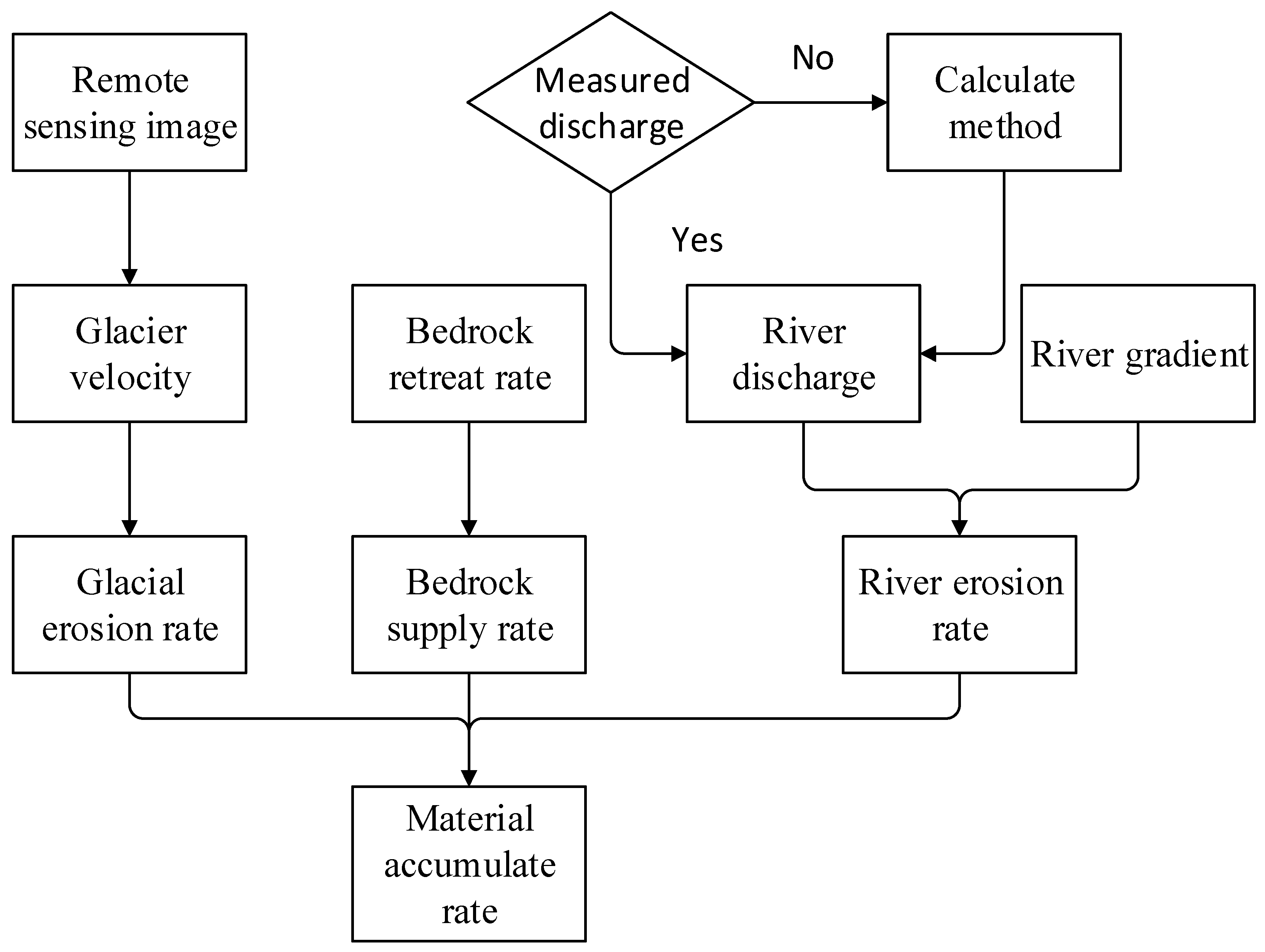
We summarized the general process for calculating the material accumulation rate, and it is shown in Figure 2. First, the cloud-free satellite images were paired up and used to estimate the distance of glacier movement between before and after the paired image date. This glacier movement distance in each year was then transformed into glacier velocity with units of m/a. Consequently, the glacial erosion rate was calculated via glacier velocity. Second, we used historical images to map the boundaries of glaciers to determine the exposure rate of moraines. In addition, landslides and rock falls in glacier-covered areas were interpreted. These two parts of materials were used to indicate the bedrock supply rate. Third, we used the glacier meltwater equivalent to estimate the material transport rate. With the above step, the material accumulation rate was eventually calculated.

3. Background of the Verification Case

3.1. Glacier Geomorphology and Historical Debris Flows

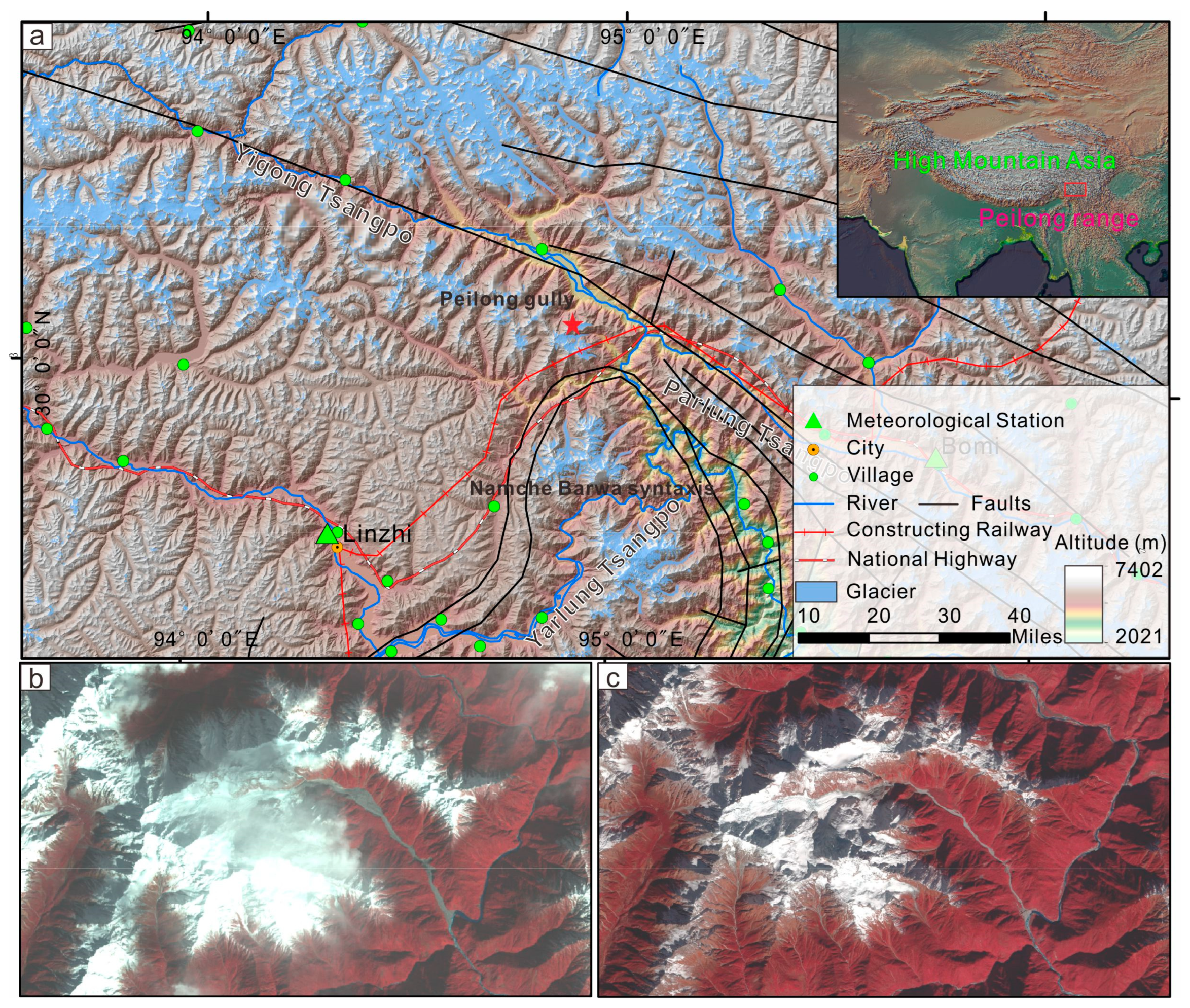
We chose the Peilong catchment (94°59′23″ E, 30°04′13″ N) for the calculation. The Peilong catchment is located downstream of the Parlung Zangbo basin (Figure 3), which is only approximately 21 km away from the outlet. This crescent-shaped catchment is 85.55 km². The main channel is 18.75 km long, and the channel gradient is 13.2%. The elevation ranges from 1984 to 5685 m, with a relative relief of 3701 m. Maritime glaciers extend between 3100 m and 5686 m in the Peilong catchment, with a total area of approximately 20.68 km².

Prior to 1983, only a few debris flows occurred in the Peilong catchment. A gradual increase in debris flow activity since 1983 has resulted in the destruction of parts of national highway 318 many times, blockage of the Parlung Zangbo, and strong erosion of the left bank of the river.

On 28 July 1983, a glacial avalanche on the right side of the glacier tongue formed a depositional dam 260 m high and 3 km long that blocked the channel, and a glacial lake of 5.0 × 10⁶ m³ ponded upstream. The glacial debris flow began at approximately 11 PM that day and lasted for approximately 10 h, with a peak flow of 2950 m³/s [29].

A glacier avalanche triggered 10 glacial debris flows in 1984, the largest of which was on 23 August and had a peak flow of 5245 m³/s [29]. The flow lasted for 23 h and blocked the Parlung Zangbo River for 15 min, raising the riverbed by 10 m, flooding the highway for 6 km, and forming a deposition fan of 5.0 × 10⁶ m³.

On 17 June 1985, a glacier avalanche induced an unstable slope to collapse, forming a dam with a maximum height of approximately 230 m and a width of approximately 1100 m. The dam included moraine and weathered rock blocks and probably incorporated the remains of past debris flow deposits at the base. The ensuing debris flow lasted three days with a peak discharge of 8195 m³/s [29]. The accumulation fan with a length of 440 m and width of 1135 m blocked the Parlung Zangbo River.

After 1985, there were very few debris flows in the Peilong catchment. After 1991, the catchment was stable until 17 August 2015, when a debris flow destroyed a steel bridge and blocked the Parlung Zangbo again.

3.2. Data Collection

Current glacier monitoring mainly utilizes optical remote sensing. Here, we used a collection of optical images from multiple sensors to retrieve glacier information, including glacier velocity, glacier boundaries, and catastrophic debris flows, in the past half century to track the evolution of the channel.

Table 1. Remote sensing datasets used in this study.

Sensor/Program	Date (dd/mm/yyyy)	Number of Images	Resolution (m)	Revisit Period (Day)	Usage	Source *
Corona KH-4A	03/03/1967– 02/05/1968	2	3	-	Glacier mapping; debris flow identification	USGS
Hexagon KH-9	16/11/1973	1	6	-	Glacier mapping	USGS
Aster	18/11/2002–02/08/2015	12	15	-	Glacier mapping	USGS
Landsat 1	16/12/1972	1	60	-	Glacier mapping	USGS
Landsat 4–5	05/01/1988–04/11/2011	46	30	16	Glacier mapping	USGS
Landsat 7	24/09/1999–08/02/2021	13	30	16	Glacier and velocity extraction	USGS
Landsat 8	20/07/2013–16/02/2021	16	15/30	16	Glacier and velocity extraction	USGS
Sentinel 2A/B	12/06/2015–12/25/2018	32	10/60	5	Glacier and velocity extraction; landslide interpretation	ESA
GaoFen-1	11/18/2013–12/06/2019	13	2/8	-	Debris flow identification; landslide interpretation	CCRSDA
GaoFen-2	01/17/2016–12/26/2018	5	0.8/3.2	-	Debris flow identification; landslide interpretation	CCRSDA

* USGS—United States Geological Survey, https://earthexplorer.usgs.gov/ (accessed on 5 September 2022); ESA—European Space Agency, https://scihub.copernicus.eu/ (accessed on 21 March 2022); CCRSDA—China Centre for Resources Satellite Data and Application, http://www.cresda.com/EN/ (accessed on 11 May 2023).

lists the collected remote sensing datasets in this study.

4. Result

4.1. Parameters

The method for calculating the material accumulation rate includes many parameters. In terms of the glacier erosion rate, previous scholars believed that the glacier erosion rate has a linear relationship with the glacier movement velocity, that is, l = 1, K_g = 10⁻⁴ m/a. However, Herman et al. [20] found that there was a power rate relationship between them, and the parameters were obtained by fitting the process of glacier movement in the Southern Alps of New Zealand, as l = 2.02, K_g = 2.7 × 10⁻⁷ m^l−1/a^1−l. Bedrock retreat usually consists of two parts: rock falls dominated by surface frost weathering and bedrock landslides in relatively deep parts. The former is a continuous process of stable and slow bedrock denudation. The latter is an accidental sudden phenomenon, which suddenly increases the bedrock retreat rate in a short time. When the two processes span a large time scale, the bedrock wall usually presents a gradual retreat at a relatively average and stable rate. According to previous studies, the frost weathering rate of the Alps is 0.1 mm/a [13], which is an order of magnitude lower than the long-term retreat rate (1–2 mm/a) in the area [14,15]. The average rate of bedrock retreat in the global alpine mountains is 1.1 mm/a [16].

Table 2. Calculating the values of parameters.

Parameter	Symbol	Value	Source
Erosion constant	Kg	$2.7\times {10}^{-7}{\mathrm{m}}^{1-\mathrm{l}}/{\mathrm{a}}^{1-\mathrm{l}}$	Herman et al. [20]
Erosion index	l	2.02	Herman et al. [20]
Bedrock retreat rate	e	1.1 mm/a	Murton [16]
Weathering rate		0.1 mm/a	Matsuoka [13]
Temperature at the snow line during June to August	$t_s$	4.5 °C	Institute of Mountain Hazards and Environment, CAS [30]
Glacier density	${\rho }_I$	$900 \mathrm{k}\mathrm{g}∕{\mathrm{m}}^3$	Cuffey and Paterson [31]
Water density	${\rho }_w$	$1000 \mathrm{k}\mathrm{g}∕{\mathrm{m}}^3$
Proportion of meltwater	n	0.634	Lv et al. [28]

lists the values of parameters.

4.2. Glacier Erosion Rate

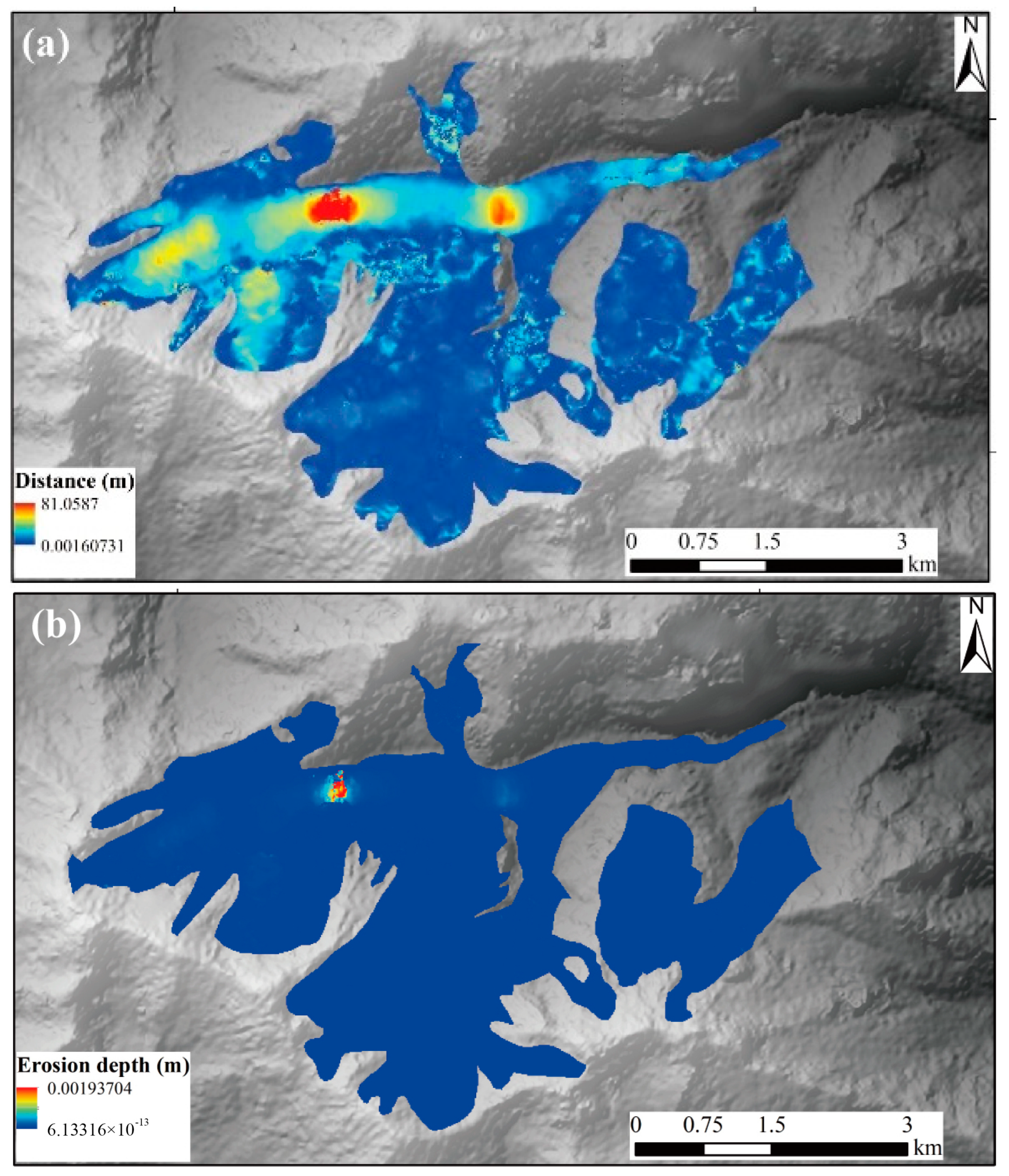
Through feature tracking, we obtained the velocity of glacier movement, and the corresponding erosion depth and erosion amount were converted according to the calculation of Formulas (2) and (3). Figure 4a shows the distance of glacier movement from 19 January to 18 February 2014, which can be considered the velocity of glacier movement per month. The monthly erosion depth of the glacier was obtained through Formula (3) (Figure 4b). Then, we obtained the monthly erosion volume with Formula (12), which was transformed by Formula (2) according to the grid area in ArcGIS 10.2 software (Environmental Systems Research Institute, Redlands, CA, USA).

$$V_m=\sum _{i=1}^n{d}_i{A}_{ci}$$

(12)

where $V_m$ is the monthly erosion volume of the glacier (m³); $d_i$ is the erosion depth of a cell (m); and $A_{ci}$ is the area of the corresponding cell. Since the data source was the 12.5 × 12.5 m resolution DEM from ALOS PALSAR, the area of each cell was 156.25 m². Therefore, the formula can be rewritten as Formula (13).

$$V_m=156.25\sum _{i=1}^n{d}_i$$

(13)

According to the above formula, the erosion volume of the glacier in the Peilong catchment from 19 January to 18 February 2014 is 223.90 m³. The glacier velocity increases as the temperature or rainfall increases. Therefore, the erosion rate of glaciers in summer is significantly larger. However, due to the absence of summer image data, it is impossible to know the glacier velocity in summer. The annual glacier erosion rate is 2686.80 m³ when we assume a constant rate.

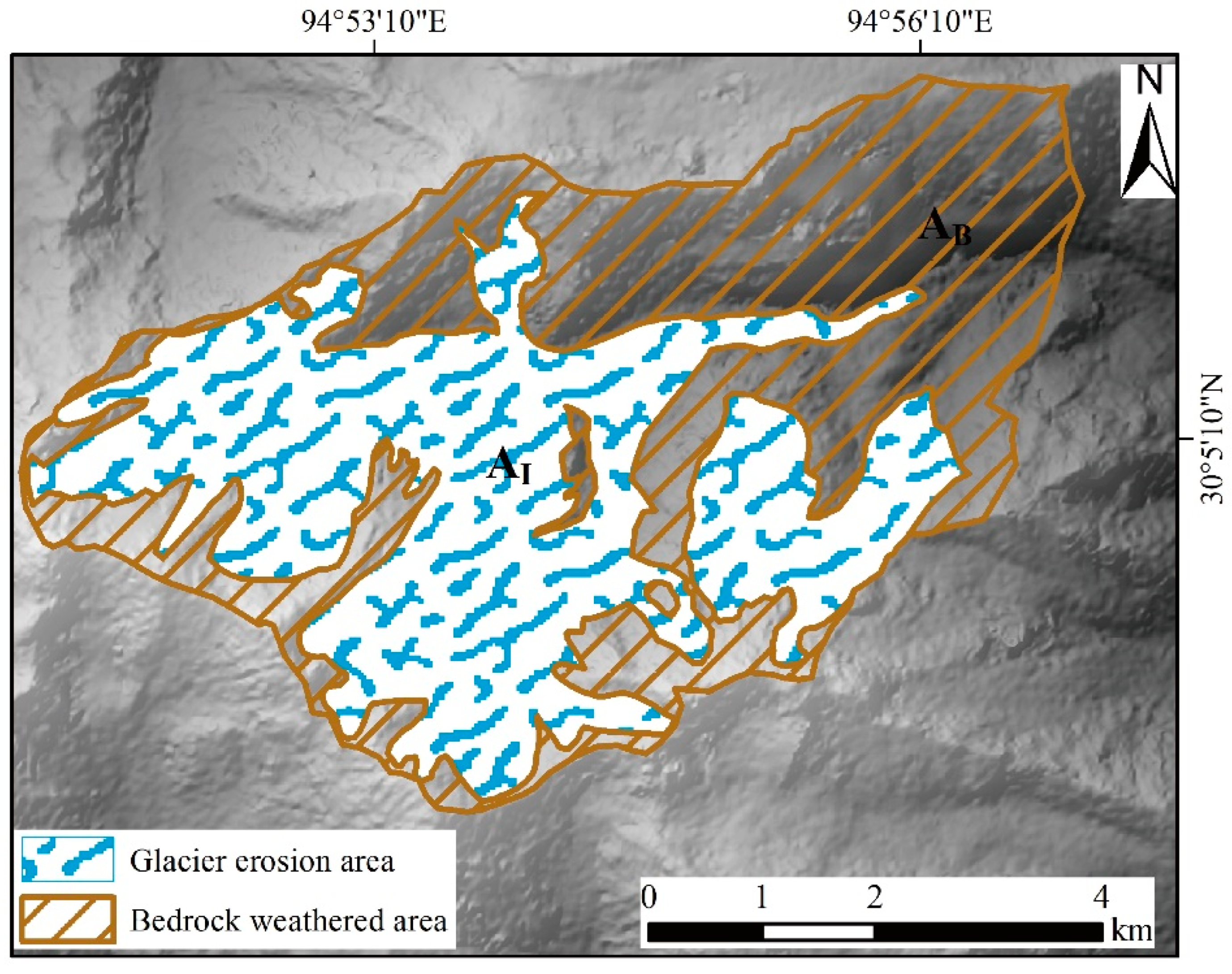
4.3. Bedrock Regression Rate

Based on the location of the glacier tongue, the upstream drainage contribution area (A) is 45.41 km², and the glacier area (${\mathrm{A}}_{\mathrm{I}}$) is 20.68 km², so the bedrock area (${\mathrm{A}}_{\mathrm{B}}$) is 24.73 km² (Figure 5). Since there are two types of bedrock retreat parameters, we calculated them separately. When using the average retreat rate, it is not necessary to consider the material supply provided by the landslide and collapse in the glacial area. Based on the global average retreat rate of 1.1 mm/a, the annual accumulation volume of material is 27,192 m³. The rate is an order of magnitude larger than the glacier erosion rate, which can be attributed to the following two reasons. First, the velocity of glacier movement is measured in the dry season, and it is smaller than that in the rainy season. Therefore, we obtained a relatively small erosion ability. Second, the average retreat rate of bedrock consists of the frost weathering rate, landslides, and other processes, which is an order of magnitude larger than the weathering rate. When we calculated the material accumulation of the bedrock according to the weathering rate, the annual accumulation volume was 2473 m³.

4.4. River Erosion Rate

Table 3. Parameters of the river transport rate.

Parameter	Glacier Melt Depth (m)	Transformed Depth of Water (m)	Meltwater Volume (m3)	Discharge (m3)	Gradient	Erosion Volume (m3)
Value	2537.36	2283.62	$4.12\times {10}^7$	$7.12\times {10}^7$	0.249	860.84

lists the parameters in the calculation of the river transport rate and the annual transport volume. The annual volume of glacial meltwater is 4.12 × 10⁷ m³ according to the glacier melting depth, and the total discharge at the glacier front is 7.12 × 10⁷ m³ combined with the ratio Factor n. The longitudinal gradient of the glacier front is 0.249. The annual erosion volume of the river at the glacier front is 860.84 m³, which is far less than the glacier erosion volume and frost weathering volume.

4.5. Total Material Accumulation Rate

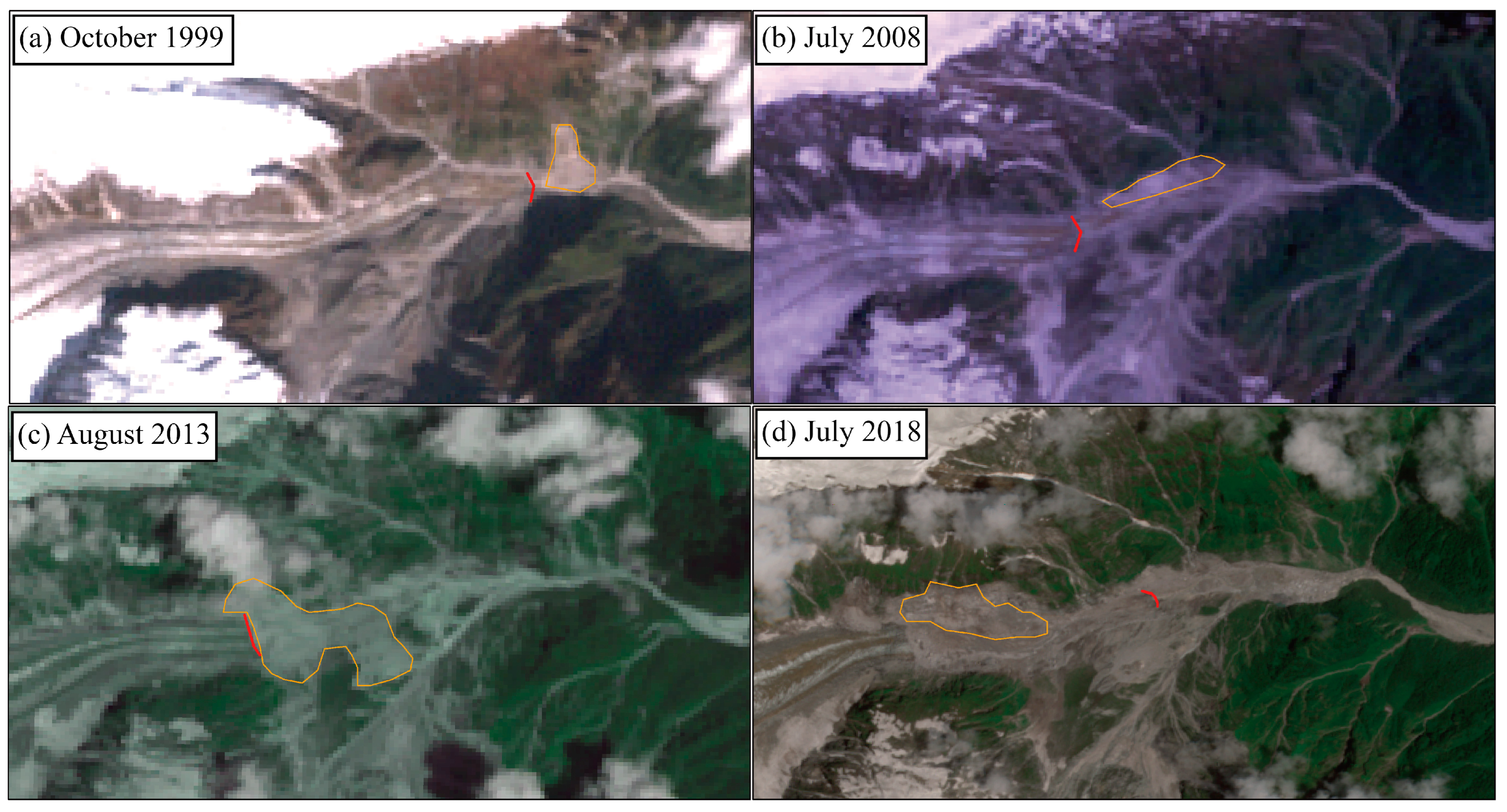
According to the average rate of bedrock retreat, the material accumulation rate at the glacier front in the Peilong catchment is 29,023.95 m³/a (

Table 4. Material accumulation rate and accumulation volume.

Parameter	Glacier Erosion Rate (m3/a)	Weather Rate (m3/a)	River Erosion Rate (m3/a)	Material Accumulation Rate (m3/a)	Material Accumulation Volume in 30 Years (m3)
Value	2686.80	27,192.00	860.84	29,017.96	$8.71\times {10}^5$

). Since 1985, the 30-year material accumulation volume at the glacier front was 8.71 × 10⁵ m³. If using the frost weathering rate, it is necessary to consider the volume of landslides and collapse. According to Wang et al. [32], three landslides occurred in the Peilong catchment in 1999, 2008, and 2013. We obtained the landslide volume by the relation of landslide volume-area ($V=\alpha A^{\gamma }$), where α = 0.146 and γ = 1.332 [33]. Finally, the total material accumulation volume was calculated based on the glacier erosion volume, frost weathering volume, river erosion volume, and landslide volume (

Table 5. Material volume calculated by the frost weathering rate and landslide volume.

Year	Landslide Area (m2)	Landslide Volume (m3)	Total Landslide Volume (m3)	Glacier Erosion Volume (m3)	Frost Weathering Volume (m3)	River Erosion Volume (m3)	Total Volume (m3)
1999	$1.14\times {10}^5$	$4.19\times {10}^5$	$8.64\times {10}^5$	$0.81\times {10}^5$	$0.74\times {10}^5$	$0.26\times {10}^5$	$9.93\times {10}^5$
2008	$0.34\times {10}^5$	$0.84\times {10}^5$
2013	$1.02\times {10}^5$	$3.61\times {10}^5$

).

By comparing the two sets of data, we found that the volume composed of frost weathering and landslides was larger than that of bedrock retreat, and the latter was approximately 12.3% smaller than the former. According to the calculation process and the environmental analysis of the Peilong catchment, we speculate that there are two reasons as follows. First, the parameters are inaccurate. The average retreat rate of bedrock is the average of the global alpine mountains, and the bedrock weathering rate is in accordance with the research of Matsuoka [13], who studied the frost weathering rate of the Alps and found it to be an order of magnitude smaller than the local rate of bedrock retreat. The volume-area relationship of landslides is also the average value obtained according to big data statistics. Therefore, all the parameters may not be applicable to the Peilong catchment. Second, the temperature in the Peilong catchment quickly increased after 2000 [32], and the glacier movement velocity also accelerated, which induced several landslides and increased the landslide volume.

4.6. Verification of the Results

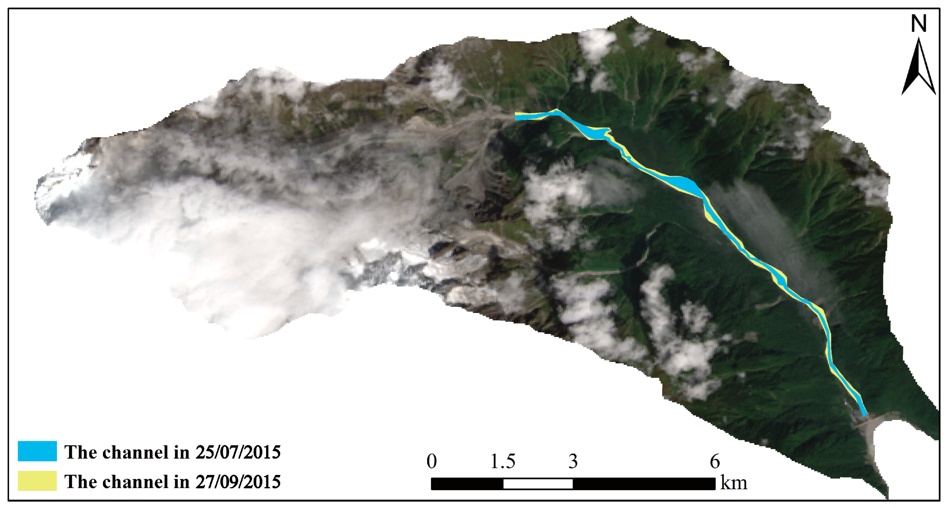
According to Wang et al. [32], a debris flow occurred on 17 August 2015, which was the first debris flow after 1985. This means that the 30 years of material loss of the glacier front is only due to river erosion. The debris flow initiated at the front of the glacier and was caused by the moraine blocking the channel. The debris flow eroded along the way, resulting in a constantly increasing volume of debris flow with an accumulated volume of approximately 4 × 10⁶ m³. After the debris flow, the river channel area increased by 4 × 10⁵ m² (Figure 6). And according to the field investigation, the channel erosion thickness of the debris flow was 8 m [32], which means that the material supplied by the erosion area was approximately 3.2 × 10⁶ m³ and material supplied by the initial area was approximately 8 × 10⁵ m³.

This result is slightly smaller than we calculated, with an error range of 9% to 24%. The error range is related to debris flows. A debris flow cannot transport all the material, and remote sensing images indicate that some material still exists in the initial area after the debris flow (Figure 6). Therefore, the calculated material volume is greater than the initial volume.

5. Discussion

The calculation shows that the material accumulation rate at the glacier front in the Peilong catchment is mainly caused by bedrock retreat, which includes frost weathering and landslides. The annual erosion volume of the glaciers in the Peilong catchment is 130 m³/km², and the frost weathering rate in the glacier area is 100 m³/km², which is slightly lower than the glacier erosion rate. However, the occurrence of the landslide greatly increases the material supply by the bedrock, which reaches 1239 m³/km² and is almost 10 times the glacier erosion volume. In the total volume of loose material, the contribution of bedrock retreat is 92%. Therefore, the loose material is mainly from bedrock retreat. Even if the calculation process of the glacier erosion rate and river transport rate is applied to some assumptions with some error, it has little influence on the calculation result of the material accumulation rate at the glacier front. Therefore, the most critical parameter in the calculation is the average retreat rate of the bedrock wall. Of course, using the frost weathering rate and the volume of the stage landslide will give more accurate results.

In recent decades, the glacier retreat rate has increased due to global warming [34], which increases the occurrence of landslides [35]. In our study, we found that landslides mainly occurred near the glacier tongue (Figure 7) by observing remote sensing images, and they were closely related to glacier fluctuations. Almost all of these landslides in the Peilong catchment occurred during the glacial retreat period. Many studies have shown that glacier movement is closely related to landslides [36,37,38], and the response time of rock landslides to glacier retreat is more than several decades [39]. However, the landslide in the Peilong catchment quickly responded to the retreat of the glacier, which may be related to the larger amplitude and frequency of glacier fluctuations. We believe that glaciers greatly contribute to the material accumulation rate of landslides. However, the magnitude of the contribution needs to be determined by many conditions, such as temperature, rainfall, and lithology, and we have not yet conducted in-depth research.

6. Conclusions

Marine glaciers have strong erosion and transport capacity due to their fast velocity, and they can quickly transport loose materials to the glacier front for accumulation. These loose materials block the channel and become a main material source of debris flows, outburst floods, and other disasters, so it is very important to obtain the material accumulation rate. For trunk glaciers, we proposed a method to calculate the material accumulation rate and calculate the material accumulation volume by taking the Peilong catchment as an example.

The method takes into account several factors affecting the loose material, including glacier erosion of bedrock, bedrock retreat, and river erosion, which could yield a reasonable result. The assumption is that the material produced in the glacial area is continuously transported by the glacier to accumulate at the glacier front, and the material supply is balanced to the accumulation on a larger time scale. The calculation method in this paper does not consider quick material transport, such as debris flows and other disasters, and obtains the average material accumulation rate under normal conditions. The material is supplied by glacier erosion and bedrock retreat, and the material loss is mainly due to erosion by rivers.

The accuracy of the method is greatly affected by the external environment, such as climate and earthquakes. Large climatic fluctuations in a certain period may lead to an increase in the frequency of landslides, resulting in the actual material volume supplied by bedrock being larger than that calculated according to the average retreat rate. On a large time scale, the average retreat rate should be used in the calculation; instead, it is more accurate to use the weathering rate and landslide volume.

According to the method, the material provided by bedrock retreat of the Peilong catchment accounts for 92% of the total material supplement. Among them, landslides, as the main contributor, are greatly affected by the movement of glaciers.

References

- Hallet, B. Glacial quarrying: A simple theoretical model. Ann. Glaciol. 1996, 22, 1–8. [Google Scholar] [CrossRef]
- Koppes, M.N.; Montgomery, D.R. The relative efficacy of fluvial and glacial erosion over modern to orogenic timescales. Nat. Geosci. 2009, 2, 644–647. [Google Scholar] [CrossRef]
- Herman, F.; Seward, D.; Valla, P.G.; Carter, A.; Kohn, B.; Willett, S.D.; Ehlers, T.A. Worldwide acceleration of mountain erosion under a cooling climate. Nature 2013, 504, 423–426. [Google Scholar] [CrossRef] [PubMed]
- Bennett, M.R.; Glasser, N.F. Glacial Geology: Ice Sheets and Landforms; John Wiley & Sons: Hoboken, NJ, USA, 2011. [Google Scholar]
- Porter, S.C. Late Holocene cycles of advance and retreat of the fjord glacier system in Icy Bay, Alaska. Arct. Alp. Res. 1989, 1, 364–379. [Google Scholar] [CrossRef]
- Piper, D.J.W.; Mudie, P.J.; Aksu, A.E.; Skene, K.I. A 1 Ma record of sediment flux south of the Grand Banks used to infer the development of glaciation in southeastern Canada. Quat. Sci. Rev. 1994, 13, 23–37. [Google Scholar] [CrossRef]
- Linton, D.L. Morphological contrasts of Eastern and Western Scotland. In Geographical Essays in Memory of Alan G. Ogilvie; Miller, R., Watson, J.W., Eds.; Nelson: Toronto, ON, Canada, 1959; pp. 16–45. [Google Scholar]
- Mcgee, W.J. Glacial Canons. J. Geol. 1894, 2, 350–364. [Google Scholar] [CrossRef]
- MacGregor, K.R.; Anderson, R.S.; Anderson, S.P.; Waddington, E.D. Numerical simulations of glacial-valley longitudinal profile evolution. Geology 2000, 28, 1031. [Google Scholar] [CrossRef]
- Cossart, E.; Braucher, R.; Fort, M.; Bourlès, D.; Carcaillet, J. Slope instability in relation to glacial debuttressing in alpine areas (Upper Durance catchment, southeastern France): Evidence from field data and 10Be cosmic ray exposure ages. Geomorphology 2008, 95, 3–26. [Google Scholar] [CrossRef]
- André, M.F. Holocene Rockwall Retreat in Svalbard: A Triple-Rate Evolution. Earth Surf. Process. Landf. 1997, 22, 423–440. [Google Scholar] [CrossRef]
- Luckman, B.H. Debris Accumulation Patterns on Talus Slopes in Surprise Valley, Alberta. Géographie Phys. Quat. 1988, 42, 247. [Google Scholar] [CrossRef]
- Matsuoka, N. Frost weathering and rockwall erosion in the southeastern Swiss Alps: Long-term (1994–2006) observations. Geomorphology 2008, 99, 353–368. [Google Scholar] [CrossRef]
- Haeberli, W.; Kääb, A.; Wagner, S.; Mühll, D.V.; Geissler, P.; Haas, J.N.; Glatzel-Mattheier, H.; Wagenbach, D. Pollen analysis and 14C age of moss remains in a permafrost core recovered from the active rock glacier Murtèl-Corvatsch, Swiss Alps: Geomorphological and glaciological implications. J. Glaciol. 1999, 45, 1–8. [Google Scholar] [CrossRef]
- Barsch, D. Rock Glaciers: Indicators for the Present and Former Geoecology in High Mountain Environments; Springer Science & Business Media: Berlin/Heidelberg, Germany, 2012. [Google Scholar] [CrossRef]
- Murton, J. Permafrost and Periglacial Features|Rock Weathering. In Encyclopedia of Quaternary Science; Elsevier: Amsterdam, The Netherlands, 2013; pp. 500–506. [Google Scholar]
- Hallet, B. Subglacial regelation water film. J. Glaciol. 1979, 23, 321–334. [Google Scholar] [CrossRef]
- Hallet, B.; Hunter, L.; Bogen, J. Rates of erosion and sediment evacuation by glaciers: A review of field data and their implications. Glob. Planet. Chang. 1996, 12, 213–235. [Google Scholar] [CrossRef]
- Iverson, N.R. A theory of glacial quarrying for landscape evolution models. Geology 2012, 40, 679–682. [Google Scholar] [CrossRef]
- Herman, F.; Beyssac, O.; Brughelli, M.; Lane, S.N.; Leprince, S.; Adatte, T.; Lin, J.Y.Y.; Avouac, J.-P.; Cox, S.C. Erosion by an Alpine glacier. Science 2015, 350, 193–195. [Google Scholar] [CrossRef] [PubMed]
- Ai, S.; Wang, S.; Li, Y.; Moholdt, G.; Zhou, C.; Liu, L.; Yang, Y. High-precision ice-flow velocities from ground observations on Dalk Glacier, Antarctica. Polar Sci. 2019, 19, 13–23. [Google Scholar] [CrossRef]
- Allstadt, K.E.; Shean, D.E.; Campbell, A.; Fahnestock, M.; Malone, S.D. Observations of seasonal and diurnal glacier velocities at Mount Rainier, Washington, using terrestrial radar interferometry. Cryosphere 2015, 9, 2219–2235. [Google Scholar] [CrossRef]
- Ahn, Y.; Howat, I.M. Efficient automated glacier surface velocity measurement from repeat images using multi-image/multichip and null exclusion feature tracking. IEEE Trans. Geosci. Remote Sens. 2011, 49, 2838–2846. [Google Scholar] [CrossRef]
- Joughin, I.; Abdalati, W.; Fahnestock, M. Large fluctuations in speed on Greenland’s Jakobshavn Isbrae glacier. Nature 2004, 432, 608–610. [Google Scholar] [CrossRef]
- Bagnold, R.A. The Flow of Cohesionless Grains in Fluids. Philos. Trans. R. Soc. Lond. 1956, 249, 235–297. [Google Scholar] [CrossRef]
- Martin, Y.; Church, M. Re-examination of Bagnold’s empirical bedload formulae. Earth Surf. Process. Landf. 2000, 25, 1011–1024. [Google Scholar] [CrossRef]
- Dadson, S.J.; Church, M. Postglacial topographic evolution of glaciated valleys: A stochastic landscape evolution model. Earth Surf. Process. Landf. 2005, 30, 1387–1403. [Google Scholar] [CrossRef]
- Lv, R.R.; Li, J.D.; Tan, W.P. Mountain Hazards and Environment; Sichuan University Press: Chengdu, China, 2001; pp. 198–200. (In Chinese) [Google Scholar]
- Cheng, Z.L.; Wu, J.S. Formation of dam from debris flow in the southeast Tibet. In Proceedings of the 8th Cross-Strait Symposium on Mountain Disasters and Environmental Conservation; Chinese Society of Soil and Water Conservation: Beijing, China, 2011; pp. 39–45. (In Chinese) [Google Scholar]
- Institute of Mountain Hazards and Environment, Chinese Academy of Sciences; Cold and Arid Regions Environmental and Engineering Research Institute, Chinese Academy of Sciences. Mountain Disasters along the Southern Route of Sichuan-Tibet Highway and the Prevention and Control Countermeasure; Science Press: Beijing, China, 1995; pp. 187–197. (In Chinese) [Google Scholar]
- Cuffey, K.M.; Paterson, W.S.B. The Physics of Glaciers; Academic Press: Cambridge, MA, USA, 2010. [Google Scholar] [CrossRef]
- Wang, Z.; Hu, K.; Ma, C.; Li, Y.; Liu, S. Landscape change in response to multiperiod glacial debris flows in Peilong catchment, southeastern Tibet. J. Mt. Sci. 2021, 18, 567–582. [Google Scholar] [CrossRef]
- Larsen, I.J.; Montgomery, D.R.; Korup, O. Landslide erosion controlled by hillslope material. Nat. Geosci. 2010, 3, 247–251. [Google Scholar] [CrossRef]
- Zemp, M.; Huss, M.; Thibert, E.; Eckert, N.; McNabb, R.W.; Huber, J.; Barandun, M.; Machguth, H.; Nussbaumer, S.U.; Gärtner-Roer, I.; et al. Global glacier mass changes and their contributions to sea-level rise from 1961 to 2016. Nature 2019, 568, 382–386. [Google Scholar] [CrossRef]
- Ben-Yehoshua, D.; Sæmundsson, Þ.; Helgason, J.K.; Belart, J.M.C.; Sigurðsson, J.V.; Erlingsson, S. Paraglacial exposure and collapse of glacial sediment: The 2013 landslide onto Svínafellsjökull, Southeast Iceland. Earth Surf. Process. Landf. 2022, 47, 2612–2627. [Google Scholar] [CrossRef]
- Hilger, P.; Hermanns, R.L.; Czekirda, J.; Myhra, K.S.; Gosse, J.C.; Etzelmüller, B. Permafrost as a first order control on long-term rock-slope deformation in (sub-) Arctic Norway. Quat. Sci. Rev. 2021, 251, 106718. [Google Scholar] [CrossRef]
- Chiarle, M.; Geertsema, M.; Mortara, G.; Clague, J.J. Relations between climate change and mass movement: Perspectives from the Canadian Cordillera and the European Alps. Glob. Planet. Chang. 2021, 202, 103499. [Google Scholar] [CrossRef]
- Lacroix, P.; Belart, J.M.C.; Berthier, E.; Sæmundsson, Þ.; Jónsdóttir, K. Mechanisms of landslide destabilization induced by glacier-retreat on Tungnakvíslarjökull area, Iceland. Geophys. Res. Lett. 2022, 49, e2022GL098302. [Google Scholar] [CrossRef]
- Soldati, M.; Corsini, A.; Pasuto, A. Landslides and climate change in the Italian Dolomites since the Late glacial. Catena 2004, 55, 141–161. [Google Scholar] [CrossRef]
Figure 1.
Concept map of source material accumulation at the glacier front. The moraine and eroded rock mass left by glacial retreat accumulate at the front of the glacier. Meanwhile, runoff from glacial basins also continuously transports debris to the glacier tongue. These masses provide sufficient sources of material for the next debris flow event.
Figure 2.
Calculation process. These three steps could quantitatively determine the contributions of glacier retreat, ice-rock avalanches and landslides, and glacial meltwater runoff to the accumulation of loose materials.
Figure 3.
Overall glacier geomorphology of the Peilong catchment in eastern and southern Tibet. (a) Location and geologic setting of the Peilong range. (b) Remote sensing image that was acquired after the 1984 catastrophic debris flow from Landsat-5 on 14 November 2015. (c) Remote sensing image that was acquired after the 2015 catastrophic debris flow from Landsat-8 on 30 November 2015.
Figure 4.
Glacial movement distance and erosion rate in the Peilong catchment in 2014. (a) Distribution map of the distance of glacier movement. (b) Map of the glacier erosion rate distribution.
Figure 5.
Distribution of the glacier and exposed bedrock in the area contributing to the drainage of the glacier front.
Figure 6.
The channel area before and after the 2015 debris flow. The remote sensing image was taken by Sentinel-2 on 27 September 2015.
Figure 7.
Landslides in the Peilong catchment. The red line denotes the location of the glacier tongue in different years, and the yellow line indicates the boundary of the landslide deposit. (The figure is modified from Wang et al. [32]).