Article

Neural Network Predictive Models for Alkali-Activated Concrete Carbon Emission Using Metaheuristic Optimization Algorithms

1
Department of Civil Engineering, Istanbul University-Cerrahpasa, Istanbul 34820, Turkey
2
Department of Civil Engineering, Turkish-German University, Istanbul 34820, Turkey
3
Department of Informatics, Mimar Sinan Fine Arts University, Istanbul 34427, Turkey
4
Department of Civil & Environmental Engineering, Temple University, Philadelphia, PA 19122, USA
5
College of IT Convergence, Gachon University, Seongnam 13120, Republic of Korea
*
Authors to whom correspondence should be addressed.
Sustainability 2024, 16(1), 142; https://doi.org/10.3390/su16010142
Submission received: 7 November 2023 / Revised: 21 December 2023 / Accepted: 21 December 2023 / Published: 22 December 2023

Abstract

:
Due to environmental impacts and the need for energy efficiency, the cement industry aims to make more durable and sustainable materials with less energy requirements without compromising mechanical properties based on UN Sustainable Development Goals 9 and 11. Carbon dioxide (CO2) emission into the atmosphere is mostly the result of human-induced activities and causes dangerous environmental impacts by increasing the average temperature of the earth. Since the production of ordinary Portland cement (PC) is a major contributor to CO2 emissions, this study proposes alkali-activated binders as an alternative to reduce the environmental impact of ordinary Portland cement production. The dataset required for the training processes of these algorithms was created using Mendeley as a data-gathering instrument. Some of the most efficient state-of-the-art meta-heuristic optimization algorithms were applied to obtain the optimal neural network architecture with the highest performance. These neural network models were applied in the prediction of carbon emissions. The accuracy of these models was measured using statistical measures such as the mean squared error (MSE) and coefficient of determination (R2). The results show that carbon emissions associated with the production of alkali-activated concrete can be predicted with high accuracy using state-of-the-art machine learning techniques. In this study, in which the binders produced by the alkali activation method were evaluated for their usability as a binder material to replace Portland cement, it is concluded that the most successful hyperparameter optimization algorithm for this study is the genetic algorithm (GA) with accurate mean squared error (MSE = 161.17) and coefficient of determination (R2 = 0.90) values in the datasets.

1. Introduction

Climate change is one of the biggest problems faced on a global scale. Climate change refers to the increase in the average surface temperatures of the earth and the resulting effects as a result of the rapid increase in the amount of carbon dioxide (CO2) in the atmosphere which is caused by factors such as the rapid increase in the world population, unplanned destruction of the natural structure due to human actions and increasing industry and fuel use, as well as the rapid increase in greenhouse gas accumulations such as methane (CH4), nitrous oxide (N2O), etc., which strengthen the natural greenhouse effect [1]. Global warming, the impact of which is felt more and more day by day, brings along many problems. If global warming, which has reached threatening dimensions all over the world, cannot be prevented, future generations will face many global problems that cannot be compensated [2].
In 2022, global carbon dioxide (CO2) emissions increased by 0.9% (321 Mt), reaching 36.8 Gt, the highest CO2 emission value of a certain time as seen in Figure 1 [3].
In Figure 1, the reason why emissions are lower in 2020 than in 2019 is that the COVID-19 epidemic reduced energy demand [3].
Carbon dioxide emissions from cement production cause significant environmental problems. Carbon dioxide (CO2) released into the atmosphere during the production of Portland cement (PC) is one of the important factors causing global warming. The production of Portland cement consumes large amounts of energy and raw materials and emits large amounts of CO2, which contributes to global warming [4].
Environmental issues such as unlimited use of our natural resources, depletion of the ozone layer, global warming, water pollution and melting glaciers in the polar regions are getting closer to reaching an irreversible point day by day. As a result of this situation, solutions that can solve human and environmental health problems are being sought. This study, which offers an alternative (alkali-activated binders) by trying to minimize the negative effects of ordinary Portland cement (OPC) on the environment, is based on an environmentally friendly design according to UN Sustainable Development Goals 9 and 11 [5].
Portland cement, one of the most important components of concrete, is a type of binder that is obtained as a result of grinding clinker, which is formed as a result of firing raw materials consisting of a mixture of limestone and clay by rotating in high-grade furnaces, with a small amount of gypsum, which gains binding properties when combined with water and does not dissolve in water after hardening [6]. A significant amount of the cement industry’s CO2 emissions is dependent on carbon-emitting by-products in clinker production. There is also a significant amount of CO2 emission during the calcination process [7]. As a result of the investigations, it has been determined that each tonne of Portland cement produced releases almost one tonne of CO2 into the atmosphere [8]. Since concrete is known to be the second most used substance in the world after water [9], this means a very high carbon dioxide emission.
Cement production emits more carbon dioxide than aircraft fuels and ranks just behind agriculture, which accounts for 12 percent of total global emissions on a sectoral basis [10]. For example, Figure 2 shows cement production in India by year. It is seen in Figure 2 that there is a certain increase in cement production.
The acceleration of population growth necessitates the growth of the construction sector in line with the increasing demand. This increases the consumption of energy and natural resources. The objectives of limiting the consumption of energy and natural resources are closely related to ordinary Portland cement (OPC) production in the construction sector. Since OPC causes the rapid progression of global warming with the amount of CO2 it emits and its production consumes high energy, it has become necessary to replace cement with alternative binding materials with similar functions.
The excessive production of cementitious materials brings social and economic problems together with environmental damage. In order to reduce CO2 emissions in cement production and to use resources more efficiently, the use of alternative materials is increasing. For the sustainability of cementitious materials, studies using construction waste dust [12] or rock dust [13] as a cement substitute have been carried out, and successful results have been obtained. In this study, instead of ordinary Portland cement (OPC), which requires a high level of energy for its production that is highly damaging to the environment, materials that can be activated with alkalis (alkali-activated binders) can be activated by an activator and converted into a binder.
There are various studies to reduce the emissions of the cement industry [14,15,16,17]. The high energy cost and high carbon dioxide (CO2) emission in the production of cement make it attractive to investigate alternative binders instead of cement. In this study, alkaline-activated binders are proposed as an alternative to OPC. In this way, CO2 emission can be significantly reduced. This research is important as efforts to address climate change issues can have a significant impact on the cement-producing industry.
Substances that gain plasticity when mixed with water and maintain their durability for a long time by binding natural and/or artificial fillers such as sand, gravel, etc., are called binders [18]. Alkali-activated material is the broadest classification that refers to the binder system resulting from the reaction of solid silicate powder with a solid or dissolved alkali metal source [19,20]. The first use of alkali-activated systems dates back to ancient times, in particular, their use in the construction of pyramids in Egypt [21]. Alkali-activated materials (AAM) are obtained by activating reactive silica, aluminum and calcium-rich materials with activators such as hydroxides, silicates or carbonates, and CO2 emissions caused by AAM are lower than Portland cement [22].
The production of ordinary Portland cement (OPC), which is the most widely used concrete binder, causes large amounts of carbon emission. In order to reduce the environmental impact of concrete production, alkali-activated binders are proposed as an alternative to OPC. It is possible to predict the CO2 emission of the alkali-activated concrete proposed as an alternative to Portland cement in a time-efficient and practical way by using machine learning without the need for a mathematical relationship between the problem and parameters.
Hamrani et al. [23] used three different ML regression models to estimate soil CO2 and nitrous oxide (N2O) emissions from agricultural land. The classical regression models they used in their study adequately simulated the cyclical and seasonal variations of CO2 fluxes (R = 0.75, 0.71 and 0.68, respectively). Leerbeck et al. [24] developed a machine learning algorithm to predict CO2 emission intensities. For the analysis of the dataset collected from the Danish tender region, three linear regression models and Softmax were combined into a final model using weighted averaging, resulting in a small NRMSE (0.095 to 0.183). Li and Sun [25] used machine learning methods to estimate city-level CO2 emissions in China. Among the ML models, XGBoost reached the highest prediction accuracy (R2 > 0.98). Li et al. [26] used three machine learning algorithms, namely ordinary least squares regression (OLS), support vector machine (SVM) and gradient boosting regression (GBR), to estimate CO2 emissions from transport. The GBR model achieved the best result with an R2 of 0.9943. Wang et al. [27] used machine learning models to predict CO2 emissions in China. They achieved the lowest prediction error with a two-stage support vector regression-artificial neural network (SVR-ANN).
In recent years, several studies have also been carried out in the field of civil engineering for CO2 emission minimization. He et al. [28] addressed an effective way to reduce carbon emissions by using steel slag for CO2 sequestration and generated a dataset on the carbonation reactivity of steel slag through machine learning with SHapley Additive Explanations (SHAP). They achieved successful results using multilayer perceptron (MLP), random forest and support vector regression models to predict CO2 sequestration. Amin et al. [29] aimed to reduce CO2 emissions by using waste eggshells in cement-based materials and used learning (ML) to evaluate the flexural strength (FS) of cement-based materials containing eggshell powder (ESP). The results showed that machine learning techniques can be used to evaluate material properties in the construction industry. Wang et al. [30] created a hybrid machine learning model with optimization for building design to reduce CO2 emission. The results of the optimization show that the hybrid model used provides a reduction in CO2 emission (11.06%). Yücel et al. [31] studied the minimum carbon dioxide (CO2) emission of a simply supported reinforced concrete (RC) beam with a rectangular cross-section using artificial neural networks (ANNs). The results showed that an environmentally friendly design can be achieved. Bekdaş et al. [32] performed an optimization process to create an environmentally friendly structural model for an axisymmetric reinforced concrete cylindrical wall with post-tensioning for CO2 minimization. As a result, they found that increasing the number of post-tensioning loads in the optimum design reduces CO2 emissions. Aydın et al. [33] used the harmony search (HS) algorithm and different regression models as prediction models for an engineering design to reduce CO2 emissions. The results showed that the random forest algorithm has good performance. Sun et al. [34] used a random forest machine learning algorithm for the optimization and prediction of alkali-activated concrete to reduce CO2 emission. The machine learning model used provides practical information on the state of the art in alkali-activated concrete mix design. Cakiroglu and Bekdaş [35] aimed to minimize CO2 emissions associated with the production of the plate beam. In their study, they used the meta-heuristic Jaya algorithm as the optimization method.
In this study, the hyperparameter optimization algorithm was used for the prediction of CO2 emission associated with the production of alkali-activated concrete. The study aims to contribute to the production of environmentally friendly and sustainable binder materials with very low CO2 emission and production energy, which can be used as ordinary Portland cement substitutes.

2. Materials and Methods
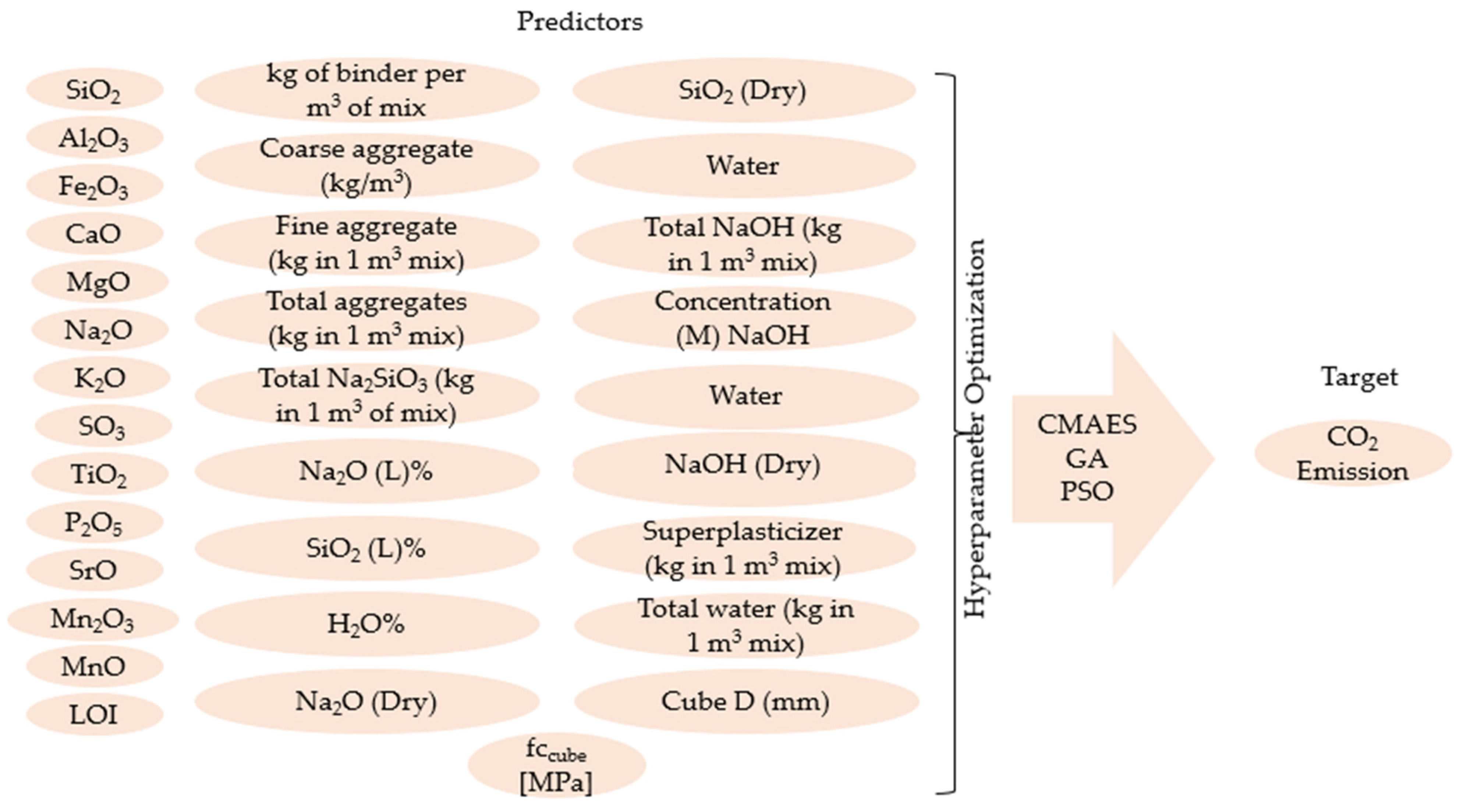
2.1. The Dataset

A comprehensive database of 1630 alkali-activated concrete samples was collected from the literature [36]. This database includes for each data sample the volumetric percentages of the main molecules in the concrete mix, the content and concentration of alkali activators, the water and superplasticizer amounts and the corresponding compressive strengths and carbon emissions. The statistical values of the predictors and target in the dataset used in CO2 prediction are given in Table 1. The Pearson correlation coefficients between different data features are shown in Figure 3 in a color-coded way. In Figure 3, a high linear correlation between the features is shown with the shades of blue, whereas inverse correlations are shown with the shades of red.

2.2. Using HyperNetExplorer

In this research, HyperNetExplorer developed by the writers was used. HyperNetExplorer is a web-based tool that aims to find an ANN architecture (model) that can be considered as the most accurate classification/regression (ML) model for a given dataset. HyperNetExplorer is a tool that depends on ANNs and uses various optimization algorithms from the MealPy [37] package for the hyperparameter optimization of the ANN. In this study, in order to determine the most efficient variable value, hyperparameter optimization was performed. Optimization algorithms such as “CMAES”, “GA” and “PSO” were used to perform hyperparameter optimization. The following sections provide information about ANN architectures, hyperparameter optimization algorithms, performance evaluation strategies and finally the HyperNetExplorer.

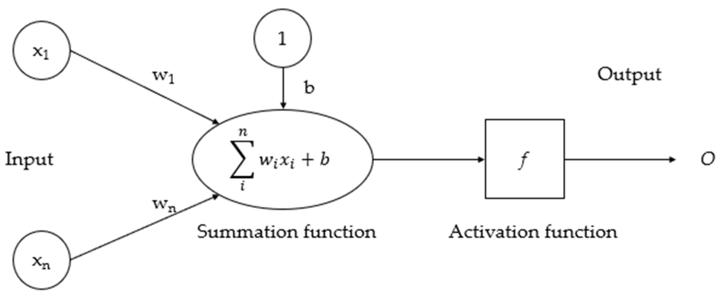
2.2.1. Artificial Neural Network (ANN)

The artificial neural network (ANN) can be defined as a computational method that tries to superficially simulate the neuron networks of the biological central nervous system [38]. ANN is superior to many traditional methods in that it is well adapted to all kinds of data that are difficult to define and difficult to obtain information about that can be inferred by experience or observation [39].
Here, each input is multiplied by its own weight, and all of these multiplications are summed. This sum is used to determine the activation level of the neural cell [40]. Artificial neural cells are also referred to as process elements in engineering science [41]. The coming together of neurons through connections with each other forms the artificial neural network given in Figure 4 [42].
In an artificial neural network, there are three layers. These layers are the input layer, output layer and hidden layer. The first layer is the input layer and allows external data to be received into the artificial neural network. The input layer consists of parameters that affect the problem. The number of neurons in the input layer is shaped according to the number of parameters. The hidden layer is between the input layer and the output layer. The neurons of the hidden layer have no connection with the external environment and only receive signals from the input layer and send signals to the output layer. The last layer, which is another layer of the model, is the output layer and provides the transmission of information to the outside [43].
Summation function: The summation function calculates the net input to the cell. Different functions are used for this function [44]. The weighted sum function is the most commonly used function and is expressed in Equation (1). Where G is the inputs, A is the weights, and N is the number of inputs.
N E T = i N G i A i
Activation function: The purpose of the activation function is to impart nonlinearity to the output of a neuron. In the studies, generally sigmoid, tanh and ReLU activation functions are used [45]. The activation functions in the hyperparameter optimization tool used in the study are shown in Figure 5.
The sigmoid activation function converts the input to a value between 0 and 1. Sigmoid is generally used for binary classification problems [45].
The tanh activation function converts the input to a value in the range [−1, 1] [45].
The Mish activation function represents a novel and non-monotonic approach compared to other functions. Experiments show that Mish tends to work better than ReLU in combination with other standard activation functions in many deep networks on challenging datasets [47].
The ReLU activation function brings nonlinearity to the network by equalizing negative values to zero and preserving positive values. In this way, it enables faster and more effective training. It is more effective in terms of performance than tanh and sigmoid functions that can be used instead of ReLU [45].
Leaky Relu leaking or leaking ReLU continues to minus infinity by definition. In other words, it is used for learning negative values in ReLU [48].
ELU (exponential linear unit): The exponential linear unit is similar to ReLU except for negative inputs. For negative inputs, parameter (a) is usually used [49].

2.2.2. Algorithms for Hyperparameter Optimization

Hyperparameters are parameters that differ according to the dataset and model used to generate a solution to a problem. The aim of hyperparameter optimization is to optimize the result obtained from the desired success criterion in any neural network model [50]. In this study, optimization algorithms such as “Covariance Matrix Adaptation Evolution Strategy (CMAES)”, “Genetic Algorithm (GA)” and “Particle Swarm Optimization (PSO)” were used to perform hyperparameter optimization.

CMAES (Covariance Matrix Adaptation Evolution Strategy)

The covariance matrix adaptation evolution strategy (CMAES) was introduced by Hansen and Ostermeier [51]. Evolutionary strategies (ESs) are stochastic, derivative-free methods for the numerical optimization of nonlinear optimization problems. The covariance matrix adaptation evolution strategy (CMA-ES) is a special type of strategy for numerical optimization [52].
The first step of the CMA-ES algorithm is parameter initialization. Population mutation is controlled using the mean value (mg), step size (σg) and covariance matrix (Cg) in Equation (2). In Equation (2), g is the population algebra.
x k g + 1 = m g + ϑ g N ( 0 , C g ) ,   k = 1 , . . . , λ
Offspring are selected according to the fitness function, and the first individuals with the lowest fitness value become the new generation population. The result is achieved when the set threshold condition is met [53].

Genetic Algorithm (GA)

The genetic algorithm (GA) was developed by John Holland [54] in the 1970s. The genetic algorithm (GA) is an optimization algorithm, often categorized as a global search heuristic technique. As a branch of evolutionary computation, it mimics the natural selection of biological reproduction processes and produces “optimal” solutions [55]. The algorithm consists of the stages of genetic coding for optimization applications, defining the goal, creating the initial population, selection operator, crossover operator, mutation, reaching the end criteria and showing the best result [56].
In genetic algorithms, the process begins with the random generation of the first generation. Evolutionary optimization is simulated by using genetic operators in all subsequent generations after the first randomly generated generation. Each individual in the population is represented by a chromosome and is one of the possible solutions to the problem. The objective function is used to calculate the solution quality (fitness) of chromosomes. Those with high fitness values are quality individuals. These individuals transmit the information in their genes to the next generation by breeding with individuals with high fitness values like themselves with the help of the crossover operator. With this method, genes from parents are transferred to children in different combinations, and new solutions are obtained. In order to avoid local minimum and maximum values, a certain amount of mutation operator (Equation (3)) is applied to change some of the genes in the chromosome in all generations. Finally, one of the situations occurs in which the new generation completely replaces the old, or the poor-quality individuals in the old generation are replaced by the quality individuals in the new generation. The iteration is continued until a satisfactory result is found [57].
X q , n e w = m r > r a n d ( ) ,   X q , m i n + r a n d ( )   ( X q , m a x X q , m i n )
In Equation (3), mr is mutation rate, q is a gene randomly selected from total design parameter, Xq,new is new values of qth parameter, Xq,min is lower limit value of qth parameter, and Xq,max is upper limit value of qth parameter. rand() is random number between 0 and 1.

Original Particle Swarm Optimization (PSO)

Particle swarm optimization (PSO) is a population-based heuristic optimization method proposed by Kennedy and Eberhart [58] in 1995 to describe the social behavior of birds and similar objects. PSO is based on the flock psychological behavior of flocks of birds or fish in search of food or traveling to a particular location. PSO is essentially based on bringing the position of the individuals in the herd closer to the individual with the best position in the herd. This approach speed is a randomly developing situation, and most of the time, individuals in the herd are in a better position than the previous position in their new movements, and this process continues until they reach the target [59].
In the particle swarm optimization algorithm, the initial swarm is first created with randomly generated initial positions and velocities. The fitness values of all particles in the swarm are calculated. For each particle, the local best (ybest) from the current generation is found. The number of the best in the herd is equal to the number of particles. The global best (gbest) is selected from the local best in the current generation. Position and velocities are restored using Equation (4) [59]. Equation (5) gives the new position value.
V i , n e w = w V i , j + c 1 r a n d ( ) ( X i , y b e s t X i , j ) + c 2 r a n d ( ) ( X i , g b e s t X i , j )
X i , n e w = X i , j + V i , n e w
In Equation (4), Xi,j gives position and Vi,j speed values, while rand() is a randomly generated number between 0 and 1. The steps from step 2 onward are repeated until the stopping criterion is met.

2.2.3. Performance Evaluation

Evaluating the success of models in machine learning is a very important stage. After the model is established, it is essential to evaluate its performance in order to make inferences about the model. In this study, the mean squared error (MSE) and R2 coefficient were used to evaluate and compare the results.
The mean squared error (MSE) is calculated from Equation (6) and is the mean of the squares of the errors. The error is the difference between the estimated value and the true value. MSE is a risk function corresponding to the expected value of the squared error loss [60]. The mean squared error is the average of the squares of the errors. Since the errors are squared, both the mean and standard deviation values are higher.
M S E = 1 n t = 1 n ( e t e t ) 2
In regression, the curve is fitted, and the other data are predicted based on the current numerical value. The coefficient of determination (R2) is a statistical measure of how close the data are to the fitted regression line. It is also known as the coefficient of determination or coefficient of multiple determination for multiple regression [61]. The formula of R2 is given in Equation (7).
  R 2 = 1 V a r i a n c e   t h a t   c a n   b e   e x p l a i n e d   b y   t h e   m o d e l T o t a l   v a r i a n c e

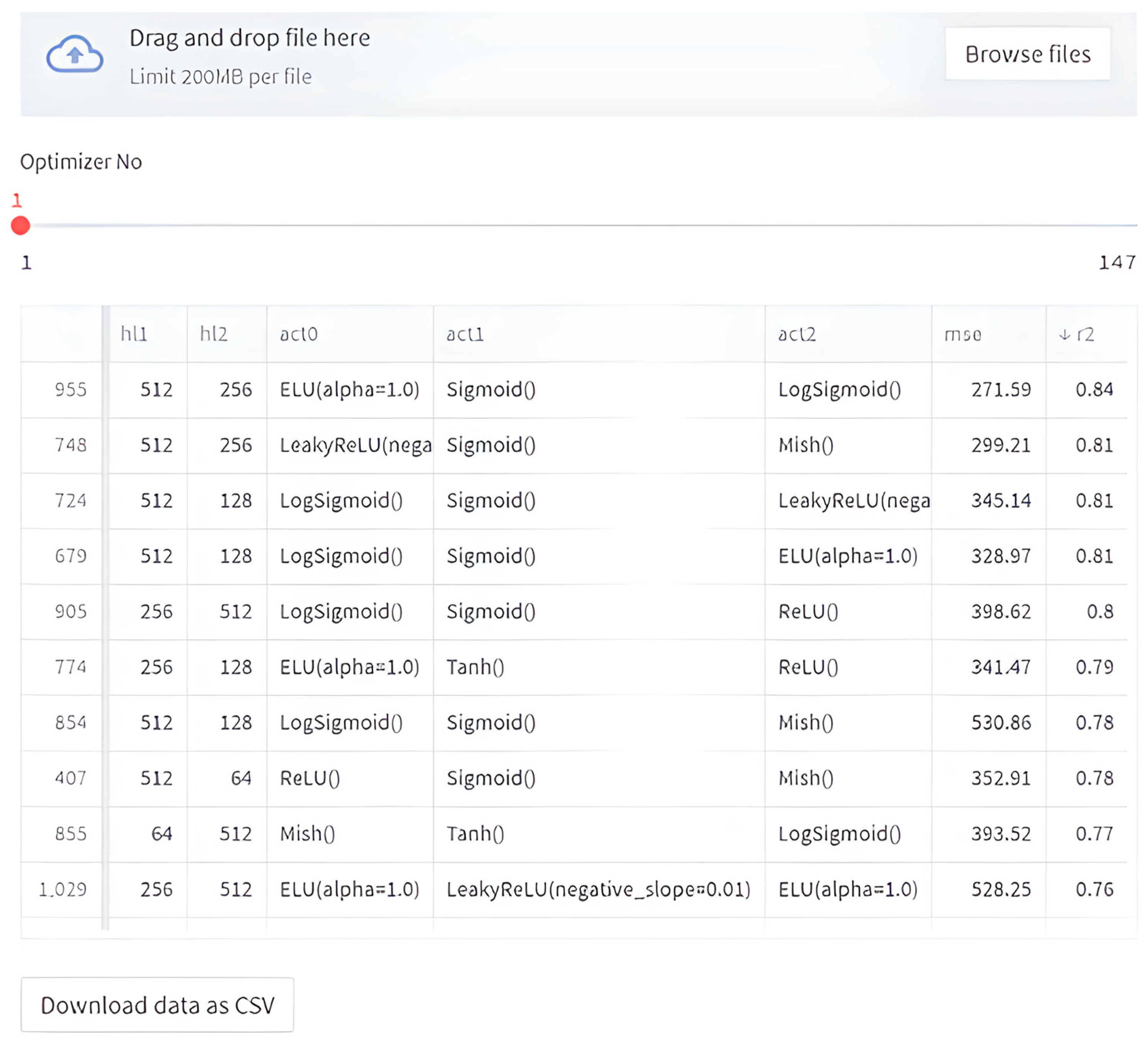
2.2.4. HyperNetExplorer: Architecture and Operation

The HyperNetExplorer depends on ANNs and utilizes several optimization algorithms from the MealPy [36] package for the hyperparameter optimization of the ANN. The tool is developed with Python and Pytorch [62] (as the ANN framework) and utilizes Streamlit as the GUI. The parameters to be optimized and their ranges are listed in Table 2.
In the default configuration of the tool, the learning rate is set to 0.001 and the number of epochs to 200. CrossEntropyLoss is used as the loss function for classification and MSELoss for regression-type problems. The tool can use all the optimization algorithms provided by the MealPy package. In the current configuration of the tool used for this dataset, MealPy’s CMAES, GA and PSO algorithms were used to optimize the hyperparameters. A graphical user interface (GUI) is used when loading the dataset into the system. When the FindBestNet command is issued through the GUI after the dataset is loaded, the objective function of the tool builds an ANN based on a set of hyperparameters provided by the user at each iteration of the optimizer. Once an ANN is generated, the accuracy of this ANN is calculated through 10-fold cross-validation. The output of the objective function is the average of the measures of these 10 folds. This output is consumed/evaluated by the optimizer, and based on this, the objective function is called again with a new set of hyperparameters. The default parameters for the optimizer are 20 epochs and a population size of 50; this creates at least 20 × 50 = 1000 ANN architectures in each run. For each generated network, parameter values, mean squared error (MSE) and coefficient of determination (R2) are provided as a table in the Streamlit-based GUI. Once training is complete, all ANN models are stored on the server and can be downloaded as (*.pt) files.

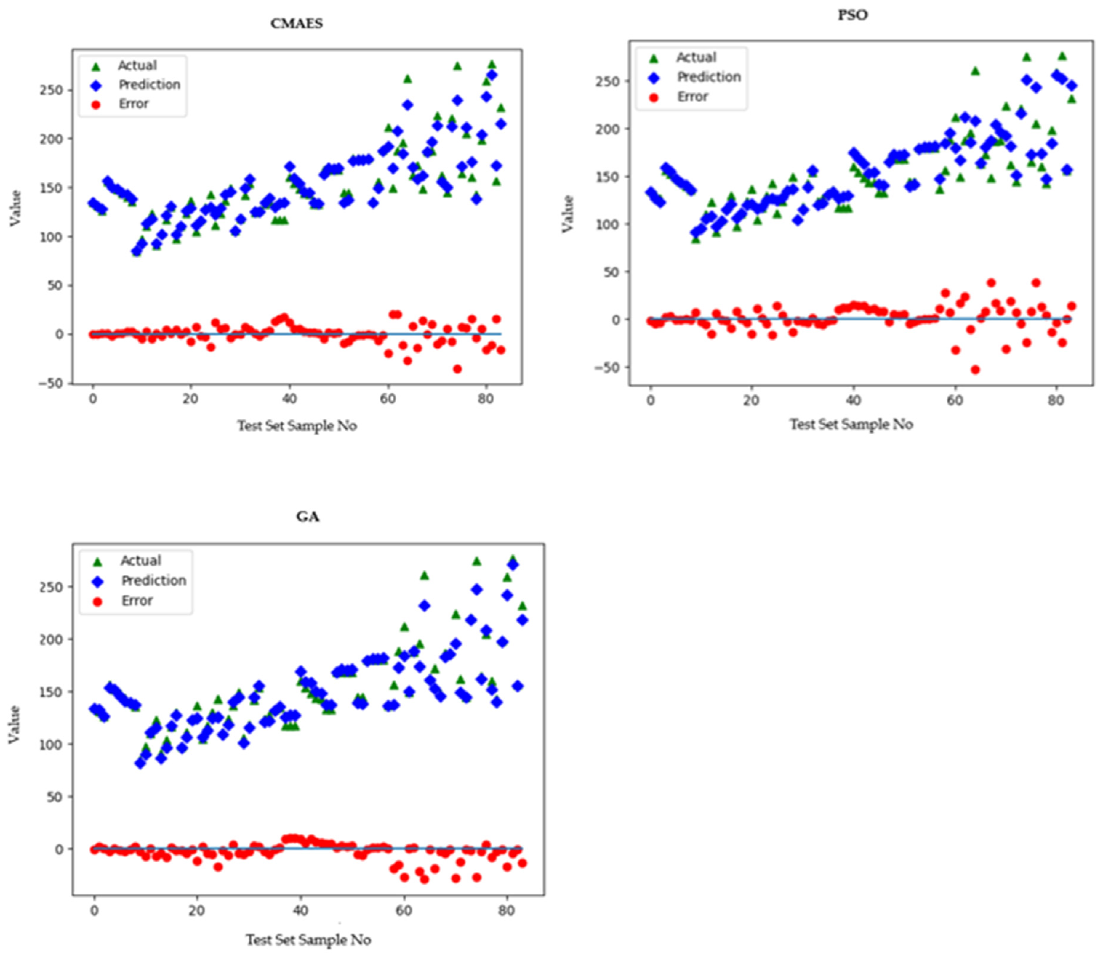
3. Results and Discussion

In this study, as mentioned before, three optimizers (CMAES, GA and PSO) for CO2 prediction from the MealPy [37] package were tested. HyperNetExplorer managed to discover ANN architectures for the CO2 dataset. The general scheme of the study is shown in Figure 6.
Figure 7 shows HyperNetExplorer’s web-based user interface showing in descending order the metadata of the 10 best-performing ANNs discovered with the covariance matrix adaptation evolution strategy (CMAES). The MSE range of the 10 best-performing ANN architectures is 187.07–231.68. The R2 range of the 10 best-performing ANN architectures is 0.85–0.88.
The performance shown by CMAES and the metadata regarding the architecture of the ANN are given in Table 3.
Figure 8 shows HyperNetExplorer’s web-based user interface showing in descending order the metadata of the 10 best-performing ANNs discovered with the genetic algorithm (GA). The MSE range of the 10 best-performing ANN architectures is 161.17–182.07. The R2 range of the 10 best-performing ANN architectures is 0.89–0.9.
The performance shown by the GA and the metadata regarding the architecture of the ANN are given in Table 4.
Figure 9 shows HyperNetExplorer’s web-based user interface showing in descending order the metadata of the 10 best-performing ANNs discovered with particle swarm optimization (PSO). The MSE range of the 10 best-performing ANN architectures is 271.59–528.25. The R2 range of the 10 best-performing ANN architectures is 0.76–0.984.
The performance shown by PSO and the metadata regarding the architecture of the ANN are given in Table 5.
Figure 10 shows the scatter plots of the relationship between two different variables obtained with each optimization algorithm used. As can be seen from Figure 8, the genetic algorithm (GA), which has the highest R2 value, has the lowest error rate. The highest error rate is in particle swarm optimization (PSO). A low error rate means that the actual value and predicted values are close to each other. This shows that the prediction model is effective in terms of success and reliability. The higher the error rate, the further away it is from the prediction that is considered correct. As can be seen in Figure 10, the smallest difference between the actual and predicted value is in the GA while the biggest difference is in PSO.
Table 6 shows the best accuracy rates achieved by the explored ANN architectures for the CO2 dataset using CMAES, GA and PSO optimizers. The best MSE and R2 achieved for each optimizer is given in Table 6.
When Table 6 is examined, it is seen that the algorithm with the lowest mean squared error (MSE) and the highest coefficient of determination (R2) with hyperparameter optimization is the genetic algorithm (GA). The result obtained with the GA is better than the mean squared error and coefficient of determination obtained after regression analysis with hyperparameter optimization with covariance matrix adaptation evolution strategy (CMAES) and particle swarm optimization (PSO). After the GA, CMAES (MSE = 187.07 and R2 = 0.88) showed the best performance. PSO (MSE = 271.59 and R2 = 0.84) showed the lowest performance.
When the number of iterations in which the algorithms find the best among themselves, i.e., their speed, is compared, it is seen that CMAES is the fastest algorithm with 699 iterations. A radar chart of the prediction accuracies and speed of convergence is shown in Figure 11.

4. Conclusions

The amount of carbon dioxide emitted into the atmosphere is rapidly increasing. As the increase in the amount of carbon dioxide continues, the global warming problem will grow further. For this reason, researchers have begun to investigate methods to reduce the amount of carbon dioxide. Thanks to correctly used data, resources can be controlled efficiently. The use of alkali-activated binders instead of ordinary Portland cement (OPC) will bring great advantages in both environmental and economic terms and will contribute to the production of sustainable materials. However, the carbon emissions and mechanical properties of alkali-activated concrete can widely fluctuate depending on the chemical composition of the concrete mix. Therefore, machine learning that enables the accurate prediction of these properties based on the chemical ingredients of alkali-activated concrete is necessary for the widespread adoption of this construction material. Artificial neural networks (ANNs) are one of the machine learning methods that use data and have been widely used in data analysis in recent years. Artificial neural networks perform better than other classical statistical methods and provide successful results. In this study, alkali-activated binders were proposed as an alternative to reduce the environmental impact of ordinary Portland cement production.
The results indicate that the carbon emission associated with alkali-activated concrete production can be predicted with high accuracy using state-of-the-art machine learning techniques. In this study, three different hyperparameter optimization algorithms (covariance matrix adaptation evolution strategy (CMAES), genetic algorithm (GA) and particle swarm optimization (PSO)) were compared and evaluated according to performance metrics (mean squared error (MSE) and coefficient of determination (R2)) for a CO2 prediction dataset.
The results of the hyperparameter optimization can be summarized as follows:
(1)
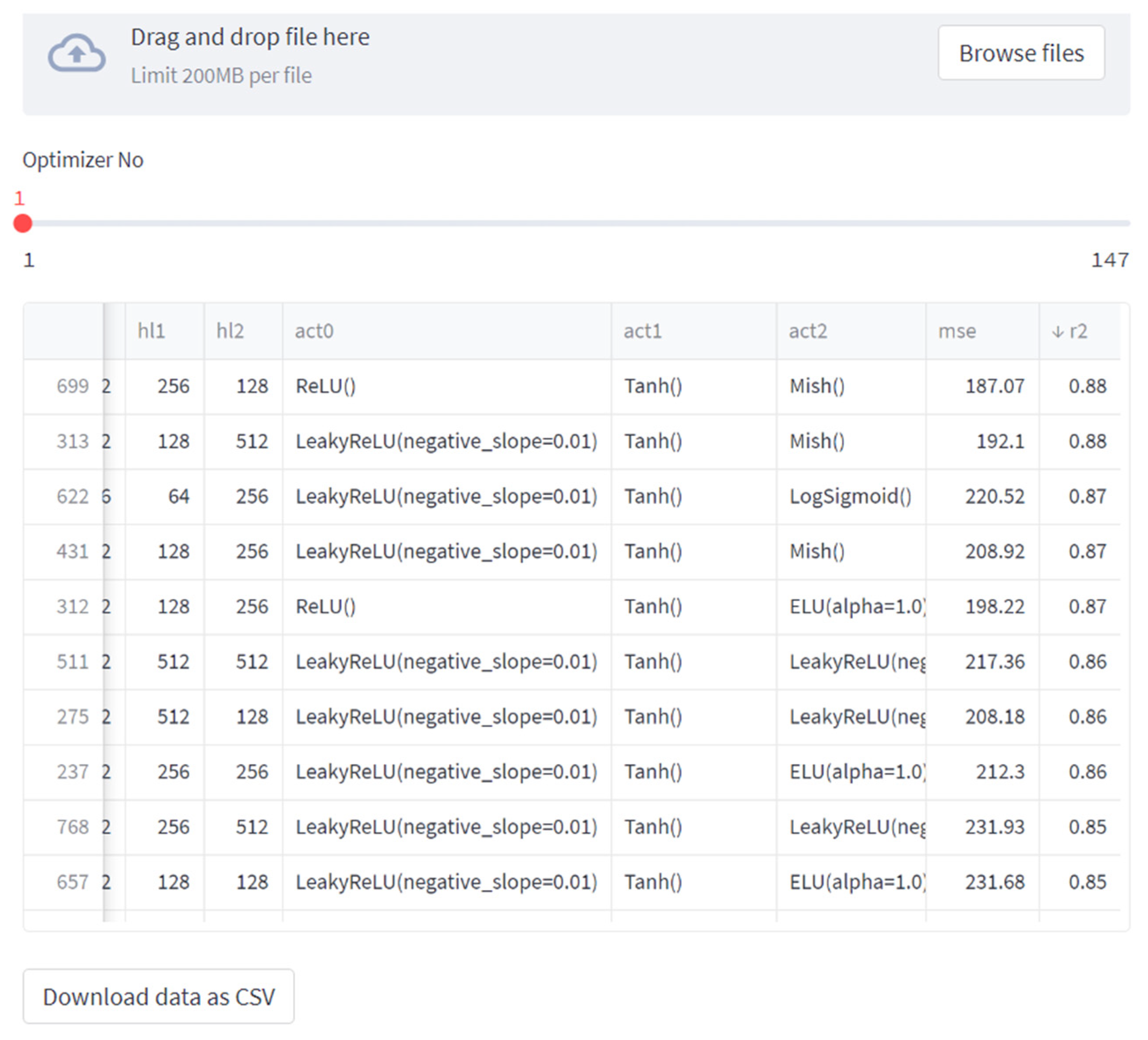
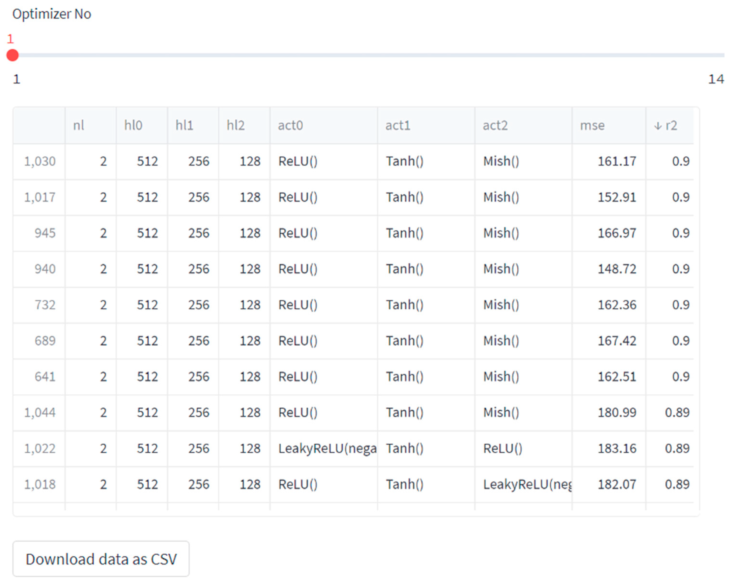
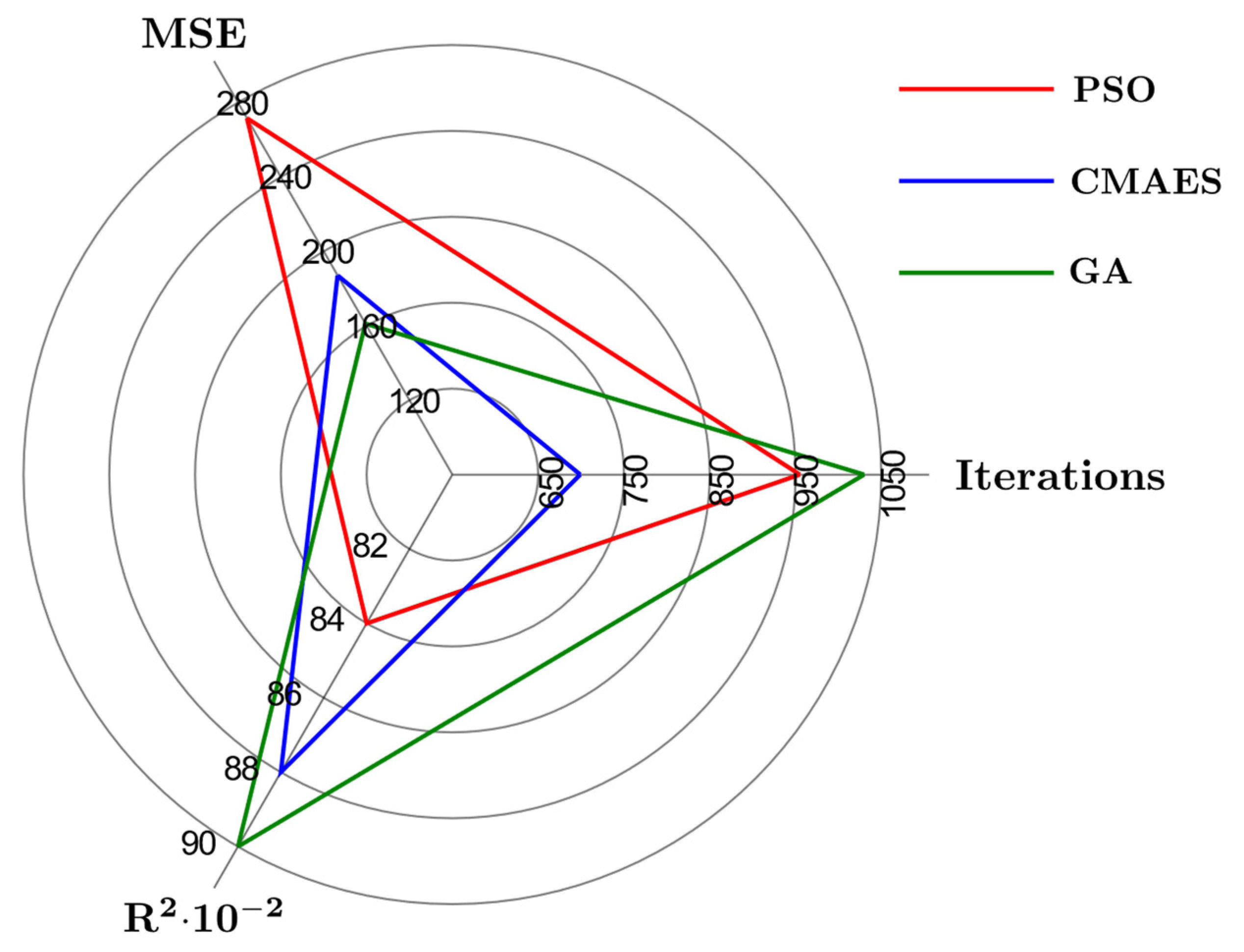
Hyperparameter optimization with the genetic algorithm showed successful regression performance with accurate mean squared error (MSE = 161.17) and coefficient of determination (R2 = 0.90) values in the datasets.
(2)
CMAES follows the GA with MSE = 187.07 and R2 = 0.88.
(3)
The algorithm with the lowest R2 (R2 = 0.84) value and the highest MSE (MSE = 271.59) among them is PSO.
These results show that the hyperparameter optimization algorithm can achieve good accuracy for the prediction of CO2 emission associated with alkali-activated concrete production. This study contributes to the production of environmentally friendly and sustainable binder materials with very low CO2 emissions and production energy that can be used as ordinary Portland cement (OPC) substitutes.

Author Contributions

Y.A. and Ü.I. generated the analysis codes; Y.A., Ü.I. and G.B. developed the theory, background and formulations of the problem; verification of the results was performed by Y.A., Ü.I., G.B. and C.C.; the text of the paper was written by Y.A., Ü.I., G.B. and C.C.; the text of the paper was edited by G.B., S.K., J.H. and Z.W.G.; the figures were drawn by Y.A.; G.B. and Z.W.G. supervised the research direction; J.H. and Z.W.G. acquired funding. All authors have read and agreed to the published version of the manuscript.

Funding

This work was supported by the Korea Institute of Energy Technology Evaluation and Planning (KETEP) and the Ministry of Trade, Industry Energy (MOTIE) of the Republic of Korea (No. 20192010106990). This work was also supported by the Gachon University research fund of 2023 (GCU-202303680001).

Institutional Review Board Statement

Not applicable.

Informed Consent Statement

Not applicable.

Data Availability Statement

Data are available on request to authors.

Conflicts of Interest

The authors declare no conflicts of interest.

References

  1. İğci, T.; Çobanoğlu, N. An Assessment of Climate Change and Global Agreements from the Perspective of Environmental Ethics. Ank. Univ. J. Environ. Sci. 2019, 7, 130–146. [Google Scholar]
  2. Aksan, Z.; Çelikler, D. Pre-Service Elementary Teachers’ Opinions about Global Warming. Eskişehir Osman. Univ. J. Soc. Sci. 2013, 14, 49–67. [Google Scholar]
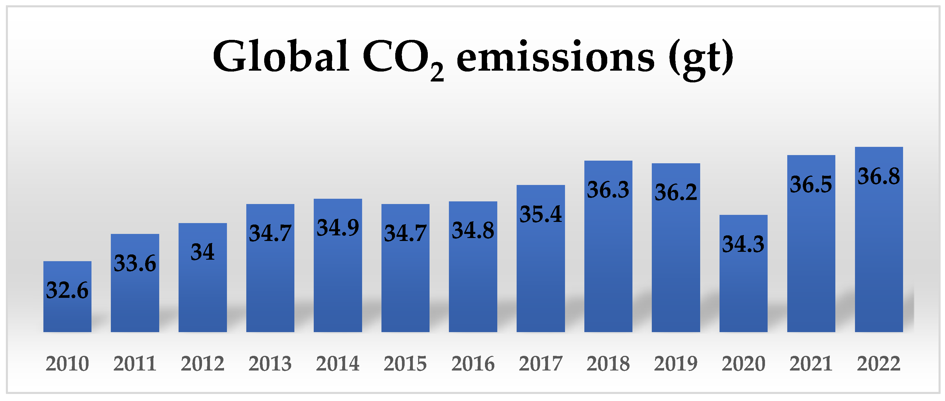
  3. CO2 Emissions in 2022. Available online: https://www.iea.org/reports/co2-emissions-in-2022 (accessed on 20 September 2023).
  4. Mehta, K.P. Reducing the environmental impact of concrete. Concr. Int. 2001, 23, 61–66. [Google Scholar]
  5. United Nations Development. Sustainable Development Goals. 2015. Available online: https://www.undp.org/susabinable-development-goals (accessed on 20 September 2023).
  6. Erdoğan, T.Y. Concrete, Turkey; Hermes Promotion Offset Printing Services, Ltd.: Ottawa, ON, Canada, 2013. [Google Scholar]
  7. Kawashima, A.B.; Martins, L.D.; Rafee, S.A.A.; Rudke, A.P.; de Morais, M.V.; Martins, J.A. Development of a spatialized atmospheric emission inventory for the main industrial sources in Brazil. Environ. Sci. Pollut. Res. 2020, 27, 35941–35951. [Google Scholar] [CrossRef] [PubMed]
  8. Uzal, B.; Turanli, L.; Mehta, P.K. High-volume natural pozzolan concrete for structural applications. ACI Mater. J. 2007, 104, 535. [Google Scholar]
  9. About Cement & Concrete. Available online: https://gccassociation.org/our-story-cement-and-concrete/ (accessed on 20 September 2023).
  10. Cement: The Hidden Culprit of Global Warming. Available online: https://www.bbc.com/turkce/haberler-dunya-46589916 (accessed on 20 September 2023).
  11. CMIE. Infomerics Economic Research. Available online: https://www.infomerics.com/admin/uploads/Cement-Industry-Report-May2023.pdf (accessed on 21 September 2023).
  12. Wu, H.; Hu, R.; Yang, D.; Ma, Z. Micro-macro characterizations of mortar containing construction waste fines as replacement of cement and sand: A comparative study. Constr. Build. Mater. 2023, 383, 131328. [Google Scholar] [CrossRef]
  13. Dobiszewska, M.; Bagcal, O.; Beycioğlu, A.; Goulias, D.; Köksal, F.; Płomiński, B.; Ürünveren, H. Utilization of rock dust as cement replacement in cement composites: An alternative approach to sustainable mortar and concrete productions. J. Build. Eng. 2023, 69, 106180. [Google Scholar] [CrossRef]
  14. Moumin, G.; Ryssel, M.; Zhao, L.; Markewitz, P.; Sattler, C.; Robinius, M.; Stolten, D. CO2 emission reduction in the cement industry by using a solar calciner. Renew. Energy 2020, 145, 1578–1596. [Google Scholar] [CrossRef]
  15. Chaudhury, R.; Sharma, U.; Thapliyal, P.C.; Singh, L.P. Low-CO2 emission strategies to achieve net zero target in cement sector. J. Clean. Prod. 2023, 417, 137466. [Google Scholar]
  16. Cakiroglu, C.; Islam, K.; Bekdas, G.; Apak, S. Cost and CO2 emission-based optimisation of reinforced concrete deep beams using Jaya algorithm. J. Environ. Prot. Ecol. 2022, 23, 9534. [Google Scholar]
  17. Cakiroglu, C.; Islam, K.; Bekdaş, G.; Billah, M. CO2 emission and cost optimization of concrete-filled steel tubular (CFST) columns using metaheuristic algorithms. Sustainability 2021, 13, 8092. [Google Scholar] [CrossRef]
  18. Artel, T. Building Materials, 2nd ed.; Gündüz, D., Ed.; Osman Yalçın Printing House: Istanbul, Turkey, 1969. [Google Scholar]
  19. Buchwald, A.; Kaps, C.; Hohmann, M. Alkali-activated binders and pozzolan cement binders–complete binder reaction or two sides of the same story. In Proceedings of the 11th International Congress on the Chemistry of Cement (ICCC), Durban, South Africa, 11–16 May 2003; pp. 1238–1246. [Google Scholar]
  20. Shi, C.; Krivenko, P.V.; Roy, D.M. Alkali-Activated Cements and Concretes; Taylor and Francis: Abingdon, UK, 2006. [Google Scholar]
  21. Pacheco-Torgal, F.; Castro-Gomes, J.; Jalali, S. Alkali-activated binders: A review: Part 1. Historical background, terminology, reaction mechanisms and hydration products. Constr. Build. Mater. 2008, 22, 1305–1314. [Google Scholar] [CrossRef]
  22. Provis, J.L.; Van Deventer, J.S. Alkali Activated Materials: State-of-the-Art Report, RILEM TC 224-AAM; Provis, J.L., Van Deventer, J.S., Eds.; Springer Science & Business Media: Berlin/Heidelberg, Germany, 2013; Volume 13. [Google Scholar]
  23. Hamrani, A.; Akbarzadeh, A.; Madramootoo, C.A. Machine learning for predicting greenhouse gas emissions from agricultural soils. Sci. Total Environ. 2020, 741, 140338. [Google Scholar] [CrossRef] [PubMed]
  24. Leerbeck, K.; Bacher, P.; Junker, R.G.; Goranović, G.; Corradi, O.; Ebrahimy, R.; Tveit, A.; Madsen, H. Short-term forecasting of CO2 emission intensity in power grids by machine learning. Appl. Energy 2020, 277, 115527. [Google Scholar] [CrossRef]
  25. Li, Y.; Sun, Y. Modeling and predicting city-level CO2 emissions using open access data and machine learning. Environ. Sci. Pollut. Res. 2021, 28, 19260–19271. [Google Scholar] [CrossRef] [PubMed]
  26. Li, X.; Ren, A.; Li, Q. Exploring patterns of transportation-related CO2 emissions using machine learning methods. Sustainability 2022, 14, 4588. [Google Scholar] [CrossRef]
  27. Wang, C.; Li, M.; Yan, J. Forecasting carbon dioxide emissions: Application of a novel two-stage procedure based on machine learning models. J. Water Clim. Change 2023, 14, 477–493. [Google Scholar] [CrossRef]
  28. He, B.; Zhu, X.; Cang, Z.; Liu, Y.; Lei, Y.; Chen, Z.; Wang, Y.; Zheng, Y.; Cang, D.; Zhang, L. Interpretation and Prediction of the CO2 Sequestration of Steel Slag by Machine Learning. Environ. Sci. Technol. 2023, 57, 17940–17949. [Google Scholar] [CrossRef]
  29. Amin, M.N.; Ahmad, W.; Khan, K.; Al-Hashem, M.N.; Deifalla, A.F.; Ahmad, A. Testing and modeling methods to experiment the flexural performance of cement mortar modified with eggshell powder. Case Stud. Constr. Mater. 2023, 18, e01759. [Google Scholar] [CrossRef]
  30. Wang, P.; Hu, J.; Chen, W. A hybrid machine learning model to optimize thermal comfort and carbon emissions of large-space public buildings. J. Clean. Prod. 2023, 400, 136538. [Google Scholar] [CrossRef]
  31. Yücel, M.; Bekdaş, G.; Nigdeli, S.M. Prediction of Minimum CO2 Emission for Rectangular Shape Reinforced Concrete (RC) Beam. In Proceedings of the 7th International Conference on Harmony Search, Soft Computing and Applications, ICHSA, Seoul, Republic of Korea, 3 September 2022; Springer Nature: Singapore, 2022; pp. 139–148. [Google Scholar]
  32. Bekdaş, G.; Yucel, M.; Nigdeli, S.M. Generation of eco-friendly design for post-tensioned axially symmetric reinforced concrete cylindrical walls by minimizing of CO2 emission. Struct. Des. Tall Spec. Build. 2022, 31, e1948. [Google Scholar] [CrossRef]
  33. Aydın, Y.; Bekdaş, G.; Nigdeli, S.M.; Isıkdağ, Ü.; Kim, S.; Geem, Z.W. Machine learning models for ecofriendly optimum design of reinforced concrete columns. Appl. Sci. 2023, 13, 4117. [Google Scholar] [CrossRef]
  34. Sun, Y.; Cheng, H.; Zhang, S.; Mohan, M.K.; Ye, G.; De Schutter, G. Prediction & optimization of alkali-activated concrete based on the random forest machine learning algorithm. Constr. Build. Mater. 2023, 385, 131519. [Google Scholar]
  35. Cakiroglu, C.; Bekdaş, G. CO2 Emission Minimization of a Plate Girder under Lateral Torsional Buckling Constraint. In AIP Conference Proceedings; AIP Publishing: Long Island, NY, USA, 2023; Volume 2849. [Google Scholar]
  36. Torres, B.M.; Völker, C.; Firdous, R. An Alkali-Activated Concrete Dataset for Sustainable Building Materials. Zenodo 2023, 2, 7805018. [Google Scholar] [CrossRef]
  37. Mealpy. Available online: https://github.com/thieu1995/mealpy (accessed on 23 September 2023).
  38. Kohonen, T. An introduction to neural computing. Neural Netw. 1988, 1, 3–16. [Google Scholar] [CrossRef]
  39. Zhang, G.; Patuwo, B.E.; Hu, M.Y. Forecasting with artificial neural networks: The state of the art. Int. J. Forecast. 1998, 14, 35–62. [Google Scholar] [CrossRef]
  40. Akkaya, G. Artificial Neural Networks and Their Applications in Agriculture. J. Atatürk Univ. Fac. Agric. 2007, 38, 195–202. [Google Scholar]
  41. Oztemel, E. Artificial Neural Networks; Papatya Publishing: Istanbul, Turkey, 2006. [Google Scholar]
  42. Kurt, R.; Karayilmazlar, S.; Imren, E.; Çabuk, Y. Forecasting by Using Artificial Neural Networks: Turkey’s Paper Paperboard Industry Case. J. Bartin Fac. For. 2017, 19, 99–106. [Google Scholar]
  43. Benli, Y. The Use of Artificial Neural Network in the Prediction of Financial Failure and an Application in ISE. J. Account. Sci. World 2002, 4, 17–30. [Google Scholar]
  44. Alaloul, W.S.; Qureshi, A.H. Data Processing Using Artificial Neural Networks; IntechOpen: London, UK, 2020. [Google Scholar] [CrossRef]
  45. Şafak, E. Detection of fake face images using convolutional neural networks. Master’s Thesis, Gazi University, Ankara, Turkey, 2023. [Google Scholar]
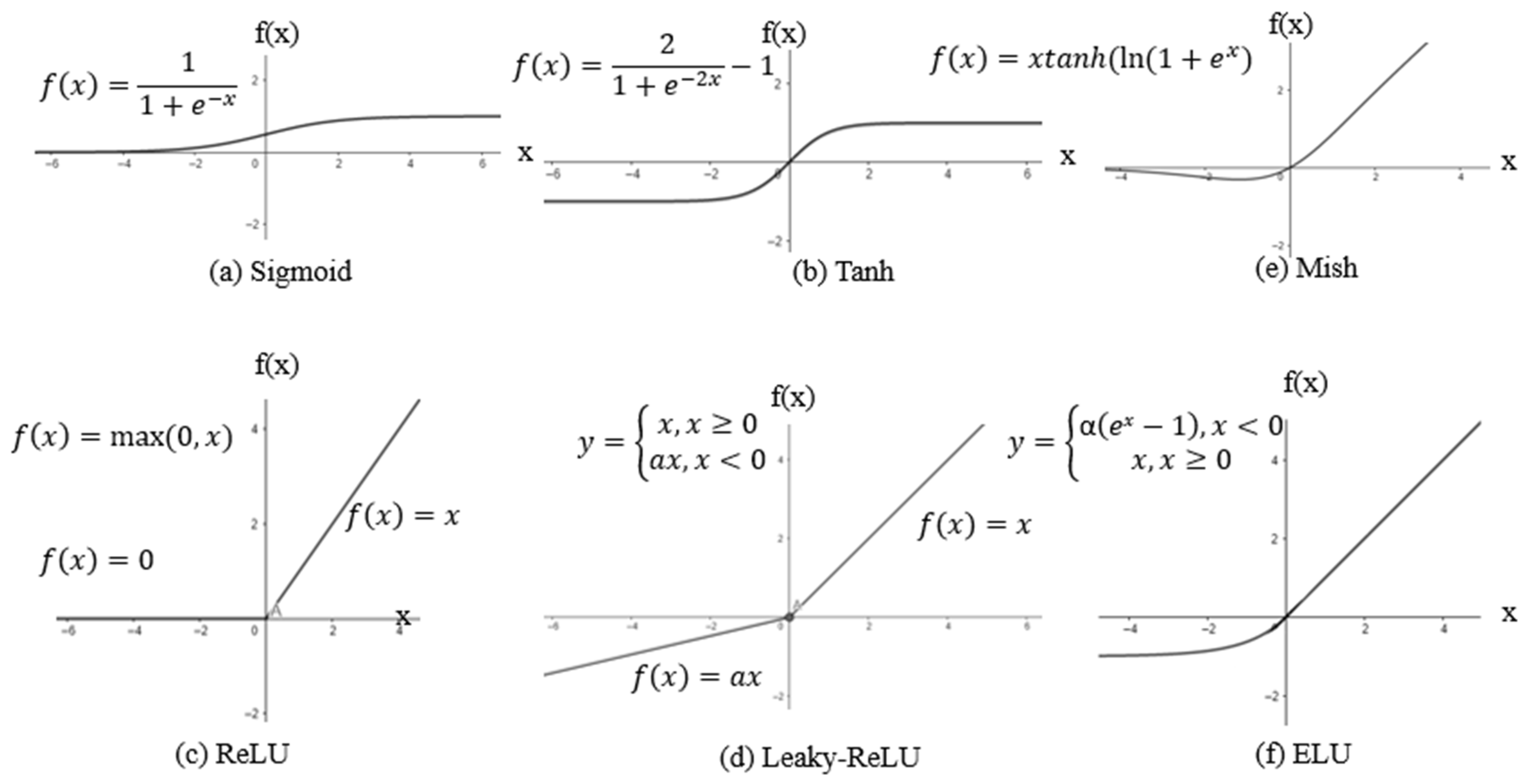
  46. Karlik, B.; Olgac, A.V. Performance analysis of various activation functions in generalized MLP architectures of neural networks. Int. J. Artif. Intell. Expert Syst. 2011, 1, 111–122. [Google Scholar]
  47. Misra, D. Mish: A Self Regularized Non-monotonic Activation Function. arXiv 2019, arXiv:1908.08681. [Google Scholar]
  48. Xu, J.; Li, Z.; Du, B.; Zhang, M.; Liu, J. Reluplex made more practical: Leaky ReLU. In Proceedings of the 2020 IEEE Symposium on Computers and Communications (ISCC), Rennes, France, 7 July 2020; pp. 1–7. [Google Scholar] [CrossRef]
  49. Clevert, D.A.; Unterthiner, T.; Hochreiter, S. Fast and accurate deep network learning by exponential linear units (elus). arXiv 2015, arXiv:1511.07289. [Google Scholar]
  50. Atlan, F.; Hançer, E.; Pençe, İ. Evaluation of Hyper Parameter Optimization Effect on Nuclei Segmentation with U-Net. Eur. J. Sci. Technol. 2020, 22, 60–69. [Google Scholar]
  51. Hansen, N.; Ostermeier, A. Adapting arbitrary normal mutation distributions in evolution strategies: The covariance matrix adaptation. In Proceedings of the IEEE International Conference on Evolutionary Computation, Nagoya, Japan, 20–22 May 1996; pp. 312–317. [Google Scholar]
  52. CMA-ES. Available online: https://en.wikipedia.org/wiki/CMA-ES (accessed on 25 September 2023).
  53. Chen, G.; Yin, J.; Yang, S. Ship Autonomous Berthing Simulation Based on Covariance Matrix Adaptation Evolution Strategy. J. Mar. Sci. Eng. 2023, 11, 1400. [Google Scholar] [CrossRef]
  54. Holland, J.H. Genetic algorithms and the optimal allocation of trials. SIAM J. Comput. 1973, 2, 88–105. [Google Scholar] [CrossRef]
  55. Okwu, M.O.; Tartibu, L.K. Metaheuristic Optimization: Nature-Inspired Algorithms Swarm and Computational Intelligence, Theory and Applications; Springer Nature: Singapore, 2020; Volume 927. [Google Scholar]
  56. Keklik, G.; Özcan, B.D. Functioning of Genetic Algorithms and Operators Used in Genetic Algorithm Applications. Osman. Korkut Ata Univ. J. Inst. Sci. Technol. 2023, 6, 1052–1066. [Google Scholar]
  57. Az, M.T.; Ayvaz, B. Genetic Algorithm Application for Crew Pair Optimization in Airline Crew Planning. Istanb. Commer. Univ. J. Sci. 2022, 21, 194–210. [Google Scholar]
  58. Eberhart, R.; Kennedy, J. Particle swarm optimization. In Proceedings of the IEEE International Conference on Neural Networks, Perth, WA, Australia, 27 November–1 December 1995; Volume 4, pp. 1942–1948. [Google Scholar]
  59. Özsağlam, M.Y.; Çunkaş, M. Particle Swarm Optimization Algorithm for Solving Optimızation Problems. J. Polytech. 2008, 11, 299–305. [Google Scholar]
  60. Zhu, W.; Yao, T.; Ni, J.; Wei, B.; Lu, Z. Dependency-based Siamese long short-term memory network for learning sentence representations. PLoS ONE 2018, 13, e0193919. [Google Scholar] [CrossRef]
  61. Evaluating Model Performance—Metrics. Available online: https://medium.com/deep-learning-turkiye/model-performans%C4%B1n%C4%B1-de%C4%9Ferlendirmek-metrikler-cb6568705b1 (accessed on 2 October 2023).
  62. Paszke, A.; Gross, S.; Massa, F.; Lerer, A.; Bradbury, J.; Chanan, G.; Killeen, T.; Lin, Z.; Gimelshein, N.; Antiga, L.; et al. Pytorch: An imperative style, high-performance deep learning library. arXiv 2019, arXiv:1912.01703. [Google Scholar]
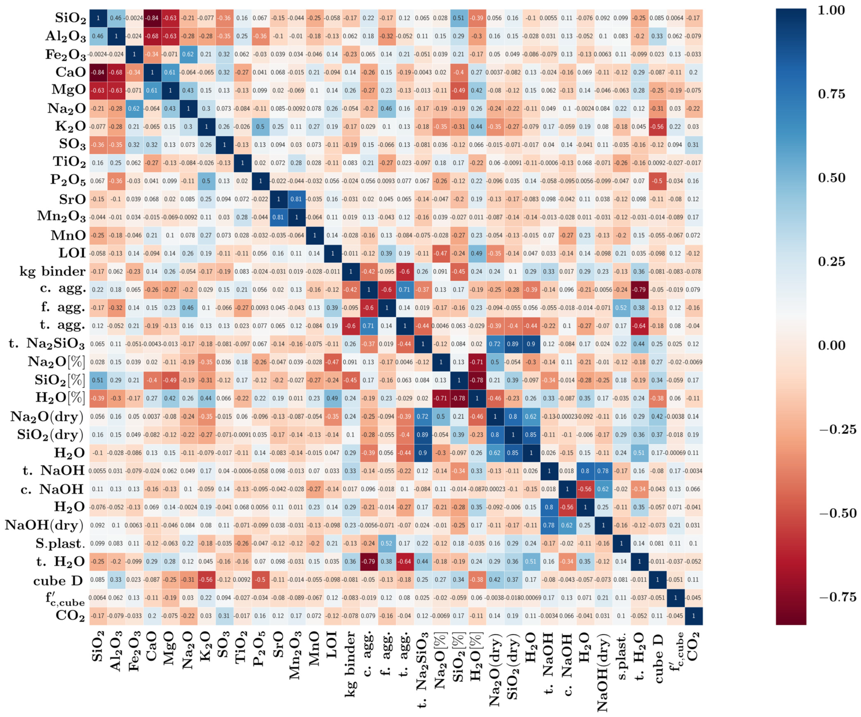
Figure 1. Global CO2 emissions from energy combustion and industrial processes [3].
Sustainability 16 00142 g001
Figure 2. Production of cement in India by year [11].
Sustainability 16 00142 g002
Figure 3. Correlation heat map.
Sustainability 16 00142 g003
Figure 4. Artificial neural networks consisting of artificial nerve cells [42].
Sustainability 16 00142 g004
Figure 5. Activation functions [46].
Sustainability 16 00142 g005
Figure 6. Predictors and target of the hyperparameter optimization process.
Sustainability 16 00142 g006
Figure 7. Ten best-performing ANNs discovered by CMAES optimizer.
Sustainability 16 00142 g007
Figure 8. Ten best-performing ANNs discovered by GA optimizer.
Sustainability 16 00142 g008
Figure 9. Ten best-performing ANNs discovered by PSO optimizer.
Sustainability 16 00142 g009
Figure 10. Scatter plots for each optimization algorithm.
Sustainability 16 00142 g010
Figure 11. Optimizer performances.
Sustainability 16 00142 g011
Table 1. Predictors and target of the dataset and their statistical values.
PredictorMin–Max
Value
MeanStandard
Deviation
SiO230.61–77.150.1669.377
Al2O34.26–38.3823.3656.710
Fe2O30.3–17.864.4652.888
CaO0.05–43.3412.99311.802
MgO0–9.573.0282.629
Na2O0–3.660.4340.552
K2O0–5.030.8771.111
SO30–5.040.6760.793
TiO20–2.190.5600.723
P2O50–4.480.2000.655
SrO0–0.50.0010.007
Mn2O30–0.290.0100.039
MnO0–0.370.0120.050
LOI0–13.971.2541.474
kg of binder per m3 of mix150–788.58402.93888.017
Coarse aggregate (kg/m3)525.4–1591.341093.954181.134
Fine aggregate (kg in 1 m3 mix)318.27669.847122.338
Total aggregates (kg in 1 m3 mix)11101763.798150.755
Total Na2SiO3 (kg in 1 m3 of mix)49.6–213123.88731.492
Na2O (L)%0.08–0.230.1390.027
SiO2 (L)%0.21–0.350.3030.031
H2O%0.48–0.640.5580.046
Na2O (Dry)6.08–35.1816.8435.280
SiO2 (Dry)11.23–66.8437.16210.947
Water25.26–130.5167.96719.300
Total NaOH (kg in 1 m3 mix)22.5–133.1859.07817.977
Concentration (M) NaOH3–2210.9273.112
Water8.51–79.9133.21712.243
NaOH (Dry)2.98–85.2425.86111.628
Superplasticizer (kg in 1 m3 mix)0–475.8387.246
Total water (in solutions + additional)
(kg in 1 m3 mix)
41.38–303.54124.05349.615
Cube D (mm)50–150121.26727.337
fccube (MPa)3–91.9445.55415.256
Target
CO2 footprint
(kg emision per 1 m3 of samples)
38.23–895.07154.47386.962
Table 2. Parameters to be optimized.
Parameter NameLower BoundUpper BoundOptions
Number of Hidden Layers (HLs)020: Single HL
1: Two HL
2: Three HL
Number of Neurons in HL = 1060: 8
1: 16
2: 32
3: 64
4: 128
5: 256
6: 512
Number of Neurons in HL = 2060: 8
1: 16
2: 32
3: 64
4: 128
5: 256
6: 512
Number of Neurons in HL = 3060: 8
1: 16
2: 32
3: 64
4: 128
5: 256
6: 512
Activation Function of HL = 1060: LeakyReLU
1: Sigmoid
2: Tanh
3: ReLU
4: LogSigmoid
5: ELU
6: Mish
Activation Function of HL = 2060: LeakyReLU
1: Sigmoid
2: Tanh
3: ReLU
4: LogSigmoid
5: ELU
6: Mish
Activation Function of HL = 3060: LeakyReLU
1: Sigmoid
2: Tanh
3: ReLU
4: LogSigmoid
5: ELU
6: Mish
Table 3. CO2 dataset neural network structure and parameters (CMAES).
Neural Network StructureParameters
Type of optimization methodCMAES
Number of layers in the network5
Number of neurons in the input layer33
Number of hidden layers3
Number of hidden layer neurons512-256-128
Total number of iterations1050
Number of best iteration699
Mean squared error (MSE)187.07
Coefficient of determination (R2)0.88
Table 4. CO2 dataset neural network structure and parameters (GA).
Neural Network StructureParameters
Type of optimization methodGenetic Algorithm
Number of layers in the network5
Number of neurons in the input layer33
Number of hidden layers3
Number of hidden layer neurons512-256-128
Total number of iterations1050
Number of best iteration1030
Mean squared error (MSE)161.17
Coefficient of determination (R2)0.9
Table 5. CO2 dataset neural network structure and parameters (PSO).
Neural Network StructureParameters
Type of optimization methodParticle Swarm Optimization
Number of layers in the network5
Number of neurons in the input layer33
Number of hidden layers3
Number of hidden layer neurons512-512-256
Total number of iterations1050
Number of best iteration955
Mean squared error (MSE)271.59
Coefficient of determination (R2)0.84
Table 6. Best success achieved for each optimizer.
OptimizerMSER2Number of Best Iteration
CMAES187.070.88699
GA161.170.901030
PSO271.590.84955
Disclaimer/Publisher’s Note: The statements, opinions and data contained in all publications are solely those of the individual author(s) and contributor(s) and not of MDPI and/or the editor(s). MDPI and/or the editor(s) disclaim responsibility for any injury to people or property resulting from any ideas, methods, instructions or products referred to in the content.

