
Spatiotemporal Patterns and Quantitative Analysis of Factors Influencing Surface Ozone over East China
by
 , ,
, ,
Mingliang Ma
1,*,
Mengjiao Liu
1,
Mengnan Liu
1,
Huaqiao Xing
1,2,
Yuqiang Wang
3 and
Fei Meng
1,* 1
School of Surveying and Geo-Informatics, Shandong Jianzhu University, Jinan 250101, China
2
The Key Laboratory of Digital Simulation in Spatial Design of Architecture and Urban-Rural, Shandong Provincial Education Department, Jinan 250101, China
3
Disaster Reduction Center of Shandong Province, Jinan 250102, China
*
Authors to whom correspondence should be addressed.
Sustainability 2024, 16(1), 123; https://doi.org/10.3390/su16010123
Submission received: 17 November 2023
/
Revised: 11 December 2023
/
Accepted: 13 December 2023
/
Published: 22 December 2023
(This article belongs to the Topic Accessing and Analyzing Air Quality and Atmospheric Environment)
Abstract
:Surface ozone pollution in China has been persistently becoming worse in recent years; therefore, it is of great importance to accurately estimate ozone pollution and explore the spatiotemporal variations in surface ozone in East China. By using S5P-TROPOMI-observed NO2, HCHO data (7 km × 3.5 km), and other surface-ozone-influencing factors, including VOCs, meteorological data, NOX emission inventory, NDVI, DEM, population, land use and land cover, and hourly in situ surface ozone observations, an extreme gradient boosting model was used to estimate the daily 0.05° × 0.05° gridded maximum daily average 8 h ozone (MDA8) in East China during 2019–2021. Four surface ozone estimation models were established by combining NO2 and HCHO data from S5P-TROPOMI observations and CAMS reanalysis data. The sample-based validation R2 values of these four models were all larger than 0.92, while their site-based validation R2 values were larger than 0.82. The results revealed that the coverage ratio of the model using CAMS NO2 and CAMS HCHO was the highest (100%), while the coverage ratio of the model using S5P-TROPOMI NO2 and CAMS HCHO was the second highest (96.26%). Furthermore, the MDA8 estimation results of these two models were averaged to produce the final surface ozone estimation dataset. It indicated that O3 pollution in East China during 2019–2021 was susceptible to anthropogenic precursors such as VOCs (22.55%) and NOX (8.97%), as well as meteorological factors (27.35%) such as wind direction, temperature, and wind speed. Subsequently, the spatiotemporal patterns of ozone pollution were analyzed. Ozone pollution in East China is mainly concentrated in the North China Plain (NCP), the Pearl River Delta (PRD), and the Yangtze River Delta (YRD). Among these three regions, ozone pollution in the NCP mainly occurs in June (summer), ozone pollution in the YRD mainly occurs in May (spring), and ozone pollution in the PRD mainly occurs in April (spring) and September (autumn). In addition, surface O3 concentration in East China decreased by 3.74% in 2020 compared to 2019, which may have been influenced by the COVID-19 epidemic and the implementation of the policy of synergistic management of PM2.5 and O3 pollution. The regions mostly affected by the COVID-19 epidemic and the policy of the synergistic management of PM2.5 and O3 pollution were the NCP (−2~−8%), the Middle and Lower of Yangtze Plain (−6~−10%), and the PRD (−4~−10%). Overall, the estimated 0.05° × 0.05° gridded surface ozone in East China from 2019 to 2021 provides a promising data source and data analysis basis for the related researchers. Meanwhile, it reveals the spatial and temporal patterns of O3 pollution and the main influencing factors, which provides a good basis for the control and management of O3 pollution, and also provides technical support for the sustainable development of the environment in East China.
1. Introduction
Ozone is a kind of trace gas accounting for less than 0.0012% of the atmosphere, but it is a very important atmospheric component [1,2]. As a toxic gas to humans and vegetables, surface ozone could cause damage to the human respiratory system [3,4,5,6], could endanger plant photosynthesis, thus reducing crop yields [7,8,9], and could furthermore damage the carbon assimilation capacity of the ecosystem [10]. Additionally, ozone is the third most important greenhouse gas and can perturb the radiative forcing of the earth [11], and therefore change the world’s climate [12]. In China, surface ozone pollution is persistently becoming worse, which was indicated in many previous studies [13,14,15,16,17,18,19,20,21,22]. Thus, surface ozone pollution in China requires urgent attention and solutions. Therefore, it is of great significance to estimate the surface ozone concentration more accurately and explore the spatiotemporal variations in surface ozone to protect the public from exposure to ozone pollution events [13].
In existing studies, there are usually two main methods for estimating surface ozone [23,24], which are deterministic models (i.e., atmospheric chemistry model simulation methods) [25] and empirical models (i.e., statistical model simulation methods) [26]. The advantage of the deterministic model is that it can help us better conduct mechanistic research to understand the key chemical and physical mechanisms of surface ozone pollution [23,27]. However, the labor and calculation burdens of deterministic models are much higher than those of the statistical models [23,27]. Compared with deterministic models, statistical models have a lower computational cost, are easier to develop and implement, and have higher estimation accuracy [23,24].
As for China, surface ozone estimation has been implemented by many previous studies [17,18,26,27,28,29,30,31,32,33,34,35,36]. Most of these studies focused on the ozone prediction of a single city or an urban belt such as Beijing, Guangzhou, Shanghai, Nanjing, Hong Kong, Lanzhou, Macau, Taipei, and Jinan in China [13,26,28,29,30,31,32,33,34,35], and the spatial distribution of the surface ozone estimation results are limited. In terms of studies using deterministic models to estimate surface ozone at the regional and national scale, the time range of the surface ozone estimation results is short [17], the estimation accuracy needs to be improved [6,16,21], and the accuracy of the estimation results varies greatly in different regions [18]. In terms of studies using statistical models to estimate surface ozone in China at the regional or national scale, the accuracy of ozone estimation results is high [27,37,38]; however, the spatial resolution of the ozone estimation results in most studies is 0.1° × 0.1° or coarser [39,40], and only a few studies have estimated 0.05° × 0.05° surface ozone products [41,42]. Meanwhile, NO2 and HCHO observations with high spatial resolution derived from the Tropospheric Monitoring Instrument on board the Sentinel-5 Precursor satellite (S5P-TROPOMI) are rarely used by existing surface ozone estimation studies [41,42]; therefore, it is necessary to use the high-spatial-resolution precursors’ data (S5P-TROPOMI NO2 and HCHO) to estimate large-scale surface ozone and obtain the surface ozone estimation results with higher accuracy, higher certainty, and higher spatial resolution.
In this study, satellite-based NO2 and HCHO data derived from S5P-TROPOMI, NO2, and HCHO data from the CAMS reanalysis product, the NOX emission inventories and CAMS O3 data, NDVI data, meteorological data, VOCs, land use and land cover data, DEM, population density data, and hourly in situ MDA8 observations between 2019 and 2021 were utilized to establish a surface ozone estimation model of East China. Subsequently, these variables were considered as the target response and explanatory variables for an extreme gradient boosting (XGBoost) model. Subsequently, the XGBoost model was utilized to establish the surface ozone estimation model by taking advantage of in situ surface ozone concentration data measured at 778 monitoring sites in East China between 2019 and 2021. After the MDA8 estimation model was established, the daily 0.05° × 0.05° gridded MDA8 product over East China during 2019–2021 was estimated. Furthermore, the spatiotemporal pattern of surface ozone pollution in East China was revealed. Finally, the contribution of each influencing factor of O3 pollution in East China was quantitatively estimated, and the main influencing factors of O3 pollution were revealed. It provides a reference for the control of O3 pollution in East China and ensures the sustainable development of the environment in this region. At the same time, the control of O3 pollution also provides technical support for the protection of human health in East China and the sustainability of people’s lives in this region. In addition, the control of O3 pollution helps to protect the ecosystems and crop yields in East China and also provides a guarantee for the sustainability of food security in this region.
2. Source Data and Methods
2.1. In Situ Surface Ozone Measurements
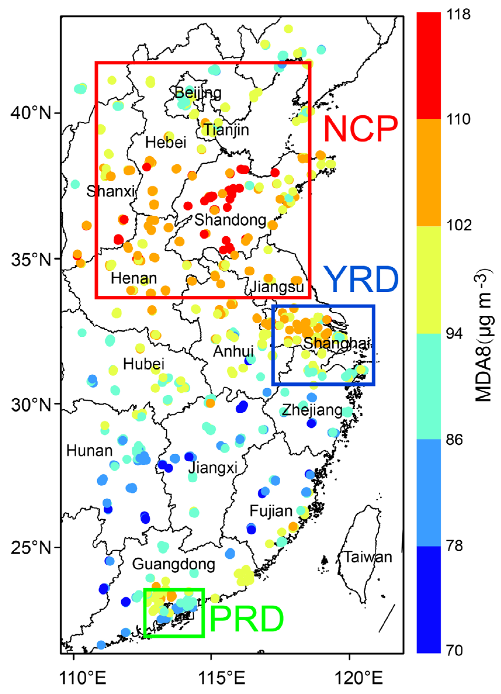
The hourly surface ozone concentration observations from 778 ground-based sites from the National Surface Air Quality Observation Network of China were utilized to construct a surface ozone estimation model in East China. The in situ surface ozone measurements from 1 January 2019 to 31 December 2021 were acquired from the China National Environmental Monitoring Center. To assure basic data quality, the 8 h moving average ozone concentration was calculated only when there were at least six valid measurements in those 8 h time periods. Subsequently, the maximum 8 h averaged surface ozone value during each day was extracted as the MDA8 value. At the same time, another quality control measure was applied to filter out records with inadequate samples. To avoid the possibility of reducing the accuracy of surface ozone estimation due to the different number of samples in each data record, the hourly ozone records with surface ozone data missing for ten consecutive days in a month were excluded, and records with more than 30% of samples missing during the study period were also rejected. To reduce the mutual interference between sites that were too close to each other and better establish the ozone estimation model, the observations of 778 sites in East China were clustered into 447 sites using a distance threshold of 0.05°. The spatial distribution of 447 ozone observation sites in East China is shown in Figure 1, below.
2.2. Ozone Precursors
As ozone is mainly generated by the photochemical oxidation of volatile organic compounds (VOCs) and carbon monoxide (CO) and in the presence of nitrogen oxides (NOX) and sunlight, it is of great significance to include these two primary ozone precursors, including VOCs and NOX, in the subsequent surface ozone estimation model. Since the spatial coverage and spatial resolution of the daily available CO product (MOPITT data) are not able to fulfill the need of the surface ozone estimation, the satellite CO data were not included in this work. In this study, satellite-based daily NO2 and HCHO data from Sentinel-5P-TROPOMI (S5P) products (7 km × 3.5 km), the NO2 mass mixing ratio at 1000 hPa, and HCHO total column density reanalysis datasets from the Copernicus Atmosphere Monitoring Service (CAMS) products (0.1° × 0.1°), as well as CAMS emission inventory NOX products between 2019 and 2021, were used to establish the surface ozone estimation model of East China. In addition, six kinds of VOC inventory datasets (including C3H8, C5H8, CH4, H2O2, OH, and PAN) derived from the CAMS emission inventory between 2019 and 2021 (0.1° × 0.1°) were also utilized to establish the surface ozone estimation model. Furthermore, the spatial resolution of these ozone precursor datasets was resampled to the same 0.05° × 0.05° grid for spatial matching. To be in line with MDA8, the daily averages of six kinds of VOCs, CAMS-HCHO, and CAMS-NO2 concentration datasets were calculated. In addition, since the CAMS-NOX data are monthly emission inventory data, the same CAMS-NOx data were used for each day of a particular month.
2.3. Meteorological Factors
The spatial–temporal variations in surface ozone are largely regulated by anthropogenic emissions (i.e., ozone precursors) and meteorological conditions [10,43]. Simultaneously, as other kinds of factors modulating surface ozone variations, meteorological factors were considered comprehensively here to establish the surface ozone estimation model. These meteorological factors, including surface 2 m temperature (T), relative humidity (RH), surface pressure (SP), boundary layer height (BLH), wind speed (WS), wind direction (WD), total cloud cover (TCC), and total precipitation (TP), as well as UV radiation (UV) derived from ERA5 reanalysis datasets between 2019 and 2021 with 0.1° × 0.1° spatial resolution, were used in this work. To acquire better surface ozone estimation accuracy and be consistent with previous studies [43], daily accumulated values of UV radiation and TP, daily averages of RH, SP, BLH, and TCC, daily maximum T, and hourly values of WS and WD at 14:00 pm (at which the highest MDA8 and temperature is oftentimes observed) were extracted and utilized in the surface ozone estimation model. All meteorological factor datasets were resampled to the same 0.05° × 0.05° grid for modeling and surface ozone estimation. Detailed descriptions and performances of these widely used datasets have been well documented in previous studies [44,45,46,47].
2.4. Auxiliary Data
In addition to ozone precursors and meteorological factors, elevation data (DEM), satellite-based Normalized Difference Vegetation Index (NDVI) data, the Land Use and Land Cover data (LULC), population density data (POPU), and CAMS O3 reanalysis products (CAMS-O3) were also used to establish the surface ozone estimation model of East China. In this study, the DEM data with 30 m spatial resolution were derived from the China Resource and Environmental Science Data Center (CRESDC). Similarly, the POPU data of 1 km × 1 km spatial resolution for China from 2019 to 2021 were also obtained from CRESDC, and the annual population values of each city were corrected with its statistical yearbook before being used for surface ozone estimation. The LULC data were divided into nine ground class attributes (including LULC1~LULC9) between 2019 and 2021 with 30 m × 30 m spatial resolution. In addition, the NDVI data used in this study were the 16-day MOD13C1 product derived from the Moderate-resolution Imaging Spectroradiometer (MODIS) onboard the Terra satellite. The NDVI data between 2019 and 2021 with 0.05° × 0.05° spatial resolution were used in this study to establish the surface ozone estimation model. To better estimate surface ozone over East China, CAMS reanalysis products of O3 mass mixing ratio at 1000 hPa (0.1° × 0.1°) were used in this study as an influencing factor on surface ozone because these data contain surface ozone information. Similar to CAMS-HCHO, the daily averaged CAMS-O3 concentration was calculated to match the daily MDA8.
All the explanatory variables collected, including ozone precursors datasets, meteorological data, DEM data, POPU data, LULC data, and CAMS-O3 data, were resampled to 0.05° × 0.05° grids for the subsequent surface ozone estimation. On the time scale, since population and LULC are annual datasets, the same population and LULC data were used for each day within a given year to match the daily MDA8. Similarly, the same NDVI data were used for each day within a given 16-day period. After sites with limited samples were excluded, daily MDA8 time series were paired with daily time series of collocated explanatory variables including ozone precursors, meteorological factors, DEM data, NDVI data, LULC data, and POPU data at 447 monitoring sites according to the location and date. All the datasets used in this study are summarized in Table S1.
3. Methods
3.1. Statistical Modeling Methods
Machine learning methods, an extension of the traditional statistical model, have been widely used in air pollutant estimation in recent years due to their excellent performances [48,49,50]. Furthermore, among these machine learning models, the eXtreme Gradient Boosting (XGBoost) model, a popular statistical modeling method, was utilized to establish the surface ozone estimation model for East China. The XGBoost model was utilized in this work due to its fast training speed, high prediction accuracy, and ability to quantify the relative importance of input variables [27,36,51,52]. Subsequently, four XGBoost surface ozone estimation models in East China using different NO2 and HCHO datasets were established by combining NO2 and HCHO data from satellite monitoring (S5P-TROPOMI) and reanalysis data (CAMS), as follows:
where O3-surface denotes the ground-based MDA8 observations; NO2-S5P and HCHO-S5P denote the tropospheric column density of NO2 and HCHO data in the corresponding site and date; and T, UV, RH, SP, BLH, WS, WD, TCC, and TP are the surface 2 m temperature, UV radiation, relative humidity at 1000 hPa, surface pressure, boundary layer height, wind speed, wind direction, total cloud cover, and total precipitation, respectively. Six kinds of CAMS VOCs inventory datasets (including C3H8, C5H8, CH4, H2O2, OH, and PAN) were also utilized as a separate influencing factor of surface ozone in the surface ozone estimation model. For simplicity, these six kinds of VOCs are uniformly summarized as VOCs in Equation (1). DEM and NDVI denote the elevation and Normalized Difference Vegetation Index of the corresponding site and date. Similarly, POPU and LULC represent the population density and classification of land use types, respectively.
O3-surface ~ f (NO2-S5P/NO2-CAMS + HCHO-S5P/HCHO-CAMS + O3-CAMS + VOCs + NOX-CAMS + T
+ UV + RH + SP + BLH + WS + WD + TCC + TP + DEM + NDVI + POPU + LULC)
+ UV + RH + SP + BLH + WS + WD + TCC + TP + DEM + NDVI + POPU + LULC)
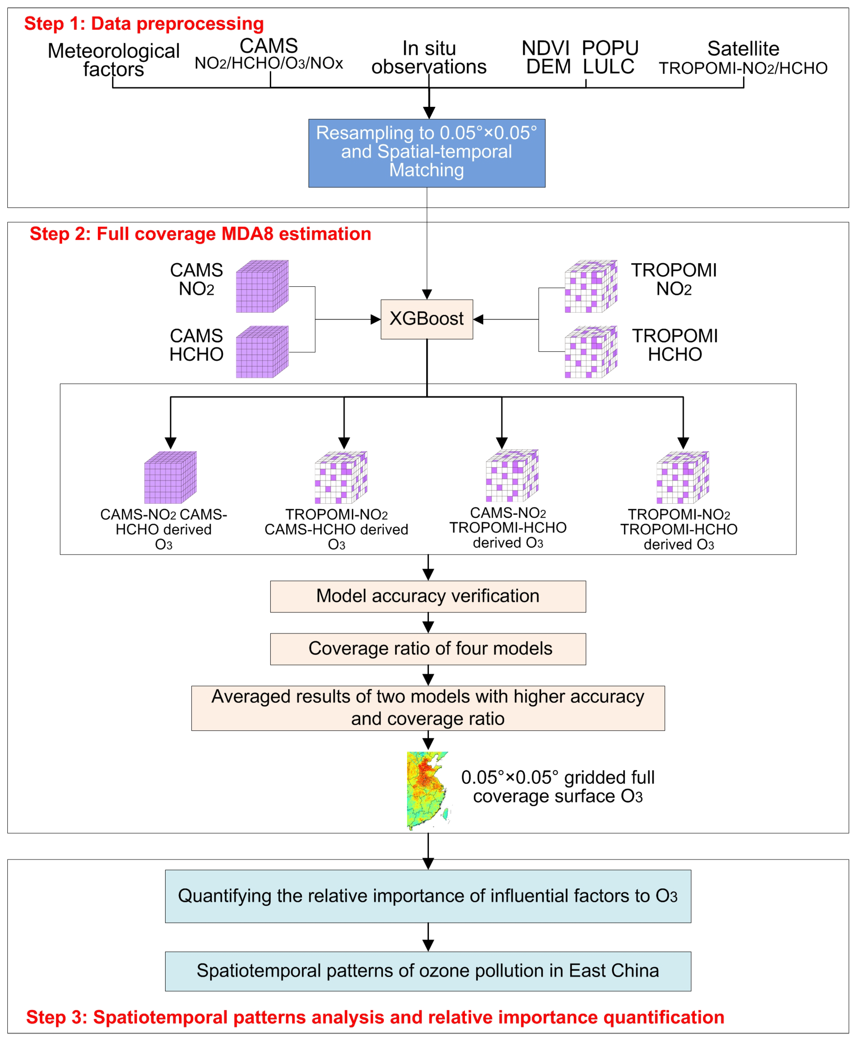
As the training target datasets of the surface ozone estimation model, the MDA8 observations of 778 sites in East China were clustered into 447 sites using the distance threshold of 0.05°. Subsequently, in the model training process, 5% of the 447 sites were randomly chosen as sites-based validation datasets, and then 80% of the input data samples in the remaining 95% of sites were random selected as the training samples, while 20% of the input data samples were randomly chosen as sample-based validation datasets. In terms of the XGBoost model, the booster type was gbtree, and the number of boost rounds was 500. Subsequently, the relative importance of each influencing factor was quantified in the surface ozone estimation XGBoost models because the XGBoost model has the capability to quantify the relative importance of input variables. Finally, to improve the robustness of the MDA8 estimation model, the model estimation results of 50 training trials were saved and averaged, and the averaged result was used as the final gridded MDA8 concentration estimation. The data processing flow and methodology of this study is shown in Figure 2.
3.2. Accuracy Evaluation Statistics
After the surface ozone estimation models were established by the XGBoost model, the prediction accuracy of these four combinations of NO2 and HCHO datasets from satellite monitoring (S5P-TROPOMI) and reanalysis data (CAMS) were evaluated and compared. In this work, four commonly used statistical indicators, including the R2, root-mean-squared error (RMSE), mean prediction error (MPE), and relative percentage error (RPE), were calculated between the spatiotemporal co-located observed MDA8 and model-estimated MDA8 to quantitatively assess the accuracy and model performance. These four statistical indicators can be described as the following equations:
where denotes observed in situ MDA8, and represents the estimated MDA8, respectively. is the arithmetic means of the observed MDA8 values, and n denotes the number of data pairs.
After the prediction accuracy of these four combinations was evaluated and compared, the combination of NO2 and HCHO with the higher prediction accuracy and higher spatiotemporal coverage ratio of MDA8 estimation results was chosen as the final surface ozone estimation combination. Subsequently, the final chosen surface ozone estimation models were utilized to estimate the daily 0.05° × 0.05° gridded MDA8 data over East China during 2019–2021. In addition, the spatial–temporal distribution of MDA8 over East China, the spatial and temporal patterns of the ozone pollution in East China (MDA8 > 160 µg m−3), were revealed, and the impact of the COVID-19 epidemic on ozone pollution in East China was compared and analyzed.
4. Results
4.1. The Model Verification Performance
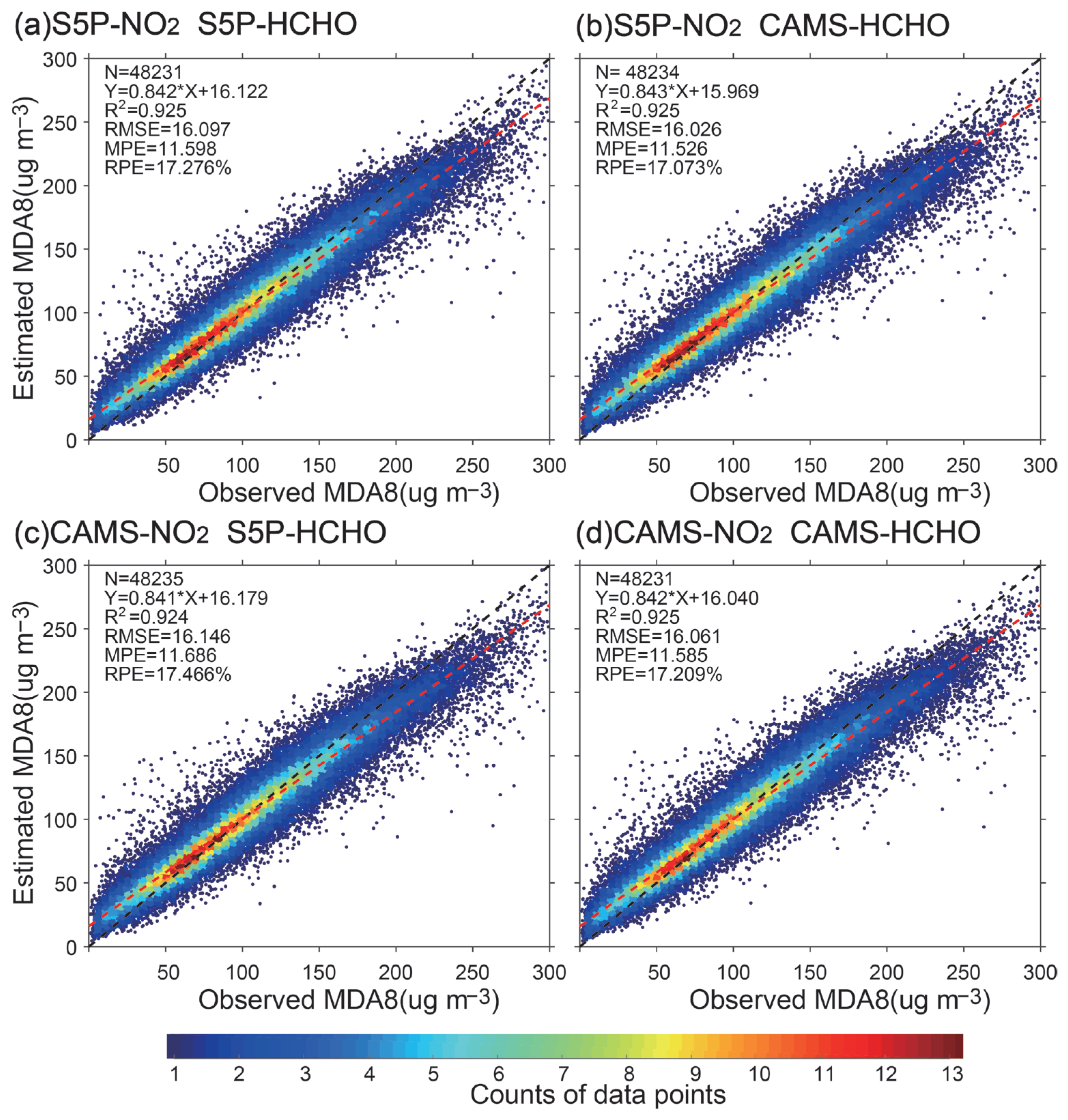
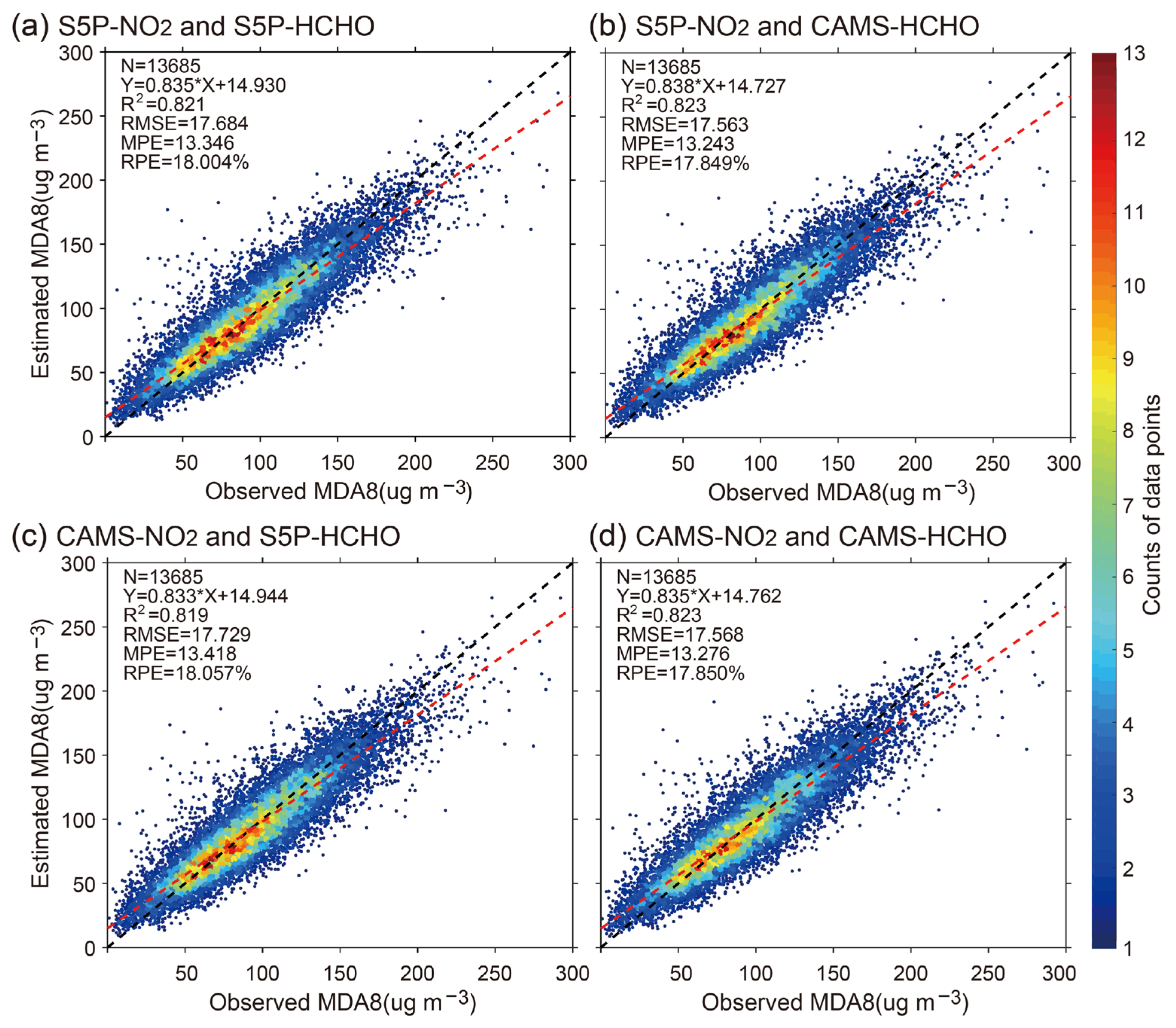
Figure 3 and Figure 4 show the sample-based and site-based validation results of four ozone estimation XGBoost models using four kinds of data combinations, including S5P-TROPOMI NO2 and S5P-TROPOMI HCHO, S5P-TROPOMI NO2 and CAMS HCHO, CAMS NO2 and S5P-TROPOMI HCHO, and CAMS NO2 and CAMS HCHO. In the model training process, 5% of 447 sites (22 sites) were randomly chosen, and all data pairs from these sites were then considered as the site validation dataset. Subsequently, 80% of the data pairs from the remaining 95% of 447 sites (425 sites) were randomly selected as training samples, while the remaining 20% of the input data pairs were selected as the sample-based validation dataset. This indicated that the forecasted MDA8 concentrations exhibited a high correlation with ground-based MDA8 measurements in all four models. The sample-based validation results shown in Figure 3 indicate that all four O3 estimation models had high prediction accuracies, the R2 values of these four models were all larger than 0.923, the RMSE values were all smaller than 16.15 µg m−3, the MPE values were smaller than 11.69 µg m−3, and the RPE values were smaller than 17.47%. In terms of the site-based validation prediction accuracy of these four MDA8 estimation models (Figure 4), the R2 values of four models were all larger than 0.82, the RMSE values were all smaller than 17.73 µg m−3, the MPE values were smaller than 13.42 µg m−3, and the RPE values were smaller than 18.10%. Among these four MDA8 estimation models, the ozone estimation model using S5P-TROPOMI NO2 and CAMS HCHO and the ozone estimation model using CAMS NO2 and CAMS HCHO had higher prediction accuracy, with their R2 values both larger than 0.823, RMSE values both smaller than 17.57 µg m−3, the MPE values both smaller than 13.28 µg m−3, and RPE values both smaller than 17.85%. Among these four MDA8 estimation models, the ozone estimation model using S5P-TROPOMI NO2 and CAMS HCHO and the ozone estimation model using CAMS NO2 and CAMS HCHO had higher prediction accuracy, with the RMSE values both smaller than 16.07 µg m−3, the MPE values both smaller than 11.59 µg m−3, and RPE values both smaller than 17.21%.
In addition to the site-based and sample-based validation results of the four models, the spatiotemporal coverage ratios of the four MDA8 estimation results are also revealed in Figure S1. The results indicated that the spatiotemporal coverage of the two surface ozone estimation models with the S5P-TROPOMI HCHO as the input variable was lower in the four models. The estimation results of the model using S5P-TROPOMI NO2 and S5P-TROPOMI HCHO had the lowest spatiotemporal coverage ratio, with a value of 68.46%, while the estimation results of the model using CAMS NO2 and S5P-TROPOMI HCHO had the second-lowest coverage ratio, with a value of 70.31%. In contrast, the estimation results of the model using CAMS NO2 and CAMS HCHO had the highest spatiotemporal coverage ratio, with a value of 100%, while the estimation results of the model using S5P-TROPOMI NO2 and CAMS HCHO had the second-highest coverage ratio, with a value of 96.26%.
In general, the results of four MDA8 estimation models revealed that the model using S5P-TROPOMI NO2 and CAMS HCHO and the other model using CAMS NO2 and CAMS HCHO showed better prediction accuracy and higher coverage for estimation results, with higher R2 values, lower RMSE values, lower MPE values, lower RPE values, and a higher coverage ratio. Subsequently, these two MDA8 estimation models were chosen to produce the final MDA8 estimation results. To improve the robustness of the MDA8 estimation model, 50 training trial results of each chosen MDA8 estimation model were saved. Subsequently, the 100 independent model estimation results of these two models were averaged and considered as the final gridded MDA8 concentration estimation results. The final MDA8 estimation dataset is a daily 0.05° × 0.05° gridded product of East China during 2019–2021.
4.2. Relative Importance of Each Explanatory Variable
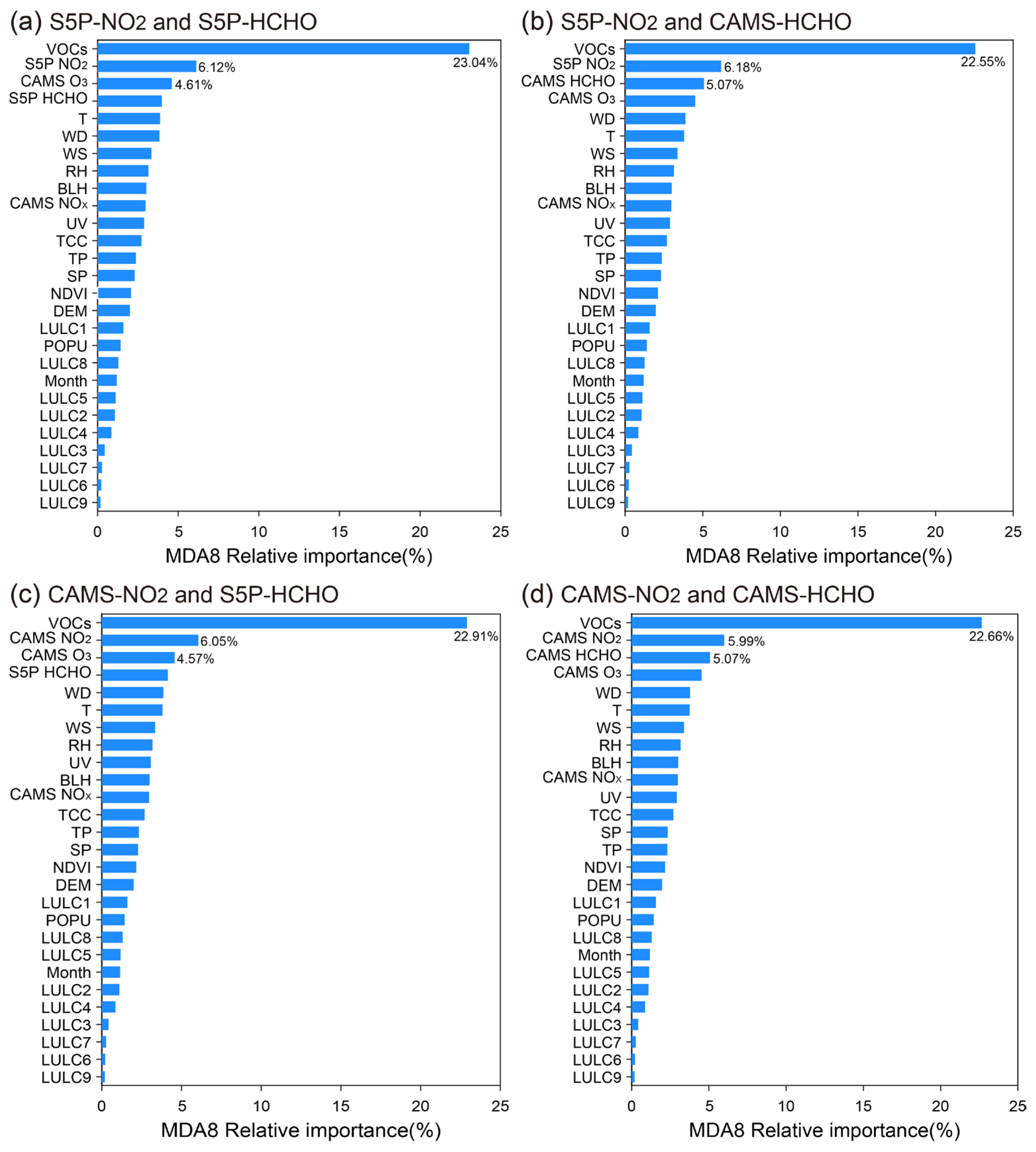
The relative importance of explanatory variables for surface ozone is depicted in Figure 5. In these four surface ozone estimation models, VOCs were found to be the dominant factor, with the relative importance values larger than 22.55% for the MDA8 concentration in East China. This result indicates that the ambient ozone concentration is obviously modulated by VOCs. Combining the results of the four O3 estimation models, it revealed that the two largest contributors to these six VOCs (including C3H8, C5H8, CH4, H2O2, OH, and PAN) were C3H8 and H2O2, which contributed about 4.12% and 4.06%, respectively, and the remaining four VOCs including C5H8, OH, PAN, and CH4, contributed 4.02%, 3.79%, 3.55%, and 3.49%, respectively. Subsequently, the relative importance of NO2 (S5P NO2 or CAMS NO2) was larger than 6% in these four models, and the relative importance of CAMS NOX was about 2.97% in these four models, and it was revealed that the NOX (including NO2) was the second principal variable for the surface ozone in East China. CAMS-NOX is emission inventory data of anthropogenic emissions, while S5P-NO2 is satellite-based observations, and the combination of these two types of data contains NOX information from different sources, which can better estimate the surface O3. In addition to VOCs and NOX, HCHO (including S5P HCHO and CAMS HCHO) was found to be the third or fourth primary factor for the surface ozone with a relative importance larger than 4%, and this reemphasized the important contribution of VOCs to surface ozone. CAMS O3 was revealed to be the third or fourth dominant factor for the surface ozone in East China, with a relative importance larger than 4.51%.
In terms of meteorological factors, the sum contribution of T, WS, WD, RH, BLH, UV, TCC, TP, and SP constituted 27.35% of the overall variable importance. Among these meteorological factors, T, WS, and WD were considered to be the three most important meteorological factors for the O3 pollution, all with a relative importance larger than 3.4%. High temperature, weak wind speed, and stable atmospheric conditions, and a downwind region of polluted air mass was favored by the photochemical generation of ambient O3, as was revealed by previous studies [34,43,53]. In addition, RH, BLH, and UV were also treated as three major drivers for the O3 pollution over East China. This could be attributed to the appropriated relative humidity and stronger UV radiation that are the proper conditions of the photochemical generation of ambient O3, and the BLH would affect the vertical exchange of the polluted air mass [54,55]. In addition, TCC, TP, and SP also played significant roles in the O3 pollution, which was consistent with many previous studies [34,56,57].
In addition to these ozone precursors and meteorological factors, NDVI played an important role in ozone pollution; this may be attributed to more plants emitting more biogenic isoprene, thereby promoting the elevation of O3 concentration [27,58]. Subsequently, DEM, LULC, POPU, and Month also played important roles in surface ozone pollution. This may be attributed to time potentially influencing the temperature and UV radiation, a greater population leading to more pollution emissions and, in turn, to increased ozone pollution, and a higher elevation potentially affecting the distribution of population and sunshine, thereby promoting the elevation of O3 concentration [27,58].
In general, VOCs and NOX were revealed to be the top two main influencing factors of O3 pollution in East China. The implementation of VOCs and NOX emission reductions in East China will help to significantly reduce O3 pollution levels and control O3 pollution in this region. This provides a reference for the control of O3 pollution and ensures the sustainable development of the environment in East China. At the same time, the control of O3 pollution supports the protection of human health and the sustainability of citizens’ lives in East China. Moreover, the control of O3 pollution helps to protect ecosystems and crop yield, and also provides a guarantee for the sustainability of food security in East China.
4.3. Spatial Distribution of Estimated MDA8 over East China
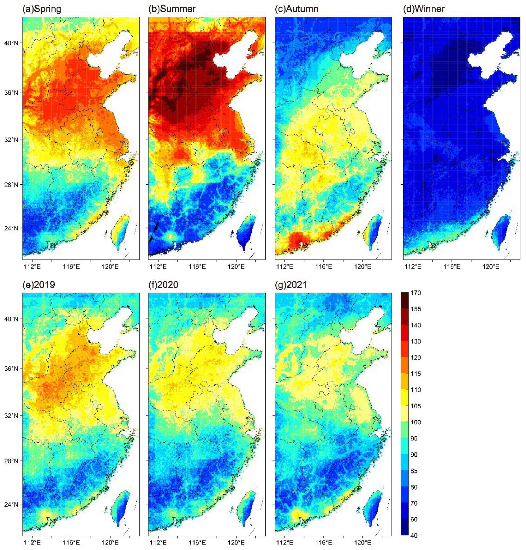
Figure 6 depicts the spatial patterns of the seasonal and annual average MDA8 estimated by the XGBoost model from 1 January 2019 to 31 December 2021. The results of the estimated MDA8 indicated evident high surface ozone pollution levels in several specific regions. The first region that attracts attention had the most serious ozone pollution in the NCP. This major ozone pollution region included Beijing–Tianjin–Hebei, Shandong Province, Henan Province, and the northern part of the Anhui and Jiangsu provinces. At the same time, the region closest to the level of ozone pollution in the NCP was the YRD and the PRD. However, the scope of the ozone pollution in the YRD and the PRD was not as large as that of the NCP.
In terms of the spatial patterns of the seasonal MDA8, the most serious ozone pollution (>115 µg m−3) was found in North China in summer. This major ozone pollution region included Beijing–Tianjin–Hebei, Shandong Province, Henan Province, Shanxi Province, the southern part of Liaoning Province, the eastern part of Hubei Province, and the northern part of the Anhui and Jiangsu provinces. Although the spatial coverage of ozone pollution in spring is similar to that in summer, the ozone pollution level in North China in spring is lower than that in summer. The most serious ozone pollution in autumn is mainly concentrated in the PRD and the coastal area of the border area between Guangdong Province and Fujian Province; although its regional scope is much smaller than that of the NCP, its ozone pollution level is similar to that of the NCP in summer. Among the four seasons, the season with the most serious ozone pollution is summer, and the lightest ozone pollution level occurs in winter. The spatial distribution of seasonally averaged MDA8 in East China is consistent with the results of previous studies, which may be related to the spatial distribution of ozone precursor emissions (VOCs and NOX), temperature, and UV radiation [21,22,38,47].
From the perspective of the temporal variation in MDA8 in East China during 2019–2021, although the largest ozone pollution concentration region and the highest ozone pollution level occurred in the NCP, the ozone pollution level in this region decreased from 2019 to 2021, and the spatial coverage of ozone pollution also decreased year by year. In 2019, the major ozone pollution regions included Beijing–Tianjin–Hebei, Shandong Province, Henan Province, and the northern part of Anhui Province and Jiangsu Province. However, in 2021, the main areas of ozone pollution were narrowed to only include southern Hebei Province, western Shandong Province, northern Henan Province, and northern Anhui Province and Jiangsu Province. In addition, the ozone pollution level in the Ji–Lu–Yu region (including Hebei Province, Henan Province, and Shandong Province) decreased from 115 µg m−3 in 2019 to 105 µg m−3 in 2020, and this may have contributed to the impact of the synergistic control measures of PM2.5 and O3 implemented by the Chinese government and the impact of the COVID-19 pandemic (February–May 2020). At the same time, the reduction in O3 precursors and the nationwide lockdown measures led to the reduction in emissions from human activities and reduced the net photochemical production of ozone, which in turn reduced ozone pollution levels in the NCP in 2020. The decreasing trend of ozone pollution in 2019–2021 is consistent with the previous study, which may be related to the synergistic control measures of PM2.5 and O3 implemented by the Chinese government, as well as to the continued influence of COVID-19 in China [38,59,60].
4.4. Spatiotemporal Distribution of Estimated MDA8 Exceedance over China
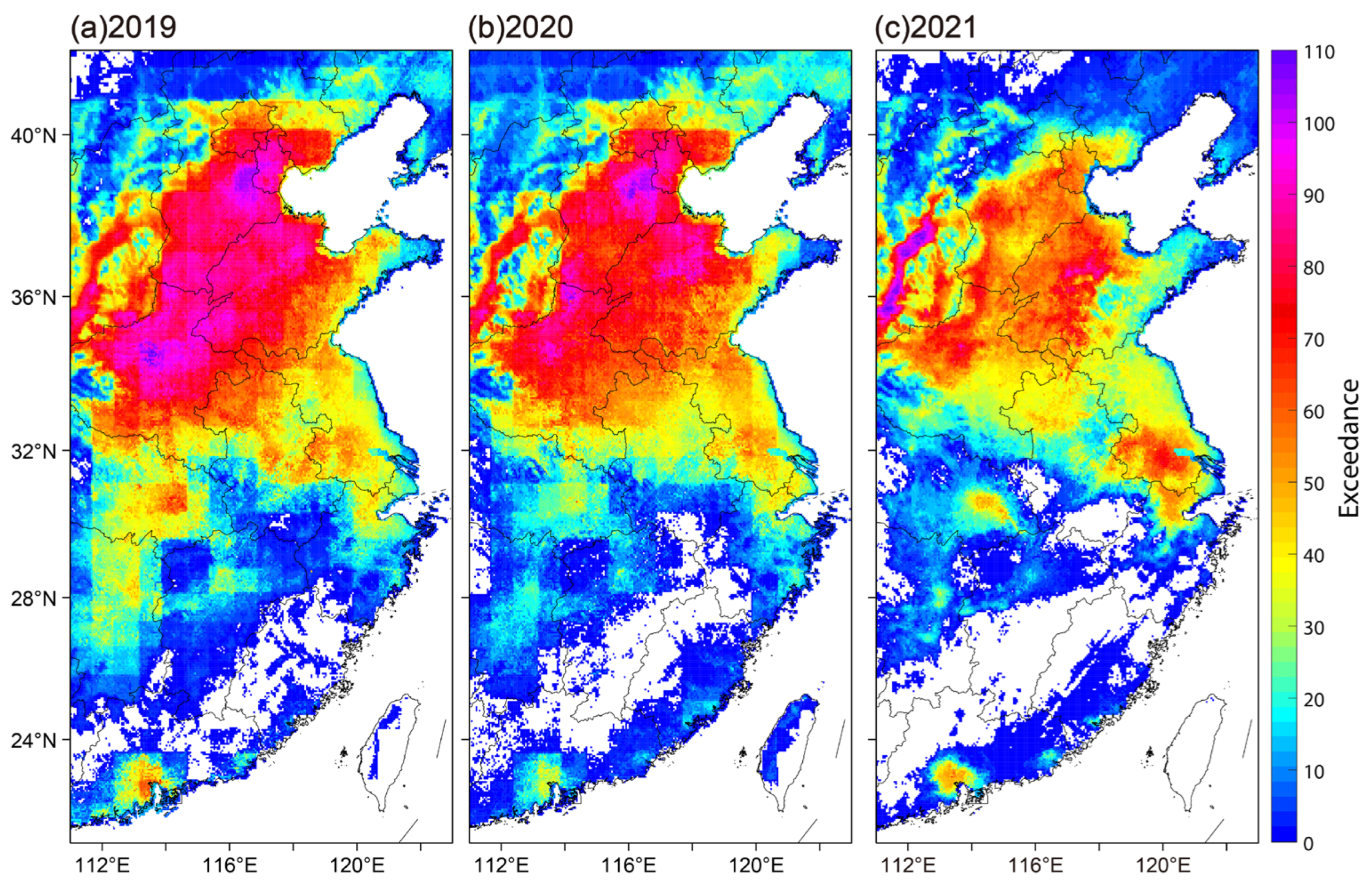
Figure 7 depicts the annual accumulated exceedance (MDA8 > 160 µg m−3) of estimated MDA8 for each pixel of East China during 2019–2021. The results derived from the spatial distribution of accumulated exceedance on each pixel indicated that ozone pollution in the NCP was worst over East China. The severity of the ozone pollution in the NCP was the highest, and the coverage of the ozone pollution in the NCP was also the largest in China. From the perspective of the interannual variation of ozone pollution, ozone pollution in the NCP decreased during 2019–2020. During these two years, the reduction in ozone pollution in the NCP between 2019 and 2020 attracted the most attention. Compared with 2019, the severity and spatial coverage of ozone pollution in 2020 in the NCP reduced significantly in both aspects, and this phenomenon might be ascribed to the impact of COVID-19. As an area closer to Hubei Province, the initial center of the epidemic, the closure of the city during the COVID-19 epidemic caused a reduction in the intensity of human activities in the NCP in the first half of 2020, and the reduced intensity of human activities led to the reduction in ozone pollution precursor emissions, thereby reducing the level of ozone pollution in the NCP. Similar to the NCP, the ozone pollution level in southeastern Hubei Province, the PRD, and the YRD also decreased between 2019 and 2020, and this might also be ascribed to the impact of COVID-19.
Compared with 2020, the severity and spatial coverage of ozone pollution in 2021 in the NCP were greatly reduced in both aspects. However, ozone pollution in southeastern Hubei Province, the PRD, and the YRD showed different annual variation characteristics, and the results revealed that ozone pollution in these regions increased from 2020 to 2021. In addition, this result revealed that the regional terrain and the climatic conditions in these regions were different from those in the NCP, and the ozone pollution variation characteristic was also different from that in the NCP. The decrease in O3 pollution levels from 2019 to 2021 may be due to the impact of the policy on the synergistic management of PM2.5 and O3 pollution implemented by the government [38,61]. Additionally, the COVID-19 epidemic reappeared in 2021 in China, and this may also have led to the decrease in ozone pollution level, resulting in a further decrease in O3 pollution in the NCP in 2021 [38,61,62].
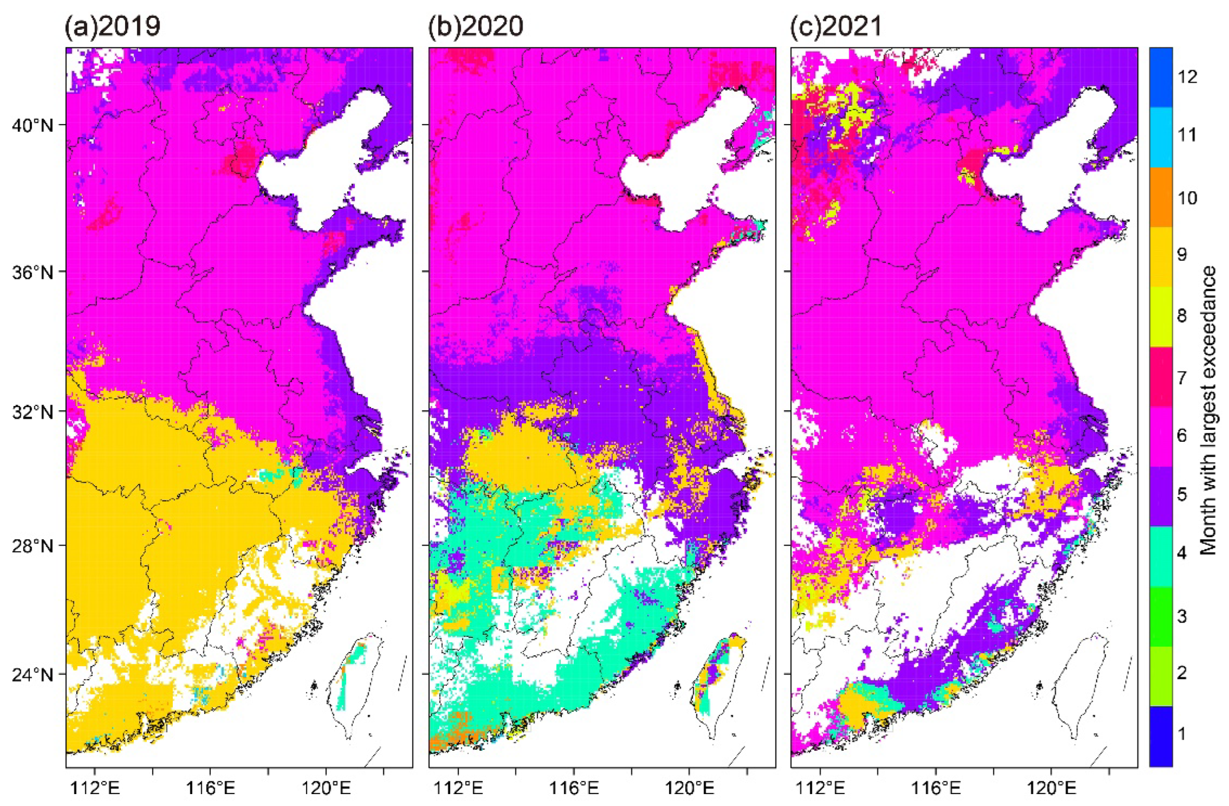
Figure 8 depicts the spatial distribution of the month with the largest exceedance in each pixel during 2019–2021. The results revealed that the time characteristic of ozone pollution varied greatly in different regions of East China. In most parts of the NCP, the month with the highest frequency of ozone pollution occurred in June from 2019 to 2021, while in 2020 alone, the worst month for ozone pollution was May in the southern part of Henan Province, Anhui Province, and the southern part of Jiangsu Province. Similar to the NCP, the most serious ozone pollution in Shanxi Province was measured in June from 2019 to 2021, and only in the northern part of Shanxi Province did the most serious ozone pollution occur in July and May of 2020.
In contrast to the NCP, ozone pollution during 2019–2021 in the YRD mainly occurred in May. In terms of ozone pollution in the Middle and Lower of Yangtze Plain (MLYP) and South China, the worst ozone pollution in 2019 and 2020 mainly occurred in September and April, respectively, while in 2021 the most serious ozone pollution happened in May and June in most parts of these two regions. Similar to the YRD, the ozone pollution in 2019–2021 in Liaoning Province and the eastern part of Shandong Province mainly occurred in May. In general, ozone pollution in the NCP usually happens in summer, while ozone pollution in the YRD, Central China, Northeastern China, and South China mainly occurs in autumn and spring. The spatial distribution of seasonal O3 pollution in East China is consistent with the results of previous studies, and this could be related to the differences in the spatiotemporal patterns of the temperature and UV radiation in East China [22,34,38,47,59].
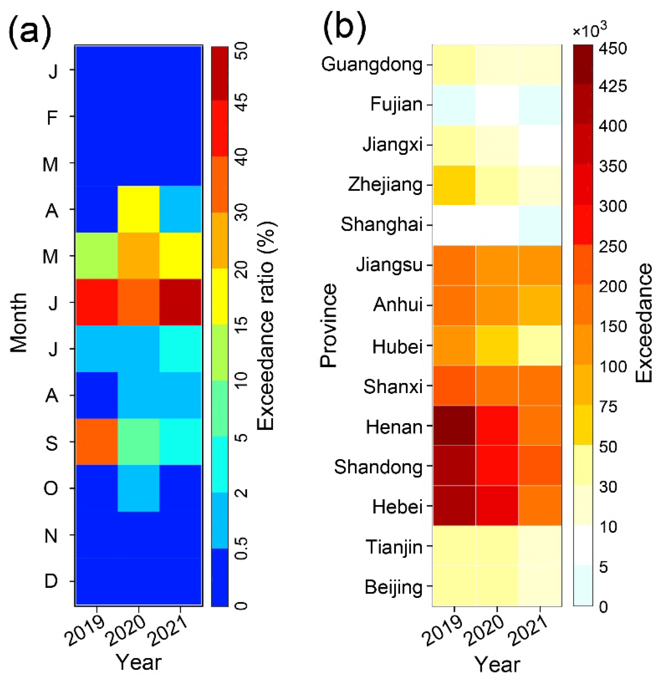
To reveal the annual variation in ozone pollution for each month and each province during 2019–2021, Figure 9 depicts the exceedance (MDA8 > 160 μg m−3) ratio of ozone pollution in each month and the accumulated exceedance in each province of East China for each year. In the process of calculating the exceedance ratio of ozone pollution in each month, the cumulative value of the number of days with ozone pollution (MDA8 > 160 μg m−3) for all pixels in East China for a given month of a year was first calculated. Subsequently, the number of pixels in East China was multiplied by the number of days in that month of that year. Finally, the ratio of the two values produced the final ozone exceedance ratio for that month of that year. The results in Figure 9a indicate that the ozone pollution in China varied greatly in different years and different months. From the perspective of the monthly variation in ozone pollution, it is indicated that June was the month with the highest level of ozone pollution, and the averaged exceedance ratio for June was 42.65% in the period 2019–2021. Compared to June 2020, the higher exceedance ratio of ozone pollution in June 2021 may be due to enhanced net ozone photochemical production resulting from higher temperatures in June 2021 [63]. Following June, May was the month with the second most serious ozone pollution, with an averaged exceedance ratio value of 16.90% in the period 2019–2021. Additionally, September was the month with the third most significant ozone pollution, and the mean exceedance ratio was 15.56% over 3 years. In addition to the above three months, the most severe ozone pollution happened in April and July. In general, the ozone pollution in China mainly occurred in summer, followed by spring, and then in autumn. Summer was the season with the most ozone pollution incidents in China between 2019 and 2021.
To compare the degree of ozone pollution in different provinces and reveal the interannual variation in ozone pollution in each province of East China, Figure 9b reveals the annual accumulative exceedance of ozone pollution in each province of East China in the period 2019–2021. The top three provinces with serious ozone pollution were Hebei, Shandong, and Henan, and the cumulative annual exceedance of MDA8 in each of these three provinces was more than 163,000. Following these three provinces, the annual MDA8 exceedance values of Shanxi, Anhui, and Jiangsu were all near or larger than 86,000. In addition, ozone pollution in Hubei was also serious, with an annual MDA8 exceedance larger than 40,000. In terms of the spatial distribution of aggregation characteristics for the annual exceedance of these 14 provinces, the ozone pollution was mainly concentrated in the NCP. Consistent with the results of previous studies, emissions of ozone precursors (including VOCs and NOX) in the NCP are the highest in China, and consequently, the O3 pollution level in the NCP is higher than in other regions of China [22,47,64]. From the perspective of the interannual changes in various provinces, ozone pollution in most of the top 7 provinces with serious ozone pollution eased in the period 2019–2021, and it was consistent with the results shown in Figure 6 and Figure 7. In addition, the seven provinces with the least serious ozone pollution were Fujian, Shanghai, Jiangxi, Guangdong, Tianjin, and Beijing. Furthermore, the regions with better air quality (i.e., less ozone pollution) were mainly distributed in most parts of South China, the YRD, and parts of North China. Finally, compared with the annual exceedance of MDA8 in 2019, the value in 2020 was smaller in most provinces, and this indicated that the ozone pollution was eased by COVID-19 in early 2020 due to the reduction in the intensity of human activity.
4.5. Possible Impact of COVID-19 on the Estimated MDA8 in East China
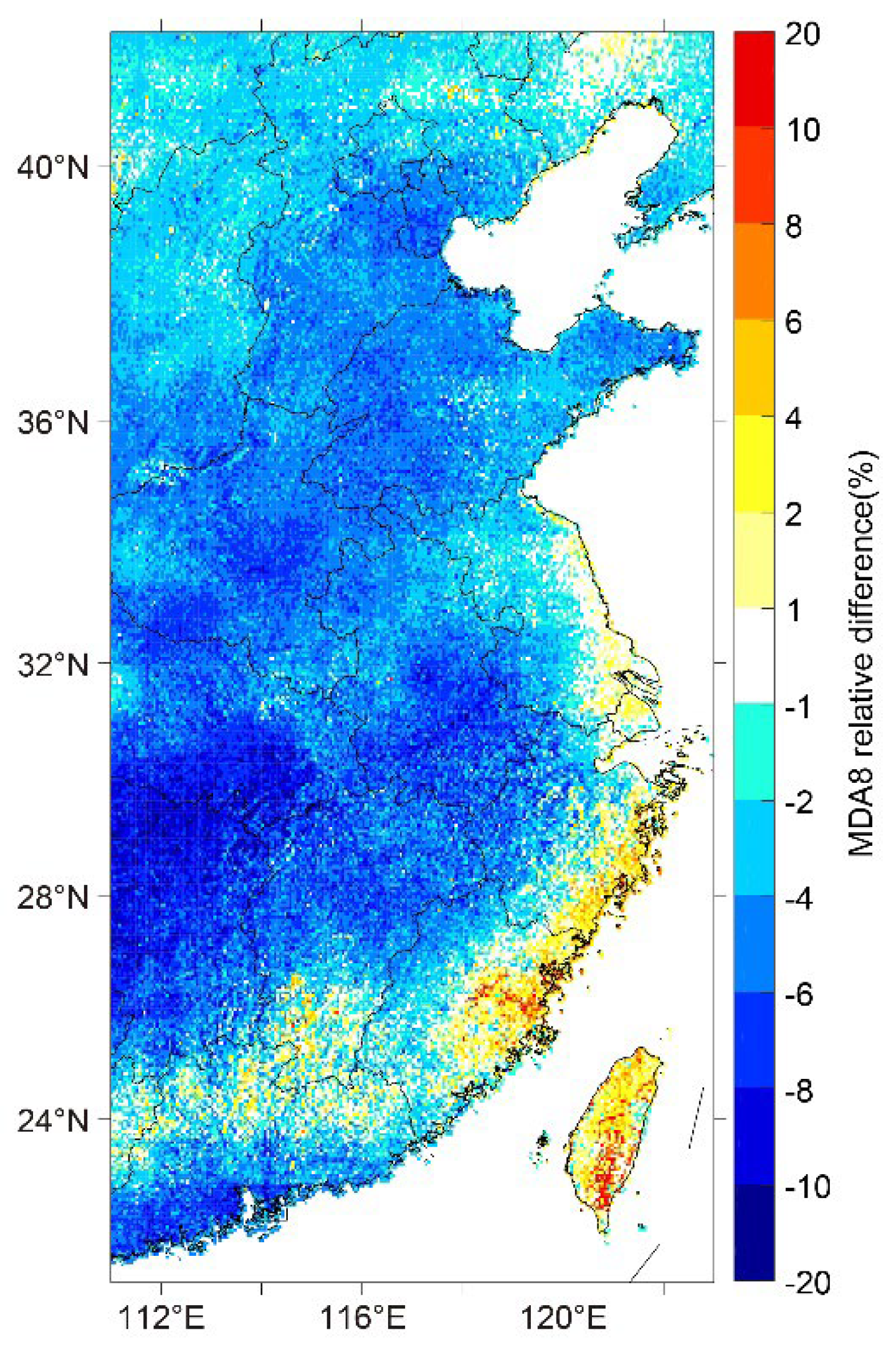
To further understand the possible impact of COVID-19 on surface ozone concentration in China during the lockdown, the spatial variability of the relative difference in MDA8 in East China between 2020 (during the COVID-19 epidemic) and 2019 (one year before the COVID-19 epidemic) is revealed in Figure 10. Wuhan was the first city in China to be isolated due to COVID-19, and its lockdown period began on 23 January 2020. Following Wuhan, other cities went into lockdown by 29 January 2020, until 2 May 2020, when the national lockdown was lifted. The surface ozone concentration in most parts of East China decreased in 2020 compared to 2019. In contrast, there were fewer regions with increased ozone concentration during 2019–2020, mainly concentrated in the eastern coastal areas of Jiangsu, Shanghai, Zhejiang, and Fujian.
In terms of the magnitude of the ozone concentration reduction in East China, the ozone concentration in the Middle and Lower of Yangtze Plain (MLYP) had the largest reduction, of 6–10%, and the spatial scope of ozone concentration declining in the region was also the widest. In addition to the MLYP, the PRD was the other region with the largest reduction in ozone concentration, with a 4–10% reduction in 2020 compared to 2019. Following the MLYP and the PRD, the NCP is another region with a large reduction in ozone concentration, with ozone pollution levels in 2020 decreasing by 2–8% compared to 2019, and it is also the region with the widest spatial coverage of ozone pollution reduction in East China. This is probably due to the NCP, the MLYP, and the PRD being close to Wuhan, the center of the COVID-19 epidemic, and in these regions, the degree of resumption of work and production was low and far from the fully recovered level before the epidemic. Previous studies have shown that during the COVID-19 epidemic, HCHO (VOCs) and NOx emissions decreased in North China, which may have led to the reduction in ozone content in the NCP and its surrounding areas [65,66].
On the other hand, the ozone concentration in 2020 in eastern coastal areas of Jiangsu, Shanghai, Zhejiang, and Fujian increased by 1–8% compared to 2019 during the lockdown period. These regions are dominated by export-oriented economies. Additionally, the personal activities of residents decreased in 2020, but the activities of epidemic-prevention-related industries did not stop, they picked up and led to higher emissions. This is likely to be the reason why the ozone pollution in this area has increased compared to 2019, although it was affected by the COVID-19 epidemic between January and May 2020. In 2020, due to the COVID-19 epidemic, the foreign exports of the Yangtze River Delta increased and Ningbo Port experienced cargo ship congestion, which indirectly confirms the presence of foreign trade and production in the southeast coastal region [67].
In general, due to the impact of the COVID-19 epidemic and the implementation of the policy on the synergistic management of PM2.5 and O3 pollution in China, the average surface O3 concentration in East China from January to June 2020 decreased by 3.74% compared with the same period in 2019. The regions most affected by the COVID-19 epidemic were the NCP, the MLYP, and the PRD, and the ozone pollution level in these areas has been significantly reduced. The regions least affected by the COVID-19 epidemic were the eastern coastal areas of Jiangsu, Shanghai, Zhejiang, and Fujian, and the ozone pollution in these areas has been significantly increased by 1–8%.
5. Discussion
Most previous studies on large-scale surface ozone estimation utilized the deterministic model, and their validation R2 values were lower, with a range from 0.40 to 0.67 [6,16,21]. Additionally, the spatial resolution of the model estimation results was generally coarser than 0.1° × 0.1° [6,16,21]. In terms of the statistical model, the machine learning model was used to estimate the MDA8 of China; however, most of these studies focused on the ozone prediction of a single city or an urban belt [13,26,28,29,30,31,32,33,34,35], and the spatial distribution of these results is limited. For large-scale surface ozone estimation studies using the statistical model, the accuracy of the ozone estimation results is high [27,37,38]. However, the spatial resolution of surface ozone estimation results in most studies is 0.1° × 0.1° or coarser [39,40], and only a few studies estimated 0.05° × 0.05° surface ozone products [41,42]. Additionally, NO2 and HCHO observations with a high spatial resolution derived from S5P-TROPOMI (7 km × 3.5 km) are rarely used by existing surface ozone estimation studies [41,42]; therefore, it is necessary to use the high-spatial-resolution precursors’ data (S5P-TROPOMI NO2 and HCHO) to estimate large-scale surface ozone and obtain the surface ozone estimation results with higher accuracy, higher certainty, and higher spatial resolution.
In this study, daily HCHO and NO2 observations derived from S5P-TROPOMI (7 km × 3.5 km) were used to build the surface ozone estimation model. Subsequently, the XGBoost model was utilized to establish a surface ozone estimation model in East China during 2019–2021. The sample-based validation results indicated that the prediction accuracy of these four surface ozone estimation models is high, with the R2 values all larger than 0.92, while the site-based validation prediction R2 values of these models were all larger than 0.82. The prediction accuracy of surface ozone estimations in this study (sample-based R2: 0.92) is close to that of the coarser resolution (0.1° × 0.1°) results in previous studies. Subsequently, the daily 0.05° × 0.05° gridded MDA8 data over East China during 2019–2021 was estimated. In the future, long time-series nationwide daily 0.05° × 0.05° gridded MDA8 data estimation should be carried out based on deep learning methods to obtain surface ozone products with a longer time series, larger scale range, and higher accuracy.
6. Conclusions
In this study, NO2 and HCHO derived from S5P-TROPOMI (7 km × 3.5 km), meteorological data, CAMS NO2 and HCHO data, CAMS VOCs data, CAMS NOX emission inventory, MODIS NDVI data, DEM data, population density data, land use and land cover data, and in situ surface ozone observations from the national air quality monitoring networks in China between 2019 and 2020 were utilized to develop a large-scale surface ozone estimation model for East China. Subsequently, four XGBoost surface ozone estimation models in East China using different NO2 and HCHO datasets were established by combining NO2 and HCHO data from satellite monitoring (S5P-TROPOMI) and reanalysis data (CAMS). The site-based validation prediction accuracy of these four MDA8 estimation models was high, the R2 values of four models were all larger than 0.82, the RMSE values were all smaller than 17.73 µg m−3, the MPE values were smaller than 13.42 µg m−3, and the RPE values were smaller than 18.10%. In terms of the spatiotemporal coverage ratios of the four MDA8 estimation results, it revealed that the coverage ratio of the estimation results from the model using CAMS NO2 and CAMS HCHO was the highest (100%), while the coverage ratio of the estimation results from the model using S5P-TROPOMI NO2 and CAMS HCHO was the second highest, with a value of 96.26%.
Furthermore, the MDA8 estimation results of these two models were chosen and averaged as the final surface ozone estimation product, and daily 0.05° × 0.05° gridded MDA8 data over East China during 2019–2021 were estimated. This indicated that O3 pollution in East China during 2019–2021 was susceptible to anthropogenic precursors such as VOCs (22.55%) and NOX (8.97%), as well as meteorological factors (27.35%) such as wind direction, temperature, and wind speed. Subsequently, the spatial patterns of the MDA8 were revealed, and the spatiotemporal patterns of the ozone exceedance in East China in different years and different months were described and analyzed. It was revealed that ozone pollution in East China exhibits complex spatial and temporal variation characteristics. Ozone pollution in East China is mainly concentrated in the NCP, the PRD, and the YRD. Among these three regions, ozone pollution in the NCP mainly occurs in June (summer), ozone pollution in the YRD mainly occurs in May (late spring), and ozone pollution in the PRD mainly occurs in April (spring) and September (autumn). In addition, nationwide ozone pollution in 2020 was reduced by 3.74% due to the impact of the COVID-19 epidemic. The regions affected the most by the COVID-19 epidemic were the NCP (−2~−8%), the Middle and Lower of Yangtze Plain (−6~−10%), and the PRD (−4~−10%). Overall, the results showed that VOCs were the most important influencing factor on surface ozone, and NOx was the second most important contributing factor in East China, which reflected the urgency and importance of VOCs and NOx emission reductions in East China. Thus, the implementation of VOCs and NOX emission reductions in East China will help to significantly reduce O3 pollution levels and control O3 pollution in this region. This provides a reference for the control of O3 pollution and ensures the sustainable development of the environment in East China. At the same time, the control of O3 pollution supports the protection of human health and the sustainability of citizens’ lives in East China. Moreover, the control of O3 pollution helps to protect the ecosystems and crop yields and also provides a guarantee for the sustainability of food security in the region.
Supplementary Materials
The following supporting information can be downloaded at: https://www.mdpi.com/article/10.3390/su16010123/s1. Table S1. A brief summary of datasets used in this study. Figure S1. Spatiotemporal coverage ratio of four surface ozone estimation models.
Author Contributions
Conceptualization, M.M. and F.M.; methodology, M.M., M.L. (Mengjiao Liu) and M.L. (Mengnan Liu); validation, M.M., M.L. (Mengjiao Liu), M.L. (Mengnan Liu), F.M. and Y.W.; formal analysis, M.M., F.M., H.X., Y.W. and M.L. (Mengjiao Liu); data curation, M.M.; writing—original draft preparation, M.M.; writing—review and editing, F.M.; visualization, M.M., M.L. (Mengjiao Liu) and M.L. (Mengnan Liu); supervision, M.M. and F.M.; project administration, M.M. and F.M.; funding acquisition, M.M. and H.X. All authors have read and agreed to the published version of the manuscript.
Funding
This work was supported by the National Natural Science Foundation of China (Grant No. 42301382), the Shandong Provincial Natural Science Foundation (Grant No. ZR2021QD034, Grant No. ZR2022YQ36), the Youth Innovation Team Project of Higher School in Shandong Province (Grant No. 2022KJ201), and the opening Research Funds of the Henan Polytechnic University’s Key Laboratory of Mine Spatial Information Technologies of National Administration of Surveying, Mapping and Geoinformation (KLM2018).
Institutional Review Board Statement
Not applicable.
Informed Consent Statement
Not applicable.
Data Availability Statement
The data utilized in this study were obtained from the China National Environmental Monitoring Center (CNEMC), the TROPOMI group, the MODIS group, and the China Resource and Environmental Science Data Center (CRESDC) for providing DEM and population density data, ECMWF, and the Copernicus Atmosphere Monitoring Service (CAMS). Data are available from the authors upon request, and with permission from CNEMC, the TROPOMI group, the MODIS group, the CRESDC, ECMWF, and CAMS.
Acknowledgments
The authors are grateful to the China National Environmental Monitoring Center (CNEMC) for making observations of surface ozone (“http://www.cnemc.cn (accessed on 15 December 2023)”), the TROPOMI group for providing HCHO data and NO2 data (“https://dataspace.copernicus.eu/ (accessed on 15 December 2023)”), the MODIS group for providing NDVI data (“https://ladsweb.modaps.eosdis.nasa.gov/search/ (accessed on 15 December 2023)”), the China Resource and Environmental Science Data Center for providing DEM and population density data (“https://www.resdc.cn/Default.aspx (accessed on 15 December 2023)”), ECMWF for providing ERA5 reanalysis (“https://cds.climate.copernicus.eu/#!/search?text=ERA5 (accessed on 15 December 2023)”), and the Copernicus Atmosphere Monitoring Service (CAMS, “ https://ads.atmosphere.copernicus.eu/cdsapp#!/search?text=CAMS (accessed on 15 December 2023)”) for providing emissions reanalysis data.
Conflicts of Interest
The authors declare no conflict of interest.
References
- Al-Salihi, A.M.; Hassan, Z.M. Temporal and Spatial Variability and Trend Investigation of Total Ozone Column over Iraq Employing Remote Sensing Data: 1979–2012. Int. Lett. Chem. Phys. Astron. 2015, 53, 1–18. [Google Scholar] [CrossRef]
- De Laat, A.T.J.; Van Der A, R.J.; Van Weele, M. Tracing the second stage of ozone recovery in the Antarctic ozone-hole with a “big data” approach to multivariate regressions. Atmos. Chem. Phys. 2015, 15, 79–97. [Google Scholar] [CrossRef]
- Lipsett, M.J.; Ostro, B.D.; Reynolds, P.; Goldberg, D.; Hertz, A.; Jerrett, M.; Smith, D.F.; Garcia, C.; Chang, E.T.; Bernstein, L. Long-term exposure to air pollution and cardiorespiratory disease in the California teachers study cohort. Am. J. Respir. Crit. Care Med. 2011, 184, 828–835. [Google Scholar] [CrossRef]
- Karlsson, P.E.; Klingberg, J.; Engardt, M.; Andersson, C.; Langner, J.; Karlsson, G.P.; Pleijel, H. Past, present and future concentrations of ground-level ozone and potential impacts on ecosystems and human health in northern Europe. Sci. Total Environ. 2017, 576, 22–35. [Google Scholar] [CrossRef]
- Stowell, J.D.; Kim, Y.-m.; Gao, Y.; Fu, J.S.; Chang, H.H.; Liu, Y. The impact of climate change and emissions control on future ozone levels: Implications for human health. Environ. Int. 2017, 108, 41–50. [Google Scholar] [CrossRef] [PubMed]
- Liu, H.; Liu, S.; Xue, B.; Lv, Z.; Meng, Z.; Yang, X.; Xue, T.; Yu, Q.; He, K. Ground-level ozone pollution and its health impacts in China. Atmos. Environ. 2018, 173, 223–230. [Google Scholar] [CrossRef]
- Fowler, D.; Pilegaard, K.; Sutton, M.A.; Ambus, P.; Raivonen, M.; Duyzer, J.; Simpson, D.; Fagerli, H.; Fuzzi, S.; Schjoerring, J.K.; et al. Atmospheric composition change: Ecosystems-Atmosphere interactions. Atmos. Environ. 2009, 43, 5193–5267. [Google Scholar] [CrossRef]
- Moura, B.B.; Hoshika, Y.; Ribeiro, R.V.; Paoletti, E. Exposure- and flux-based assessment of ozone risk to sugarcane plants. Atmos. Environ. 2018, 176, 252–260. [Google Scholar] [CrossRef]
- Harmens, H.; Hayes, F.; Mills, G.; Sharps, K.; Osborne, S.; Pleijel, H. Wheat yield responses to stomatal uptake of ozone: Peak vs rising background ozone conditions. Atmos. Environ. 2018, 173, 1–5. [Google Scholar] [CrossRef]
- Li, P.; De Marco, A.; Feng, Z.; Anav, A.; Zhou, D.; Paoletti, E. Nationwide ground-level ozone measurements in China suggest serious risks to forests. Environ. Pollut. 2018, 237, 803–813. [Google Scholar] [CrossRef]
- Zhang, Y.; Cooper, O.R.; Gaudel, A.; Thompson, A.M.; Nédélec, P.; Ogino, S.Y.; West, J.J. Tropospheric ozone change from 1980 to 2010 dominated by equatorward redistribution of emissions. Nat. Geosci. 2016, 9, 875–879. [Google Scholar] [CrossRef] [PubMed]
- Xie, B.; Zhang, H.; Yang, D.D.; Wang, Z.L. A modeling study of effective radiative forcing and climate response due to increased methane concentration. Adv. Clim. Chang. Res. 2016, 7, 241–246. [Google Scholar] [CrossRef]
- Lv, B.; Cobourn, W.G.; Bai, Y. Development of nonlinear empirical models to forecast daily PM2.5 and ozone levels in three large Chinese cities. Atmos. Environ. 2016, 147, 209–223. [Google Scholar] [CrossRef]
- Wang, T.; Xue, L.; Brimblecombe, P.; Lam, Y.F.; Li, L.; Zhang, L. Ozone pollution in China: A review of concentrations, meteorological influences, chemical precursors, and effects. Sci. Total Environ. 2017, 575, 1582–1596. [Google Scholar] [CrossRef] [PubMed]
- Lu, X.; Hong, J.; Zhang, L.; Cooper, O.R.; Schultz, M.G.; Xu, X.; Wang, T.; Gao, M.; Zhao, Y.; Zhang, Y. Severe Surface Ozone Pollution in China: A Global Perspective. Environ. Sci. Technol. Lett. 2018, 5, 487–494. [Google Scholar] [CrossRef]
- Lu, X.; Zhang, L.; Chen, Y.; Zhou, M.; Zheng, B.; Li, K.; Liu, Y.; Lin, J.; Fu, T.M.; Zhang, Q. Exploring 2016–2017 surface ozone pollution over China: Source contributions and meteorological influences. Atmos. Chem. Phys. 2019, 19, 8339–8361. [Google Scholar] [CrossRef]
- Sun, L.; Xue, L.; Wang, Y.; Li, L.; Lin, J.; Ni, R.; Yan, Y.; Chen, L.; Li, J.; Zhang, Q.; et al. Impacts of meteorology and emissions on summertime surface ozone increases over central eastern China between 2003 and 2015. Atmos. Chem. Phys. 2019, 19, 1455–1469. [Google Scholar] [CrossRef]
- Li, K.; Jacob, D.J.; Liao, H.; Shen, L.; Zhang, Q.; Bates, K.H. Anthropogenic drivers of 2013–2017 trends in summer surface ozone in China. Proc. Natl. Acad. Sci. USA 2019, 116, 422–427. [Google Scholar] [CrossRef]
- Li, K.; Jacob, D.; Shen, L.; Lu, X.; De Smedt, I.; Liao, H. 2013–2019 increases of surface ozone pollution in China: Anthropogenic and meteorological influences. Atmos. Chem. Phys. Discuss. 2020, 20, 11423–11433. [Google Scholar] [CrossRef]
- Gong, C.; Liao, H.; Zhang, L.; Yue, X.; Dang, R.; Yang, Y. Persistent ozone pollution episodes in North China exacerbated by regional transport. Environ. Pollut. 2020, 265, 115056. [Google Scholar] [CrossRef]
- Liu, Y.; Wang, T. Worsening urban ozone pollution in China from 2013 to 2017—Part 2: The effects of emission changes and implications for multi-pollutant control. Atmos. Chem. Phys. 2020, 20, 6323–6337. [Google Scholar] [CrossRef]
- Ma, M.; Yao, G.; Guo, J.; Bai, K. Distinct spatiotemporal variation patterns of surface ozone in China due to diverse influential factors. J. Environ. Manag. 2021, 288, 112368. [Google Scholar] [CrossRef] [PubMed]
- Hoshyaripour, G.; Brasseur, G.; Andrade, M.F.; Gavidia-Calderón, M.; Bouarar, I.; Ynoue, R.Y. Prediction of ground-level ozone concentration in São Paulo, Brazil: Deterministic versus statistic models. Atmos. Environ. 2016, 145, 365–375. [Google Scholar] [CrossRef]
- Zhang, Y.; Bocquet, M.; Mallet, V.; Seigneur, C.; Baklanov, A. Real-time air quality forecasting, part I: History, techniques, and current status. Atmos. Environ. 2012, 60, 632–655. [Google Scholar] [CrossRef]
- Ryu, Y.H.; Hodzic, A.; Barre, J.; Descombes, G.; Minnis, P. Quantifying errors in surface ozone predictions associated with clouds over the CONUS: A WRF-Chem modeling study using satellite cloud retrievals. Atmos. Chem. Phys. 2018, 18, 7509–7525. [Google Scholar] [CrossRef]
- Gao, M.; Yin, L.; Ning, J. Artificial neural network model for ozone concentration estimation and Monte Carlo analysis. Atmos. Environ. 2018, 184, 129–139. [Google Scholar] [CrossRef]
- Li, R.; Zhao, Y.; Zhou, W.; Meng, Y.; Zhang, Z.; Fu, H. Developing a novel hybrid model for the estimation of surface 8 h ozone (O3) across the remote Tibetan Plateau during 2005–2018. Atmos. Chem. Phys. 2020, 20, 6159–6175. [Google Scholar] [CrossRef]
- Cai, M.; Yin, Y.; Xie, M. Prediction of hourly air pollutant concentrations near urban arterials using artificial neural network approach. Transp. Res. Part D Transp. Environ. 2009, 14, 32–41. [Google Scholar] [CrossRef]
- Tie, X.; Geng, F.; Peng, L.; Gao, W.; Zhao, C. Measurement and modeling of O3 variability in Shanghai, China: Application of the WRF-Chem model. Atmos. Environ. 2009, 43, 4289–4302. [Google Scholar] [CrossRef]
- Feng, Y.; Zhang, W.; Sun, D.; Zhang, L. Ozone concentration forecast method based on genetic algorithm optimized back propagation neural networks and support vector machine data classification. Atmos. Environ. 2011, 45, 1979–1985. [Google Scholar] [CrossRef]
- Lin, K.M.; Yu, T.Y.; Chang, L.F. Establishment of a structural equation model for ground-level ozone: A case study at an urban roadside site. Environ. Monit. Assess. 2014, 186, 8317–8328. [Google Scholar] [CrossRef] [PubMed]
- Xue, L.K.; Wang, T.; Gao, J.; Ding, A.J.; Zhou, X.H.; Blake, D.R.; Wang, X.F.; Saunders, S.M.; Fan, S.J.; Zuo, H.C.; et al. Ground-level ozone in four Chinese cities: Precursors, regional transport and heterogeneous processes. Atmos. Chem. Phys. 2014, 14, 13175–13188. [Google Scholar] [CrossRef]
- Lu, W.Z.; Wang, D. Learning machines: Rationale and application in ground-level ozone prediction. Appl. Soft Comput. J. 2014, 24, 135–141. [Google Scholar] [CrossRef]
- Zhao, W.; Fan, S.; Guo, H.; Gao, B.; Sun, J.; Chen, L. Assessing the impact of local meteorological variables on surface ozone in Hong Kong during 2000–2015 using quantile and multiple line regression models. Atmos. Environ. 2016, 144, 182–193. [Google Scholar] [CrossRef]
- Mok, K.M.; Yuen, K.V.; Hoi, K.I.; Chao, K.M.; Lopes, D. Predicting ground-level ozone concentrations by adaptive Bayesian model averaging of statistical seasonal models. Stoch. Environ. Res. Risk Assess. 2018, 32, 1283–1297. [Google Scholar] [CrossRef]
- Zhan, Y.; Luo, Y.; Deng, X.; Grieneisen, M.L.; Zhang, M.; Di, B. Spatiotemporal prediction of daily ambient ozone levels across China using random forest for human exposure assessment. Environ. Pollut. 2018, 233, 464–473. [Google Scholar] [CrossRef]
- Li, T.; Wu, J.; Chen, J.; Shen, H. An Enhanced Geographically and Temporally Weighted Neural Network for Remote Sensing Estimation of Surface Ozone. IEEE Trans. Geosci. Remote Sens. 2022, 60, 1–13. [Google Scholar] [CrossRef]
- Wei, J.; Li, Z.; Li, K.; Dickerson, R.R.; Pinker, R.T.; Wang, J.; Liu, X.; Sun, L.; Xue, W.; Cribb, M. Full-coverage mapping and spatiotemporal variations of ground-level ozone (O3) pollution from 2013 to 2020 across China. Remote Sens. Environ. 2022, 270, 112775. [Google Scholar] [CrossRef]
- Dai, H.; Huang, G.; Wang, J.; Zeng, H. VAR-Tree Model Based Spatio-Temporal Characterization and Prediction of O3 Concentration in China. Ecotox. Environ. Safe. 2023, 257, 114960. [Google Scholar] [CrossRef]
- Mu, X.; Wang, S.; Jiang, P.; Wang, B.; Wu, Y.; Zhu, L. Full-Coverage Spatiotemporal Estimation of Surface Ozone over China Based on a High-Efficiency Deep Learning Model. Int. J. Appl. Earth Obs. Geoinf. 2023, 118, 103284. [Google Scholar] [CrossRef]
- Li, T.; Yang, Q.; Wang, Y.; Wu, J. Joint Estimation of PM2.5 and O3 over China Using a Knowledge-Informed Neural Network. Geosci. Front. 2023, 14, 101499. [Google Scholar] [CrossRef]
- Zeng, Q.; Wang, Y.; Tao, J.; Fan, M.; Zhu, S.; Chen, L.; Wang, L.; Li, Y. Estimation of Ground-Level O3 Concentration in the Yangtze River Delta Region Based on a High-Performance Spatiotemporal Model MixNet. Sci. Total Environ. 2023, 896, 165061. [Google Scholar] [CrossRef] [PubMed]
- Fix, M.J.; Cooley, D.; Hodzic, A.; Gilleland, E.; Russell, B.T.; Porter, W.C.; Gabriele, G.P. Observed and predicted sensitivities of extreme surface ozone to meteorological drivers in three US cities. Atmos. Environ. 2018, 176, 292–300. [Google Scholar] [CrossRef]
- Dee, D.P.; Uppala, S.M.; Simmons, A.J.; Berrisford, P.; Poli, P.; Kobayashi, S.; Andrae, U.; Balmaseda, M.A.; Balsamo, G.; Bauer, P.; et al. The ERA-Interim reanalysis: Configuration and performance of the data assimilation system. Q. J. R. Meteorol. Soc. 2011, 137, 553–597. [Google Scholar] [CrossRef]
- Bai, K.; Chang, N.; Gao, W. Quantification of relative contribution of Antarctic ozone depletion to increased austral extratropical precipitation during 1979–2013. J. Geophys. Res. 2016, 121, 1459–1474. [Google Scholar] [CrossRef]
- Guo, J.; Miao, Y.; Zhang, Y.; Liu, H.; Li, Z.; Zhang, W.; He, J.; Lou, M.; Yan, Y.; Bian, L.; et al. The climatology of planetary boundary layer height in China derived from radiosonde and reanalysis data. Atmos. Chem. Phys. 2016, 16, 13309–13319. [Google Scholar] [CrossRef]
- Ma, M.; Bai, K.; Qiao, F.; Shi, R.; Gao, W. Quantifying impacts of crop residue burning in the North China Plain on summertime tropospheric ozone over East Asia. Atmos. Environ. 2018, 194, 14–30. [Google Scholar] [CrossRef]
- Bai, K.; Li, K.; Sun, Y.; Wu, L.; Zhang, Y.; Chang, N.-B.; Li, Z. Global synthesis of two decades of research on improving PM2.5 estimation models from remote sensing and data science perspectives. Earth-Sci. Rev. 2023, 241, 104461. [Google Scholar] [CrossRef]
- Bai, K.; Li, K.; Guo, J.; Cheng, W.; Xu, X. Do More Frequent Temperature Inversions Aggravate Haze Pollution in China? Geophys. Res. Lett. 2022, 49, e2021GL096458. [Google Scholar] [CrossRef]
- Bai, K.; Li, K.; Ma, M.; Li, K.; Li, Z.; Guo, J.; Chang, N.-B.; Tan, Z.; Han, D. LGHAP: The Long-Term Gap-free High-resolution Air Pollutant concentration dataset, derived via tensor-flow-based multimodal data fusion. Earth Syst. Sci. Data 2022, 14, 907–927. [Google Scholar] [CrossRef]
- Wu, C.; Li, K.; Bai, K. Validation and Calibration of CAMS PM2.5 Forecasts Using In situ PM2.5 Measurements in China and United States. Remote Sens. 2020, 5, 3813. [Google Scholar] [CrossRef]
- Li, R.; Cui, L.; Hongbo, F.; Li, J.; Zhao, Y.; Chen, J. Satellite-based estimation of full-coverage ozone (O3) concentration and health effect assessment across Hainan Island. J. Clean. Prod. 2020, 244, 118773. [Google Scholar] [CrossRef]
- Tawfik, A.B.; Steiner, A.L. A proposed physical mechanism for ozone-meteorology correlations using land-atmosphere coupling regimes. Atmos. Environ. 2013, 72, 50–59. [Google Scholar] [CrossRef]
- Li, K.; Chen, L.; Ying, F.; White, S.J.; Jang, C.; Wu, X.; Gao, X.; Hong, S.; Shen, J.; Azzi, M.; et al. Meteorological and chemical impacts on ozone formation: A case study in Hangzhou, China. Atmos. Res. 2017, 196, 40–52. [Google Scholar] [CrossRef]
- Kaser, L.; Patton, E.G.; Pfister, G.G.; Weinheimer, A.J.; Montzka, D.D.; Flocke, F.; Thompson, A.M.; Stauffer, R.M.; Halliday, H.S. The effect of entrainment through atmospheric boundary layer growth on observed and modeled surface ozone in the Colorado front range. J. Geophys. Res. 2017, 122, 6075–6093. [Google Scholar] [CrossRef]
- Yi, K.; Liu, J.; Ban-Weiss, G.; Zhang, J.; Tao, W.; Cheng, Y.; Tao, S. Response of the global surface ozone distribution to Northern Hemisphere sea surface temperature changes: Implications for long-range transport. Atmos. Chem. Phys. 2017, 17, 8771–8788. [Google Scholar] [CrossRef]
- Yadav, R.; Sahu, L.K.; Beig, G.; Jaaffrey, S.N.A. Role of long-range transport and local meteorology in seasonal variation of surface ozone and its precursors at an urban site in India. Atmos. Res. 2016, 176–177, 96–107. [Google Scholar] [CrossRef]
- Hewitt, C.N.; Ashworth, K.; Boynard, A.; Guenther, A.; Langford, B.; MacKenzie, A.R.; Misztal, P.K.; Nemitz, E.; Owen, S.M.; Possell, M.; et al. Ground-level ozone influenced by circadian control of isoprene emissions. Nat. Geosci. 2011, 4, 671–674. [Google Scholar] [CrossRef]
- Ma, M.; Liu, M.; Liu, M.; Li, K.; Xing, H.; Meng, F. Resolving contributions of NO2 and SO2 to PM2.5 and O3 pollutions in the North China Plain via multi-task learning. J. Appl. Remote Sens. 2023, 18, 012004. [Google Scholar] [CrossRef]
- Xiang, S.; Liu, J.; Tao, W.; Yi, K.; Xu, J.; Hu, X.; Liu, H.; Wang, Y.; Zhang, Y.; Yang, H.; et al. Control of both PM2.5 and O3 in Beijing-Tianjin-Hebei and the surrounding areas. Atmos. Environ. 2020, 224, 117259. [Google Scholar] [CrossRef]
- Li, K.; Jacob, D.J.; Liao, H.; Zhu, J.; Shah, V.; Shen, L.; Bates, K.H.; Zhang, Q.; Zhai, S. A two-pollutant strategy for improving ozone and particulate air quality in China. Nat. Geosci. 2019, 12, 906–910. [Google Scholar] [CrossRef]
- Liu, Y.; Wang, T.; Stavrakou, T.; Elguindi, N.; Doumbia, T.; Granier, C.; Bouarar, I.; Gaubert, B.; Brasseur, G.P. Diverse response of surface ozone to COVID-19 lockdown in China. Sci. Total Environ. 2021, 789, 147739. [Google Scholar] [CrossRef] [PubMed]
- Gao, M.; Wang, F.; Ding, Y.; Wu, Z.; Xu, Y.; Lu, X.; Wang, Z.; Carmichael, G.R.; McElroy, M. Large-scale climate patterns offer preseasonal hints on the co- occurrence of heat wave and O3 pollution in China. Proc. Natl. Acad. Sci. USA 2023, 120, e2218274120. [Google Scholar] [CrossRef] [PubMed]
- Liang, X.; Chen, X.; Zhang, J.; Shi, T.; Sun, X.; Fan, L.; Wang, L.; Ye, D. Reactivity-based industrial volatile organic compounds emission inventory and its implications for ozone control strategies in China. Atmos. Environ. 2017, 162, 115–126. [Google Scholar] [CrossRef]
- Li, K.; Jacob, D.J.; Liao, H.; Qiu, Y.; Shen, L.; Zhai, S.; Bates, K.H.; Sulprizio, M.P.; Song, S.; Lu, X.; et al. Ozone pollution in the North China Plain spreading into the late-winter haze season. Proc. Natl. Acad. Sci. USA 2021, 118, e2015797118. [Google Scholar] [CrossRef] [PubMed]
- Zhang, Q.; Pan, Y.; He, Y.; Walters, W.W.; Ni, Q.; Liu, X.; Xu, G.; Shao, J.; Jiang, C. Substantial nitrogen oxides emission reduction from China due to COVID-19 and its impact on surface ozone and aerosol pollution. Sci. Total Environ. 2021, 753, 142238. [Google Scholar] [CrossRef] [PubMed]
- Hou, W.; Shi, Q.; Guo, L. Impacts of COVID-19 pandemic on foreign trade intermodal transport accessibility: Evidence from the Yangtze River Delta region of mainland China. Transp. Res. Part A Policy Pract. 2022, 165, 419–438. [Google Scholar] [CrossRef]
Figure 1.
Spatial distribution of averaged daily MDA8 at 447 ground-based sites in East China during 2019–2021. The specific location of each province, the NCP, the YRD, and the PRD, are labeled on the map.
Figure 1.
Spatial distribution of averaged daily MDA8 at 447 ground-based sites in East China during 2019–2021. The specific location of each province, the NCP, the YRD, and the PRD, are labeled on the map.

Figure 2.
The flowchart of this work.

Figure 3.
Density scatterplots of sample-based validation results of four surface ozone estimation models. Sample-based validation results between observed and estimated surface O3 using S5P-TROPOMI NO2 and S5P-TROPOMI HCHO are shown in (a), while (b) denotes results for model-estimated surface O3 using S5P-TROPOMI NO2 and CAMS HCHO; (c) indicates the validation results of estimated O3 using CAMS NO2 and S5P-TROPOMI HCHO, while (d) denotes results for model-estimated surface O3 using CAMS NO2 and CAMS HCHO.

Figure 4.
Site-based validation results of four surface ozone estimation models (a–d). Site-based validation results between observed and estimated surface O3 using S5P-TROPOMI NO2 and S5P-TROPOMI HCHO are shown in (a), while (b) denotes results for model-estimated surface O3 using S5P-TROPOMI NO2 and CAMS HCHO; (c) indicates the validation results of estimated O3 using CAMS NO2 and S5P-TROPOMI HCHO, while (d) denotes results for model-estimated surface O3 using CAMS NO2 and CAMS HCHO.

Figure 5.
The relative importance of each explanatory variable of the four surface O3 XGBoost estimation models. In this figure, VOCs represent six kinds of Volatile Organic Compounds, including hydrogen peroxide, isoprene, peroxyacetyl nitrate, hydroxyl radicals, methane, and propane.
Figure 5.
The relative importance of each explanatory variable of the four surface O3 XGBoost estimation models. In this figure, VOCs represent six kinds of Volatile Organic Compounds, including hydrogen peroxide, isoprene, peroxyacetyl nitrate, hydroxyl radicals, methane, and propane.

Figure 6.
Spatial distribution of yearly and seasonally averaged estimated MDA8 over East China.

Figure 7.
The annual accumulated exceedance counts of estimated MDA8 for each pixel over East China during 2019 and 2021. The exceedance was counted once when the MDA8 value of a specific pixel in one day was larger than 160 µg m−3.
Figure 7.
The annual accumulated exceedance counts of estimated MDA8 for each pixel over East China during 2019 and 2021. The exceedance was counted once when the MDA8 value of a specific pixel in one day was larger than 160 µg m−3.

Figure 8.
The annual spatial distribution of the month with the largest exceedance in each pixel of East China from 2019 to 2021.
Figure 8.
The annual spatial distribution of the month with the largest exceedance in each pixel of East China from 2019 to 2021.

Figure 9.
The annual exceedance ratio of ozone pollution in each month and the accumulative exceedance of ozone pollution in each province of East China during 2019–2021. The annual exceedance ratio of ozone pollution in each month during 2019–2021 of East China is shown in (a), while (b) denotes results for the accumulative exceedance of ozone pollution in each province of East China during 2019–2021.

Figure 10.
The spatial distribution of MDA8 relative difference between 2020 and 2019.

Disclaimer/Publisher’s Note: The statements, opinions and data contained in all publications are solely those of the individual author(s) and contributor(s) and not of MDPI and/or the editor(s). MDPI and/or the editor(s) disclaim responsibility for any injury to people or property resulting from any ideas, methods, instructions or products referred to in the content. |
© 2023 by the authors. Licensee MDPI, Basel, Switzerland. This article is an open access article distributed under the terms and conditions of the Creative Commons Attribution (CC BY) license (https://creativecommons.org/licenses/by/4.0/).
Share and Cite
MDPI and ACS Style
Ma, M.; Liu, M.; Liu, M.; Xing, H.; Wang, Y.; Meng, F. Spatiotemporal Patterns and Quantitative Analysis of Factors Influencing Surface Ozone over East China. Sustainability 2024, 16, 123. https://doi.org/10.3390/su16010123
AMA Style
Ma M, Liu M, Liu M, Xing H, Wang Y, Meng F. Spatiotemporal Patterns and Quantitative Analysis of Factors Influencing Surface Ozone over East China. Sustainability. 2024; 16(1):123. https://doi.org/10.3390/su16010123
Chicago/Turabian StyleMa, Mingliang, Mengjiao Liu, Mengnan Liu, Huaqiao Xing, Yuqiang Wang, and Fei Meng. 2024. "Spatiotemporal Patterns and Quantitative Analysis of Factors Influencing Surface Ozone over East China" Sustainability 16, no. 1: 123. https://doi.org/10.3390/su16010123
Note that from the first issue of 2016, this journal uses article numbers instead of page numbers. See further details here.