Article

Spatiotemporal Variability of Regional Rainfall Frequencies in South Korea for Different Periods

1
Department of Civil, Environmental and Plant Engineering, Konkuk University, Seoul 05029, Republic of Korea
2
Department of Civil & Energy System Engineering, Kyonggi University, Suwon 16227, Republic of Korea
3
Korea Disaster Prevention Association, Seoul 05402, Republic of Korea
4
ISAN Corporation, Anyang 14066, Republic of Korea
5
Division for Integrated Water Management, Korea Environment Institute, Sejong 30147, Republic of Korea
6
Department of Civil and Environmental Engineering, Konkuk University, Seoul 05029, Republic of Korea
*
Author to whom correspondence should be addressed.
Sustainability 2023, 15(24), 16646; https://doi.org/10.3390/su152416646
Submission received: 10 September 2023 / Revised: 28 November 2023 / Accepted: 1 December 2023 / Published: 7 December 2023

Abstract

:
Understanding regional as well as temporal variations in probability rainfall is essential for addressing climate change-related hydrological issues. Few studies have conducted spatial analyses on probability rainfall using up-to-date rainfall data, which is crucial to comprehend regional rainfall variations for effective flood management and hydraulic structure design. In this study, we analyzed the spatiotemporal variations of probability rainfall factors in South Korea using 61 rainfall stations and four rainfall periods (years) (recent-10, 2011–2020; recent-20, 2001–2020; recent-30, 1991–2020; recent-40, 1981–2020). We mapped probability rainfall information, including probability rainfall intensities (20, 30, and 40 mm/h), return periods (10, 20, 50, and 100 years), rainfall durations (1, 2, 6, and 24 h), and rainfall depth. Results revealed wide variations in the northern and southwest inland regions based on rainfall periods. Decadal annual rainfall analysis revealed that the north and southwest inland regions indicated lower recent decadal rainfall than that in previous decades, while decadal annual rainfall in the southeast inland region remained constant. The generated spatial and temporal distribution maps offer valuable insights for comprehending the variation in probability rainfall factors across different time periods in South Korea, with practical implications for the planning and design of hydraulic structures.

1. Introduction

South Korea conducts rainfall frequency analysis to inform the design and safety evaluation of hydraulic structures. In contrast to the United States, Australia, and the United Kingdom, which rely on flood frequency analysis guidelines and design flood calculation systems that directly utilize observed discharge data, South Korea employs probability rainfall and the rainfall–runoff relationship for flood estimation. This deviation arises from the limited availability and distortion of flood data in South Korea [1]. Existing frequency analysis assumes that the statistical characteristics of rainfall data remain constant over time. Nevertheless, numerous studies suggest that this assumption is problematic, particularly given the expectation of more intense and frequent rainfall events due to climate change [2,3,4,5,6,7].
Climate changes have profoundly influenced precipitation patterns and altered hydrological processes [8]. Precipitation plays a pivotal role in hydrological processes, and its variability contributes to the increased frequency and intensity of extreme events, including severe flooding, droughts, and changes in water availability [9,10]. These precipitation variations also impact the risk and reliability of hydraulic structures [11]. Therefore, the variability of extreme precipitation events has garnered significant attention [12,13,14,15,16,17]. South Korea has been more affected by climate change than the global average [18]. In particular, recent abnormal climate conditions and climate change have led to increased fluctuations in annual rainfall and rainfall intensity, resulting in a rising frequency of floods and droughts [19]. Severe droughts persisted from 2013 to 2015, with annual precipitation levels that were 35–50% below normal [20]. From June to August 2020, large-scale torrential rainfall events occurred throughout the country, marking the longest rainy season since 1973 in the central region and resulting in 46 fatalities [21]. Accordingly, studies on climate change in South Korea have been conducted [22,23,24,25,26], and several studies in South Korea have explored the effects of climate change on probability rainfall. Jang et al. [27], Kwon et al. [28], and Lee et al. [29] have proposed methods to calculate probability rainfall for specific years by considering the upward trend in rainfall and comparing it with existing methodologies. Ahn et al. [30] and Oh et al. [31] have investigated the dynamic characteristics of probability rainfall, showing that it increases when examining data variability and trends. To comprehend precipitation variations under climate change, it is crucial to conduct both temporal and spatial analyses. The impact of climate change varies geographically [32,33,34,35,36,37,38], leading to regional disparities in changes in the probability rainfall. These changes are essential for planning and assessing hydraulic structures. Therefore, to develop regional strategies to address hydrological problems caused by climate change, it is imperative to comprehend regional changes in probability rainfall through spatial analysis.
Unfortunately, most studies that spatially analyzed the effect of climate change have assessed daily or extreme precipitation [8,32,33,34,35], and thus, the spatial analysis of probability rainfall are scarce. In addition, there is a dearth of research on the change in probability rainfall using up-to-date rainfall data [27,28,29,30,31]. In this study, we focused on spatiotemporal changes in the probability rainfall of South Korea using the latest rainfall data. To analyze this change, the 1981–2020 rainfall data from 61 stations were divided into four periods (2011–2020, 2001–2020, 1991–2020, 1981–2020), and the probability rainfall results for these periods were mapped. Additionally, to understand the change in probability rainfall more stereologically, the rainfall intensity and duration were mapped for each period.

2. Materials and Methods
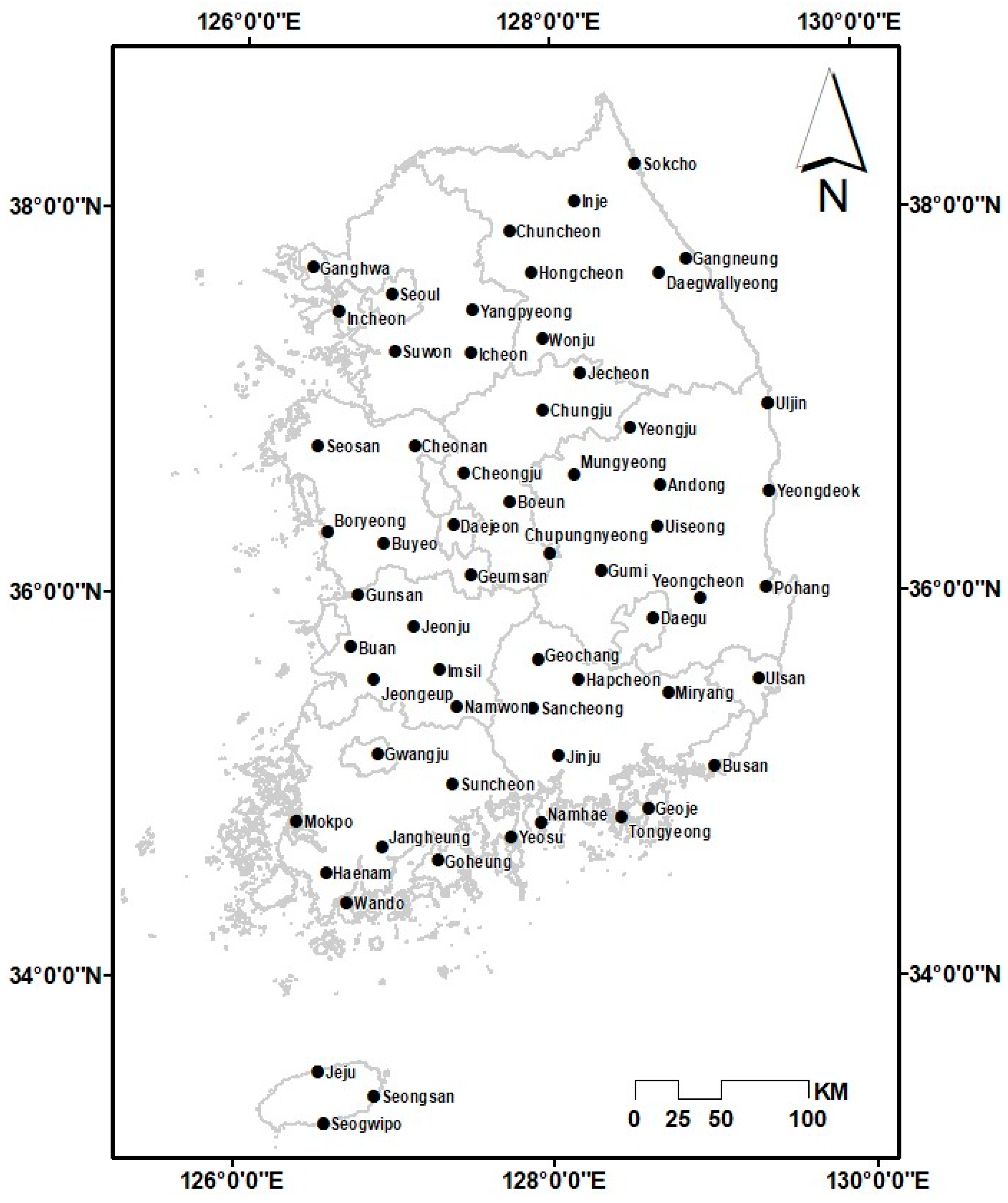
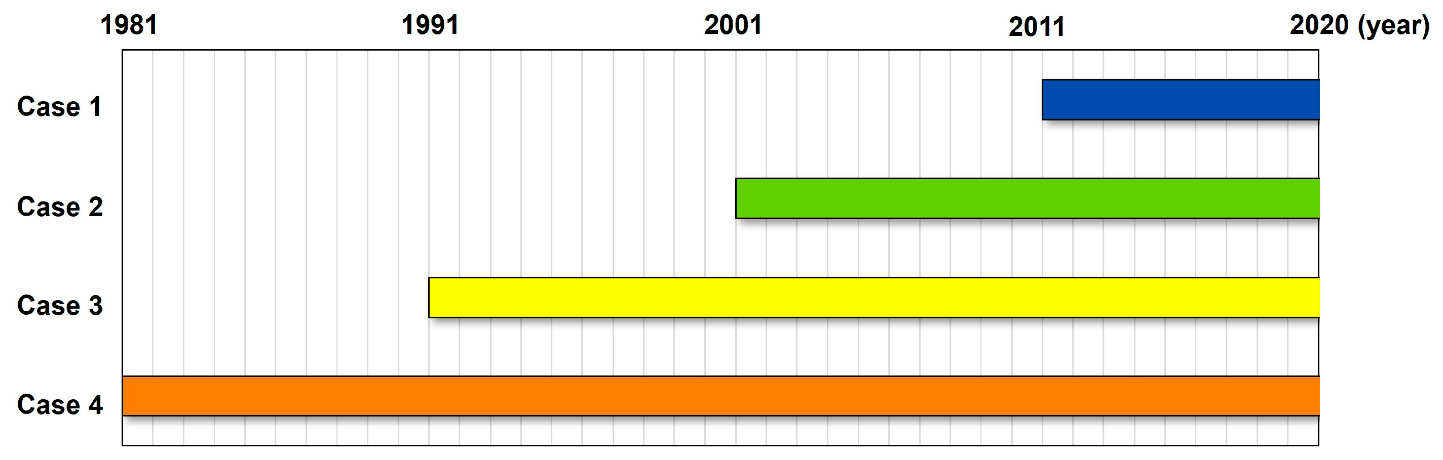
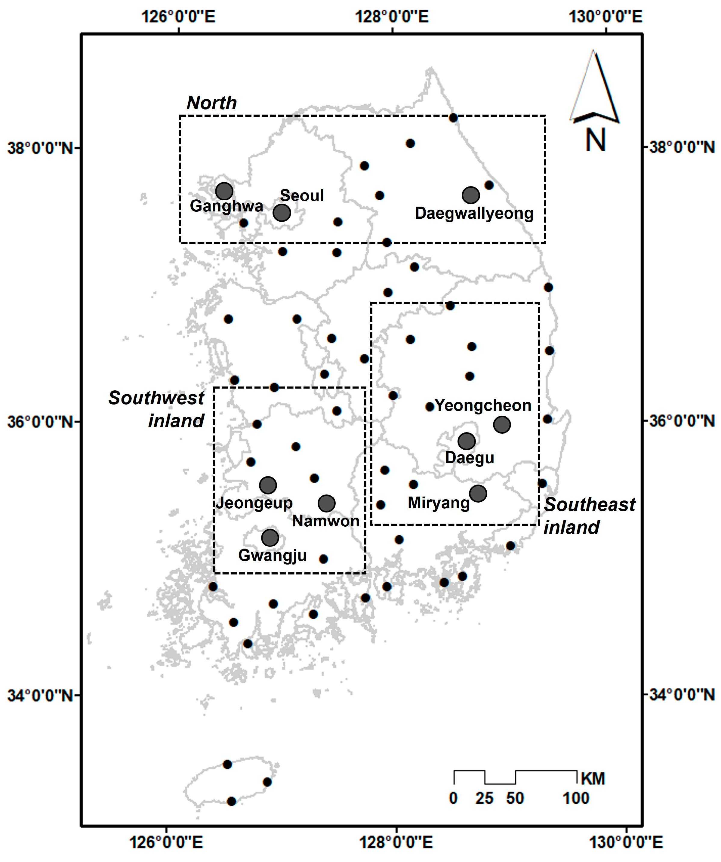
2.1. Rainfall Data

This study utilized hourly rainfall data from 61 stations in South Korea, as shown in Figure 1. For analyzing changes in rainfall patterns over time due to climate change, 61 stations with over 40 years of recorded data were selected from 102 Automated Synoptic Observing System (ASOS) stations. The ASOS rainfall data were obtained from the National Meteorological Data Center of the Korea Meteorological Administration.
This study conducted rainfall analysis for four different periods, i.e., 10, 20, 30, and 40 years starting from 2020, as shown in Figure 2.

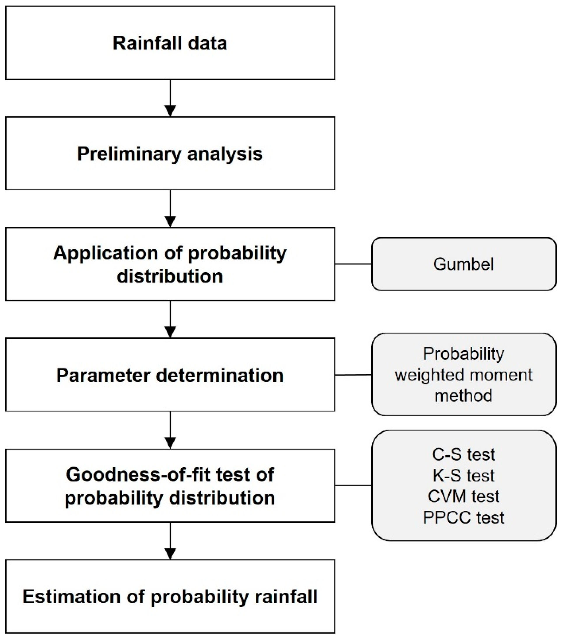
2.2. Estimation of Probability Rainfall

The probability rainfall was determined through a frequency analysis of rainfall data as depicted in Figure 3.
The annual maximum rainfall data series used for frequency analysis must exhibit independence. An independence test was performed as a preliminary check, employing three test methods: Anderson Correlation Test, Run Test, and Spearman’s Rank Correlation Coefficient Test. The results confirmed data independence by station, thus allowing for the application of the Gumbel distribution, a recommended probability distribution for all stations of the Korea Meteorological Administration, according to the Korean Design Rainfall Maps [40], for hydrological analysis. To estimate the probability distribution parameters, the probability-weighted moment method proposed by Greenwood [41] was used. This method yields relatively stable results even when the sample data are distorted by assigning smaller weights to lower values and larger weights to higher values. To determine the possibility of using the probability distribution, this study applied goodness-of-fit tests. Four goodness-of-fit tests were conducted for a significance level of α = 0.05, including the chi-square (C-S) test, Kolmogorov–Smirnov (K-S) test, Cramér–von Mises (CVM) test, and Probability Plot Correlation Coefficient (PPCC) test. These four tests quantitatively assess the fit between the data and the theoretical probability distribution based on the significance level. It was confirmed that the Gumbel distribution was suitable as it passed at least two of these test methods at all stations (Appendix A, Table A1 and Table A2). The probability density function (PDF) of the Gumbel distribution is as follows:
f x = 1 σ exp x μ σ exp x μ σ
where σ is a scale parameter, and μ is a location parameter. The cumulative probability density function (CDF) is the integral of PDF and has a probability value between 0 and 1. The CDF of the Gumbel distribution is as follows:
F x = exp exp x μ σ
The probability rainfall corresponding to the return period was obtained from the PDF. The frequency factor K T formula is an expression of the relationship between a PDF and the return period. The probability rainfall is estimated using the frequency factor K T and basic statistical values (mean and variance) of the probability distribution. In this study, we obtained the frequency factor for the 10-, 20-, 50-, and 100-year return periods. The probability rainfall for durations of 1, 2, 6, and 24 h was determined for each return period. The frequency factor formula of the Gumbel distribution and probability rainfall function [42] are as follows:
K T = 6 π 0.5772 + ln ln T T 1
x T = x ¯ + s K T
where x ¯ and s are the mean and standard deviation of x for each duration.

2.3. Intensity–Duration–Frequency (IDF) Curves

Rainfall intensity was calculated by dividing the probability rainfall by the duration. The IDF curve illustrates the relationship between rainfall intensity and duration for each return period. The regression equation of the IDF curve is called the intensity formula, which is used in various hydrological fields to plan infrastructure. In this study, the IDF parameters were estimated using the least-squares method, and the polynomial equation [43] expressed in Equation (5) was adopted as the formula for rainfall intensity.
ln I = a + b ln t + c ln t 2 + d ln t 3 + e ln t 4 + f ln t 5 + g ln t 6
where t is rainfall duration (hr), I is rainfall intensity (mm/h) according to rainfall duration, and a to g are local parameters.
The process of calculating rainfall intensity and duration using Equation (5) is described below in detail.
  • For the return period T n ( n = 10, 20, 50, and 100 years), the probability rainfall P n , i ˙ corresponding to the duration t i ( i = 1, 2, 6, and 24 h) is obtained. For example, when the return period is 50 years ( T 50 ), according to the duration 1 h ( t 1 ), 2 h ( t 2 ), 6 h ( t 6 ), and 24 h ( t 24 ), the probability rainfalls ( P 50 , 1 , P 50 , 2 , P 50 , 6 , and P 50 , 24 ) are calculated.
  • The rainfall intensity, I n , i is calculated by dividing the probability rainfall by the duration. For example, I 50 , 2 = P 50 , 2 t 2 .
  • Determine parameters a ,   b ,   c ,   d ,   e ,   f , and g for each T n by applying I n , i and t i to a polynomial equation. Since we consider four types of return period T n (10, 20, 50, and 100 years), we obtain four parameter sets of each return period in each station.
  • To know the specific condition I for mapping, the required return period T * and duration t * are fixed from a polynomial equation obtained in step III, and the rainfall intensity I * is calculated.
  • In the same way as step IV, T * * , and I * * are fixed, and t * * is obtained.

2.4. Kriging for Spatial Analysis

Many studies have combined dynamic and statistical approaches to downscale and perform the spatial interpolation of precipitation [34,44,45,46,47]. In this study, the probability rainfall data were recorded for 61 stations, along with the latitude and longitudinal coordinates of each station. We utilized ArcGIS 10.4 (ESRI) to map probability rainfall information, including rainfall intensity and duration, for each return period to visualize regional outcomes. The kriging interpolation tool in ArcGIS was used to create a raster layer with a 1 km resolution, consistent with the resolution applied in previous studies in South Korea [48,49,50]. The tool was used to weight the surrounding measured values and estimate values in unmeasured locations using the ArcGIS kriging function [47].

3. Results

Figure 4 illustrates the spatial distribution of annual average rainfall depth across four different rainfall period cases. Overall, the spatial distribution of annual rainfall depth appears similar in all four cases. However, Case 1 exhibits a distinct spatial pattern of annual rainfall depth distribution in the northern regions compared to Cases 2, 3, and 4. With the exception of the northern region, Case 1 closely aligns with the spatial distribution of annual rainfall depth in the other cases.

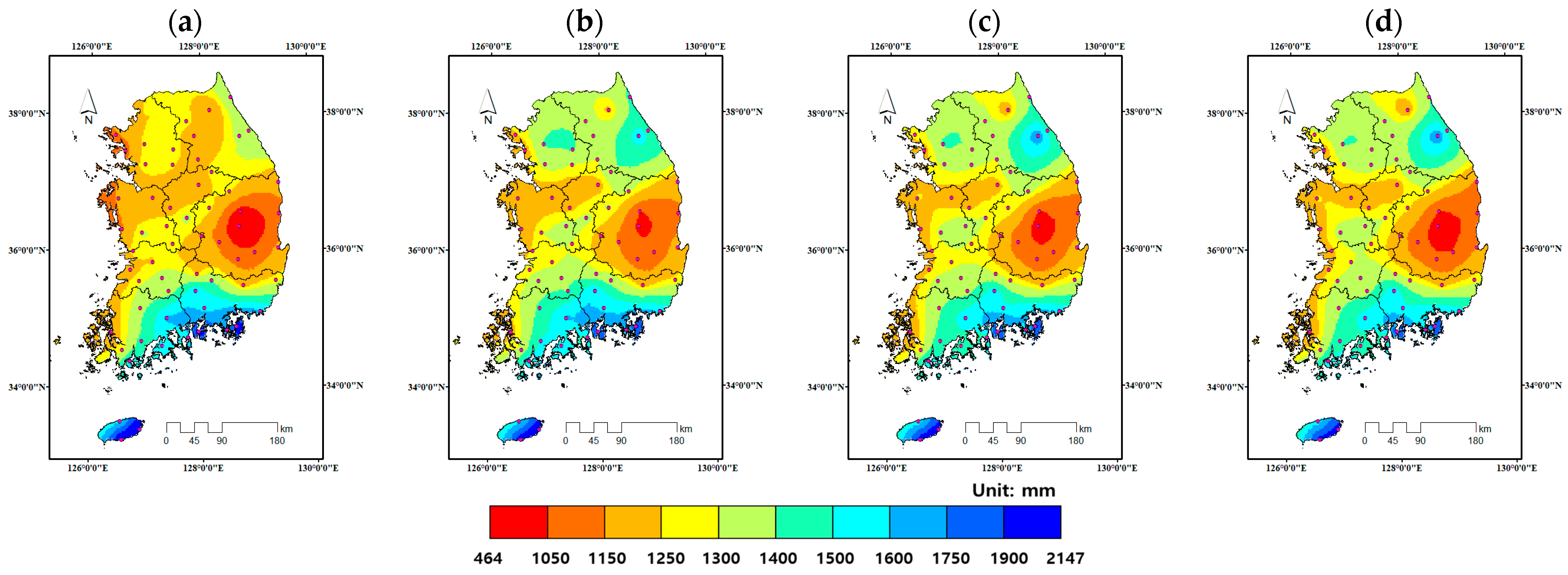
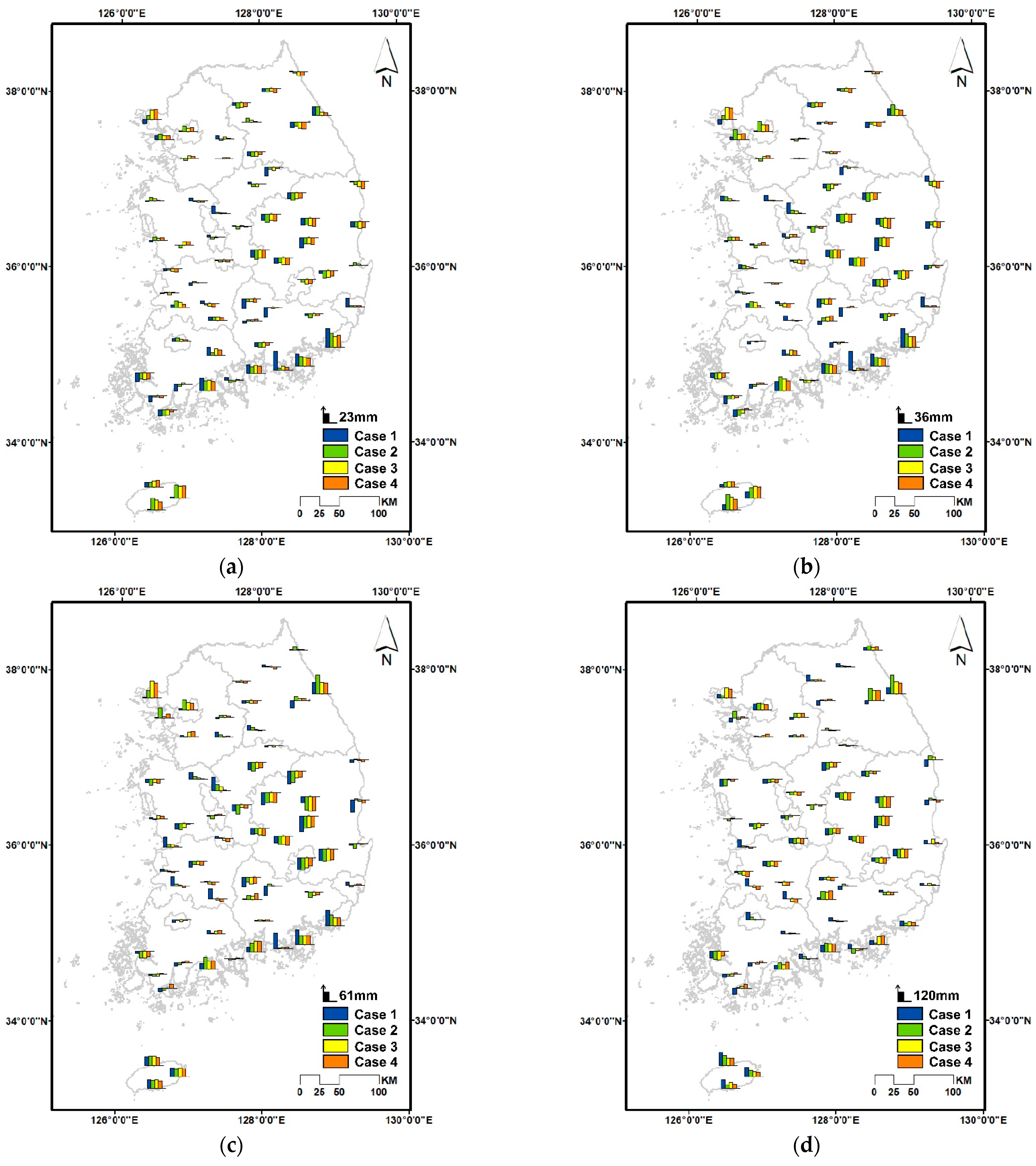
3.1. Spatial Distribution of Probability Rainfall with Consistent Rainfall Durations

Figures S1–S4 show the spatial distributions of probability rainfall based on constant rainfall durations (1, 2, 6, and 24 h) depending on different rainfall periods (Cases 1–4) and return periods (10, 20, 50, and 100 years). The deviation from the average of the probability rainfall was calculated to effectively identify the spatial change by case. Figure 5 shows the spatial distributions of probability rainfall anomalies averaged over four return periods. These anomalies are presented based on different rainfall durations and rainfall datasets, and each case is indicated in a different color. The bar chart on the map displays upward when the anomaly is positive (probability rainfall is greater than average) and downward when the anomaly is negative (probability rainfall is less than average). The larger the anomaly value (larger the difference from the average) the longer the bar chart is displayed, and the smaller the anomaly value (smaller the difference from the average) the shorter the bar chart is displayed. The scale bar at the bottom right of each map is the attribute value for chart symbols of that size. As shown in Figure 5, the scales of probability rainfall anomalies for different rainfall durations are 23 mm, 36 mm, 61 mm, and 120 mm, respectively. Generally, as rainfall durations increase, the scale of probability rainfall anomalies also rises. Across all combinations of return periods and rainfall data periods in Figure 5, the southeast inland region exhibits lower probability rainfall anomalies than other regions. Conversely, the northwest, northeast, and south coast regions consistently show higher probability rainfall anomalies than other regions. Notably, Jeju Island exhibits positive probability rainfall anomalies across all cases, primarily due to its higher annual average rainfall than that of the inland region (Figure 4).
Overall, certain regions exhibit distinct patterns of probability rainfall anomalies based on the rainfall dataset cases. Case 1, in particular, differs significantly from Cases 2, 3, and 4 in most regions, with coastal regions displaying notably contrasting patterns compared to inland regions between Case 1 and Cases 2–4. This suggests that Case 1 of the rainfall dataset characterizes significantly different patterns of probability rainfall anomalies from Cases 2–4, particularly in coastal regions.

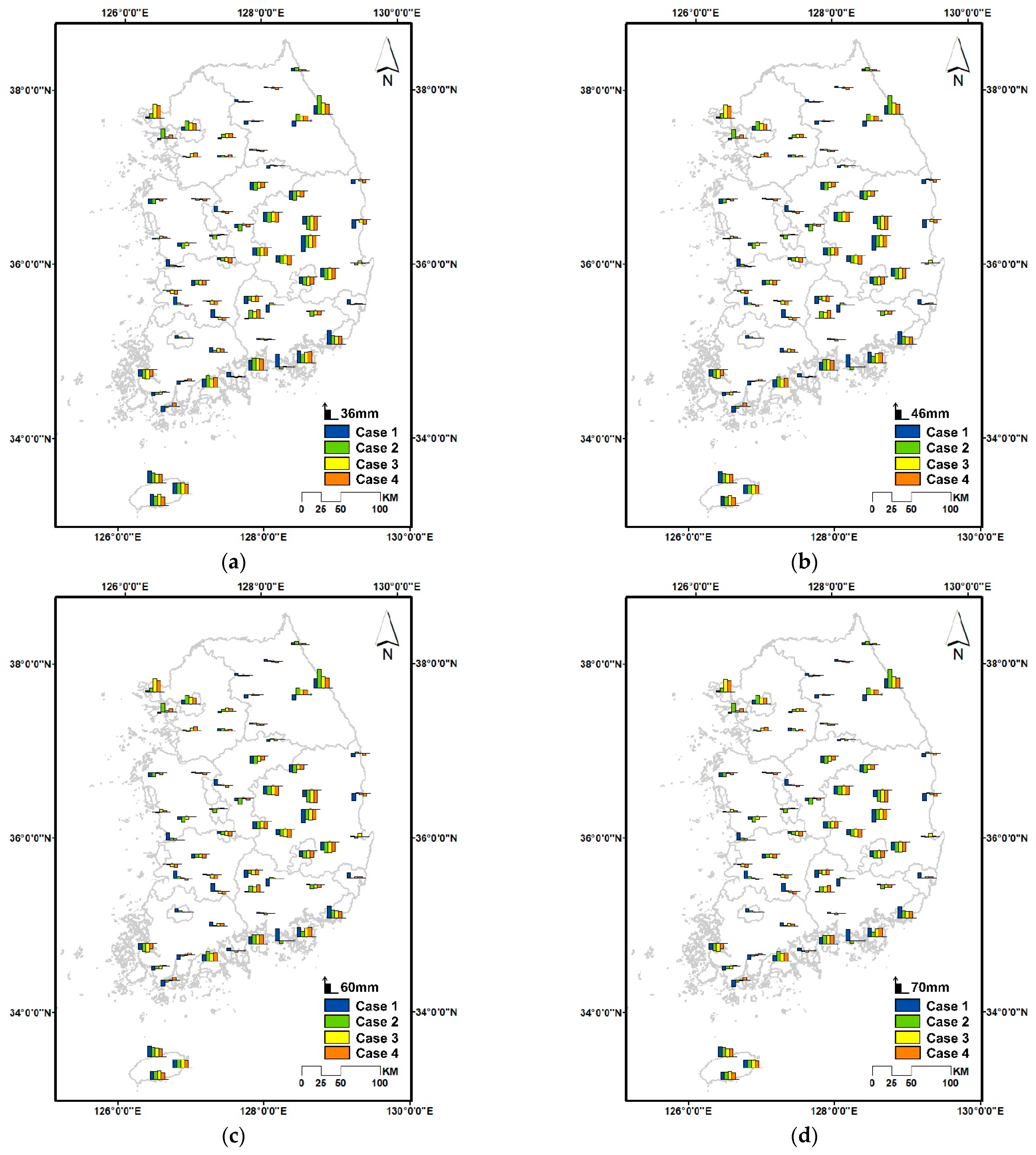
3.2. Spatial Distribution of Probability Rainfall with Consistent Rainfall Frequencies

Figures S5–S8 show the spatial distributions of the probability rainfall with constant 10-, 20-, 50-, and 100-year rainfall frequencies for different rainfall data periods (Cases 1–4) and rainfall durations (1, 2, 6, and 24 h). Figure 6 shows the spatial distributions of probability rainfall anomalies averaged over four durations, with four rainfall frequencies across different rainfall datasets. The scales of probability rainfall anomalies in Figure 6 are presented as 36 mm, 46 mm, 60 mm, and 70 mm, respectively. Notably, the scales of probability rainfall anomalies differ distinctly with varying return periods.
As shown in Figure 6, the northwest, northeast, and south coast regions exhibit positive probability rainfall anomalies, while the southeast inland region consistently displays negative probability rainfall anomalies. The spatial pattern of probability rainfall anomalies in Case 1 differs from Cases 2–4, but Cases 2–4 exhibit similar spatial distribution patterns among themselves. Specifically, Case 1 differs significantly from Cases 2–4 in the northwest, northeast, and southwest inland regions, while the southeast inland region demonstrates similar scales of probability rainfall anomalies across all rainfall periods.

3.3. Spatial Distribution of Probability Rainfall Intensity with Consistent Rainfall Durations

Figures S9–S12 show the spatial distributions of the probability rainfall intensity with constant 10-, 20-, 50-, and 100-year return periods depending on four different rainfall data periods (Cases 1–4) and four rainfall durations (1, 2, 6, and 24 h). Figure 7 shows the spatial distributions of probability rainfall intensity anomalies averaged across four return periods. These anomalies are presented for four rainfall durations and four different rainfall data periods. In Figure 7, the scales of probability rainfall intensity anomalies were large in short rainfall durations rather than long rainfall durations. For example, the scale of probability rainfall intensity anomalies in 1 h duration was approximately 23 mm/h, but about 5 mm/h for 24 h duration.
The probability rainfall intensity anomalies in the northwest, northeast, and south coast regions in Figure 7 are relatively higher than those in other regions. On the contrary, the southeast inland region consistently represents large negative probability rainfall anomalies across all rainfall periods. In 1-, 2-, and 6 h durations, Case 1 shows a different magnitude of probability rainfall anomalies compared to Cases 2, 3, and 4. However, for 24 h durations, Case 1 presents a similar magnitude of probability rainfall anomalies with other cases, in particular the south coast regions, indicating that longer duration provides a similar magnitude of probability rainfall anomalies.

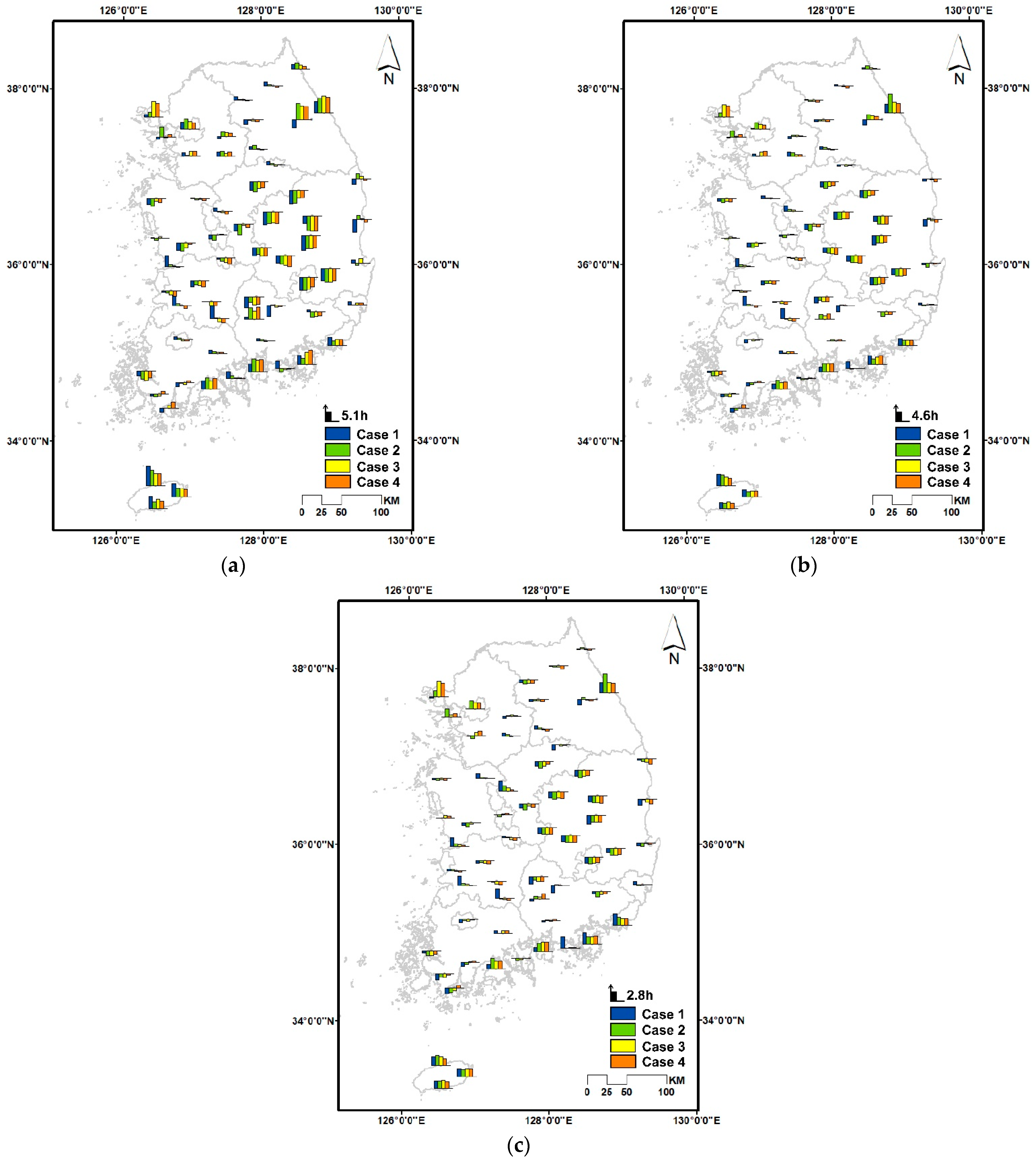
3.4. Spatial Distribution of Probability Rainfall Duration with Consistent Rainfall Intensities
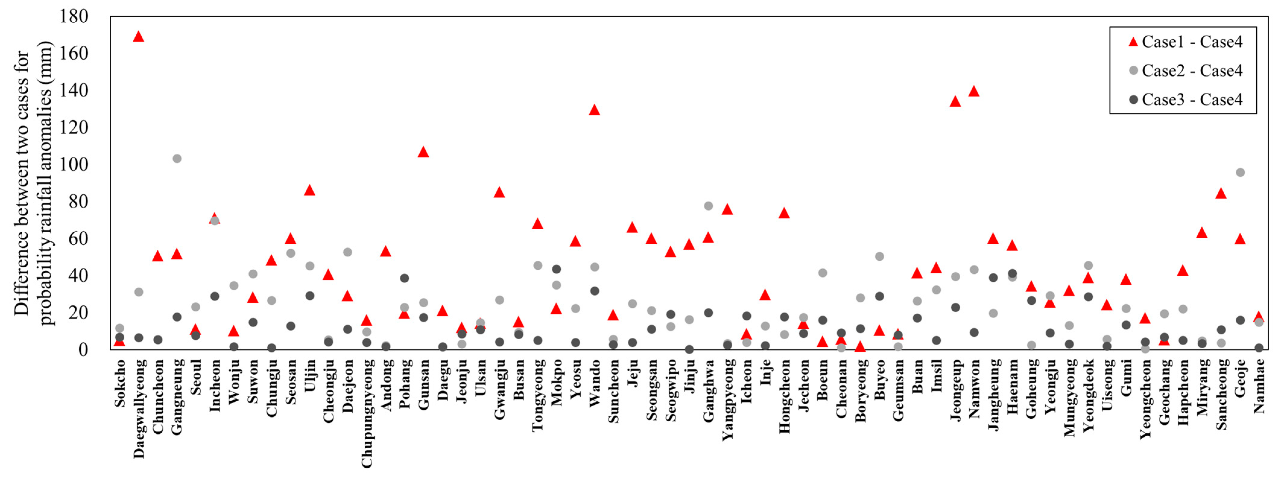
Figures S13–S16 show the spatial distributions of rainfall durations with constant 10-, 20-, 50-, and 100-year rainfall frequencies depending on the rainfall intensity (20, 30, and 40 mm/h) and rainfall data records (Cases 1–4). Figure 8 shows the spatial distributions of probability rainfall duration anomalies averaging four return periods. Spatial distributions of these anomalies are presented for constant rainfall intensities and four rainfall datasets. In Figure 8, the scale of probability rainfall duration anomalies is smaller as rainfall intensities increase. For example, for 20 mm/h, the scale of probability rainfall duration anomalies is about 5.1 h but is about 2.8 h for 40 mm/h. The low probability rainfall intensity of 20 mm/h in Figure 8a represents a greater spatial difference in rainfall duration anomalies than the high probability rainfall intensity of 40 mm/h in Figure 8c. This indicates that low rainfall intensity provides a large difference in the rainfall duration, and high rainfall intensity represents a small difference in rainfall duration.
In addition, the southwest inland and certain south coast regions exhibit distinct patterns of rainfall duration anomalies in Case 1 compared to other cases. For example, Case 1 portrays positive rainfall duration anomalies in the southwest inland region, whereas Cases 2, 3, and 4 display negative rainfall duration anomalies. This indicates that the rainfall patterns over the past 10 years (Case 1) differ from those observed over the past 20–40 years (Cases 2, 3, and 4), particularly in the southwest inland and some south coast regions.

4. Discussion

This study mapped and compared probability rainfall, rainfall intensity, and rainfall duration. Consistent with the rapid changes in rainfall volume and rainfall intensities over the past ten years mentioned in several studies [19,20,21], our study results also confirmed that the probability rainfall values change when data from the past 10 years are added. The results for Case 1 (2011–2020) showed clear differences when compared to the other cases. Figure 9 depicts the differences in probability rainfall anomalies of 24 h duration (Figure 5d) for Case 1, Case 2 (2001–2020), and Case 3 (1991–2020) relative to Case 4 which is the entire rainfall period (1981–2020). The difference between Case 1 and Case 4, indicated by a red triangle, is noticeably larger than the other cases. These results underscore significant differences in probability rainfall calculations when combining rainfall data for the last 10 years.
Moon et al. [37] classified 61 observation stations in South Korea into 10 regions and analyzed long-term precipitation data from 1980 to 2019. Precipitation variability exhibited different characteristics by region, with a slight increase of 4–12% in Gyeongsang-do and Jeju-do and a decrease of 2–9% in other regions. Zhou et al. [38] investigated changes in extreme precipitation events for 146 cities from 1960 to 2014, considering both climate change and urbanization. In the Jing-Jin-Ji (Beijing–Tianjin–Hebei) cluster, precipitation for all cities showed a decreasing trend, while cities in the Yangtze cluster experienced an increasing tendency. The impact of climate change differs regionally was also confirmed by this study’s results. We conducted mapping to assess spatial and temporal changes, revealing distinct regional effects. The difference in Case 1 compared to other rainfall periods is particularly evident in the northern and southwest inland regions. On the contrary, the southeast inland region showed similar results across all rainfall periods. The temporal and spatial effects of probability rainfall intensity and duration on the last 10 years of data were found to be similar to the probability rainfall results.
Therefore, in this study, we selected nine stations representing three regions to investigate temporal rainfall characteristics, aiming to understand the temporal variations of probability rainfall parameters such as return periods, rainfall intensity, and rainfall duration. These regions include Daegwallyeong, Ganghwa, and Seoul stations for the northern region; Gwangju, Jeongeup, and Namwon stations for the southwest inland region; and Daegu, Miryang, and Yeongcheon stations for the southeast inland region, as illustrated in Figure 10.
Figure 11 shows the box plots of decadal annual rainfall in nine representative stations. This figure clearly shows that the mean and box plots for the most recent 10 years (2011–2020) in Daegwallyeong, Ganghwa, Seoul, Gwangju, Jeongeup, and Namwon were remarkably lower than front decadal (2001–2010) box plots. However, for Daegu, Miryang, and Yeongcheon, the box plots for 2011–2020 closely resemble those of all other decades. This observation is further quantified in Table 1, which presents the average decadal rainfall for 2001–2010 and 2011–2020 by station, along with the absolute difference between these two averages. In the north and southwest inland regions, all absolute difference values exceed 115 mm, whereas in the southeast inland region, these values are 15 mm or less. The spatial patterns observed in the box plots for 2011–2020 compared to those for 1981–1990, 1991–2000, and 2001–2010 in Figure 11 align with the patterns characterizing different (Daegwallyeong, Ganghwa, Seoul, Gwangju, Jeongeup, and Namwon) or consistent (Daegu, Miryang, and Yeongcheon) probability rainfall factors across various rainfall periods. Figure 11 suggests a strong correlation between spatial patterns of probability rainfall, including return period, rainfall intensity, and rainfall duration, and changes in annual rainfall [51].

5. Conclusions

This study investigated the spatial distribution of probability rainfall, rainfall duration, rainfall frequency, and rainfall intensity in South Korea. To investigate the temporal effect, we applied four different rainfall data lengths: 2011–2020 (Case 1), 2001–2020 (Case 2), 1991–2020 (Case 3), and 1981–2020 (Case 4). The 61 rainfall stations were retrieved, and the Gumbel distribution was applied to estimate the probability rainfall in each station. Based on the results of this study, we mapped the combination of probability rainfall factors. In addition, anomalies, which are deviations from the average value, were mapped to compare changes in probability rainfall factors according to the rainfall data period setting. We found that the southeast inland region exhibited lower probabilities of rainfall, rainfall intensity, and duration compared to other areas, while the northeast, northwest, and south coast regions displayed higher probabilities of rainfall and rainfall intensity. Notably, we observed that as rainfall frequency decreased and duration increased, spatial differences in rainfall intensity and probability became more pronounced. In essence, the scales of probability rainfall and rainfall intensity increased with higher frequency and shorter duration, respectively.
For temporal analysis, Case 1 exhibited different results than other cases (Cases 2–4), showing that the spatial rainfall pattern of the recent 10 years differed from that of the past 40 years. This suggests that climate change has influenced the recent 10-year rainfall pattern in South Korea. In summary, our study underscores the divergence between recent and historical rainfall data in terms of spatial distribution. Furthermore, it confirms a strong correlation between annual rainfall and the temporal patterns of probability rainfall, rainfall intensity, rainfall durations, and return periods. The spatial and temporal distribution maps generated in this study are expected to serve as valuable resources for comprehending the spatial variations of probability rainfall variables, encompassing rainfall intensity, duration, and frequency, across various timeframes in South Korea. Finally, the spatial distribution maps provide important information for identifying flood-prone areas and establishing standards for the management and design of hydraulic structures.

Supplementary Materials

The following supporting information can be downloaded at: https://www.mdpi.com/article/10.3390/su152416646/s1, Figure S1. Spatial distribution of the 1 h rainfall probability based on different return periods and observed rainfall periods; Figure S2. Spatial distribution of the 2 h rainfall probability based on different return periods and observed rainfall periods; Figure S3. Spatial distribution of the 6 h rainfall probability based on different return periods and observed rainfall periods; Figure S4. Spatial distribution of the 24 h rainfall probability based on different return periods and observed rainfall periods; Figure S5. Spatial distribution of the 10 year return period based on different durations and observed rainfall periods; Figure S6. Spatial distribution of the 20 year return period based on different durations and observed rainfall periods; Figure S7. Spatial distribution of the 50 year return period based on different durations and observed rainfall periods; Figure S8. Spatial distribution of the 100 year return period based on different durations and observed rainfall periods; Figure S9. Spatial distribution of the rainfall intensity for a 10 year return period based on different durations and observed rainfall periods; Figure S10. Spatial distribution of the rainfall intensity for a 20 year return period based on different durations and observed rainfall periods; Figure S11. Spatial distribution of the rainfall intensity for a 50 year return period based on different durations and observed rainfall periods; Figure S12. Spatial distribution of the rainfall intensity for a 100 year return period based on different durations and observed rainfall periods; Figure S13. Spatial distribution of the rainfall duration for a 10 year return period based on different intensities and observed rainfall periods; Figure S14. Spatial distribution of the rainfall duration for a 20 year return period based on different intensities and observed rainfall periods; Figure S15. Spatial distribution of the rainfall duration for a 50 year return period based on different intensities and observed rainfall periods; Figure S16. Spatial distribution of the rainfall duration for a 100 year return period based on different intensities and observed rainfall periods.

Author Contributions

Conceptualization, M.L. and D.P.; methodology, M.L., H.A. and J.L.; formal analysis and investigation, M.-J.U., Y.J. and K.K.; resources, M.-J.U., Y.J. and K.K.; writing—original draft preparation, M.L. and H.A.; writing—review and editing, K.J. and S.K.; supervision, D.P.; funding acquisition, D.P. All authors have read and agreed to the published version of the manuscript.

Funding

This paper was supported by Konkuk University in 2022.

Institutional Review Board Statement

Not applicable.

Informed Consent Statement

Not applicable.

Data Availability Statement

The data presented in this study are available on request from the corresponding author.

Conflicts of Interest

Author Kewtae Kim is employed by ISAN Corporation. ISAN Corporation is not related to this research. The remaining authors declare that the research was conducted in the absence of any commercial or financial relationship that could be construed as a potential conflict of interest.

Appendix A

Table A1. Numbers given to 61 stations.
No.StationNo.StationNo.Station
1Sokcho21Gwangju41Buyeo
2Daegwallyeong22Busan42Geumsan
3Chuncheon23Tongyeong43Buan
4Gangneung24Mokpo44Imsil
5Seoul25Yeosu45Jeongeup
6Incheon26Wando46Namwon
7Wonju27Suncheon47Jangheung
8Suwon28Jeju48Haenam
9Chungju29Seongsan49Goheung
10Seosan30Seogwipo50Yeongju
11Uljin31Jinju51Mungyeong
12Cheongju32Ganghwa52Yeongdeok
13Daejeon33Yangpyeong53Uiseong
14Chupungnyeong34Icheon54Gumi
15Andong35Inje55Yeongcheon
16Pohang36Hongcheon56Geochang
17Gunsan37Jecheon57Hapcheon
18Daegu38Boeun58Miryang
19Jeonju39Cheonan59Sancheong
20Ulsan40Boryeong60Geoje
61Namhae
Table A2. Goodness-of-fit test results for Gumbel distribution for different durations and stations.
C-S Test
(Critical Value: 7.810)
K-S Test
(Critical Value: 0.210)
CVM Test
(Critical Value: 0.461)
PPCC Test
(Critical Value: 0.960)
Duration
1 h2 h6 h24 h1 h2 h6 h24 h1 h2 h6 h24 h1 h2 h6 h24 h
17.1007.1003.2002.9000.1150.1300.0870.0840.0890.0760.0700.0500.9870.9860.9830.980
24.4004.4004.4001.7000.0760.0970.1470.1030.0450.0450.1320.0680.9870.9840.9500.935
34.7001.1003.2003.2000.1100.0730.0600.1080.1320.0550.0410.0620.9670.9720.9890.984
46.80012.80020.3006.2000.1250.1510.1540.1240.1470.2170.2500.1030.9720.9750.9480.885
51.5853.0497.73210.0730.0850.0610.1010.1620.0750.0350.0560.1760.9830.9900.9900.979
62.6001.7007.4004.4000.1190.0560.1390.1020.0750.0280.1150.0650.9910.9830.9840.993
71.1008.0002.9001.1000.0810.1100.1220.0720.0750.1060.0850.0260.9900.9700.9800.996
82.6002.3009.8004.4000.0640.0920.1450.0860.0210.0430.2200.0670.9970.9880.9490.982
90.8002.3002.3003.2000.0570.0980.1050.1120.0310.0420.0620.0780.9930.9820.9880.984
102.0000.5001.7006.5000.0750.1050.0610.0800.0400.0450.0410.0580.9880.9890.9790.980
117.4004.7009.5003.5000.1040.1250.1900.0920.1100.0920.3140.0750.9100.9140.8430.914
124.4001.4009.2006.8000.1060.0690.1400.1060.1180.0330.1830.0740.9770.9820.9510.983
134.4002.0003.8001.7000.1220.0760.0830.0860.1180.0380.0560.0560.9510.9900.9880.986
149.8000.8000.5001.7000.0830.1090.0900.0970.1000.0730.0250.0420.9730.9890.9930.993
152.3005.3001.4002.6000.1150.0930.0810.0690.1100.0570.0570.0470.9790.9900.9340.985
164.1002.9002.0007.7000.1160.0950.1120.1530.1030.0910.1380.2270.9790.9620.9100.928
177.4004.40016.1007.7000.1050.1640.1310.1400.0880.1310.1770.1400.9880.9750.9660.979
180.5004.4002.6002.9000.0730.1090.0560.0710.0310.0670.0370.0430.9860.9750.9900.982
190.8001.7006.5000.5000.0780.0750.0930.0650.0280.0440.0720.0350.9950.9780.9840.986
202.9001.1001.7003.2000.0790.0850.0770.0780.0310.0380.0520.0450.9890.9700.9900.973
212.0005.30010.1009.8000.0650.1000.1370.1380.0180.0730.0960.1260.9950.9700.9700.953
223.8000.8002.6007.7000.0940.0620.0950.1070.0760.0220.0670.0890.9780.9860.9850.977
231.4001.7005.3004.7000.0720.0630.0810.1250.0390.0330.0570.0940.9920.9910.9710.974
242.9008.0002.3005.6000.1030.1010.1170.1500.1030.0980.0580.1150.9800.9800.9910.922
2512.2003.2008.0003.2000.1100.0730.1240.0940.1210.0580.0570.0590.9780.9720.9840.989
265.0007.7002.9008.9000.0830.1070.1160.1630.0410.0780.1030.2980.9910.9800.9800.958
275.9002.3007.4003.2000.1060.1090.0970.0790.0630.0710.0730.0590.9310.9840.9910.981
285.3000.8002.0000.8000.1160.0660.0850.0470.0490.0310.0670.0160.9900.9860.9840.994
292.0005.3005.6008.9000.0640.0950.0890.1090.0440.0640.0620.0910.9800.9660.9730.976
304.4001.7001.1001.7000.1060.0740.0710.0400.0630.0510.0220.0210.9760.9630.9960.990
314.4001.4006.2005.0000.1210.0770.1100.0960.1490.0340.0870.0540.9660.9830.9780.991
324.7004.1004.1002.3000.0860.1230.0700.0750.0460.0740.0340.0410.9820.9670.9440.967
333.5005.6004.1001.4000.0980.0860.0700.1030.0710.0870.0600.0670.9880.9810.9720.984
342.0007.7002.3004.1000.0590.0820.0860.1230.0430.0590.0450.0600.9870.9870.9820.991
355.3002.9002.0001.7000.1540.0960.0830.0580.1490.0930.0360.0320.9730.9580.9920.986
369.5003.8002.6002.9000.1230.0810.0650.0750.0990.0380.0550.0410.9880.9850.9740.991
371.1004.7004.1001.1000.0740.0570.0680.0750.0290.0290.0400.0420.9880.9950.9920.986
380.2002.6002.6005.0000.0730.0970.1420.1300.0270.0450.1550.0970.9880.9260.9110.973
394.4004.1002.0002.3000.0800.0710.0810.0700.0490.0360.0460.0400.9840.9900.9910.994
401.7000.8002.0005.6000.1060.0680.0810.1100.0640.0290.0430.1140.9890.9780.9820.981
414.4003.5004.1004.4000.0860.1310.1360.1080.0520.1160.1010.0930.9650.9440.9060.892
425.3002.6003.2004.4000.1220.0760.0780.0790.1180.0470.0420.1000.9760.9770.9820.968
438.3004.7005.9003.8000.1210.0990.0980.0980.0740.0830.0610.0480.9870.9820.9900.991
447.1001.7000.5008.6000.1350.0840.0670.0890.1660.0680.0290.0770.9650.9790.9930.976
452.3002.9003.2003.5000.0950.1110.1140.1210.0560.0900.1100.0880.9840.9740.9720.946
465.9002.9002.6004.7000.1090.1010.0540.0860.1060.0950.0330.0490.9810.9690.9920.970
472.6002.6006.8006.2000.0880.0740.0810.1730.0300.0380.0550.1820.9880.9930.9770.898
485.9002.9000.8002.6000.1560.0850.1010.0940.1020.0360.0400.0910.9830.9870.9910.960
492.3001.7000.8004.7000.0890.0770.1210.1210.0640.0420.0630.1270.9890.9870.9870.959
501.4000.2001.4000.8000.0530.0620.0730.0570.0240.0390.0360.0230.9960.9860.9870.985
514.1005.3003.8002.3000.0890.1080.0720.0770.1140.1640.0360.0420.9780.9780.9930.990
521.1004.4006.2005.6000.0750.1260.1640.1290.0450.1080.2510.2090.9940.9760.9540.965
533.2007.4001.4003.5000.0570.1310.0660.0970.0370.1430.0360.0960.9870.9750.9880.962
544.4008.0004.4001.4000.1330.0870.1240.0690.1230.0590.0920.0270.9770.9840.9870.981
558.6004.4005.9000.8000.1140.0770.1040.0910.0640.0510.0850.0630.9800.9950.9880.977
561.1003.2002.6003.5000.0680.0760.1050.0960.0580.0500.0520.0810.9830.9930.9890.984
572.3003.5003.2006.8000.0740.0780.0740.0930.0520.0670.0380.1050.9850.9760.9880.970
582.0002.9005.0003.2000.0710.0830.0720.0680.0640.0620.0380.0350.9850.9870.9880.986
591.1003.2005.0003.5000.0560.0730.1200.0770.0230.0390.1450.0760.9920.9910.9680.983
605.3004.7000.5007.7000.0820.0700.0450.1350.0750.0470.0290.1420.9810.9840.9930.965
613.5000.8001.4004.4000.0770.1290.0810.0930.0490.0800.0420.0680.9860.9880.9900.989
Note: The stations are indicated on the far left of the table with numbers specified in Table A1. The critical value of each goodness-of-fit test result at the 5% significance level of the Gumbel distribution is shown in parentheses. Statistically insignificant values are highlighted in bold letters on a red background.

References

  1. Korea Institute of Civil Engineering and Building Technology. A Planning Study on the Development of Safety Assessment System for Hydraulic Structures in Ungaged Basin; Korea Institute of Civil Engineering and Building Technology: Gyeonggi, Republic of Korea, 2018. [Google Scholar]
  2. Agilan, V.; Umamahesh, N.V.; Mujumdar, P.P. Influence of Threshold Selection in Modeling Peaks over Threshold Based Nonstationary Extreme Rainfall Series. J. Hydrol. 2021, 593, 125625. [Google Scholar] [CrossRef]
  3. Milly, P.C.; Betancourt, J.; Falkenmark, M.; Hirsch, R.M.; Kundzewicz, Z.W.; Lettenmaier, D.P.; Stouffer, R.J. Stationarity Is Dead: Whither Water Management? Science 2008, 319, 573–574. [Google Scholar] [CrossRef]
  4. Su, C.; Chen, X. Covariates for Nonstationary Modeling of Extreme Precipitation in the Pearl River Basin, China. Atmos. Res. 2019, 229, 224–239. [Google Scholar] [CrossRef]
  5. Um, M.-J.; Kim, Y.; Markus, M.; Wuebbles, D.J. Modeling Nonstationary Extreme Value Distributions with Nonlinear Functions: An Application Using Multiple Precipitation Projections for U.S. Cities. J. Hydrol. 2017, 552, 396–406. [Google Scholar] [CrossRef]
  6. Xu, P.; Wang, D.; Wang, Y.; Qiu, J.; Singh, V.P.; Ju, X.; Zhang, A.; Wu, J.; Zhang, C. Time-Varying Copula and Average Annual Reliability-Based Nonstationary Hazard Assessment of Extreme Rainfall Events. J. Hydrol. 2021, 603, 126792. [Google Scholar] [CrossRef]
  7. Yilmaz, A.G.; Hossain, I.; Perera, B.J.C. Effect of Climate Change and Variability on Extreme Rainfall Intensity–Frequency–Duration Relationships: A Case Study of Melbourne. Hydrol. Earth Syst. Sci. 2014, 18, 4065–4076. [Google Scholar] [CrossRef]
  8. Guo, B.; Zhang, J.; Meng, X.; Xu, T.; Song, Y. Long-Term Spatio-Temporal Precipitation Variations in China with Precipitation Surface Interpolated by ANUSPLIN. Sci. Rep. 2020, 10, 81. [Google Scholar] [CrossRef] [PubMed]
  9. Tabari, H. Climate Change Impact on Flood and Extreme Precipitation Increases with Water Availability. Sci. Rep. 2020, 10, 13768. [Google Scholar] [CrossRef]
  10. Trenberth, K.E.; Dai, A.; van der Schrier, G.; Jones, P.D.; Barichivich, J.; Briffa, K.R.; Sheffield, J. Global Warming and Changes in Drought. Nat. Clim. Chang. 2014, 4, 17–22. [Google Scholar] [CrossRef]
  11. Sarkar, S.; Maity, R. Increase in Probable Maximum Precipitation in a Changing Climate over India. J. Hydrol. 2020, 585, 124806. [Google Scholar] [CrossRef]
  12. Allan, R.P.; Soden, B.J. Atmospheric Warming and the Amplification of Precipitation Extremes. Science 2008, 321, 1481–1484. [Google Scholar] [CrossRef]
  13. Donat, M.G.; Lowry, A.L.; Alexander, L.V.; O’Gorman, P.A.; Maher, N. More Extreme Precipitation in the World’s Dry and Wet Regions. Nat. Clim. Chang. 2016, 6, 508–513. [Google Scholar] [CrossRef]
  14. Groisman, P.Y.; Knight, R.W.; Easterling, D.R.; Karl, T.R.; Hegerl, G.C.; Razuvaev, V.N. Trends in Intense Precipitation in the Climate Record. J. Clim. 2005, 18, 1326–1350. [Google Scholar] [CrossRef]
  15. Lee, T.; Son, C.; Kim, M.; Lee, S.; Yoon, S. Climate Change Adaptation to Extreme Rainfall Events on a Local Scale in Namyangju, South Korea. J. Hydrol. Eng. 2020, 25, 05020005. [Google Scholar] [CrossRef]
  16. Vu, T.M.; Mishra, A.K. Nonstationary Frequency Analysis of the Recent Extreme Precipitation Events in the United States. J. Hydrol. 2019, 575, 999–1010. [Google Scholar] [CrossRef]
  17. Utsumi, N.; Seto, S.; Kanae, S.; Maeda, E.E.; Oki, T. Does Higher Surface Temperature Intensify Extreme Precipitation? Geophys. Res. Lett. 2011, 38, GL048426. [Google Scholar] [CrossRef]
  18. Korea Meteorological Administration. Understanding of Climate Change and Application of Climate Change Scenarios; National Institute of Meteorological Research: Seoul, Republic of Korea, 2010. [Google Scholar]
  19. Kim, Y.-T.; Park, M.; Kwon, H.-H. Spatio-Temporal Summer Rainfall Pattern in 2020 from a Rainfall Frequency Perspective. J. Korean Soc. Disaster Secur. 2020, 13, 93–104. [Google Scholar]
  20. Kwon, H.-H.; Lall, U.; Kim, S.-J. The Unusual 2013–2015 Drought in South Korea in the Context of a Multicentury Precipitation Record: Inferences from a Nonstationary, Multivariate, Bayesian Copula Model. Geophys. Res. Lett. 2016, 43, 8534–8544. [Google Scholar] [CrossRef]
  21. Korea Meteorological Administration. Abnormal Climate Report in 2020; Office for Government Policy Coordination, Korea Meteorological Administration: Seoul, Republic of Korea, 2021. [Google Scholar]
  22. Nam, W.-H.; Hayes, M.J.; Svoboda, M.D.; Tadesse, T.; Wilhite, D.A. Drought Hazard Assessment in the Context of Climate Change for South Korea. Agric. Water Manag. 2015, 160, 106–117. [Google Scholar] [CrossRef]
  23. Im, E.S.; Jung, I.W.; Bae, D.H. The Temporal and Spatial Structures of Recent and Future Trends in Extreme Indices over Korea from a Regional Climate Projection. Int. J. Climatol. 2011, 31, 72–86. [Google Scholar] [CrossRef]
  24. Boo, K.-O.; Kwon, W.-T.; Baek, H.-J. Change of Extreme Events of Temperature and Precipitation over Korea Using Regional Projection of Future Climate Change. Geophys. Res. Lett. 2006, 33, GL023378. [Google Scholar] [CrossRef]
  25. Kim, G.; Cha, D.-H.; Park, C.; Lee, G.; Jin, C.-S.; Lee, D.-K.; Suh, M.-S.; Ahn, J.-B.; Min, S.-K.; Hong, S.-Y.; et al. Future Changes in Extreme Precipitation Indices over Korea. Int. J. Climatol. 2018, 38, e862–e874. [Google Scholar] [CrossRef]
  26. Jung, I.-W.; Bae, D.-H.; Kim, G. Recent Trends of Mean and Extreme Precipitation in Korea. Int. J. Climatol. 2011, 31, 359–370. [Google Scholar] [CrossRef]
  27. Jang, S.-W.; Seo, L.; Kim, T.-W.; Ahn, J.-H. Non-Stationary Rainfall Frequency Analysis Based on Residual Analysis. KSCE J. Civ. Environ. Eng. Res. 2011, 31, 449–457. [Google Scholar]
  28. Kwon, Y.-M.; Park, J.-W.; Kim, T.-W. Estimation of Design Rainfalls Considering an Increasing Trend in Rainfall Data. KSCE J. Civ. Environ. Eng. Res. 2009, 29, 131–139. [Google Scholar]
  29. Lee, C.; Ahn, J.; Kim, T. Evaluation of Probability Rainfalls Estimated from Non-Stationary Rainfall Frequency Analysis. J. Korea Water Resour. Assoc. 2010, 43, 187–199. [Google Scholar] [CrossRef]
  30. Ahn, J.-H.; Yoo, C.-S.; Yoon, Y.-N.; Kim, T.-W. Analysis of the Changes in Rainfall Quantile According to the Increase of Data Period. J. Korea Water Resour. Assoc. 2000, 33, 569–580. [Google Scholar]
  31. Oh, T.-S.; Kim, M.-S.; Moon, Y.-I.; Ahn, J.-H. An Analysis of the Characteristics in Design Rainfall According to the Data Periods. J. Korean Soc. Hazard Mitig. 2009, 9, 115–128. [Google Scholar]
  32. Ahmad, I.; Zhang, F.; Tayyab, M.; Anjum, M.N.; Zaman, M.; Liu, J.; Farid, H.U.; Saddique, Q. Spatiotemporal Analysis of Precipitation Variability in Annual, Seasonal and Extreme Values over Upper Indus River Basin. Atmos. Res. 2018, 213, 346–360. [Google Scholar] [CrossRef]
  33. Mishra, A.K.; Singh, V.P. Changes in Extreme Precipitation in Texas. J. Geophys. Res. Atmos. 2010, 115, jd013398. [Google Scholar] [CrossRef]
  34. Simonovic, S.P.; Schardong, A.; Sandink, D. Mapping Extreme Rainfall Statistics for Canada under Climate Change Using Updated Intensity-Duration-Frequency Curves. J. Water Resour. Plan. Manag. 2017, 143, 04016078. [Google Scholar] [CrossRef]
  35. Song, X.; Zhang, J.; Zou, X.; Zhang, C.; AghaKouchak, A.; Kong, F. Changes in Precipitation Extremes in the Beijing Metropolitan Area during 1960–2012. Atmos. Res. 2019, 222, 134–153. [Google Scholar] [CrossRef]
  36. Easterling, D.R.; Evans, J.L.; Groisman, P.Y.; Karl, T.R.; Kunkel, K.E.; Ambenje, P. Observed Variability and Trends in Extreme Climate Events: A Brief Review. Bull. Am. Meteorol. Soc. 2000, 81, 417–426. [Google Scholar] [CrossRef]
  37. Moon, J.; Shim, C.; Jung, O.; Hong, J.W.; Han, J.; Song, Y.I. Characteristics in Regional Climate Change over South Korea for Regional Climate Policy Measures: Based on Long-Term Observations. J. Clim. Chang. Res. 2020, 11, 755–770. [Google Scholar] [CrossRef]
  38. Zhou, X.; Bai, Z.; Yang, Y. Linking Trends in Urban Extreme Rainfall to Urban Flooding in China. Int. J. Climatol. 2017, 37, 4586–4593. [Google Scholar] [CrossRef]
  39. Ministry of Land Infrastructure and Transport. A Study on Improvement and Supplement of Probability Rainfall Map; Ministry of Land Infrastructure and Transport: Gyeonggi, Republic of Korea, 2011. [Google Scholar]
  40. Ministry of Construction and Transportation. Probability Rainfall Map in South Korea: Water Resources Management Technique Development Research Report; Ministry of Construction and Transportation: Seoul, Republic of Korea, 2000. [Google Scholar]
  41. Greenwood, J.A.; Landwehr, J.M.; Matalas, N.C.; Wallis, J.R. Probability Weighted Moments: Definition and Relation to Parameters of Several Distributions Expressable in Inverse Form. Water Resour. Res. 1979, 15, 1049–1054. [Google Scholar] [CrossRef]
  42. Ariff, N.M.; Jemain, A.A.; Ibrahim, K.; Zin, W.W. IDF Relationships Using Bivariate Copula for Storm Events in Peninsular Malaysia. J. Hydrol. 2012, 470, 158–171. [Google Scholar] [CrossRef]
  43. Pilgrim, D.H. Australian Rainfall and Runoff: A Guide to Flood Estimation; Institution of Engineers: Barton, Australia, 1987. [Google Scholar]
  44. Wu, T.; Li, Y. Spatial Interpolation of Temperature in the United States Using Residual Kriging. Appl. Geogr. 2013, 44, 112–120. [Google Scholar] [CrossRef]
  45. Paparrizos, S.; Maris, F.; Matzarakis, A. Integrated Analysis of Present and Future Responses of Precipitation over Selected Greek Areas with Different Climate Conditions. Atmos. Res. 2016, 169, 199–208. [Google Scholar] [CrossRef]
  46. Qi, B.; Liu, H.; Zhao, S.; Liu, B. Observed Precipitation Pattern Changes and Potential Runoff Generation Capacity from 1961–2016 in the Upper Reaches of the Hanjiang River Basin, China. Atmos. Res. 2021, 254, 105392. [Google Scholar] [CrossRef]
  47. Borchardt, S.; Choi, W.; Choi, J. Effects of Climate, Basin Characteristics, and High-Capacity Wells on Baseflow in the State of Wisconsin, United States. JAWRA J. Am. Water Resour. Assoc. 2022, 58, 135–148. [Google Scholar] [CrossRef]
  48. Ahn, S.-R.; Kim, S.-J. Assessment of Watershed Health, Vulnerability and Resilience for Determining Protection and Restoration Priorities. Environ. Model. Softw. 2019, 122, 103926. [Google Scholar] [CrossRef]
  49. Jung, C.; Lee, J.; Lee, Y.; Kim, S. Quantification of Stream Drying Phenomena Using Grid-Based Hydrological Modeling via Long-Term Data Mining throughout South Korea Including Ungauged Areas. Water 2019, 11, 477. [Google Scholar] [CrossRef]
  50. Park, J.; Kim, D.-S.; Song, K.H.; Jeong, T.-J.; Park, S.-J. Mapping Potential Habitats for the Management of Exportable Insects in South Korea. J. Asia-Pac. Biodivers. 2018, 11, 11–20. [Google Scholar] [CrossRef]
  51. Wallis, J.R.; Schaefer, M.G.; Barker, B.L.; Taylor, G.H. Regional Precipitation-Frequency Analysis and Spatial Mapping for 24-Hour and 2-Hour Durations for Washington State. Hydrol. Earth Syst. Sci. 2007, 11, 415–442. [Google Scholar] [CrossRef]
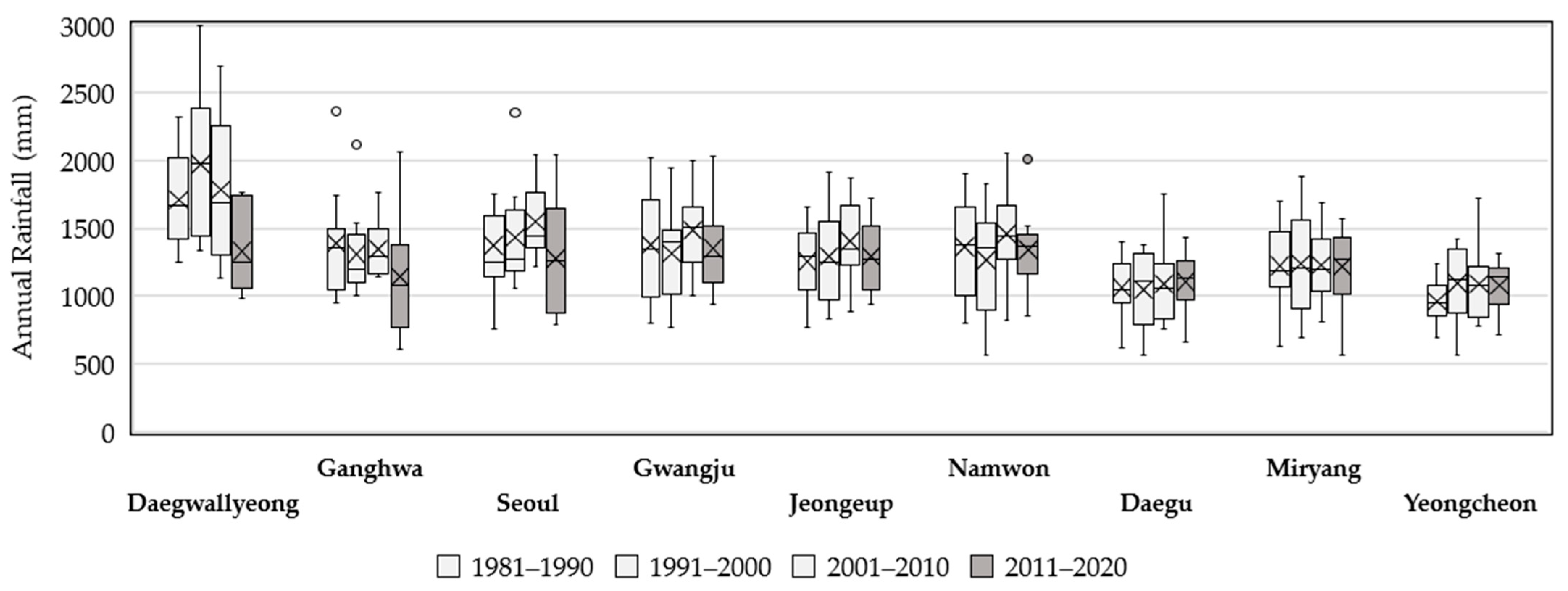
Figure 1. Study area.
Sustainability 15 16646 g001
Figure 2. Four analysis periods for frequency analysis.
Sustainability 15 16646 g002
Figure 3. Frequency analysis procedure for probability rainfall estimation [39].
Sustainability 15 16646 g003
Figure 4. Spatial distribution of annual average rainfall depth for different rainfall return periods: (a) Case 1; (b) Case 2; (c) Case 3; and (d) Case 4.
Sustainability 15 16646 g004
Figure 5. Frequency mean anomalies of probability rainfall for different durations: (a) 1 h; (b) 2 h; (c) 6 h; and (d) 24 h.
Sustainability 15 16646 g005
Figure 6. Mean anomalies of probability rainfall for different return periods: (a) 10-year; (b) 20-year; (c) 50-year; and (d) 100-year.
Sustainability 15 16646 g006
Figure 7. Frequency mean anomalies of probability rainfall intensity for different durations: (a) 1 h; (b) 2 h; (c) 6 h; and (d) 24 h.
Sustainability 15 16646 g007
Figure 8. Frequency mean anomalies of probability rainfall duration for different rainfall intensities: (a) 20 mm/h; (b) 30 mm/h; and (c) 40 mm/h.
Sustainability 15 16646 g008
Figure 9. Difference between two cases for probability rainfall anomalies (mean frequency and 24 h duration) for 61 stations.
Sustainability 15 16646 g009
Figure 10. Selected stations for annual rainfall analysis.
Sustainability 15 16646 g010
Figure 11. Box plots of four decadal annual rainfall in nine representative stations.
Sustainability 15 16646 g011
Table 1. Average decadal rainfall by station (2001–2010 and 2011–2020) and the absolute difference in average decadal rainfall by period.
RegionStationAverage Decadal Rainfall (mm)
(2001–2010)
Average Decadal Rainfall (mm)
(2011–2020)
Absolute Difference *,
(mm)
NorthDaegwallyeong1782.31329.1453.2
Ganghwa1345.21141.9203.4
Seoul1550.21274.2275.9
Southwest inlandGwangju1482.41352.2130.2
Jeongeup1403.51290.1113.4
Namwon1455.71339.9115.8
Southeast inlandDaegu1088.01102.714.7
Miryang1226.61214.512.1
Yeongcheon1088.61075.613.0
* Absolute differences in average decadal rainfall for 2001–2010 and 2011–2020.
Disclaimer/Publisher’s Note: The statements, opinions and data contained in all publications are solely those of the individual author(s) and contributor(s) and not of MDPI and/or the editor(s). MDPI and/or the editor(s) disclaim responsibility for any injury to people or property resulting from any ideas, methods, instructions or products referred to in the content.

