

Recharge Estimation Approach in a Data-Scarce Semi-Arid Region, Northern Ethiopian Rift Valley
by
 ,
,
Sisay S. Mekonen
1,2,*,
Scott E. Boyce
1,3 ,
,
Abdella K. Mohammed
4,
Lorraine Flint
5,
Alan Flint
5 and
Markus Disse
1
1
Chair of Hydrology and River Basin Management, School of Engineering and Design, Technical University of Munich, 80333 Munich, Germany
2
Faculty of Water Resources and Irrigation Engineering, Arba Minch University, Arba Minch P.O. Box 21, Ethiopia
3
U.S. Geological Survey, California Water Science Center, 4165 Spruance Rd., Suite 200, San Diego, CA 92101-0812, USA
4
Faculty of Hydraulic and Water Resources Engineering, Arba Minch University, Arba Minch P.O. Box 21, Ethiopia
5
Earth Knowledge Inc., Tucson, AZ 85751-0743, USA
*
Author to whom correspondence should be addressed.
Sustainability 2023, 15(22), 15887; https://doi.org/10.3390/su152215887
Submission received: 10 October 2023
/
Revised: 2 November 2023
/
Accepted: 8 November 2023
/
Published: 13 November 2023
/
Corrected: 22 March 2024
(This article belongs to the Special Issue Groundwater Hydrology, Contamination, and Sustainable Development)
Abstract
:Sustainable management of groundwater resources highly relies on the accurate estimation of recharge. However, accurate recharge estimation is a challenge, especially in data-scarce regions, as the existing models are data-intensive and require extensive parameterization. This study developed a process-based hydrologic model combining local and remotely sensed data for characterizing recharge in data-limited regions using a Basin Characterization Model (BCM). This study was conducted in Raya and Kobo Valleys, a semi-arid region in Northern Ethiopia, considering both the structural basin and the surrounding mountainous recharge areas. Climatic Research Unit monthly datasets for 1991 to 2020 and WaPOR actual evapotranspiration data were used. The model results show that the average annual recharge and surface runoff from 1991 to 2020 were 73 mm and 167 mm, respectively, with a substantial portion contributed along the front of the mountainous parts of the study area. The mountainous recharge occurred along and above the valleys as mountain-block and mountain-front recharge. The long-term estimates of the monthly recharge time series indicated that the water balance components follow the temporal pattern of rainfall amount. However, the relation of recharge to precipitation was nonlinearly related, showing the episodic nature of recharge in semi-arid regions. This study informed the spatial and temporal distribution of recharge and runoff hydrologic variables at fine spatial scales for each grid cell, allowing results to be summarized for various planning units, including farmlands. One third of the precipitation in the drainage basin becomes recharge and runoff, while the remaining is lost through evapotranspiration. The current study’s findings are vital for developing plans for sustainable management of water resources in semi-arid regions. Also, monthly groundwater withdrawals for agriculture should be regulated in relation to spatial and temporal recharge patterns. We conclude that combining scarce local data with global datasets and tools is a useful approach for estimating recharge to manage groundwater resources in data-scarce regions.
1. Introduction
Water scarcity is increasingly becoming a monumental challenge, particularly in arid and semi-arid regions, where the water supply primarily comes from groundwater sources, as surface water sources are inadequate and unreliable [1,2,3,4]. In these areas, especially in rapidly expanding urban and agricultural regions, sustainable groundwater resource development and management rely on reliable estimates of recharge and its variability in time and space [5,6,7,8,9,10]. Accurately estimating recharge is one of the most challenging water-balance components as it is highly spatially and temporally variable and is affected by many factors (e.g., climate, topography, vegetation, soil, and geology) [11,12,13,14,15,16].
Many studies have developed approaches for recharge estimations at different scales [17]. However, the reliability of the methods depends on many factors such as catchment characteristics, availability, and accuracy of field data [18]. While most methods fail to accurately estimate the recharge, they do not account for spatial and temporal variability [14]. Recharge rates and distributions are difficult to directly quantify and costly to measure over larger spatial scales [15,16]. Hydrologic models are becoming more popular and widely used for estimating recharge; however, they are data-intensive and require extensive parameterization and detailed hydroclimate and hydrogeological data [14,18,19,20]. Additionally, most of the hydrologic models rely on water balance in some capacity, fail to account for bedrock properties, and overlook the influence of spatially varying bedrock conductivity on recharge estimates [21]. Other approaches that explicitly account for the influence of bedrock conductivity are two- and three-dimensional finite-element (FE) numerical models, although the computational requirements in the models covering small areas limit their applicability [22,23,24].
Another method that balances the numerical computational burden with the accuracy of the simulation by refining water balance components while accounting for bedrock permeability is the Basin Characterization Model (BCM). The BCM was developed by Flint and Flint [13] at the U.S. Geological Survey (USGS). The BCM is a physically-based gridded regional water-balance model that considers aquifer bedrock properties and vegetation-specific actual evapotranspiration to estimate recharge and runoff [13,21,24,25]. The model is superior to other watershed models as it spatially characterizes the amount of water that infiltrates below the root zone at a rate corresponding to bedrock conductivity that can become groundwater recharge [26,27]. To this end, the BCM has been successfully applied to reliably estimate recharge and runoff in many parts of the world, for example, in California and Western United States [12,26,28,29,30]. The recharge and runoff components have also been used as boundary conditions for numerous groundwater flow models and software [31,32,33,34,35,36]. In addition, the model is used for a variety of applications, including the evaluation of the effects of urbanization, wildfire, and forest management on hydrology [37,38]; the evaluation of the effects of soil management on recharge, climatic water deficit, and forage production [39,40]; and the modeling of future climate projections to evaluate water availability [27,41].
Recent advancements in fine-scale modeling enable the creation of models for landscape-scale planning for decision making in agriculture and ecosystems [21,42,43]. The BCM has the capacity to execute hydrologic variables at fine spatial grid resolution to quantify hydrologic dynamics at scales computationally prohibitive to capture the dynamics of the water balance components. This enabled the BCM to reliably estimate recharge by using fine-scale data that reflect landscape heterogeneity and complexity. Fine-scale data allow for the consideration of the greater spatial and temporal distribution of recharge estimates [44,45], which increases the accuracy of contaminant transport and groundwater flow models [46]. For example, a study by Ackerly and Loarie [47] used PRISM data at 4 km to plan conservation, examine the difference compared to the fine-scale spatial heterogeneity using a model of climatic impacts at 30 m, and find that a fine-scale process captures topographic variability and corresponding variations in air temperature, providing information and better interpretation for conservation planning. Similar studies by [26] and Thorne and Boynton [29,30,48] used the BCM with a spatial resolution of 270 m × 270 m to estimate recharge and assess the magnitude and spatial patterns of historical and future hydrologic changes in California watersheds, and they found that a finer spatial resolution is important to quantify hydrologic dynamics at scales applicable to hydrologic modeling for regional landscape applications.
The current study developed a reliable approach for estimating recharge by refining water balance components and using finer-resolution input data (10 m by 10 m) by combining local data with global datasets in a data-scarce semi-arid region. The BCM is capable of executing hydrologic variables at a finer spatial grid resolution to reliably quantify recharge as it captures spatial heterogeneity and complexity. A two-step calibration approach was applied to improve the recharge estimate: first, to vegetation-specific actual evapotranspiration and the underlying bedrock properties, and second, to the observed streamflow gauge. The results of this study can be used as input boundary conditions to a three-dimensional groundwater flow model to support groundwater management decisions for future sustainable groundwater development and use. This study’s findings will also help guide recharge estimation by combining local data with global datasets and tools to manage groundwater resources in data-limited regions.
2. Materials and Methods
2.1. Study Area
2.1.1. Location, Topography, and Slope
The Raya and Kobo Valleys are located in the Afar Depression, the western edge of Ethiopia’s main rift valley, the Great Rift Valley in East Africa. The study area lies between 11.92° and 12.90° N and 39.30° and 39.90° E and consists of two valleys, Raya Valley in Tigray Region and Kobo Valley in Amhara Region (Figure 1). It covers an area of 3506 km2 with elevation ranging from 1018 m above mean sea level in the valley plain to 3948 m above mean sea level on the top of the mountain. The study area is characterized by a hilly topography and has slopes ranging from 2% in the valley plain to 75% in the mountainous areas.
The valley’s residents have access to surface water and groundwater to meet the water needs of the valley. The increasing population and agricultural growth have increased water demand in the valley. The surface water system is ephemeral and prone to water shortages during drought. To ensure a stable water supply, the Raya and Kobo Valleys’ community relies on groundwater as the primary water source for domestic water supply and agricultural irrigation. Increasing water demand in the Raya and Kobo Valleys has led to an expansion of groundwater use without proper management of groundwater resources [49].
2.1.2. Geology or Geomorphology
The East African Great Rift System is a place where the final stages of a continental breakup are observed and actively deforming [50]. Because of its location, the valley is geologically complex in structure, stratigraphy, and lithology. The formation of the geologic structure is controlled by tectonic events that led to the development of the rift system and is characterized by normal faults and a series of marginal grabens that formed the valley floor [51]. These marginal grabens are narrow and elongated depressions bounded on either side by opposing normal faults. Tectonic evolution has formed mountain ranges that bound the marginal grabens on the western and eastern sides. The framework runs north–south, through the valley on the west and the ridge on the east. The valley is predominantly alluvial, composed of deposits of sand, gravel, boulders, clay, and volcanic rocks underlain by Mesozoic limestone (Figure 2). The study area typically consists of two principal geomorphic features: mountain terrain and lower valley floors of the alluvial plains.
2.1.3. Water Resources
The groundwater basin, the lower elevation zones, are characterized by a semi-arid climate. The topography affects both precipitation and temperature. Precipitation is generally higher in the mountains and lower on valley floors, whereas temperature is warmer on valley floors and cooler in the mountains. The study area’s rainfall pattern is bimodal, with the main rain occurring in the summer from June to September and with the highest rainfall recorded in July and August. In this study, June, July, August, and September—the main rainy months—are considered as wet seasons, and the remaining months are considered as dry seasons. The mean annual rainfall of the study area based on two met stations in the valley is 668 mm, whereas it is 927 mm based on three stations in the highlands. The average monthly temperature of the study area ranges from 17 °C to 26 °C in the valley and 12 °C to 17.5 °C in the highland areas.
2.2. Datasets
2.2.1. Observed Data
Soil data from two sources were used. The Ethiopian Construction Design & Supervision Works Corporation office (WCDSWC) contains 1-to-50,000-scale soil data for the Kobo and Raya Valleys. We combined the WCDSWC map with the national soil database developed by the Ethiopian Ministry of Agriculture (MoA). Using the combined soil maps, we identified six main soil types in the drainage basin (Figure 3a). The valley area is primarily covered by silty clay and black clay soil types. The western, mountainous parts of the drainage basin are primarily loam, sandy loam, and loamy sand soil types. We also developed a land use map from the MoA national digital soil map. This map identified six major land use types: crops, shrubland, trees, water area, bare land, and developed-built areas. The land use of the study area is dominated by crops and shrubland (Figure 3b).
Maximum and minimum temperatures, precipitation, wind speed, relative humidity, and sunshine duration data were collected from Ethiopia’s National Meteorological Agency (NMA) (http://www.ethiomet.gov.et/). The datasets (2000–2015) were obtained from five meteorology stations distributed across the study area. Historical stream gauge data were obtained from two gauging stations from 1985 to 2005. Following the data quality assessment, one stream gauging station was found reliable and used for model calibration and validation.
2.2.2. Climate Datasets
Precipitation and maximum and minimum air temperature from the Climatic Research Unit (CRU 4.05; [52]) transient monthly dataset (1991–2020) of 40 km native resolution were downscaled to 10 m for our model consumption. CRU datasets are known for their higher temporal resolution, and since the first release in 2000, they have been widely utilized by many users in diverse research areas and applications [42,52,53].
The spatial downscaling was performed on the 40 km data grids to 1 km grids by the USGS team, and then the methods described in Flint and Flint [26] were used to produce finer-resolution grids of 10 m by 10 m. This approach uses gradient-plus-inverse-distance squared interpolation (GIDS) [54]. GIDS combines the location and elevation of the new finer-resolution grid relative to the existing coarse-resolution grid cells for parameter weighting; it is shown to not introduce additional uncertainty in the downscaling process and, instead, improves the estimate of the climate parameter by taking into consideration the deterministic influence of location and elevation on climate [26]. The downscaled grid data are then bias-corrected using regression coefficients generated from meteorological data of the study area using the Bouwer and Aerts [55] method, applied and described in detail [26,56].
Potential evapotranspiration (PET) was calculated using the modified Priestley–Taylor equation [57], which considers topographic shading, cloud cover, and vegetation density. The method helps to look at where the sun is relative to the slope and consider the effects of ridges that would block the sun during any part of the day. This is the step at which detailed information about the geospatial layers is considered to improve the characterization of landscape processes.
There were no field observations of actual evapotranspiration (AET) data for the study area. As a surrogate for AET, remotely sensed data were used. Remote-sensing-based AET estimates from the Moderate-Resolution Imaging Spectrometer (MOD16 AET) and the Food and Agricultural Organization of the United Nations (FAO) portal (water productivity open access portal, WaPOR) have been widely used as options to calibrate and validate hydrologic models in Ethiopia [58,59,60,61] and other countries [62,63]. For this study, we used WaPOR as it offers continuous actual evapotranspiration data across Africa and the Middle East at three spatial resolutions (250 m, 100 m, and 30 m). The quality of the WaPOR dataset was evaluated across Africa and resulted in enough quality to contribute to the understanding and monitoring of local and continental water processes and water management [58]. WaPOR would suit many users’ needs due to the low biases and good spatial variability across Africa. Due to the limited AET data availability across Africa, the reliability of nine remote-sensing-derived evapotranspiration products was evaluated by [64] at the basin scale using the water balance approach, and WaPOR was among the three recommended to users due to the low biases and good spatial variability across Africa. Chukalla and Mul [65], in their work on irrigation performance assessment for sugarcane estates in Mozambique, tested WaPOR data and recommended it because the datasets can be presented as a substitute choice that offers a significant benefit, particularly in regions where there are limited in situ data. As a result of the elevation variation from 1018 m in the valley plain to 3948 m above mean sea level on the top of the mountain, distinct variations in AET were observed in the study area (Figure 4). The average AET was used to develop monthly vegetation parameters (Kv) for model calibration to match the modeled AET to estimates that have been developed using remotely sensed observations.
2.3. Methodology
2.3.1. General
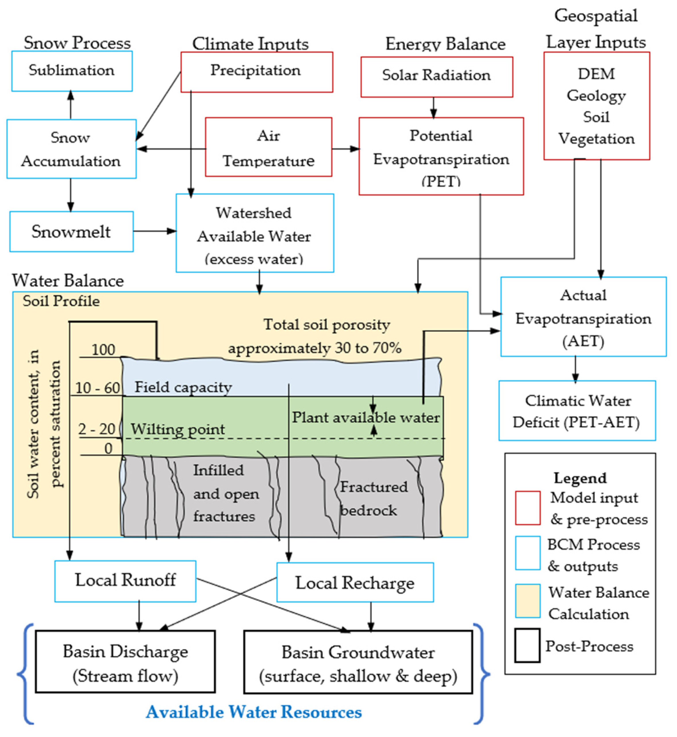
The current study used BCM, a monthly, gridded, regional water-balance model, to estimate recharge and runoff using soils, geology, topography, and transient monthly maps of precipitation, air temperature, and potential evapotranspiration datasets. The model is locally calibrated and simulated for 1991 to 2020 water years. Generally, the methodology consists of three processing steps (Figure 5): pre-processing, model run, and post-processing. Fortran codes and QGIS 3.2 software [66] were used to pre-process the input files, run the model, and summarize and perform analysis of BCM outputs.
Climate data (precipitation and air temperature), potential evapotranspiration, geospatial layers (geology, soils, and vegetation), and the DEM of the study area were assembled. All input climate grids and maps of the property layers were prepared at the same 10 m × 10 m grid scale for the operation of the model. The model simulation, including water balance calculation, was performed in the second step. The model combined spatially distributed climate data and monthly PET data along with the DEM, bedrock conductivity (Ks), soil properties (water content at field capacity and wilting point, soil depth, porosity, and soil hydraulic conductivity), and simulated recharge and runoff maps along with time series of monthly and yearly outputs. The BCM only simulated vertical flows, and the lateral flow simulations were separately performed using an Excel spreadsheet in step three, the post-processing step. In this step, runoff, baseflow, and recharge calculations were performed from BCM recharge and runoff simulation output maps using equations that combine recharge and runoff using scaling parameters and exponential functions to match measured hydrographs. A detailed description of the BCM post-processing equations can be found in Flint and Flint [13].
2.3.2. Description of the Basin Characterization Model (BCM)
BCM is a water balance model that runs using Fortran code and relies on monthly time series of spatially distributed climate parameters input files, including potential evapotranspiration, spatially distributed properties of soils, and geologic property layer files and control files for model parameterization (Figure 5). All input files (Table 1) are in ASCII text format and have the same grid scale, dimension, and map projection, similar to the digital elevation model (DEM). The BCM control file (Appendix A) contains input and output file names, LOOKUP tables of vegetation for density and growth parameters, hydraulic conductivity corresponding to the geologic unit identification for each bedrock geologic type, and the period for the model simulation (1991–2020). The main output files generated by BCM simulations include monthly gridded maps of output variables for excess water, actual evapotranspiration, soil-water storage, climatic water deficit, recharge, runoff, and monthly and yearly output files that include time series for the simulation period.
In the BCM, the water balance conceptual model considers unimpaired conditions and solves the following equation in the monthly time step: precipitation—evapotranspiration—sublimation—runoff—recharge—change in soil storage = 0. In this study, the snow process, one of the components of the BCM, was not considered, as the study area is in a semi-arid climatic region, and no snow was observed. The BCM begins with precipitation and air temperature input followed by the calculation of PET from solar radiation with topographic shading and cloudiness. Then, gridded PET, precipitation, and maximum and minimum air temperature are used to produce available excess water. The excess water provides the water available in the watershed for water balance calculation (Figure 5). This excess water occupies the soil profile and, depending on the soil properties and conductivity of the underlying bedrock, it becomes either recharge or runoff. Generally, BCM simulates what moves below the root zone that has the potential to become groundwater recharge. In wetter regions, it may return to streams as baseflow, while in arid regions with losing streams, it may move downward through the unsaturated zone. The thickness and porosity of the unsaturated zone will dictate when and if the recharge reaches the aquifer.
The excess water that exceeds the total soil storage (porosity) becomes runoff, or, if it is less than porosity but greater than field capacity, it percolates through the soil profile to become recharge at the rate of bedrock conductivity on a monthly time step. The water less than field capacity will be calculated as actual evapotranspiration at the rate of PET until it reaches the wilting point. Then, runoff and recharge are combined to calculate basin discharge in post-processing and calibrated to the measured stream flows. The climate water deficit, the evaporative demand that exceeds the available water, is calculated by subtracting the actual evapotranspiration from PET. The model calculates hydrologic variables on a grid cell basis and runs the model at a fine spatial resolution of 10 m by 10 m. The fine resolution enables the capture of the dynamics of the water balance components that contributes to the reliable recharge estimation.
2.4. Model Performance Evaluation
An antecedent condition switch was used to initialize the model run, and the calibration period covered 13 years (1984–1996), with wet, normal, and dry years observed over this period. Six parameters were calibrated manually: LAI (leaf area index to allow for calculations of vegetation density variables that are used to change the sensitivity to match the measured data), UpRate and DnRate (variables used to determine how quickly vegetation grows back from a disturbance at a rate controlled by the amount of precipitation for that month), UpLimit and DnLimit (parameters within which the maximum yearly LAI can vary as a result of the variability of climate), and RootDepth (allows the depth of soil to be increased to simulate the storage of water below the mapped soil depth). Initially, the default values were adopted from [13] and changed as necessary to achieve the desired calibration results (Appendix B).
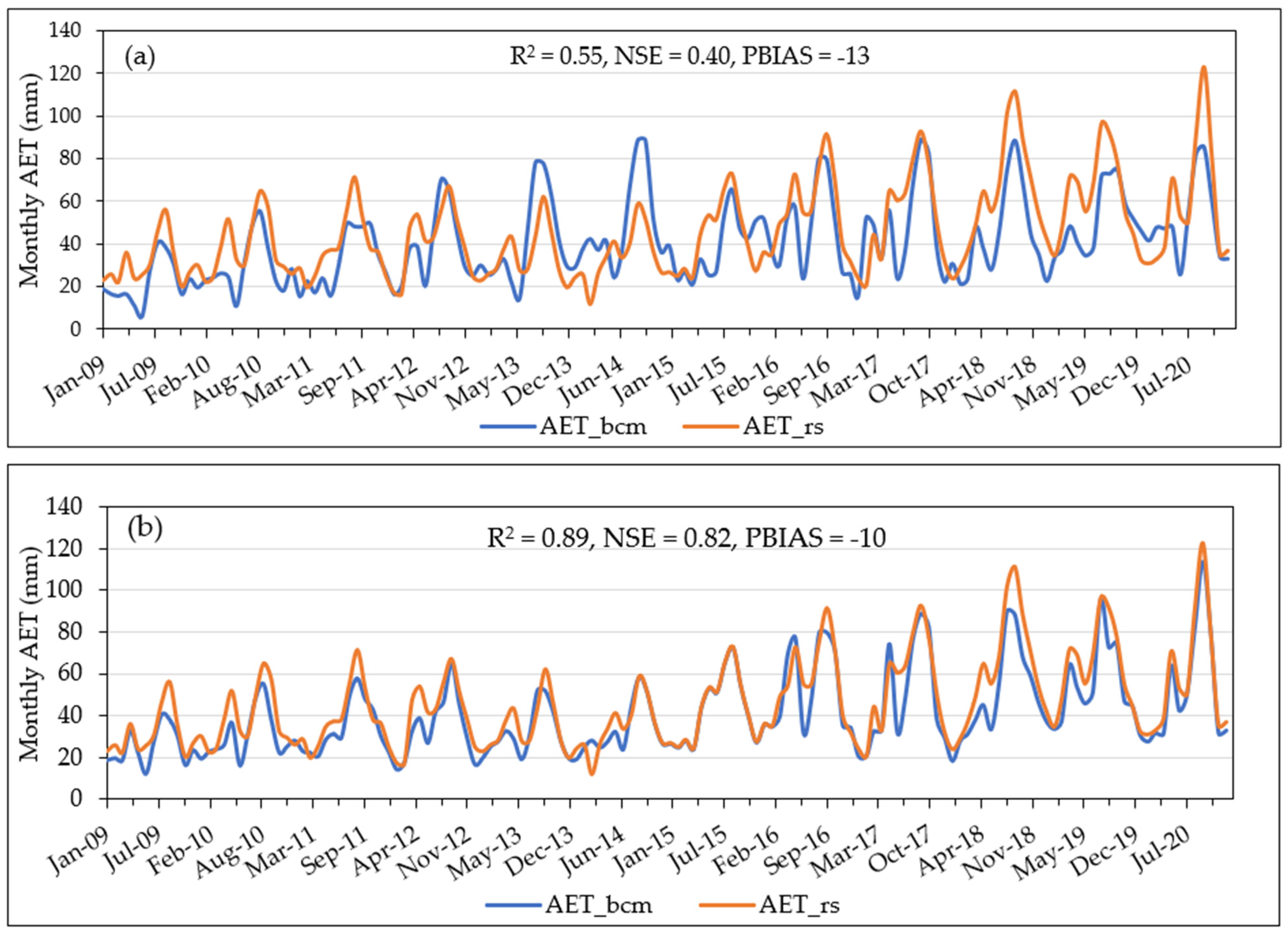
BCM calibration started by calibrating AET to match the available data. Monthly vegetation parameters (Kv) were developed based on the actual evapotranspiration (AET_rs) ratio from remotely sensed data to the average monthly time series of PET for the period of the record generated from the BCM for each vegetation type. These Kv values were used for the BCM to calculate the actual evapotranspiration (AET_bcm) to be compared with AET_rs. The calibration parameters, vegetation density and growth parameters, were iteratively adjusted to optimize the agreement of the AET of the BCM with the AET of remote sensing data. The initial and final values of the vegetation density and growth parameters used in this study are listed in Appendix B.
The estimate of basin discharge as a time series requires further calculation as BCM calculates recharge and runoff for every grid cell. The BCM recharge and runoff are calibrated using a post-processing calculation and the observed streamflow gauges. Calibration was performed by adjusting the net conductivity of bedrock and coarse alluvium values. The values were iteratively adjusted to alter the proportion of excess water that becomes recharge and runoff for optimizing the match between the calculated basin discharge and measured streamflow.
BCM model results are for unimpaired stream flows. An unimpaired stream flow represents natural hydrologic flow conditions where water is not diverted from nor supplied to a basin, for example, due to agricultural or municipal diversions. The unimpaired recharge and runoff from the watershed upstream of the gauges are calculated by summing the BCM grid cell values upstream of the gauging station. The total upstream, unimpaired flow is compared to the measured stream gauge using post-processing equations. This BCM recharge and runoff calibration process is performed by considering equations for in-stream gains and losses, including base flow, seepage, and deep flow to the aquifer, by adjusting coefficients (scaling factors and exponents), explained in detail [13]. Then, an independent five-year dataset (1997–2001) was used to validate the model.
The model was then assessed for performance using three goodness-of-fit statistics: Nash–Sutcliffe Efficiency (NSE), Coefficient of Determination (R2), and Percent Bias (PBIAS). Nash–Sutcliffe efficiency [67] measures the match between the simulated and observed stream flow pattern and is widely used to evaluate the performance of hydrologic models. The Coefficient of Determination (R2) is the measure of collinearity between simulated and measured data [68] and is suggested as a useful comparative statistic by [69]. Percent Bias (PBIAS) estimates the percentage trend of simulated data to be greater or smaller than the observed data [70]. The equations for the three goodness-of-fit statistics are
where Qsim is the simulated streamflow; Qobs is the observed streamflow (m3/s); the overbar symbol denotes the mean of the observed and simulated streamflow values; i is the time step (monthly); and n is the number of days of the simulation period.
The calibrated BCM model was then used to simulate recharge and runoff as gridded maps for the simulation period (1991–2020). The analysis then focused on the long-term trends of recharge as a monthly, seasonal, and yearly average, for the thirty-year simulation period.
3. Results and Discussion
3.1. BCM Calibration and Validation
For calibration of AET, vegetation parameters are developed and calibrated using the actual evapotranspiration of remote sensing (AET_rs) and modeled actual evapotranspiration from BCM (AET_bcm). The time series of monthly AET_rs data and AET_bcm values calculated with the BCM for the calibration period (2009–2020) were plotted and showed good agreement with adjusted model parameters (Figure 6). Vegetation parameters were used to adjust the AET_bcm to match based on the sensitivity to changes in annual precipitation. Figure 6b shows monthly AET for 2009–2020 with AET_bcm matched to AET_rs. The BCM underestimated most peaks but well captured the trend and the magnitude of AET compared to the remote sensing data. Figure 6 reveals the validity of the water balance component estimates with growth parameter adjustment compared with no parameter adjustment. AET remote sensing data can be considered as an alternative in the absence of measured data.
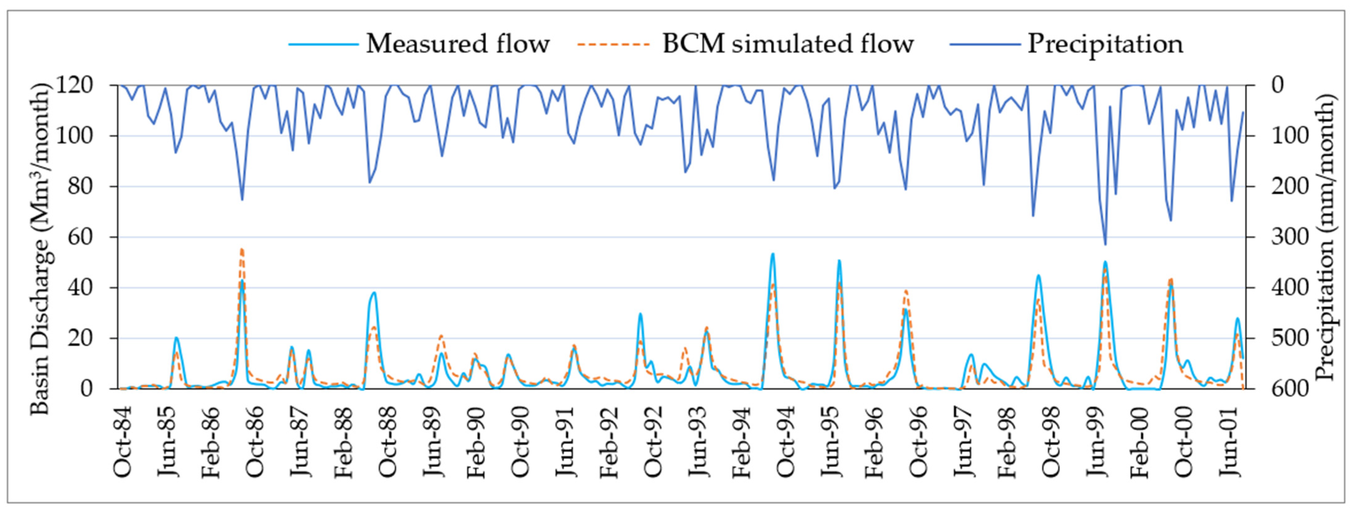
Calibration of the BCM recharge and runoff to measured streamflow was performed by plotting streamflow data from the Golina gauging station against BCM simulated streamflow and precipitation. We used the Golina sub-basin, for which the bedrock conductivity corresponding to the geologic types located within the subbasin was iteratively changed to alter the proportion of excess water that becomes recharge or runoff to optimize the match between the simulated sub-basin discharge and measured streamflow. The initial and calibrated values of the Ks are given in Appendix C. The model was calibrated for twelve years (1985–1996) and validated for five years (1997–2001) (Figure 7). The gauging station used for calibration has no impairments, increasing the model’s performance as BCM produces unimpaired runoff. Then, the model’s performance was evaluated using the previously defined goodness-of-fit statistics (Table 2).
NSE values for the monthly streamflow calibration and validation are 0.78 and 0.75, respectively. According to the model performance ratings’ recommended statistics for a monthly time step, BCM simulated the streamflow trends very well, as shown by the statistical results, which agree with the graphical results. The R2 values are 0.83 and 0.78 for both calibration and validation, respectively, which indicates that the model performance for streamflow residual variation showed very good performance. The PBIAS values showed 2.28% during calibration and 8.34% during validation. The magnitude of simulated monthly streamflow values was within the very good range (PBIAS < ±10) for calibration and validation. Generally, the model showed a good performance with values slightly higher for calibration than validation. The overall performance revealed that the model could be considered for analyzing historical and future hydrological changes (recharge and runoff estimation). The calibration and validation performance indicates that the model can be locally calibrated for smaller watersheds, increasing the model’s performance as watershed impairments can be easily assessed and evaluated.
3.2. Recharge and Runoff Estimates
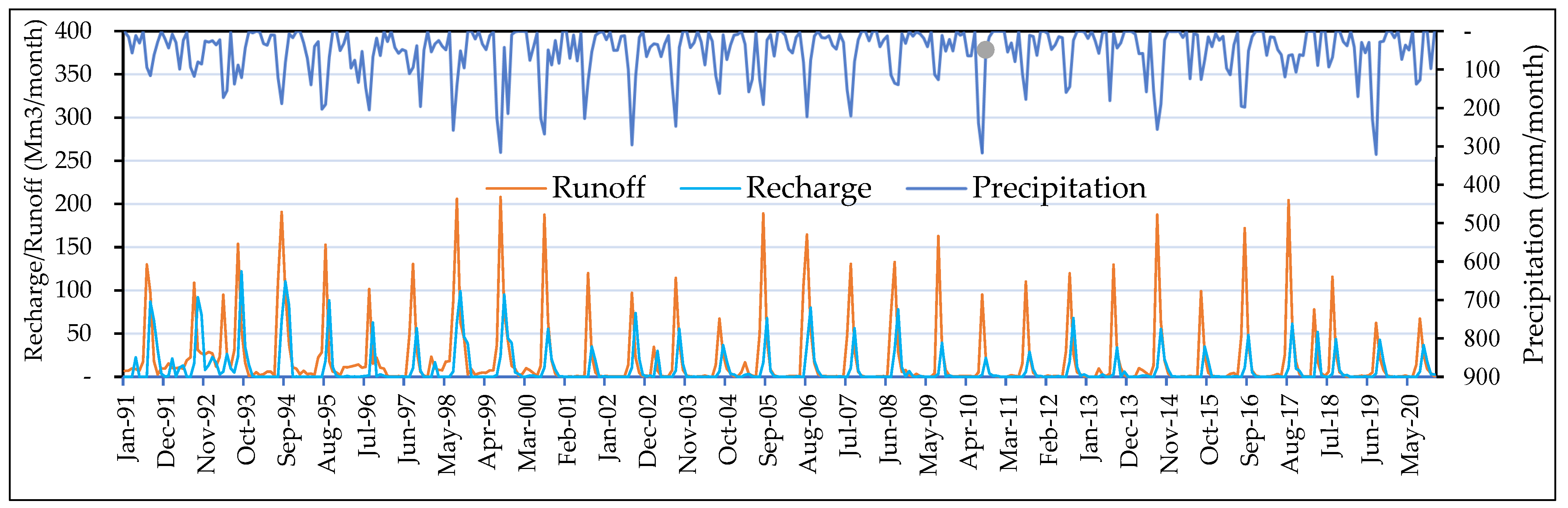
This study analyzed the generated in-place recharge and runoff output through BCM simulations as gridded maps and monthly and yearly time series outputs of the long-term trends for the simulation period (1991–2020). The long-term estimates of monthly recharge and runoff time series were computed over the entire catchment area of 3506 km2 at a horizontal grid resolution of 10 m by 10 m (Figure 8). The modeling results show that recharge and runoff in the study area are temporally variable. The estimated recharge is generally lower than the estimated runoff. The estimated monthly recharge (1991 to 2020) ranges from zero to 126.22 × 10⁶ m3, while the runoff ranges from 2.04 × 10⁶ m3 to 295.56 × 10⁶ m3.
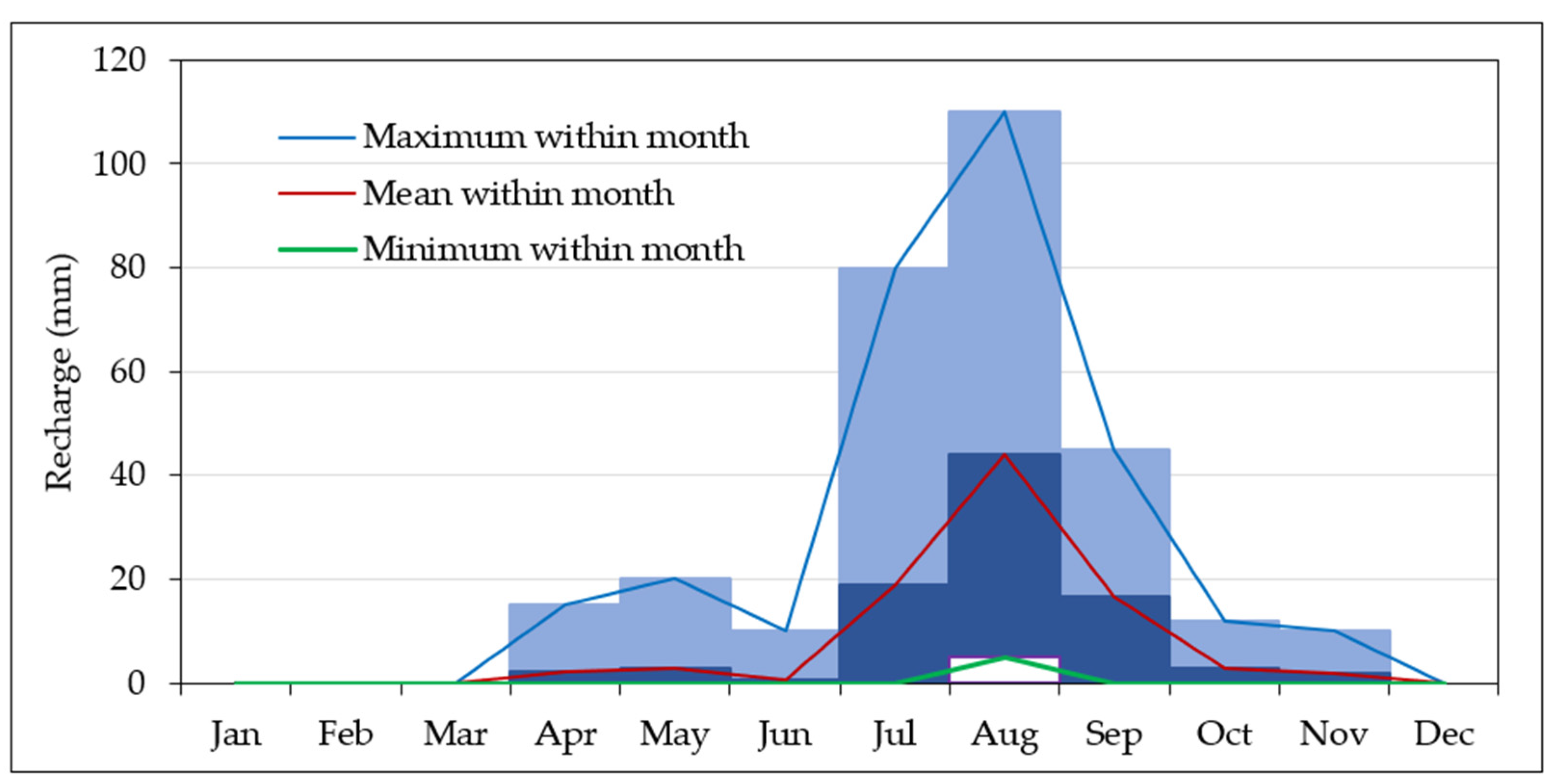
The long-term estimates of monthly recharge and runoff time series indicated that the water balance components follow the temporal pattern of rainfall amount. This implies that rainfall variability and the number of dry and wet episodes determine the rate and pattern of the water balance components. However, the relation of recharge to precipitation is not linearly related, and it is observed that it requires the exceedance of precipitation to produce substantial recharge. During dry months of zero or minimum observed precipitation, all precipitation is lost to evapotranspiration and soil-moisture replenishment. The simulated recharge showed zero values during the dry to low precipitation months. During months of high precipitation, for example, a small portion of precipitation is lost to evapotranspiration and soil-moisture replenishment, and the remaining contributes to recharge and runoff. That is why significant runoff peaks are always observed ahead of recharge. It is noticed from Figure 8 that the most notable peaks of runoff occur in July and August, whereas for recharge, the peaks start in July and end in September. In September, a more significant portion of the precipitation (24% of rainfall amount) contributes to recharge. This nonlinearity, in fact, reflects that changes in evapotranspiration and soil moisture are not proportional to changes in precipitation. In the mountains, a larger proportion of annual precipitation becomes runoff and recharge. However, in general, in the valley area, evapotranspiration and soil-moisture replenishment remove most incoming water, thus preventing conditions that lead to runoff and recharge.
The modeling result indicated that the valley floor and the adjacent mountain area receive different mean monthly recharges (Figure 9). The mean monthly recharge ranged from 0 mm (December to March) to 46 mm in August (accounting for 17% of rainfall amount). From December to March, there was low rainfall and the watershed was dry; therefore, the available rainfall first satisfies the moisture deficit in the catchment before contributing to recharge. Then, a small amount of recharge was observed in the month of April and the proportion of precipitation to contribute to recharge continued increasing until September where 11.64 mm (24% of rainfall amount) of recharge was observed. Similarly, the mean monthly runoff ranged from 0 mm in December–March to the 84 mm peak in August. The recharge and runoff minimum values were observed on the valley floor of the study area, with the maximum occurring in the mountainous part. A higher proportion of recharge (over 85% of the annual recharge) occurred in July, August, and September during periods of high rainfall. On the contrary, during the dry months, there was no recharge. This causes increased landscape stress or climatic water deficit, which, on the other hand, increases the reliance on withdrawing groundwater to meet water demands in the valley. The estimated hydrologic derivatives of this study result, the recharge and runoff quantities can be used to plan for water and land resource demands. Monthly groundwater withdrawals should consider the spatial and temporal recharge patterns.
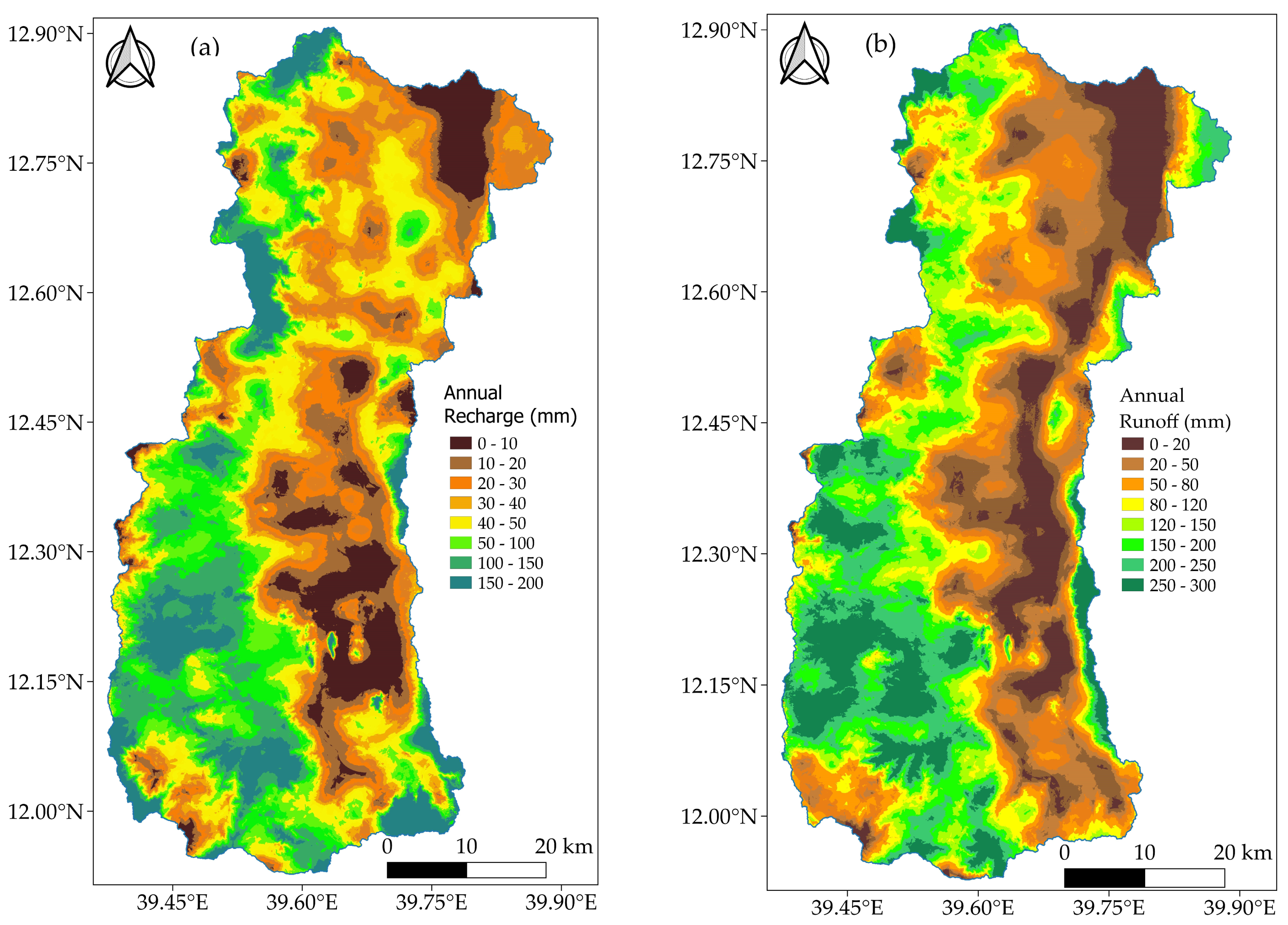
Recharge and runoff were also observed to spatially vary, where the maximum is estimated in the volcanic rocks of the mountains and the minimum on the valley floor of the alluvial deposits. Figure 10 shows the yearly average spatial variation in the estimated recharge and runoff for the groundwater basin and the surrounding mountain from 1991 to 2020. The average annual recharge varies from a minimum of 0 mm on the valley floor of the alluvial aquifer to a maximum of 200 mm in the high elevations of the volcanic mountains. Similarly, the average surface runoff varies from a minimum of 0 mm on the valley floor to a maximum of 300 mm in the mountains. The average amount for the study area is 73 mm for recharge and 169 mm for runoff. One third of the rainfall in the drainage basin becomes recharge and runoff, while the remaining two-thirds is lost through evapotranspiration. Despite the considerable percentage of rainfall amount being lost to evapotranspiration, more water is able to infiltrate into the soil and percolate to recharge the groundwater system in the wet months, particularly in August, which coincides with the month of the highest rainfall in the basin. The result indicates that the recharge represents a reasonable distribution of the hydrologic conditions throughout the study area, including precipitation timing and variation and varying bedrock types and soil depths.
The western part of the study area is topographically elevated and mountainous, with thin soils that cover the underlying, predominantly Ashange basalt. This mountainous part is thus topographically and geologically distinct from the adjacent lowland areas, which are relatively flat and underlain by thick unconsolidated sediments of alluvial basin-fill deposits that form highly productive aquifers (Figure 2). Higher elevations receive proportionately higher amounts of precipitation and experience lower air temperatures than the foothills and valley bottoms. This was confirmed as the BCM simulated recharge and runoff maps showed significantly higher values in the highlands (Figure 10a). The BCM generates recharge and runoff maps indicating the quantity and where in the watershed they are generated. Substantial recharge typically does not occur in the center of a structural basin without a perennial or intermittent streamflow therein. However, a significant component of recharge to basin aquifers occurs in coarse alluvium along the mountain front in semi-arid climates [25,71,72,73].
Precipitation is the most important variable contributing to the variation in recharge in this study. The amount of precipitation is the highest controlling factor for the spatial recharge estimation, which confirms the result from the findings of Kim and Jackson [74], who found that precipitation had the strongest effect. Nolan and Healy [75] also studied the factors influencing the spatial variation in recharge in the Eastern United States and confirmed that precipitation is the region’s most influencing factor for variation. Our study area is a semi-arid climate characterized by an extreme water deficit from evaporation exceeding precipitation. This illustrates the nonlinear relationship of precipitation to recharge in a semi-arid watershed. Describing the episodic nature of recharge as illustrated by [76], occurring when precipitation by far exceeds PET, the rainfall in previous months should first satisfy the moisture deficit in the catchment before contributing to recharge. The study in the semi-arid climate in Western Australia by Skrzypek and Siller [77] also confirms the same result, showing that recharge is episodical and occurs only after a considerable amount of precipitation, while all other precipitation events are quickly lost to evaporation [76].
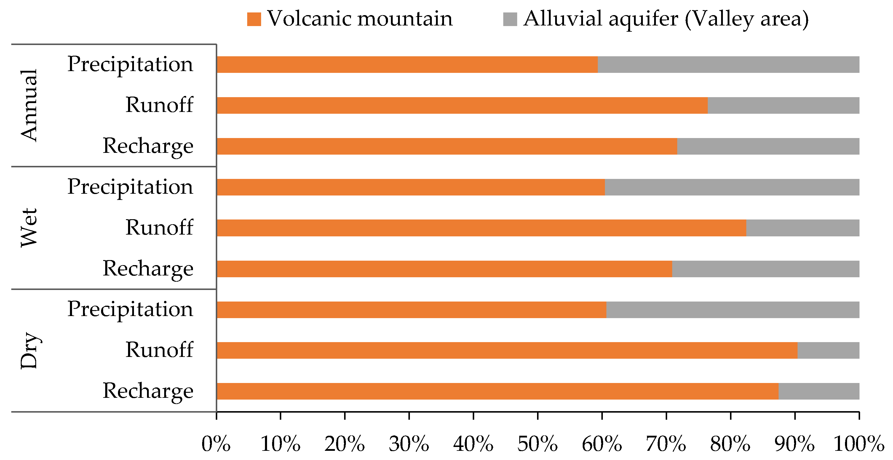
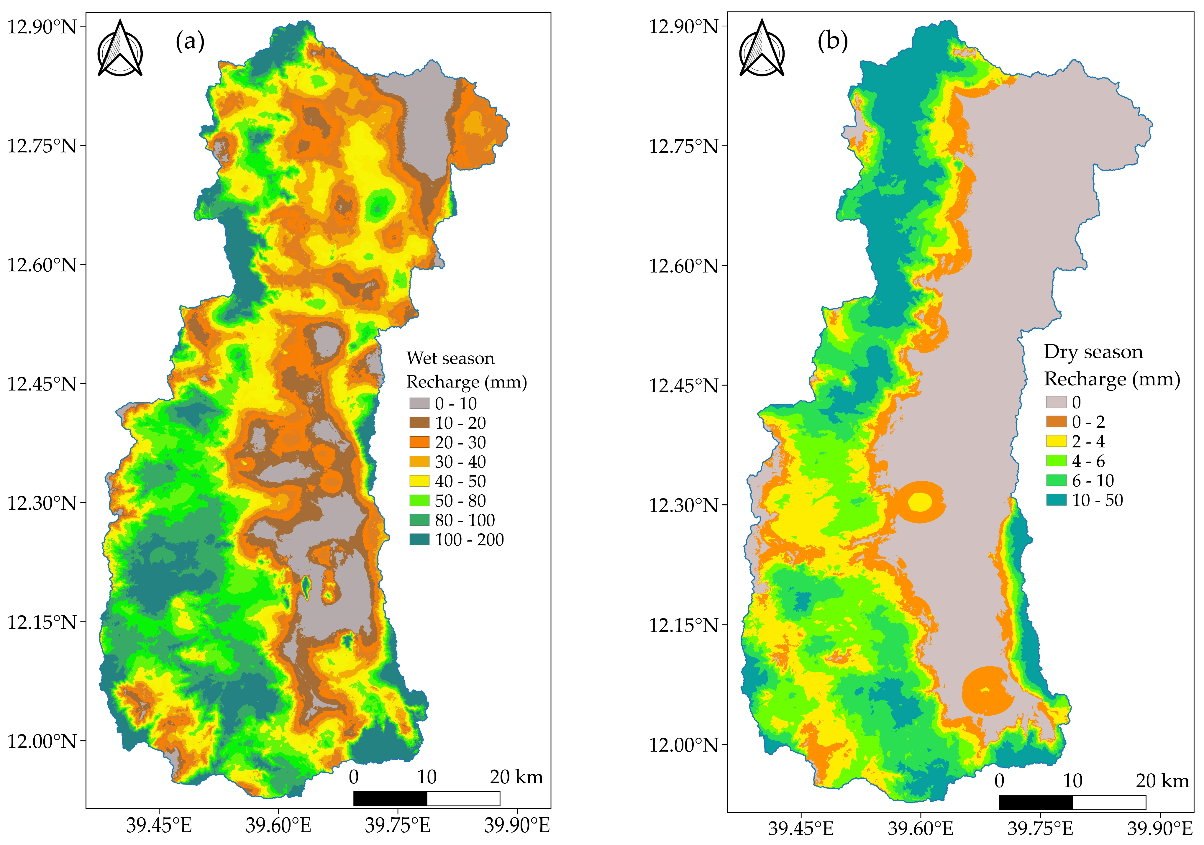
The long-term average results of BCM modeling for Raya and Kobo Valleys are summarized in Table 3. Over 81% of the total annual recharge in the drainage basin occurs in the wet season, while the remaining 19% occurs during the dry season. Dry season recharge spatially varies between 0 mm on the valley floor and 50 mm in the mountains, whereas most recharge occurs in the wet season, with a variation from 0 mm for 3% of the area on the valley floor to 200 mm for 2% of the area in the mountains (Figure 11 and Figure 12). The average annual runoff also shows a similar pattern to recharge, with 83% during the wet season and the remaining 17% contribution during dry seasons to the annual runoff. During the dry season, the runoff varies between 0 mm and 70 mm from the valley floor to the mountains, respectively, while an enormous runoff occurs during the summer rainy season between 0 mm for 3% of the area in the valley and 250 mm for 9% of the higher volcanic area. The dry season is characterized by high evapotranspiration and little surface runoff, often resulting in no recharge. In the wet season, the surface runoff increases, but evapotranspiration drops because of lower temperatures. Hence, more water is available for recharge.
Simulated recharge and runoff are also dependent on soil types. For the light soil types, loamy and sandy loam soil, recharge shows higher values, while for the heavier soils (silty clay and black cotton soil), recharge shows lower values. As a result, the western volcanic mountains have a relatively high recharge due to the high annual rainfall and loamy and sandy loam soil. On the contrary, in the lowland areas, in the eastern part of the study area, a relatively low recharge amount is calculated due to silty clay and black cotton soil in addition to the low rainfall and high evapotranspiration rate amount compared to the western highland areas. This has indicated that on the valley floor with thicker soil relative to the mountain part, a greater volume of water is needed than for the thin soil in the mountain part to exceed the soil-water storage capacity of the root zone. When the soil-water storage capacity is high, and the hydraulic conductivity of the soil is low, for example, for the silt clay, the drainage through the root zone occurs slowly, and evapotranspiration has more time to remove stored water between periods of precipitation and run-on from the gentle slopes on the valley floor. A high runoff of over 250 mm occurs on loam, sandy loam, and loamy sand soil types in high-slope areas in western volcanic mountains. In contrast, low runoff occurs in silty clay and black cotton soil in alluvial aquifers in the valley due to the gentle topography. The results shown demonstrate that most of the recharge occurs in the mountains part. This was an expected result because, as indicated above, the mountains typically have higher precipitation, lower air temperatures, and thinner soils relative to the valley floors.
Land use and land cover also influence the simulated recharge and runoff. For cultivation areas, there is an apparent influence of the seasons. It is assumed that the land in the dry season is almost bare, which results in increased surface runoff and higher actual evapotranspiration. The wet season is characterized by a higher annual rainfall, cooler air temperature, and reduced actual evapotranspiration, enabling higher recharge.
The average annual recharge estimated is 73 mm, accounting for 9% of the mean annual precipitation. The average yearly surface runoff estimated is 167 mm, accounting for 21% of the mean annual precipitation. This result is comparable to many studies that estimated recharge and runoff using the WetSpass model in Ethiopia with similar climatic conditions. For example, for Northern Ethiopia, ref. [78] estimated 7.9% of recharge and 13.7% of surface runoff of the mean annual precipitation, and for the southwestern escarpment of the main Ethiopian Rift, ref. [79] estimated 9.4% of recharge and 20% of surface runoff of the mean annual precipitation. In this regard, the current study’s findings confirm evidence from previous work conducted in volcanic aquifers with variable topography [80], where the spatial variation in recharge is influenced by topography, geomorphology, geology, and climatic setting, and higher recharges are observed in or adjacent to steep-sloping topographies, whereas valley bottoms experienced small recharges.
The spatially and temporally distributed estimates of recharge and runoff provided a means to investigate the fundamental concepts and evaluate mechanisms that control recharge in the study area. The effects of precipitation, soil properties including thickness, and hydraulic permeability of the underlying geologic materials were evaluated by using the BCM. As explained earlier, the study area is characterized by two geomorphic features—the surrounding mountains and the alluvial basin floor—which is the structural groundwater basin in the study area. The observed recharge in the mountain includes infiltration from precipitation and streams near mountain fronts and percolation through the mountain block, reaching the adjacent alluvial basin floor. Conceptually, this process is classified into two recharge processes. One is as a mountain-block recharge, where the water recharges directly into the bedrock and the groundwater inflows to a lowland aquifer from an adjacent mountain block. The other is as a mountain-front recharge, where a fault-controlled recharge occurs to the coarser sediments that are present along the basalt-alluvium contact, veneered by thin soils and that grade into the finer alluvium on the valley floor. Many studies have recognized the importance of mountain-front and mountain-block recharge as the main sources of water for arid and semi-arid regions [71,73].
4. Conclusions
In the ever-increasing water scarcity around the world, sustainable management of groundwater resources is of prime concern, in particular in arid and semi-arid regions. However, the data paucity in these regions and the limitations in available approaches are challenges in regard to precisely estimating groundwater recharge—pivotal for the sustainable use and development of groundwater. Therefore, the current study developed an approach for a reliable estimation of recharge by combining local and global datasets using a Basin Characterization Model (BCM). The execution of the two-step calibration method was adopted to reduce the uncertainty in the recharge estimate. This study was conducted in the Raya and Kobo Valley basins, a semi-arid area in Northern Ethiopia, covering 3506 km2. Climatic Research Unit monthly datasets (1991 to 2020) and WaPOR evapotranspiration data were used.
The model results show that the recharge and runoff are spatially and temporally variable. The average annual recharge ranged from 0 mm (3% of the area in the valley’s center) to about 200 mm (2% of the area in the adjacent western range). The average annual runoff ranged from 0 mm (3% of the area in the middle of the valley) to 300 mm (12% of the area at the highlands). Over 80% of the annual recharge and runoff occurs during the rainy season. The average annual recharge was estimated at 73 mm, about 9% of the mean annual precipitation, while the surface runoff was found at 167 mm constituting 21% of the mean annual precipitation.
The estimated monthly recharge and runoff time series (1991 to 2020) indicated that the water balance components follow the temporal pattern of precipitation amount. The quantified recharge in the alluvial deposits on the valley floor was found to be low because of the deep soil holding the water and the lowland areas receiving low amounts of precipitation. The valleys, which are relatively open and warmer, have a higher evapotranspiration, and the mountainous part experiences a lower evapotranspiration due to its high elevation and colder climate.
The capacity of watershed models such as the BCM to simulate at a finer spatial resolution (e.g., 10 m by 10 m) allows for overcoming data scarcity problems at smaller watershed levels. The recent improvements in water balance modeling enabling the refinement of water balance components contributed to an improvement in its precise estimation. Moreover, the water balance models were crucial in making data available in data-scarce regions that can be used as a boundary condition for the three-dimensional groundwater model to improve groundwater water modeling. Generally, in semi-arid regions suffering from data availability challenges, using water balance models by merging local and global data sources enables reliable estimation of the spatial and temporal distribution of hydrologic variables to assess water availability and develop management strategies for coping with the ever-increasing water demand. This could be further enhanced by coupling the BCM results as a boundary condition to a conjunctive use and landscape simulation model of the valley floor, such as MODFLOW-OWHM [31,32,35,36,81] for water resources management.
The improvement in the BCM focused on refining the actual evapotranspiration component, consequently enabling reliable recharge estimation. The improvement in this component was enabled by the availability of a national, gridded actual-evapotranspiration product from the WaPOR remotely sensed data. The main limitation of the model capabilities of the current version of the BCM is the reliance on a land use static property layer, which does not account for the temporal variation in the impact of land use land cover change on the water balance components. Hence, future predictions should take this limitation into consideration for improvement.
The results of the current study are crucial for water managers and stakeholders to develop plans for sustainable groundwater resource management. The results from this study can also be used to provide inputs to a three-dimensional groundwater model to analyze the available resources against the growing water demands for future groundwater availability and management. In general, the water balance model BCM, climate datasets, and remote sensing data are viable options for the reliable estimation of the recharge and runoff in data-scarce developing regions of the world for sustainable management of groundwater resources.
Author Contributions
Conceptualization, S.S.M., S.E.B., A.K.M. and M.D.; methodology, S.S.M.; software, S.S.M., L.F., A.F. and S.E.B.; validation, S.S.M., S.E.B. and M.D.; formal analysis, S.S.M.; resources, S.S.M., L.F. and A.F.; data curation, S.S.M.; writing—original draft preparation, S.S.M.; writing—review and editing, S.S.M., L.F., A.F., S.E.B., A.K.M. and M.D.; supervision, S.E.B., A.K.M. and M.D. All authors have read and agreed to the published version of the manuscript.
Funding
This article was accomplished in the framework of the Home-Grown Scholarship Program funded by the governments of Ethiopia and the German Academic Exchange Service (DAAD). The project was implemented by Arba Minch University Water Research Center, Ethiopia (GOV/AMU/TH01/AWTI/WRRC/092014), in cooperation with the Chair of Hydrology and River Basin Management at the Technical University of Munich, Germany. In addition, this work was supported by the German Research Foundation (DFG) and the Technical University of Munich in the framework of the Open Access Publishing Program.
Institutional Review Board Statement
Not applicable.
Informed Consent Statement
Not applicable.
Data Availability Statement
Data are contained within the article.
Acknowledgments
The authors are very grateful to the Chair of Hydrology and River Basin Management at the Technical University of Munich (TUM) and its Graduate School (TUM-GS) and Arba Minch University, Ethiopia, for the institutional services and facilities necessary to perform this study. The authors also thank the Office of Ethiopian Construction Design and Supervision Works Corporation (ECDSWC); the Ethiopian Ministry of Water, Irrigation and Energy (MWIE); and the Ethiopian National Meteorological Agency (ENMA) for providing the necessary geology and hydro meteorological data. Additionally, they acknowledge Randy Hanson, President and Hydrologist at One-Water Hydrologic, and Zerihun Anbessa for constructive comments throughout the research work, as well as William C. Steinkampf, Director of Science Coordination at Earth Knowledge Inc., for the review of the journal article. They would also like to thank Nicole Parker for technical rhetoric comments and editorial comments.
Conflicts of Interest
Authors Lorraine Flint and Alan Flint were employed by the company Earth Knowledge Inc. The remaining authors declare that the research was conducted in the absence of any commercial or financial relationships that could be construed as a potential conflict of interest.
Disclaimer
Any use of trade, firm, or product names is for descriptive purposes only and does not imply endorsement by the U.S. Government. This journal article has been peer reviewed and approved for publication consistent with USGS Fundamental Science Practices (https://pubs.usgs.gov/circ/1367/).
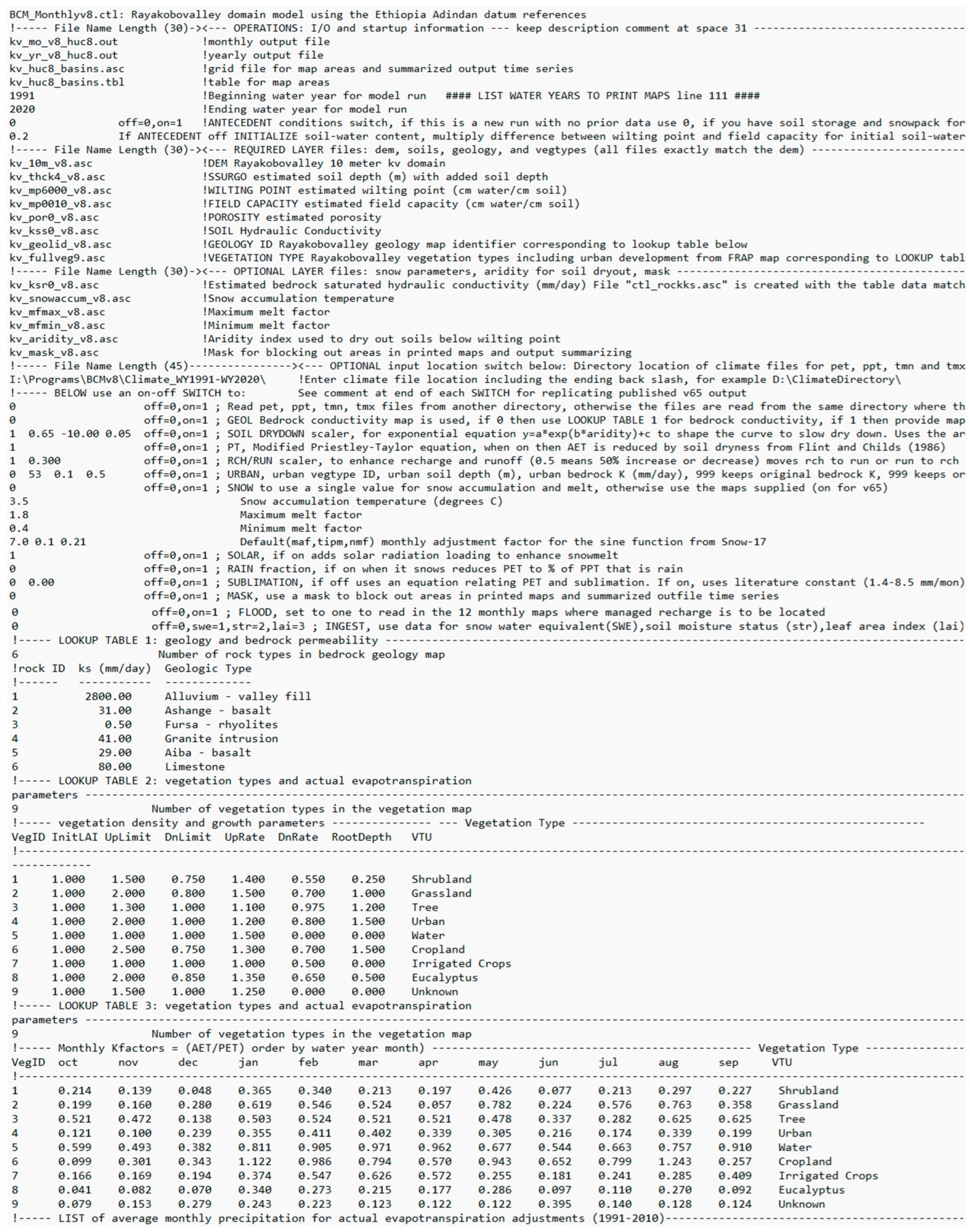
Appendix A
Figure A1.
Control file for BCM.

Appendix B

Table A1.
Calibrated values of the vegetation density and growth parameters (source of initial estimate: [13]).
Table A1.
Calibrated values of the vegetation density and growth parameters (source of initial estimate: [13]).
| Vegetation Type | Calibrated Value | |||||
|---|---|---|---|---|---|---|
| InitLAI | UpLimit | DnLimit | UpRate | DnRate | RootDepth | |
| Initial value | 0 to 1 | 1 to 3.5 | 0.5 to 1 | 1 to 2.5 | 0.5 to 1 | 0 to 2.5 |
| Shrubland | 1.00 | 1.50 | 0.75 | 1.40 | 0.55 | 0.25 |
| Grassland | 1.00 | 2.00 | 0.80 | 1.50 | 0.70 | 1.00 |
| Tree | 1.00 | 1.30 | 1.00 | 1.10 | 0.98 | 1.20 |
| Urban | 1.00 | 2.00 | 1.00 | 1.20 | 0.80 | 1.50 |
| Water | 1.00 | 1.00 | 1.00 | 1.50 | 0.00 | 0.00 |
| Cropland | 1.00 | 2.50 | 0.75 | 1.30 | 0.70 | 1.50 |
| Irrigated crops | 1.00 | 1.00 | 1.00 | 1.00 | 0.50 | 0.00 |
| Eucalyptus | 1.00 | 2.00 | 0.85 | 1.35 | 0.65 | 0.50 |
Appendix C
Table A2.
Calibrated bedrock conductivities. Results of final calibrated bedrock conductivities (source of initial estimate: Ethiopian Construction Design & Supervision Works Corporation (CDSWC) office; [13]).
Table A2.
Calibrated bedrock conductivities. Results of final calibrated bedrock conductivities (source of initial estimate: Ethiopian Construction Design & Supervision Works Corporation (CDSWC) office; [13]).
| Geologic Type | Bedrock Conductivity, Ks (m/day) | |
|---|---|---|
| Initial Value | Calibrated Value | |
| Alluvium | 6.65 | 2.8 |
| Ashange basalt | 0.032 | 0.031 |
| Fursa rhyolite | 0.0005 | 0.0005 |
| Granite intrusion | 0.0015 | 0.041 |
| Aiba basalt | 0.003 | 0.029 |
| Limestone | 0.1 | 0.08 |
References
- Adelana, M.; Macdonald, A. Groundwater Research Issues in Africa; CRC Press: Boca Raton, FL, USA, 2008. [Google Scholar]
- Gaye, C.B.; Tindimugaya, C. Review: Challenges and opportunities for sustainable groundwater management in Africa. Hydrogeol. J. 2018, 27, 1099–1110. [Google Scholar] [CrossRef]
- Scanlon, B.R.; Keese, K.E.; Flint, A.L.; Flint, L.E.; Gaye, C.B.; Edmunds, W.M.; Simmers, I. Global synthesis of groundwater recharge in semiarid and arid regions. Hydrol. Process. 2006, 20, 3335–3370. [Google Scholar] [CrossRef]
- Ahmed, A.K.A.; El-Rawy, M.; Ibraheem, A.M.; Al-Arifi, N.; Abd-Ellah, M.K. Forecasting of Groundwater Quality by Using Deep Learning Time Series Techniques in an Arid Region. Sustainability 2023, 15, 6529. [Google Scholar] [CrossRef]
- Uugulu, S.; Wanke, H. Estimation of groundwater recharge in savannah aquifers along a precipitation gradient using chloride mass balance method and environmental isotopes Namibia. Phys. Chem. Earth 2020, 116, 1028844. [Google Scholar] [CrossRef]
- Healy, R.W.; Cook, P.G. Using groundwater levels to estimate recharge. Hydrogeol. J. 2002, 10, 91–109. [Google Scholar] [CrossRef]
- Messerschmid, C.; Aliewi, A. Spatial distribution of groundwater recharge, based on regionalised soil moisture models in Wadi Natuf karst aquifers, Palestine. Hydrol. Earth Syst. Sci. 2022, 26, 1043–1061. [Google Scholar] [CrossRef]
- Dubois, E.; Larocque, M.; Gagné, S.; Meyzonnat, G. Simulation of long-term spatiotemporal variations in regional-scale groundwater recharge: Contributions of a water budget approach in cold and humid climates. Hydrol. Earth Syst. Sci. 2021, 25, 6567–6589. [Google Scholar] [CrossRef]
- Demissie, E.S.; Gashaw, D.Y.; Altaye, A.A.; Demissie, S.S.; Ayele, G.T. Groundwater Recharge Estimation in Upper Gelana Watershed, South-Western Main Ethiopian Rift Valley. Sustainability 2023, 15, 1763. [Google Scholar] [CrossRef]
- Kafando, M.B.; Koïta, M.; Zouré, C.O.; Yonaba, R.; Niang, D. Quantification of Soil Deep Drainage and Aquifer Recharge Dynamics according to Land Use and Land Cover in the Basement Zone of Burkina Faso in West Africa. Sustainability 2022, 14, 14687. [Google Scholar] [CrossRef]
- Hornero, J.; Manzano, M.; Ortega, L.; Custodio, E. Integrating soil water and tracer balances, numerical modelling and GIS tools to estimate regional ground-water recharge: Application to the Alcadozo Aquifer System (SE Spain). Sci. Total Environ. 2016, 568, 415–432. [Google Scholar] [CrossRef]
- Stern, M.A.; Flint, L.E.; Flint, A.L.; Christensen, A.H. A Basin-Scale Approach to Estimating Recharge in the Desert: Anza-Cahuilla Groundwater Basin, CA. J. Am. Water Resour. Assoc. 2021, 57, 990–1003. [Google Scholar] [CrossRef]
- Flint, L.E.; Flint, A.L.; Stern, M.A. The Basin Characterization Model—A Regional Water Balance Software Package, in Techniques and Methods; U.S. Geological Survey: Reston, VA, USA, 2021; p. 85.
- Dripps, W.R.; Bradbury, K.R. A simple daily soil–water balance model for estimating the spatial and temporal distribution of groundwater recharge in temperate humid areas. Hydrogeol. J. 2007, 15, 433–444. [Google Scholar] [CrossRef]
- Healy, R.W. Estimating Groundwater Recharge; Cambridge University Press: Cambridge, UK, 2010. [Google Scholar]
- Jiménez-Martínez, J.; Longuevergne, L.; Le Borgne, T.; Davy, P.; Russian, A.; Bour, O. Temporal and spatial scaling of hydraulic response to recharge in fractured aquifers: Insights from a frequency domain analysis. Water Resour. Res. 2013, 49, 3007–3023. [Google Scholar] [CrossRef]
- Scanlon, B.R.; Cook, P.G. Theme issue on groundwater recharge. Hydrogeol. J. 2002, 10, 3–4. [Google Scholar] [CrossRef]
- Scanlon, B.R.; Healy, R.W.; Cook, P.G. Choosing appropriate techniques for quantifying groundwater recharge. Hydrogeol. J. 2002, 10, 18–39. [Google Scholar] [CrossRef]
- Xie, Y.; Cook, P.G.; Simmons, C.T.; Partington, D.; Crosbie, R.; Batelaan, O. Uncertainty of groundwater recharge estimated from a water and energy balance model. J. Hydrol. 2018, 561, 1081–1093. [Google Scholar] [CrossRef]
- Allison, G.B.; Gee, G.W.; Tyler, S.W. Vadose-Zone Techniques for Estimating Groundwater Recharge in Arid and Semiarid Regions. Soil Sci. Soc. Am. J. 1994, 58, 6–14. [Google Scholar] [CrossRef]
- Flint, L.E.; Flint, A.L.; Thorne, J.H.; Boynton, R. Fine-scale hydrologic modeling for regional landscape applications: The California Basin Characterization Model development and performance. Ecol. Process. 2013, 2, 25. [Google Scholar] [CrossRef]
- Hutchinson, D.G.; Moore, R.D. Throughflow variability on a forested hillslope underlain by compacted glacial till. Hydrol. Process. 2000, 14, 1751–1766. [Google Scholar] [CrossRef]
- Hopp, L.; McDonnell, J. Connectivity at the hillslope scale: Identifying interactions between storm size, bedrock permeability, slope angle and soil depth. J. Hydrol. 2009, 376, 378–391. [Google Scholar] [CrossRef]
- Flint, L.E.; Flint, A.L. Regional Analysis of Ground-Water Recharge, in Professional Paper; Stonestrom, D.A., Ed.; U.S. Geological Survey: Reston, VA, USA, 2007; pp. 29–60.
- Flint, A.L.; Flint, L.E.; Hevesi, J.A.; Blainey, J.B. Fundamental Concepts of Recharge in the Desert Southwest: A Regional Modeling Perspective. In Ground-Water Recharge in a Desert Environment: The Southwestern United States; American Geophysical Union: Washington, DC, USA, 2004; pp. 159–184. [Google Scholar]
- Flint, L.E.; Flint, A.L. Downscaling future climate scenarios to fine scales for hydrologic and ecological modeling and analysis. Ecol. Process. 2012, 1, 2. [Google Scholar] [CrossRef]
- Flint, L.E.; Flint, A.L. Simulation of climate change in San Francisco Bay Basins, California: Case Studies in the Russian River Valley and Santa Cruz Mountains, in Scientific Investigations Report; U.S. Geological Survey: Reston, VA, USA, 2012; p. 61.
- Flint, L.E.; Flint, A.L.; Curtis, J.A.; Delaney, C.; Mendoza, J. Provisional Simulated Unimpaired Mean Daily Streamflow in the Russian River and Upper Eel River Basins, California, Under Historical and Projected Future Climates; U.S. Geological Survey: Reston, VA, USA, 2015.
- Thorne, J.H.; Boynton, R.M.; Flint, L.E.; Flint, A.L. The magnitude and spatial patterns of historical and future hydrologic change in California’s watersheds. Ecosphere 2015, 6, art24. [Google Scholar] [CrossRef]
- Micheli, E.; Dwight Center for Conservation Science at Pepperwood Preserve; Flint, L.; Flint, A.; Weiss, S.; Kennedy, M.; Survey, U.G.; Observation, C.C.F.E. Downscaling Future Climate Projections to the Watershed Scale: A North San Francisco Bay Case Study. San Fr. Estuary Watershed Sci. 2012, 10. [Google Scholar] [CrossRef]
- Hanson, R.T.; Flint, L.E.; Faunt, C.C.; Gibbs, D.R.; Schmid, W. Hydrologic models and analysis of water availability in Cuyama Valley, California. In Scientific Investigations Report; U.S. Geological Survey: Reston, VA, USA, 2014; p. 166. [Google Scholar]
- Faunt, C.C.; Stamos, C.L.; Flint, L.E.; Wright, M.T.; Burgess, M.K.; Sneed, M.; Brandt, J.; Martin, P.; Coes, A.L. Hydrogeology, Hydrologic Effects of Development, and Simulation of Groundwater Flow in the Borrego Valley, San Diego County, California. In Scientific Investigations Report; U.S. Geological Survey: Reston, VA, USA, 2015. [Google Scholar]
- Phillips, S.P.; Rewis, D.L.; Traum, J.A. Hydrologic Model of the Modesto Region, California, 1960–2004. In Scientific Investigations Report; U.S. Geological Survey: Reston, VA, USA, 2015; p. 84. [Google Scholar]
- Siade, A.; Nishikawa, T.; Martin, P. Natural recharge estimation and uncertainty analysis of an adjudicated groundwater basin using a regional-scale flow and subsidence model (Antelope Valley, California, USA). Hydrogeol. J. 2015, 23, 1267–1291. [Google Scholar] [CrossRef]
- Boyce, S.E.; Hanson, R.T.; Ferguson, I.; Schmid, W.; Henson, W.R.; Reimann, T.; Mehl, S.W.; Earll, M.M. One-Water Hydrologic Flow Model: A Modflow Based Conjunctive-Use Simulation Software. In Techniques and Methods; U.S. Geological Survey: Reston, VA, USA, 2020; p. 435. [Google Scholar]
- Boyce, S.E. Modflow One-Water Hydrologic Flow Model (MF-OWHM) Conjunctive Use and Integrated Hydrologic Flow Modeling Software, version 2.3.0.; U.S. Geological Survey: Reston, VA, USA, 2023.
- Byrd, K.B.; Flint, L.E.; Alvarez, P.; Casey, C.F.; Sleeter, B.M.; Soulard, C.E.; Flint, A.L.; Sohl, T.L. Integrated climate and land use change scenarios for California rangeland ecosystem services: Wildlife habitat, soil carbon, and water supply. Landsc. Ecol. 2015, 30, 729–750. [Google Scholar] [CrossRef]
- Stern, M.A.; Flint, L.E.; Flint, A.L. Characterization of hydrology and sediment transport following drought and wildfire in Cache Creek, California. In Proceedings of the SEDHYD, Federal Interagency Sedimentation Conference (FISC) and Federal Interagency Hydrologic Modeling Conference (FIHMC), Reno, NV, USA, 24–28 June 2019. [Google Scholar]
- Flint, L.E.; Flint, A.L.; Stern, M.A.; Mayer, A.; Silver, W.; Franco, F.; Byrd, K.; Sleeter, B.; Alvarez, P.; Creque, J.; et al. Increasing Soil Organic Carbon to Mitigate Greenhouse Gases and Increase Climate Resiliency for California; Cailfornia Natural Resorces Agency: Sacramento, CA, USA, 2018.
- Muñoz-Rojas, M.; Erickson, T.E.; Dixon, K.W.; Merritt, D.J. Soil quality indicators to assess functionality of restored soils in degraded semiarid ecosystems. Restor. Ecol. 2016, 24, S43–S52. [Google Scholar] [CrossRef]
- Weiss, S.; Flint, A.; Flint, L.; Hamilton, H.; Fernandez, M.; Micheli, L. High Resolution Climate-Hydrology Scenarios for San Francisco ’s Bay Area; Dwight Center for Conservation Science at Pepperwood: Santa Rosa, CA, USA, 2013; p. 60. [Google Scholar]
- Hannah, L.; Steele, M.; Fung, E.; Imbach, P.; Flint, L.; Flint, A. Climate change influences on pollinator, forest, and farm interactions across a climate gradient. Clim. Chang. 2016, 141, 63–75. [Google Scholar] [CrossRef]
- Li, W.; An, M.; Wu, H.; An, H.; Huang, J.; Khanal, R. The local coupling and telecoupling of urbanization and ecological environment quality based on multisource remote sensing data. J. Environ. Manag. 2023, 327, 116921. [Google Scholar] [CrossRef]
- Vergara, H.; Hong, Y.; Gourley, J.J.; Anagnostou, E.N.; Maggioni, V.; Stampoulis, D.; Kirstetter, P.-E. Effects of Resolution of Satellite-Based Rainfall Estimates on Hydrologic Modeling Skill at Different Scales. J. Hydrometeorol. 2014, 15, 593–613. [Google Scholar] [CrossRef]
- Gourley, J.J.; Vieux, B.E. A Method for Evaluating the Accuracy of Quantitative Precipitation Estimates from a Hydrologic Modeling Perspective. J. Hydrometeorol. 2005, 6, 115–133. [Google Scholar] [CrossRef]
- Lewis, F.; Walker, G. Assessing the potential for episodic recharge in south-western Australia using rainfall data. Hydro. Geol. J. 2002, 10, 229–237. [Google Scholar]
- Ackerly, D.D.; Loarie, S.R.; Cornwell, W.K.; Weiss, S.B.; Hamilton, H.; Branciforte, R.; Kraft, N.J.B. The geography of climate change: Implications for conservation biogeography. Divers. Distrib. 2010, 16, 476–487. [Google Scholar] [CrossRef]
- Franklin, J.; Davis, F.W.; Ikegami, M.; Syphard, A.D.; Flint, L.E.; Flint, A.L.; Hannah, L. Modeling plant species distributions under future climates: How fine scale do climate projections need to be? Glob. Chang. Biol. 2013, 19, 473–483. [Google Scholar] [CrossRef]
- Tafesse, N.; Nedaw, D.; Woldearegay, K.; Gebreyohannes, T.; Steenbergen, F.V. Groundwater management for irrigation in the raya and kobo valleys, Northern Ethiopia. Int. J. Earth Sci. Eng. 2015, 8, 1104–1114. [Google Scholar]
- Corti, G.; Bastow, I.D.; Keir, D.; Pagli, C.; Baker, E. Rift-Related Morphology of the Afar Depression. In Landscapes and Landforms of Ethiopia. World Geomorphological Landscapes; Billi, P., Ed.; Springer: Dordrecht, The Netherlands, 2015; pp. 251–274. [Google Scholar] [CrossRef]
- Zwaan, F.; Corti, G.; Keir, D.; Sani, F. A review of tectonic models for the rifted margin of Afar: Implications for continental break-up and passive margin formation. J. Afr. Earth Sci. 2019, 164, 103649. [Google Scholar] [CrossRef]
- Harris, I.; Osborn, T.J.; Jones, P.; Lister, D. Version 4 of the CRU TS monthly high-resolution gridded multivariate climate dataset. Sci. Data 2020, 7, 1–18. [Google Scholar] [CrossRef]
- Renard, D.; Tilman, D. National food production stabilized by crop diversity. Nature 2019, 571, 257–260. [Google Scholar] [CrossRef]
- Nalder, I.A.; Wein, R.W. Spatial interpolation of climatic Normals: Test of a new method in the Canadian boreal forest. Agric. For. Meteorol. 1998, 92, 211–225. [Google Scholar] [CrossRef]
- Bouwer, L.M.; Aerts, J.C.J.H.; Coterlet, G.V.D.; Giesen, N.V.D.; Gieske, A.; Mannaerts, C. Evaluating Downscaling Methods for Preparing Global Circulation Model (GCM) Data for Hydrological Impact Modelling. In Climate Change in Contrasting River Basins Adaptation Strategies for Water, Food and Environment; CABI Publishing: Wallingford, UK, 2004; pp. 25–47. [Google Scholar]
- Thorne, J.H.; Zboynton, R.; Flint, L.; Flint, A.; Lee, T. Development and Application of Downscaled Hydroclimatic Predictor Variables for Use in Climate Vulnera-Bility and Assessment Studies; University of California: Davis, CA, USA, 2012. [Google Scholar]
- Flint, A.L.; Childs, S.W. Use of the Priestley-Taylor evaporation equation for soil water limited conditions in a small forest clearcut. Agric. For. Meteorol. 1991, 56, 247–260. [Google Scholar] [CrossRef]
- Blatchford, M.L.; Mannaerts, C.M.; Njuki, S.M.; Nouri, H.; Zeng, Y.; Pelgrum, H.; Wonink, S.; Karimi, P. Evaluation of WaPOR V2 evapotranspiration products across Africa. Hydrol. Process. 2020, 34, 3200–3221. [Google Scholar] [CrossRef]
- Dile, Y.T.; Ayana, E.K.; Worqlul, A.W.; Xie, H.; Srinivasan, R.; Lefore, N.; You, L.; Clarke, N. Evaluating satellite-based evapotranspiration estimates for hydrological applications in data-scarce regions: A case in Ethiopia. Sci. Total. Environ. 2020, 743, 140702. [Google Scholar] [CrossRef]
- Gebremedhin, M.A.; Lubczynski, M.W.; Maathuis, B.H.; Teka, D. Deriving potential evapotranspiration from satellite-based reference evapotranspiration, Upper Tekeze Basin, Northern Ethiopia. J. Hydrol. Reg. Stud. 2022, 41, 101059. [Google Scholar] [CrossRef]
- Abate, B.Z.; Assefa, T.T.; Tigabu, T.B.; Abebe, W.B.; He, L. Hydrological Modeling of the Kobo-Golina River in the Data-Scarce Upper Danakil Basin, Ethiopia. Sustainability 2023, 15, 3337. [Google Scholar] [CrossRef]
- Wang, Y.; Zhang, S.; Chang, X. Evapotranspiration Estimation Based on Remote Sensing and the SEBAL Model in the Bosten Lake Basin of China. Sustainability 2020, 12, 7293. [Google Scholar] [CrossRef]
- Waqas, M.M.; Waseem, M.; Ali, S.; Leta, M.K.; Shah, A.N.; Awan, U.K.; Shah, S.H.H.; Yang, T.; Ullah, S. Evaluating the Spatio-Temporal Distribution of Irrigation Water Components for Water Resources Management Using Geo-Informatics Approach. Sustainability 2021, 13, 8607. [Google Scholar] [CrossRef]
- Weerasinghe, I.; Bastiaanssen, W.; Mul, M.; Jia, L.; Van Griensven, A. Can we trust remote sensing ET products over Africa? Hydrol. Earth Syst. Sci. Discuss. 2019, 24, 1565–1586. [Google Scholar] [CrossRef]
- Chukalla, A.D.; Mul, M.L.; van der Zaag, P.; van Halsema, G.; Mubaya, E.; Muchanga, E.; Besten, N.D.; Karimi, P. A framework for irrigation performance assessment using WaPOR data: The case of a sugarcane estate in Mozambique. Hydrol. Earth Syst. Sci. 2022, 26, 2759–2778. [Google Scholar] [CrossRef]
- QGIS Development Team. QGIS Geographic Information System; Open Source Geospatial Foundation: Beaverton, OR, USA, 2009. [Google Scholar]
- Nash, J.E.; Sutcliffe, J.V. River flow forecasting through conceptual models part I—A discussion of principles. J. Hydrol. 1970, 10, 282–290. [Google Scholar] [CrossRef]
- Moriasi, D.N.; Arnold, J.G.; van Liew, M.W.; Bingner, R.L.; Harmel, R.D.; Veith, T.L. Model evaluation guidelines for systematic quantification of accuracy in watershed simulations. Trans. ASABE 2007, 50, 885–900. [Google Scholar] [CrossRef]
- Legates, D.; McCabe, G. Evaluating the Use Of “Goodness-of-Fit” Measures in Hydrologic and Hydroclimatic Model Validation. Water Resour. Res. 1999, 35, 233–241. [Google Scholar] [CrossRef]
- Gupta, H.V.; Sorooshian, S.; Yapo, P.O. Status of Automatic Calibration for Hydrologic Models: Comparison with Multilevel Expert Calibration. J. Hydrol. Eng. 1999, 4, 135–143. [Google Scholar] [CrossRef]
- Markovich, K.H.; Manning, A.H.; Condon, L.E.; McIntosh, J.C. Mountain-Block Recharge: A Review of Current Understanding. Water Resour. Res. 2019, 55, 8278–8304. [Google Scholar] [CrossRef]
- Wilson, J.L.; Guan, H. Mountain-Block Hydrology and Mountain-Front Recharge. In Groundwater Recharge in a Desert Environment: The Southwestern United States; American Geophysical Union: Washington, DC, USA, 2004; pp. 113–137. [Google Scholar]
- Dar, T.; Rai, N.; Kumar, S. Distinguishing Mountain Front and Mountain Block Recharge in an Intermontane Basin of the Himalayan Region. Groundwater 2022, 60, 488–495. [Google Scholar] [CrossRef]
- Kim, J.H.; Jackson, R.B. A Global Analysis of Groundwater Recharge for Vegetation, Climate, and Soils. Vadose Zone J. 2012, 11, 0021RA. [Google Scholar] [CrossRef]
- Nolan, B.T.; Healy, R.W.; Taber, P.E.; Perkins, K.; Hitt, K.J.; Wolock, D.M. Factors influencing ground-water recharge in the eastern United States. J. Hydrol. 2007, 332, 187–205. [Google Scholar] [CrossRef]
- Flint, L.E.; Flint, A.L.; Stolp, B.J.; Danskin, W.R. A basin-scale approach for assessing water resources in a semiarid environment: San Diego region, California and Mexico. Hydrol. Earth Syst. Sci. 2012, 16, 3817–3833. [Google Scholar] [CrossRef]
- Skrzypek, G.; Siller, A.; McCallum, J.L.; Dogramaci, S. Groundwater recharge through internally drained basins in a semiarid climate, Western Australia. J. Hydrol. Reg. Stud. 2023, 47, 101388. [Google Scholar] [CrossRef]
- Gebru, T.A.; Tesfahunegn, G.B. GIS based water balance components estimation in northern Ethiopia catchment. Soil Tillage Res. 2019, 197, 104514. [Google Scholar] [CrossRef]
- Dereje, B.; Nedaw, D. Groundwater Recharge Estimation Using WetSpass Modeling in Upper Bilate Catchment, Southern Ethiopia. Momona Ethiop. J. Sci. 2019, 11, 37–51. [Google Scholar] [CrossRef]
- Yenehun, A.; Dessie, M.; Nigate, F.; Belay, A.S.; Azeze, M.; Van Camp, M.; Taye, D.F.; Kidane, D.; Adgo, E.; Nyssen, J.; et al. Spatial and temporal simulation of groundwater recharge and cross-validation with point estimations in volcanic aquifers with variable topography. J. Hydrol. Reg. Stud. 2022, 42, 101142. [Google Scholar] [CrossRef]
- Hanson, R.T.; Ritchie, A.B.; Boyce, S.E.; Ferguson, I.; Galanter, A.E.; Flint, L.E.; Henson, W.R. Rio Grande Transboundary Integrated Hydrologic Model and Water-Availability Analysis, New Mexico and Texas, United States, and Northern Chihuahua, Mexico, in Scientific Investigations Report; U.S. Geological Survey: Reston, VA, USA, 2020; p. 186.
Figure 1.
Raya and Kobo Valley drainage basins in the Ethiopian Main Rift, Great East African Rift Valley System.
Figure 1.
Raya and Kobo Valley drainage basins in the Ethiopian Main Rift, Great East African Rift Valley System.

Figure 2.
Raya and Kobo Valley’s geologic map with geologic bedrock conductivity (Ks).

Figure 3.
Raya and Kobo Valleys’ drainage basin: (a) soil map and (b) a land-use-type map (2020).

Figure 4.
Monthly actual evapotranspiration (AET) variation in Raya and Kobo Valleys. High and low ranges refer to the maximum and minimum actual evapotranspiration observed in a month in the study area, respectively.
Figure 4.
Monthly actual evapotranspiration (AET) variation in Raya and Kobo Valleys. High and low ranges refer to the maximum and minimum actual evapotranspiration observed in a month in the study area, respectively.

Figure 5.
Basin Characterization Model structure: water balance components, model input, process, and outputs (modified after [13]).
Figure 5.
Basin Characterization Model structure: water balance components, model input, process, and outputs (modified after [13]).

Figure 6.
Monthly AET comparison for remote sensing and BCM simulated for Raya and Kobo Valley with (a) no growth parameter adjustment and (b) growth parameters adjusted for annual precipitation variability.
Figure 6.
Monthly AET comparison for remote sensing and BCM simulated for Raya and Kobo Valley with (a) no growth parameter adjustment and (b) growth parameters adjusted for annual precipitation variability.

Figure 7.
Calibration and validation time series for comparison of the measured discharge and the discharge calculated with the BCM in the catchment area of the Golina discharge measuring station.
Figure 7.
Calibration and validation time series for comparison of the measured discharge and the discharge calculated with the BCM in the catchment area of the Golina discharge measuring station.

Figure 8.
Raya and Kobo Valleys simulated monthly recharge and runoff for water years 1991–2020.

Figure 9.
Raya and Kobo Valleys’ monthly maximum, minimum, and mean values of recharge during water years 1991–2020.
Figure 9.
Raya and Kobo Valleys’ monthly maximum, minimum, and mean values of recharge during water years 1991–2020.

Figure 10.
Raya and Kobo Valleys’ BCM mean annual for water years 1991–2020: (a) recharge and (b) runoff.
Figure 10.
Raya and Kobo Valleys’ BCM mean annual for water years 1991–2020: (a) recharge and (b) runoff.

Figure 11.
Percentage of annual and seasonal precipitation, recharge, and runoff occurrence in the volcanic mountain and the alluvial aquifer—the groundwater basin.
Figure 11.
Percentage of annual and seasonal precipitation, recharge, and runoff occurrence in the volcanic mountain and the alluvial aquifer—the groundwater basin.

Figure 12.
Maps of mean seasonal recharge for Raya and Kobo Valleys’ study area for water years 1991–2020 during (a) the wet season and (b) the dry season.
Figure 12.
Maps of mean seasonal recharge for Raya and Kobo Valleys’ study area for water years 1991–2020 during (a) the wet season and (b) the dry season.

Table 1.
Input data and output hydrologic variables for the Basin Characterization Model (BCM).
| Variable | Source | Type | Description |
|---|---|---|---|
| Climate datasets (maximum and minimum air temperature and precipitation (PCP)) | Climatic Research Unit transient monthly dataset | Model input | Maximum and minimum monthly air temperature (°C) and total monthly precipitation (mm) |
| Potential evapotranspiration (PET) | Modeled (pre-processed) | Model input | Total amount of water that can evaporate from ground surface and transpire from plant bodies (mm) |
| Digital elevation model (DEM) | USGS | Model input | Raster representation of ground surface elevation data |
| Geology (GEOL) | MoWE and CDSWC | Model input | Geology types with bedrock conductivity values (Ks, mm/day). |
| Soil (SOL) | MoWE and CDSWC | Model input | Soil data with properties (soil depth (m), porosity (m/m), saturated hydraulic conductivity (mm/day), water content at field capacity (m water/m soil), and permanent wilting point (m water/m soil)) |
| Vegetation (VEG) | MoWE and CDSWC | Model input | Vegetation types with density and growth parameters and monthly crop coefficient values (Kc) |
| Excess water (EXC) | BCM | Model output | Amount of water remaining in the system, mm (PCP-PET) |
| Soil water storage (STR) | BCM | Model output | Average amount of water stored in the soil (mm) |
| Actual evapotranspiration (AET) | BCM | Model output | Amount of water that evaporates and transpires that is available in soil water storage above wilting point (mm) |
| Climatic water deficit (CWD | BCM | Model output | Evaporative demand not met by available water, mm (a measure of how much more water could have been evaporated or transpired from a site covered by a standard crop, had that water been available, PET-AET) |
| Runoff (RUN) | BCM | Model output | Amount of water that becomes runoff, mm (amount of water that exceeds total storage + rejected recharge) |
| Recharge (RCH) | BCM | Model output | Amount of water that penetrates below the root zone, mm (infiltration that reaches the water table and changes the amount of water in saturated storage) |
Table 2.
Result of statistical analysis of model calibration and validation.
| Performance Measures | Calibration | Validation |
|---|---|---|
| R2 | 0.83 | 0.78 |
| NSE | 0.78 | 0.75 |
| PBIAS | 2.28 | 8.34 |
Table 3.
Long-term recharge and runoff simulated for Raya and Kobo Valleys with BCM for water years 1991–2020 in mm.
Table 3.
Long-term recharge and runoff simulated for Raya and Kobo Valleys with BCM for water years 1991–2020 in mm.
| Parameter | Kobo and Raya (Area = 3506 km2) | Volcanic Mountain (Western Part, Area = 2042 km2) | Alluvial Aquifer (Valley Area, Area = 1464 km2) | |
|---|---|---|---|---|
| Annual | Precipitation | 799.28 | 920.54 | 630.14 |
| Recharge | 73.32 | 98.12 | 38.72 | |
| Runoff | 167.22 | 235.22 | 72.37 | |
| Wet | Precipitation | 479.99 | 561.00 | 367.00 |
| Recharge | 59.23 | 78.61 | 32.21 | |
| Runoff | 137.29 | 204.5 | 43.51 | |
| Dry | Precipitation | 312.13 | 366.00 | 237.00 |
| Recharge | 14.39 | 22.41 | 3.21 | |
| Runoff | 30.26 | 48.28 | 5.12 |
Disclaimer/Publisher’s Note: The statements, opinions and data contained in all publications are solely those of the individual author(s) and contributor(s) and not of MDPI and/or the editor(s). MDPI and/or the editor(s) disclaim responsibility for any injury to people or property resulting from any ideas, methods, instructions or products referred to in the content. |
© 2023 by the authors. Licensee MDPI, Basel, Switzerland. This article is an open access article distributed under the terms and conditions of the Creative Commons Attribution (CC BY) license (https://creativecommons.org/licenses/by/4.0/).
Share and Cite
MDPI and ACS Style
Mekonen, S.S.; Boyce, S.E.; Mohammed, A.K.; Flint, L.; Flint, A.; Disse, M. Recharge Estimation Approach in a Data-Scarce Semi-Arid Region, Northern Ethiopian Rift Valley. Sustainability 2023, 15, 15887. https://doi.org/10.3390/su152215887
AMA Style
Mekonen SS, Boyce SE, Mohammed AK, Flint L, Flint A, Disse M. Recharge Estimation Approach in a Data-Scarce Semi-Arid Region, Northern Ethiopian Rift Valley. Sustainability. 2023; 15(22):15887. https://doi.org/10.3390/su152215887
Chicago/Turabian StyleMekonen, Sisay S., Scott E. Boyce, Abdella K. Mohammed, Lorraine Flint, Alan Flint, and Markus Disse. 2023. "Recharge Estimation Approach in a Data-Scarce Semi-Arid Region, Northern Ethiopian Rift Valley" Sustainability 15, no. 22: 15887. https://doi.org/10.3390/su152215887
Note that from the first issue of 2016, this journal uses article numbers instead of page numbers. See further details here.