Correlating Groundwater Storage Change and Precipitation in Alabama, United States from 2000–2021 by Combining the Water Table Fluctuation Method and Statistical Analyses

Abstract

The complexity of aquifers poses a challenge for fully comprehending the impact of climate change on groundwater. In this study, we employed a suite of hydrological and statistical methods, including the water table fluctuation (WTF) method, wavelet analysis, the Hurst exponent, and temporal trend analysis, to assess groundwater storage (GWS) changes and their correlation with precipitation in Alabama, located in the southeastern United States. These approaches were used to evaluate the temporal variability of GWS as derived from well data and large-scale model estimates that incorporated satellite observations. The results unveiled a nuanced and regionally variable relationship between GWS changes and precipitation over the past two decades. While the Mann–Kendall test did not reveal any statistically significant overarching trends in GWS changes, Sen’s slope analysis indicated subtle regional variations, including a minor decline of −0.2 mm/year for GWS in southern Alabama and modest increases of 0.5 mm/year and 0.38 mm/year in the western and northern regions, respectively, from 2000–2021. Wavelet coherence analysis showed significant co-variation between GWS and precipitation in cycles ranging from 8 to 32 months, suggesting potential cyclic or intermittent influences. Furthermore, we detected strong persistence within the groundwater system using the Hurst exponent, indicating the substantial temporal memory impact. These findings are useful for developing effective groundwater management strategies in a changing climate.

1. Introduction

Groundwater plays a crucial role in sustaining human societies, ecosystems, and economies. Therefore, understanding how climate change affects groundwater is essential for effective water management [1,2,3,4]. Particularly, investigating the impact of climate change on the long-term evolution of groundwater sustainability provides valuable insights for water management [5,6,7]. For example, changes in precipitation patterns and long-term temperature trends can affect recharge rates and groundwater availability. Numerous studies have documented the influence of climate change on groundwater storage (GWS) in various regions. For instance, changes in precipitation patterns due to climate change have the potential to impact groundwater recharge rates and storage levels in aquifers in the western United States (U.S.), albeit with large uncertainties regarding the magnitude of groundwater recharge changes [8]. Similarly, changes in precipitation and temperature have been observed to affect groundwater recharge and storage variations in the Indo-Gangetic Basin, India [9]. Variations in precipitation patterns, driven by factors such as climate change, can profoundly impact the distribution of water across landscapes [10]. These changes can alter the timing and quantity of water percolating into the ground, resulting from shifts in rainfall patterns that may lead to more intense storms or extended dry periods. Understanding the impact of climate change on groundwater remains a challenge due to the intrinsically dynamic nature of groundwater systems. This challenge motivated this study.

Climate change has both direct and indirect consequences for groundwater resources, many of which remain not fully understood [11]. Directly, climate change can alter precipitation patterns, causing variable rates of water infiltration into soil and refilling of aquifers. Additionally, increasing temperatures can lead to higher evapotranspiration rates, which can, in turn, limit groundwater recharge. Indirect effects include changes in land use, alterations in surface water availability, and shifts in water demand from both ecosystems and human communities. A study conducted by Hoe et al. [12] specifically examined the seasonal impacts of temperature and precipitation on vegetation water-use efficiency (WUE) in China’s Loess Plateau. This research identified a temporal decline in seasonal WUE from 2001 to 2019 utilizing Sen’s slope and the Mann–Kendall test. The most notable decrease occurred during the summer season, with temperature and precipitation identified as the primary influencing factors. Such changes can have cascading effects; for instance, water scarcity driven by climate change may necessitate shifts in agricultural practices and urban development, potentially leading to increased groundwater extraction and new land management approaches [13]. In this study, we will demonstrate the need for a combination of quantitative analyses due to the complex and fluctuating responses of groundwater systems to climate change, exacerbated by limited hydrological and climatological data.

Several methods are available for evaluating fluctuations in groundwater heads, including in situ measurements, numerical hydrological simulation [14], and geophysical techniques such as electrical resistivity and ground-penetrating radar [15,16,17]. In typical groundwater hydrographs, shallow groundwater heads often exhibit fluctuation patterns. These patterns include diurnal variations due to atmospheric pressure, seasonal precipitation changes, and the consequent alternations in GWS. In this study, we will first employ the physically based water table fluctuation (WTF) method proposed by Healy and Cook [18] to assess changes in GWS. The WTF method has proven to be an efficient and reliable approach for analyzing GWS changes [18], making it a valuable tool for assessing the impacts of climate change and formulating groundwater management strategies. This method calculates the total or “gross” recharge and can also estimate subsurface storage changes over long-time intervals, such as seasonal or annual periods [18]. Healy and Cook [18] identified the main limitations of the WTF method, including the identification of the causes behind water-level fluctuations. This method is adopted in our study and then assessed alongside other methods (as mentioned below) to estimate changes in GWS in multiple wells located in Alabama, in the southeastern U.S.

We chose Alabama as our study site due to the absence of a systematic evaluation of long-term, large-scale groundwater resource changes in response to a changing climate in the state. Prior to 2008, the U. S. Geological Survey (USGS) employed various methodologies to explore changes in GWS within Alabama’s aquifers. These methods included the utilization of groundwater flow models [19,20] and the application of geophysical techniques [21]. The computational expense associated with the modeling approach and the limited coverage of classical geophysical tools often precluded a comprehensive assessment of the entire state. As a result, the WTF method combined with statistical analysis emerges as a better choice for evaluating long-term (specifically, the past two decades, which were not covered by the USGS assessment), large-scale (statewide) changes in GWS driven by precipitation.

Therefore, this study aims to investigate the untapped potential of the WTF method in estimating GWS changes within Alabama’s aquifers from 2000 to 2021, while also shedding light on the implications of climate change for groundwater resources. It is important to note that this study focuses on the long-term evolution of GWS change rather than GWS itself. This emphasis is crucial because the variability in GWS change determines groundwater’s safe yield, which is essential for maintaining healthy ecosystems and a robust economy. Particularly, the integration of the WTF method with statistical analysis enables us to delve more deeply into long-term trends and the persistence of changes in GWS. By applying the Hurst exponent, a measure of a time series’ long-term memory [22], we gain a better understanding of the inherent characteristics of GWS fluctuations. Additionally, trend analysis offers a quantitative representation of changes over time [23], aiding in establishing correlations between these changes and prevailing climatic conditions. Through a combination of the WTF method with statistical methods, we can assess trends in GWS changes over an extended period and establish relationships between GWS changes and precipitation.

Notably, by employing a multifaceted approach that integrates various techniques and data across different scales, we have achieved a comprehensive understanding of spatiotemporal variations in GWS in regional-scale aquifers. This constitutes the primary scientific contribution of this study. It is also noteworthy that precipitation and temperature are key climate factors. Precipitation primarily influences aquifer water infiltration, while temperature affects factors such as snow–rain transition, potential evapotranspiration, and groundwater recharge mechanisms. Temperature can also influence GWS changes, although this study focuses solely on precipitation’s impact. The effects of temperature on GWS changes will be explored in a future study.

2. Materials and Methods

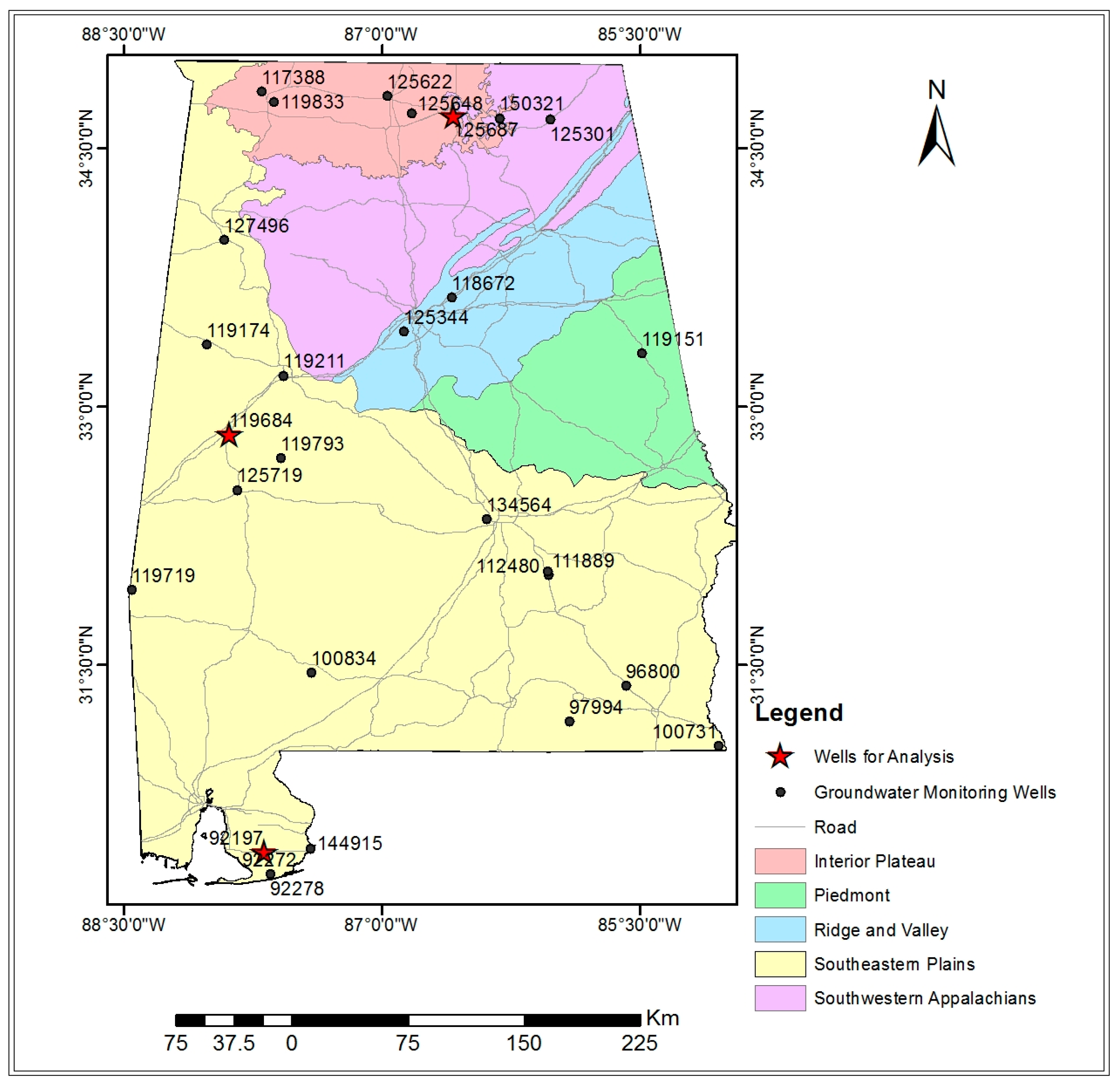
2.1. Data and Study Area

Alabama features a subtropical climate characterized by hot, humid summers and mild winters, with an average annual precipitation of approximately 55 inches (1397 mm) in the northern regions and 65 inches (1651 mm) near the coastal zone [24]. The state of Alabama is divided into five distinct hydrogeologic provinces (Figure 1), namely, the East Gulf Coastal Plain (i.e., southeastern plains), Piedmont Upland, Valley and Ridge, Cumberland Plateau, and Highland Rim [25]. These provinces are closely aligned with the state’s physiographic regions and significantly influence the dynamics and storage of groundwater. The classification of these hydrogeologic provinces is primarily based on variations in rock water-bearing properties, rock type, structural geology, and physiography, all of which play a role in determining the types of aquifers present in these areas.

Daily groundwater depth readings spanning from 1 January 2000 to 28 September 2021 were collected from the Geological Survey of Alabama’s (GSA) groundwater database (https://waterstar-al.cstestsite.com/, accessed on 2 November 2022). We carefully selected three observation wells in Alabama (Figure 1) from a comprehensive dataset containing a total of twenty-seven wells. Our selection process involved a thorough analysis of depth-to-groundwater information and consideration of the wells’ geographic locations. We also considered Alabama’s varying precipitation levels, which increase from the northern to the southern regions of the state. Each of the chosen wells was verified to be unconfined, ensuring they provided a reliable representation of the local water table with minimal influence from pumping or injections, meaning they were subject to fewer anthropogenic impacts. Many records from various locations were excluded due to insufficient length or significant data gaps. In the case of one of the three selected wells, well 92197, we encountered missing data points. These gaps were addressed using a machine learning technique called long short-term memory (LSTM). Specifically, we applied the groundwater LSTM model [26], which is designed to handle missing data by incorporating both dynamic inputs such as precipitation and static inputs such as hydraulic conductivity, soil depth, soil porosity, and maximum water content. This approach enables the model to accurately capture essential hydrogeological characteristics of the aquifer.

We also gathered daily precipitation data from 1 January 2000 to 28 September 2021, from the National Oceanic and Atmospheric Administration (NOAA). NOAA manages an extensive network of climate stations throughout the study area, offering a comprehensive database of daily precipitation records and other meteorological data (accessible at https://www.ncei.noaa.gov/cdo-web/datasets, accessed on 21 April 2023). In our analysis, we meticulously selected precipitation data from the NOAA climate station nearest to each well under consideration.

To facilitate comparison, we obtained daily GWS estimates derived through the assimilation of terrestrial water storage (TWS) data from the Gravity Recovery and Climate Experiment (GRACE) and its follow-on (FO) mission into the catchment land surface model (CLSM) [27] (https://giovanni.gsfc.nasa.gov/giovanni/, accessed on 31 January 2023). The GRACE and GRACE FO (referred to as GRACE/FO) missions utilize measurements of the Earth’s gravity field to estimate TWS variations, encompassing soil moisture, groundwater, snow, and surface water. Since GRACE/FO data represent vertically integrated observations, assimilating GRACE/FO data into a land surface model is utilized to disentangle these signals into individual processes, including groundwater processes [27]. This data assimilation also enables the spatial and temporal downscaling of GRACE/FO data, which have coarse temporal and spatial scales (monthly with an effective resolution of approximately 150,000 km² [28]). The GRACE/FO GWS data used in this study were downscaled to a daily resolution with a spatial resolution of 0.25 degrees [27] and are available for the period spanning from 2003 to 2021. To gain a better understanding of groundwater dynamics, the daily GWS estimates were further processed to derive monthly changes in GWS.

2.2. Estimation of Groundwater Storage Change

We utilized the depth-to-groundwater level data to estimate changes in GWS using the WTF method. The WTF method operates on the principle that rises in groundwater levels in unconfined aquifers result from net recharge reaching the water table [18]. The change in GWS (denoted as ΔSgw) is calculated based on the following equation:

$$\mathsf{\Delta }\mathrm{S}\mathrm{g}\mathrm{w}=\mathrm{S}\mathrm{y} \mathrm{d}\mathrm{h}/\mathrm{d}\mathrm{t}=\mathrm{S}\mathrm{y}∆\mathrm{h}/∆\mathrm{t}$$

(1)

where Sy [dimensionless] is the specific yield, h [L] is the water table height, Δh [L] is the change in the water table over the time interval $∆\mathrm{t}$, and t [T] is time. Here, Δh is computed as the net change in the hydraulic head for each month, which is the difference in heads between the end and the beginning of the month. The specific yield values are estimated in the range of 0.19 to 0.21 based on a thorough review of land surface and groundwater studies by Lv et al. [29], which considered similar aquifer materials, due to the absence of local aquifer-specific information.

2.3. Hurst Exponent

The Hurst exponent (denoted as H) is a statistical measure used to analyze the long-term memory within time series data. It was developed by Harold Edwin Hurst in the 1950s for studying the Nile river’s water levels over time, particularly to optimize reservoir storage evaluations for dam sizing [22]. The Hurst exponent quantifies long-range dependence in a time series based on its autocorrelation. A value of 1 for H indicates the presence of pink noise, distinguishing it from noise series (0 < H < 1) and random walk series (H > 1) [30]. H values between 0 and 0.5 signify an anti-correlated structure, denoting an anti-persistent process, while H values between 0.5 and 1 indicate a long-term autocorrelated structure, signifying a persistent process. An anti-persistent process implies that if a series’ fluctuations decrease/increase for a period, they are likely to reverse to increasing/decreasing subsequently. Conversely, a persistent process suggests that increases/decreases are likely to be followed by further increases/decreases. In terms of the fractal structure, fast evolving fluctuations occur when H < 1, while random walks with slowly evolving fluctuations occur when H > 1. The specific case of H = 1 represents the critical transition between noises and random walks. In this study, the Hurst exponent is calculated using the detrended fluctuation analysis (DFA) method introduced by Peng et al. [31]:

$$\mathrm{F}\left(\mathrm{s}\right)~s^H$$

(2)

$$\mathrm{Y}\left(\mathrm{j}\right)={\sum }_{k=1}^i[X_k-<x>]$$

(3)

$$F_k^2\left(\mathrm{s}\right)=\frac{1}{S}{\sum }_{J=1}^L{\left(Y_{j,k}-P_{j,k}^n\right)}^2$$

(4)

$$\mathrm{F}\left(\mathrm{s}\right)={[\frac{1}{m}{\sum }_{k=1}^m{F}_k^2\left(\mathrm{s}\right)]}^{1/2}$$

(5)

In Equation (2), the scaling function, F(s), is approximately equal to the scale, s, raised to the Hurst exponent, H. Equation (3) computes a cumulative sum (Y) where X_k denotes a specific value and <x> represents the mean of the time series. Equation (4) determines the variance (F²) of each section by subtracting a best-fit polynomial of order, n (Pⁿ). Finally, Equation (5) calculates the square root of the average variance for all segments, which defines the scaling function. Different values of the Hurst exponent, H, indicate distinct properties in a system. In this investigation, H is calculated within the range of 0 to 1.

We examined the transition of the scaling structure among the factors through the distribution of the timescale local Hurst exponent (TS–LHE). The probability density function (PDF) of the local Hurst exponent (LHE) is constructed using the Gaussian kernel method, as outlined below:

$$g\left(h\right)=\frac{1}{\sqrt{2\pi \sigma }}exp\left[-\frac{{\left(h-H_0\right)}^2}{2{\sigma }^2}\right]$$

(6)

where $\sigma$ denotes the standard deviation of H and H₀ represents the mean exponent. We define the main Hurst exponent, $\overline{H}$, as the LHE corresponding to the maximum of the PDF. The resulting PDF is then plotted on a semi-logarithmic coordinate system to better facilitate a more detailed examination of its tailing characteristics [32].

2.4. Integrated Time-Series Techniques and Trend Analysis

In this study, we also employ time-series and trend analysis methods to discern underlying patterns and relationships within the hydrologic and climate data. These integrated techniques include the seasonal-trend decomposition procedure based on Loess (STL), the Mann–Kendall significance test, Thiel–Sen’s slope, and wavelet analysis, each of which is briefly described below.

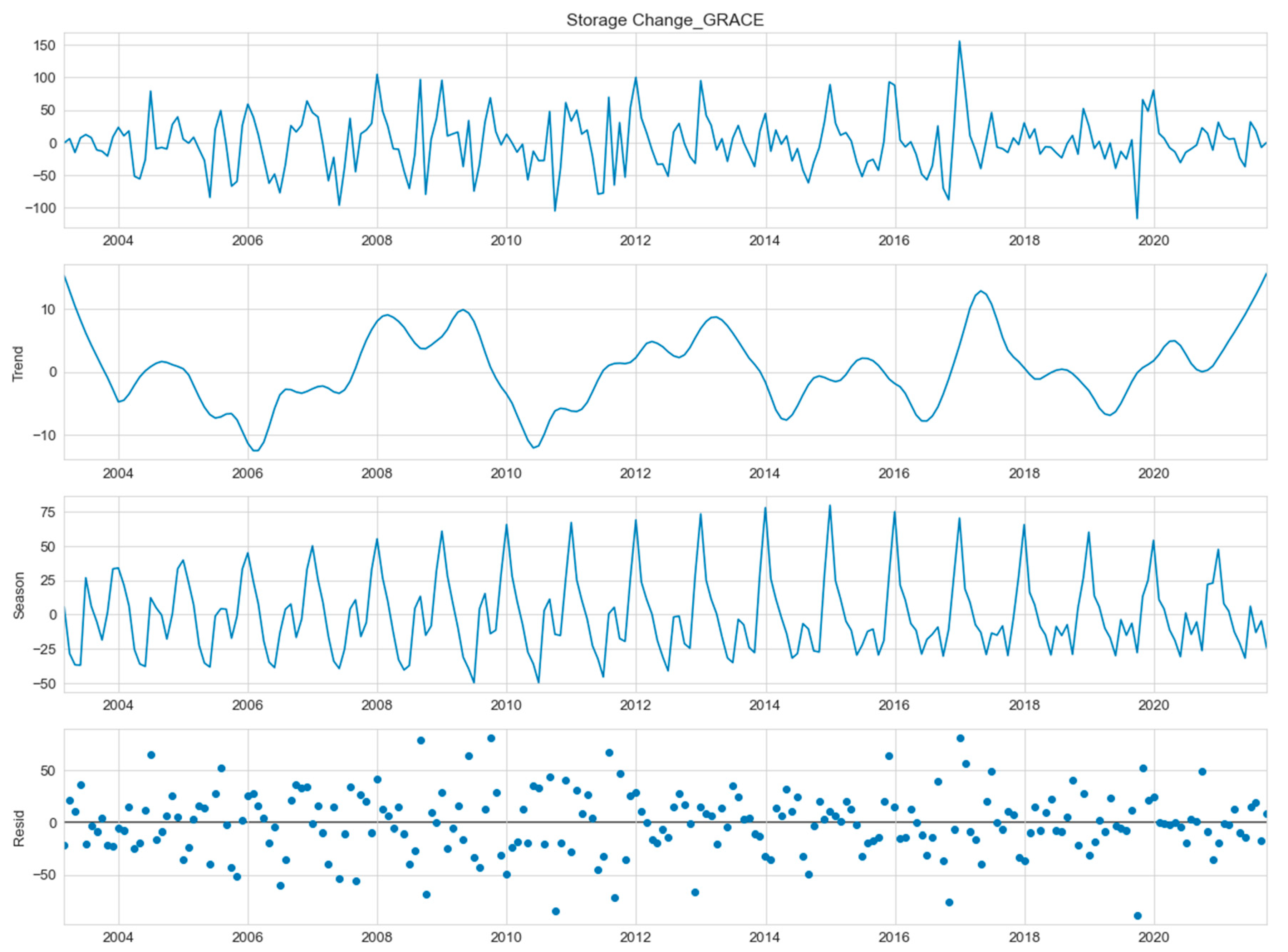
2.4.1. Time Series Decomposition and Trend Analysis

To gain a deeper insight into the trends in GWS changes, we employed the STL, as detailed in Appendix A. STL is considered one of the most effective methods for dissecting variations in time data series across various temporal scales [33,34]:

GWS_obs = GWS_trend + GWS_seasonal + GWS_residual

(7)

where GWS_trend represents the long-term trend component, GWS_seasonal denotes the seasonal cycle, and GWA_residual is the residual component.

We determined the trends in GWS changes for our study site using the Mann–Kendall test and Thiel–Sen’s slope [33]. The non-parametric Mann–Kendall (MK) trend test is a commonly employed method for evaluating the statistical significance of monotonic trends in hydro-meteorological time series. In this study, we employed the MK test to assess the trends in groundwater storage and precipitation. Thiel–Sen’s slope offers an accurate trend estimation without the need for specific data distribution assumptions and with minimal sensitivity to outliers. By organizing the data based on the time variable, calculating differences between dependent variable values at different time points, and computing slopes for each pair of differences, the resulting median slope provides a robust estimate of the overall trend or rate of change in the time series. This non-parametric approach ensures reliable trend estimation that remains resilient to outliers and accounts for unknown data distributions. The application of Thiel–Sen’s slope estimation to our time series dataset yields precise trend estimation, enhancing the robustness and accuracy of our analysis by mitigating the influence of outliers and avoiding assumptions about the data distribution.

2.4.2. Wavelet Analysis

Wavelet analysis is a potent time-frequency method that enables examining data across various scales and resolutions [35]. Through the decomposition of the time series into wavelet components, we can identify and characterize local variations, transient features, and trends within the data. This method is particularly useful for detecting patterns and anomalies in non-stationary data, such as precipitation and GWS changes considered in our study. It is noteworthy that hydrologists have used wavelet analysis to uncover complex relationships at various scales and locations. For instance, Si et al. [36] used wavelet coherence analysis to show how saturated hydraulic conductivity relates to soil properties such as sand content and organic carbon content at different scales and locations. Lu et al. [37] applied wavelet analysis to understand spatial patterns and controls on deep soil bulk density, such as soil depth, magnetic susceptibility, organic carbon, and particle size composition. These successful applications inspire us to use cross-wavelet and wavelet coherence to explore potential correlations between GWS changes and precipitation. In future studies, we aim to investigate GWS changes in relation to multiple potential drivers.

3. Results

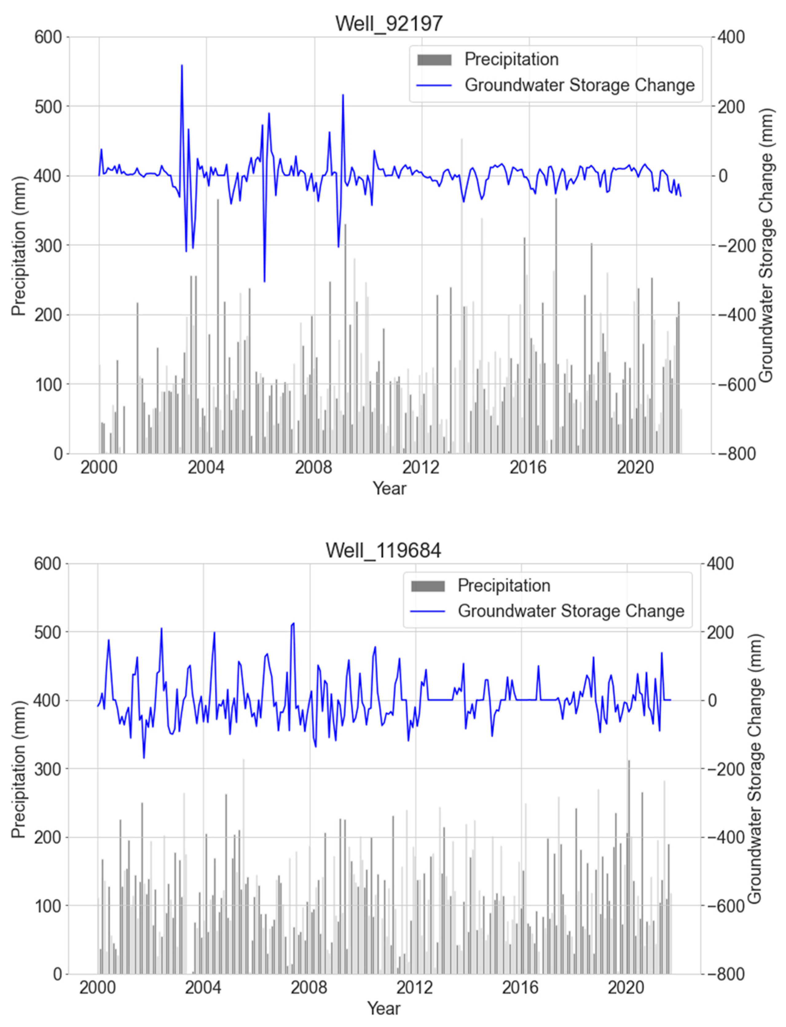
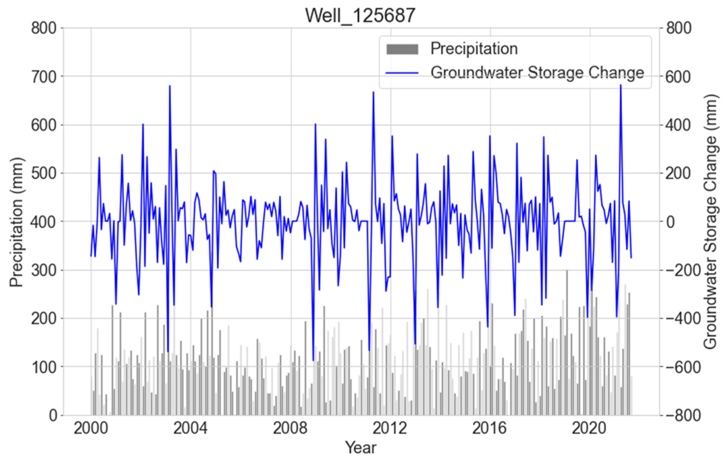
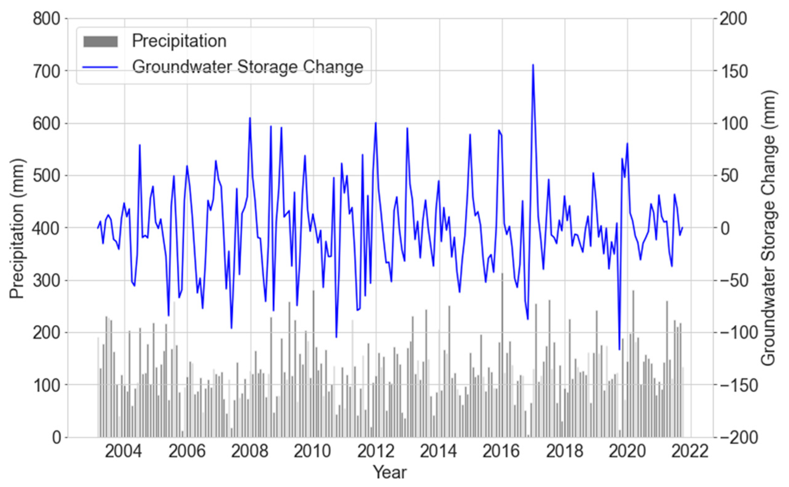
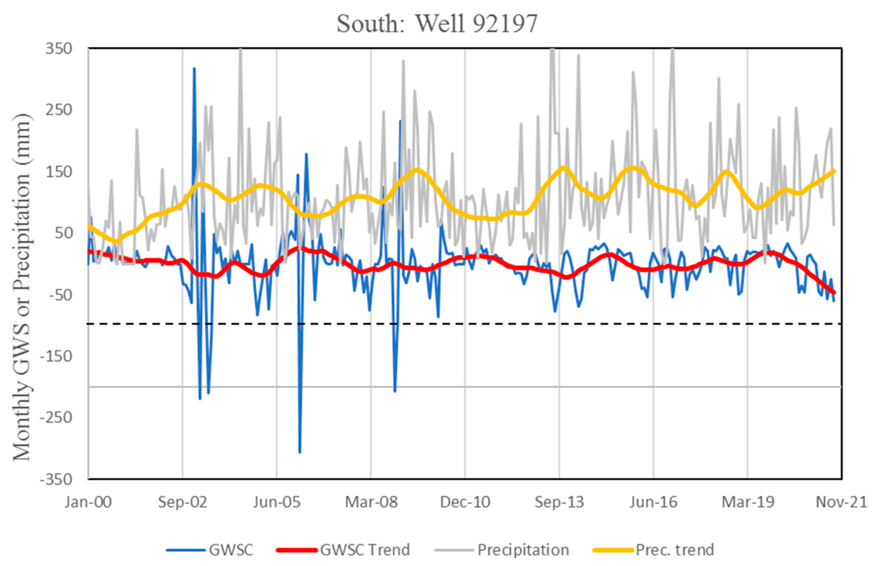
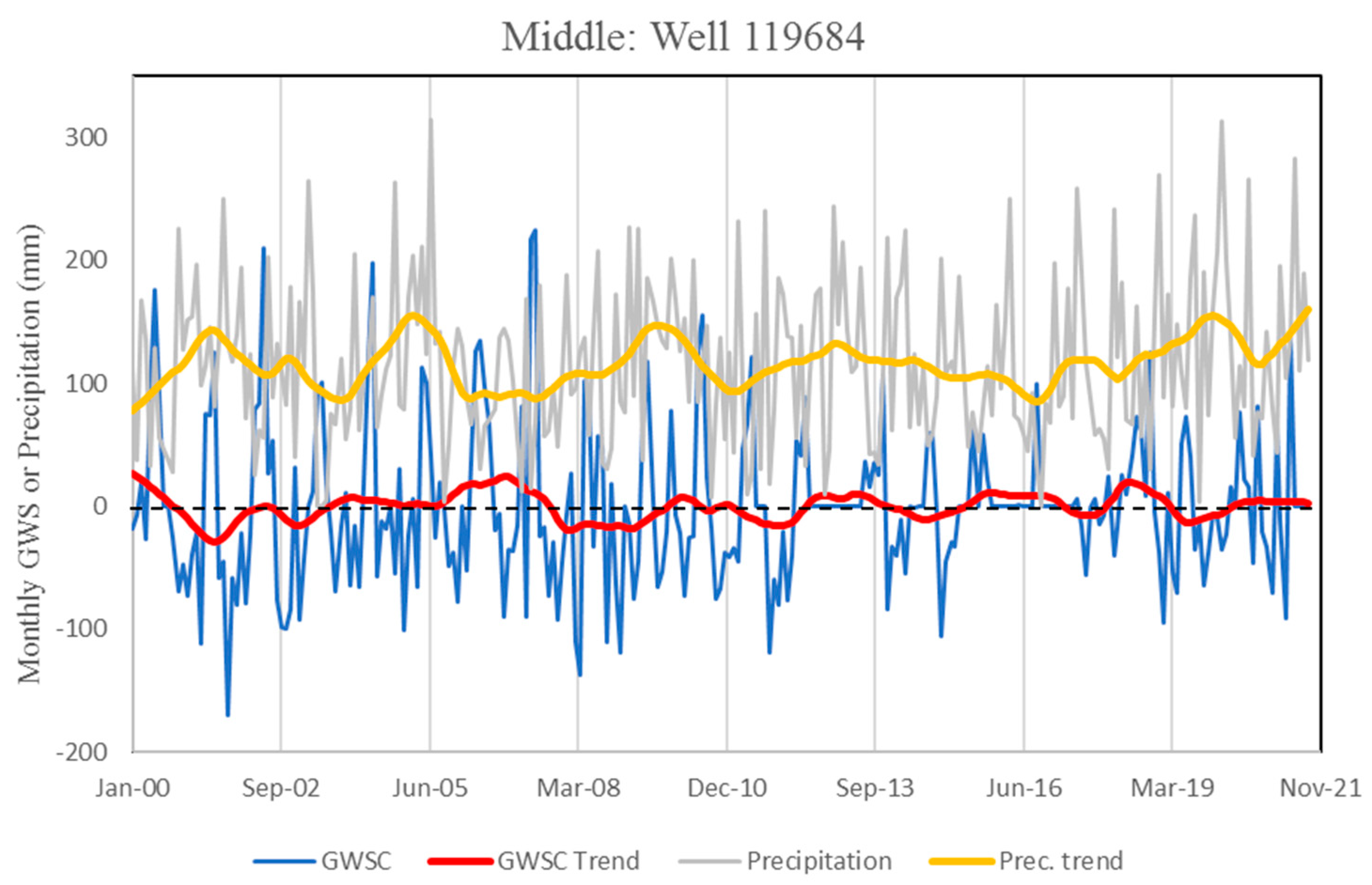
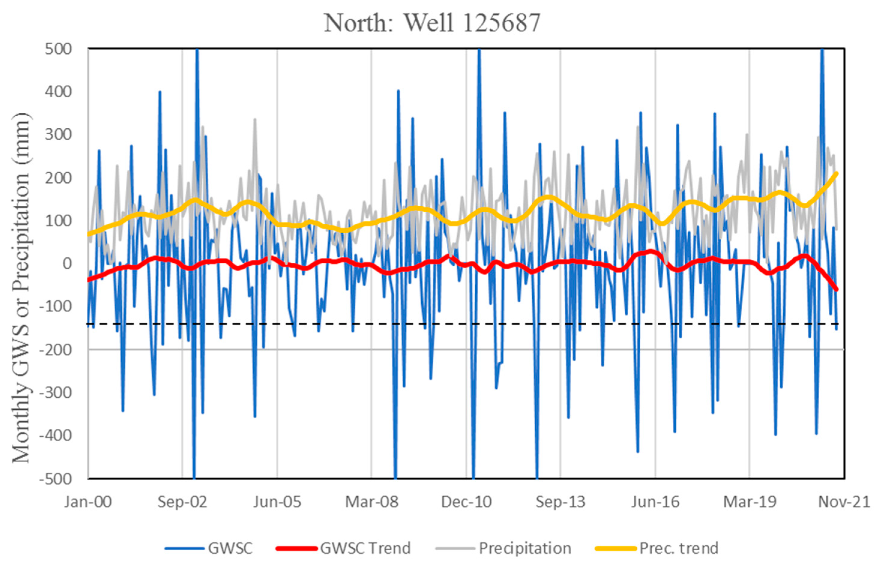
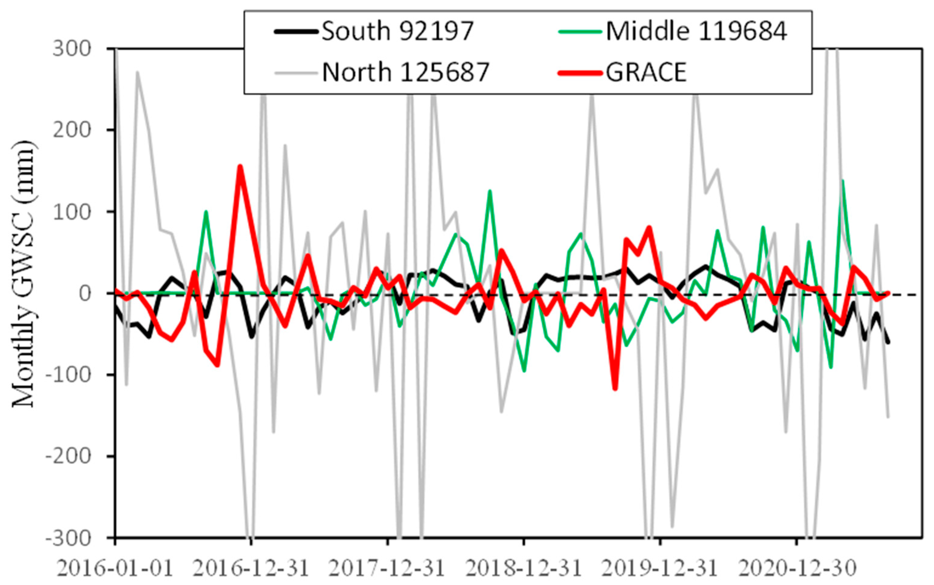
3.1. Groundwater Storage Changes and Trend Analysis

Figure 2 illustrates the evolution of monthly GWS changes (estimated using the WTF method) and precipitation from 2000 to 2021 for the three selected representative wells, as shown in Figure 1. In each plot, the upper curve (represented by the blue line) displays the temporal changes in GWS, revealing distinct fluctuation patterns for each well sited in a different region in the state of Alabama. This direct comparison within the same timeframe provides a compelling visual representation of their interconnectedness. We created a spatiotemporal map (refer to Figure A2 in Appendix B) using GWS change data estimated from 27 monitoring wells. This map visually illustrates annual changes in GWS across Alabama from 2000 to 2021 (further details can be found in Appendix B).

Figure 3 displays the GWS changes estiamted for Alabama using the GRACE/FO data assimilation alongside the area-averaged precipitation data. The monthly state-wide GWS changes reveal October 2016 as one of the driest months (with a state-wide GWS change of −87 mm), coinciding with the severe to extreme drought that affected much of the Southeastern U.S. throughout 2016. Another noteworthy observation is the driest month in August 2019, marked by a GWS decrease of −120 mm. Interestingly, these dry conditions, while significant at the state-wide level, were not reflected in the data from the three individual wells depicted in Figure 2. This discrepancy will be explained below in the discussion section.

Expanding upon these observations, Figure 4, Figure 5, Figure 6 and Figure 7 offer a more detailed analysis, showcasing the trends in changes in GWS and precipitation at the three distinct wells across Alabama: Well 92197 in the southern region, Well 119684 in the western region, and Well 125687 in the northern region. Although the Mann–Kendall test (as detailed in Appendix C) did not reveal statistically significant trends at a 90% confidence level for these wells, Sen’s slope analysis did detect subtle changes. Well 92197, situated near the coastline, showed a marginal decrease in GWS, indicated by a negative Sen’s slope of −0.20 mm/yr. In contrast, the western region (Well 119684) exhibited an increase, with a positive Sen’s slope of 0.50 mm/yr, more than two times larger than the GWS loss observed in the south. Well 125687 in the northern region also showed a minor increase in GWS, with a Sen’s slope of 0.38 mm/yr. A similar analysis was applied to the precipitation data, revealing a range of Sen’s slopes: 0.08 mm/yr, 0.018 mm/yr, and 0.08 mm/yr for Well 92197, 119684, and 125687, respectively. These results suggest an overall increasing trend of monthly precipitation across Alabama, with slightly more precipitation in the south than in the north, consistent with historical trends. These trends underscore regional variations in both GWS changes and precipitation and highlight distinct spatiotemporal evolution patterns between GWS changes and precipitation. This complexity indicates the multifaceted response of groundwater systems to climate change in Alabama.

Furthermore, the analysis of area-averaged precipitation data for Alabama, as depicted in Figure 7, revealed a moderate increase, with a Sen’s slope of 0.033 mm/yr. Meanwhile, the GRACE GWS change data exhibited a positive trend of 0.002 mm/yr, indicating a generally increasing trend across the state of Alabama in the last two decades. Notably, this trend is one order of magnitude less than the increasing trend observed in average precipitation. It is worth noting that approximately 10% of precipitation is believed to infiltrate into aquifers in Alabama).

Figure 8 shows time series of monthly GWS changes at the three wells in comparison to the average GRACE/FO GWS change data at the three well locations. One of the initial observations is the marked difference in the magnitude of GWS changes. Furthermore, the well measurements display more significant fluctuations when contrasted with the GRACE/FO GWS change data. These discrepancies can likely be attributed to variations in spatial scale, the model’s limitations in capturing finer-scale subsurface property variability, such as hydraulic conductivity, and the utilization of coarse-scale forcing fields to drive model simulations.

It is crucial to consider that variables such as pumping rates, recharge patterns, and geological structures may impact GWS changes at the point scale (i.e., at the observation well). The heterogeneity of these factors across different locations can lead to substantial variations in GWS changes, even over relatively short distances. Since these variables may not be adequately captured in the coarse-scale GRACE/FO GWS and the land surface model, this could potentially explain the discrepancies observed between the GRACE/FO data and well measurements in Figure 8.

We also conducted a comparison between the GWS change results from the WTF method and a process-based numerical model obtained from Ponprasit et al. [38]. The comparative results can be found in Appendix D, showing that the WTF method applied by this study is reliable.

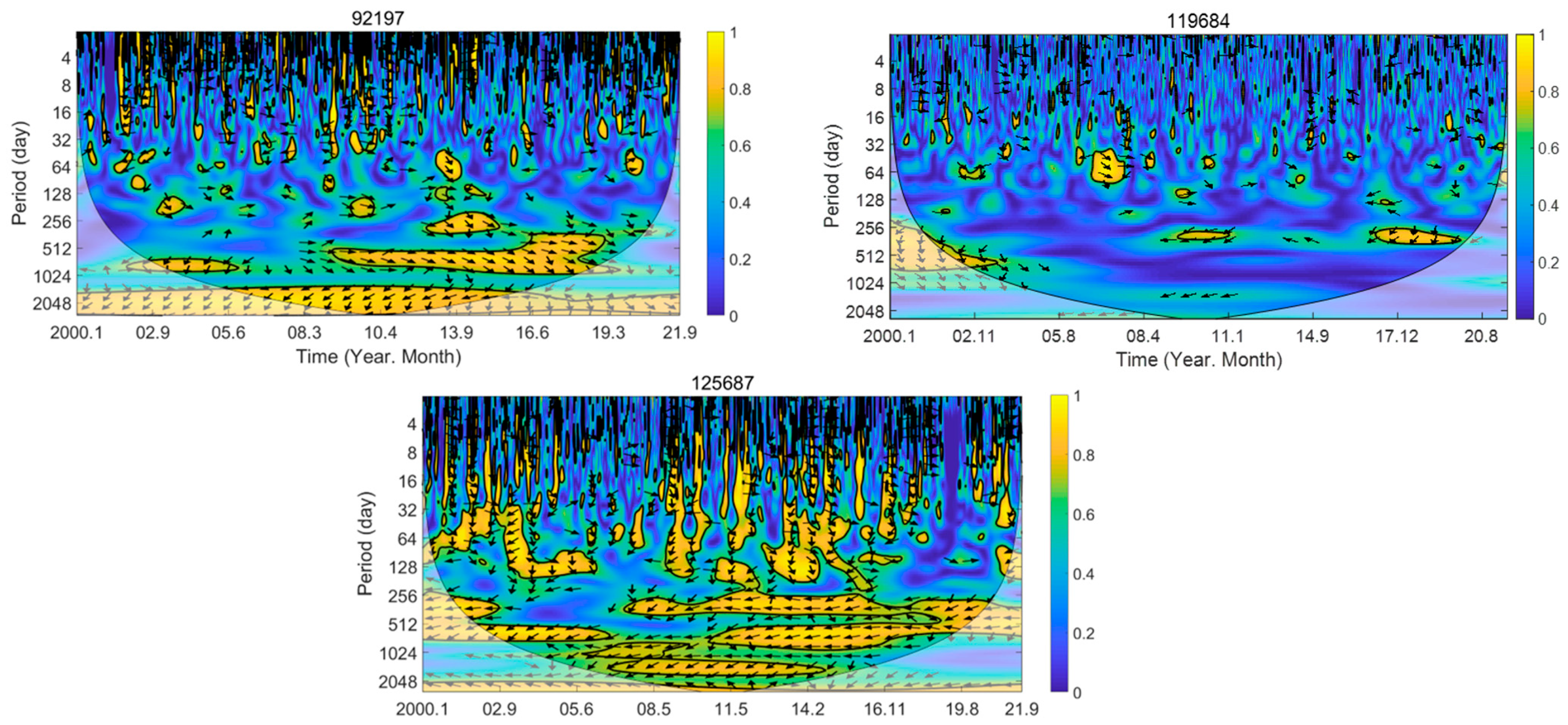
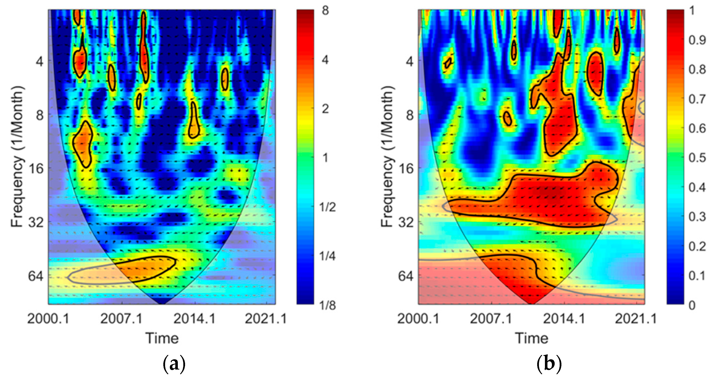
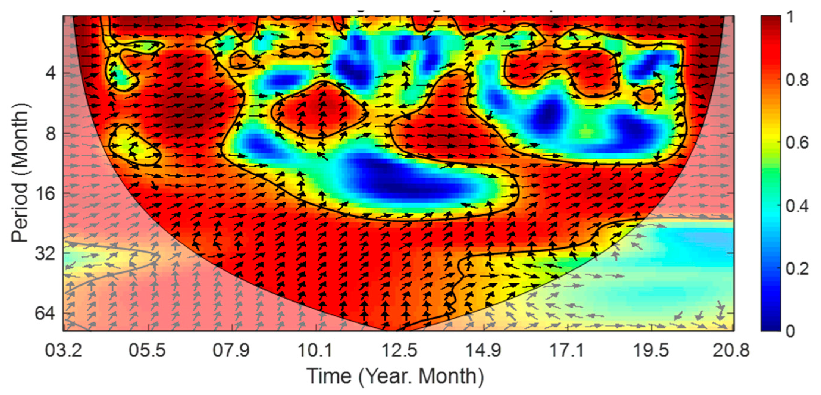
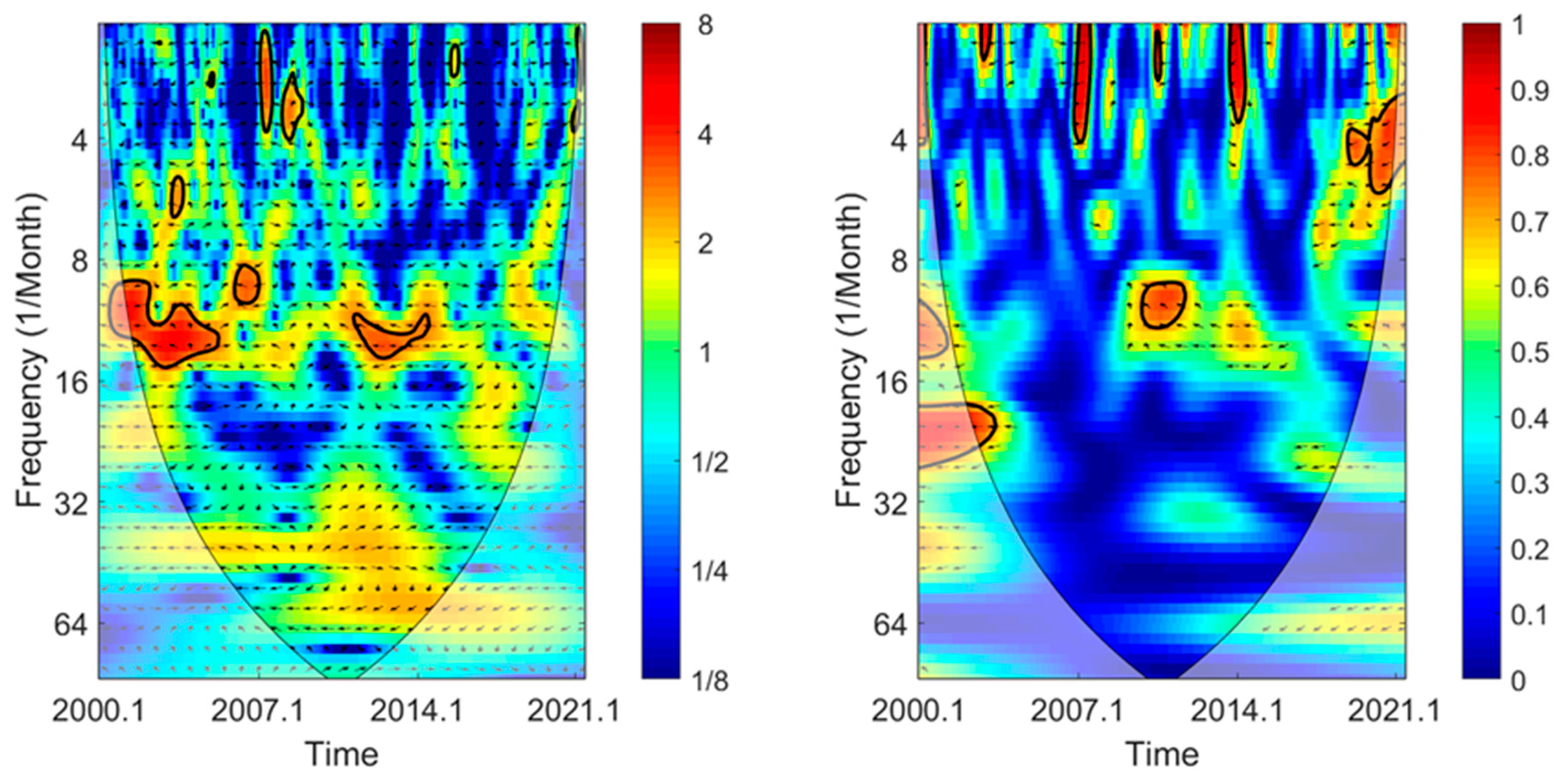
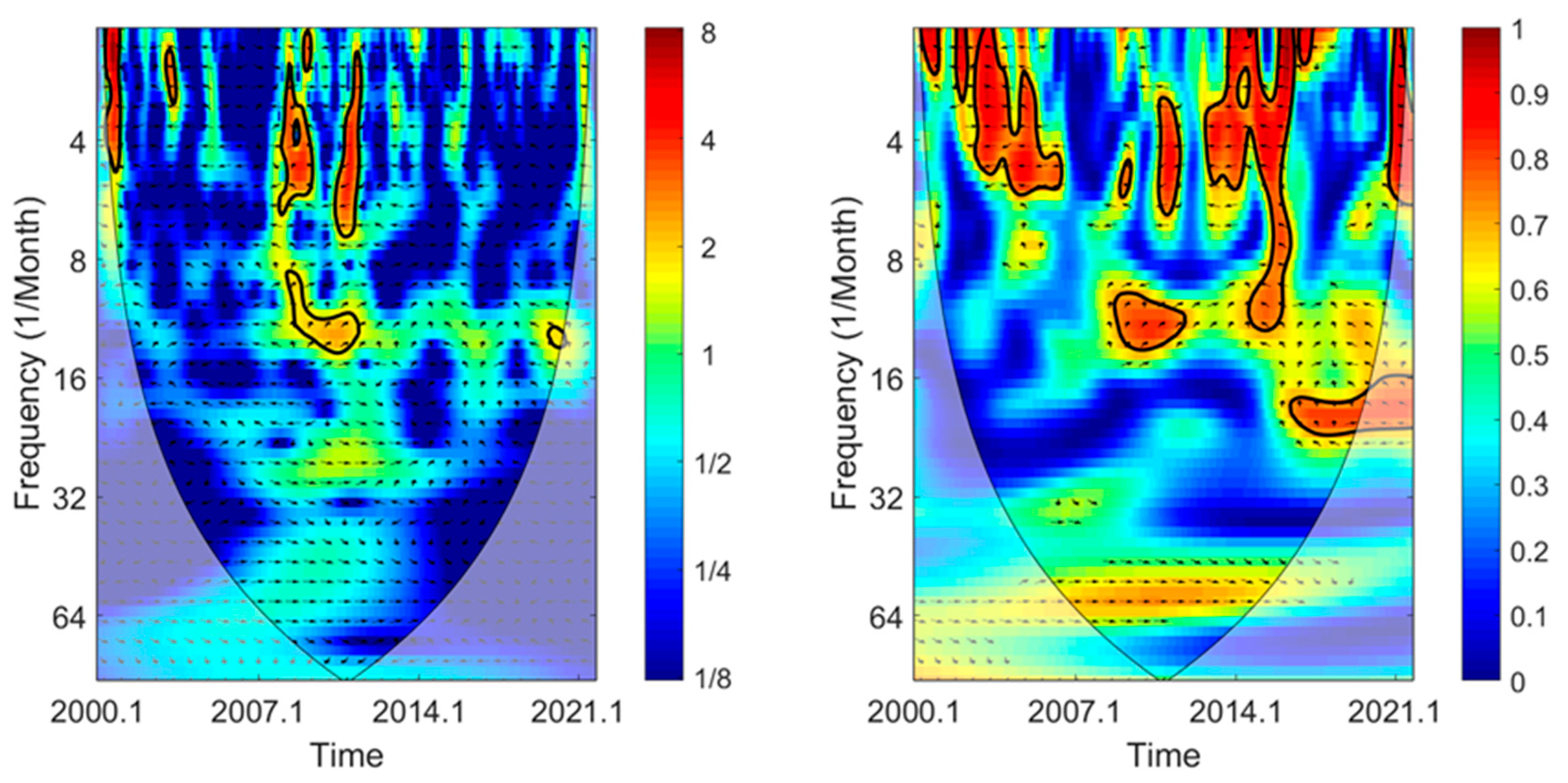
3.2. Wavelet Analysis

Figure 9 illustrates the wavelet coherence between precipitation and groundwater depth at the three well locations. The wavelet coherence In the case of Well 92197, a pronounced covariance (depicted in yellow) is evident for periods exceeding 512~1024 days and persists over multiple years. This suggests a robust correlation between precipitation and water depth on time scales longer than 512~1024 days. The covariance appears to be sporadic in the 256–512-day range, and synchronization between water depth and rainfall is more fragmented on an annual basis. In the case of Well 119684, the area demonstrating high covariance between precipitation and water depth is relatively limited. Notable coherence is sporadically observed across both monthly and yearly time scales. Finally, for Well 125687, the results reveal a clear correlation between water depth and rainfall throughout the study duration. The most significant areas of coherence predominantly occur in periods shorter than 128 days, as well as in the annual and 1024–2048 day ranges.

Figure 10 shows that GWS change and precipitation do not exhibit the regular characteristics of strong coherence at Well 92197 (Figure 10a). However, there is noticeable co-variation between the GWS change and precipitation over a period of 16~32 months (Figure 10b). Moreover, similar phase (anti-phase) characteristics are observed in regions that pass the significance test. In addition, variations in the relationship between GWS and precipitation are evident over periods of less than one year at different times. For further insights into the wavelet analysis results for Well 119684 and Well 125687, please refer to the cross wavelet and wavelet coherence spectrum provided in Appendix E (Figure A4 and Figure A5). These results do not display the typical patterns or characteristics observed in such analyses, suggesting a lack of clear correlation between the GWS changes and precipitation for these two wells.

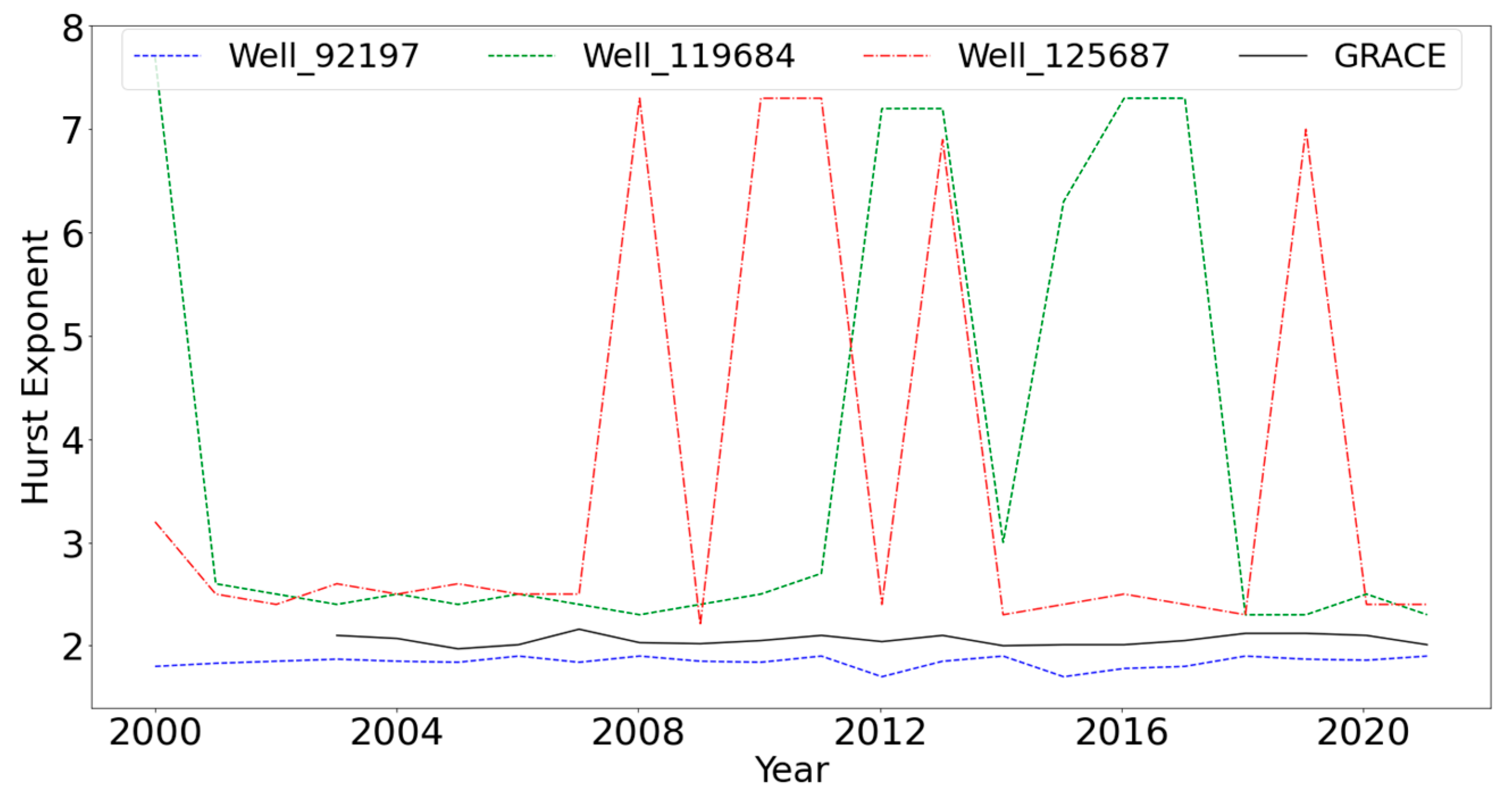
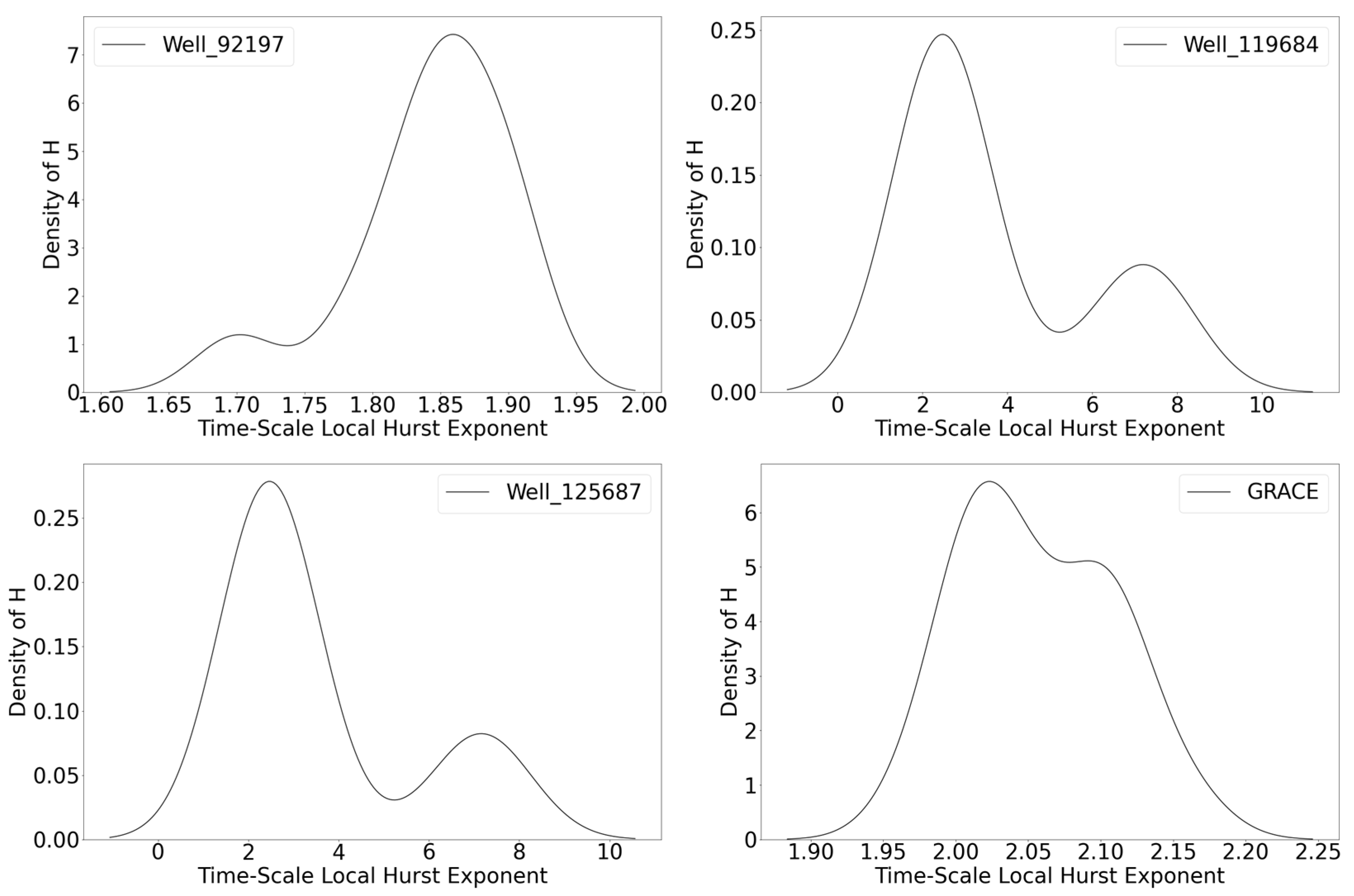
3.3. Time-Scale Local Hurst Exponent

In this study, we computed the time-scale local Hurst exponents for each well and the GRACE/FO GWS changes to investigate their comparative dynamics. The total period of investigation was divided into twenty-two discrete intervals, each approximately one year in duration, starting on 1 June 2000 and ending on 30 September 2021. Within these intervals, we detected notable variations in the main Hurst exponent ($\overline{H}$). In certain years, $\overline{H}$ exceeded 1.0, showing strong persistence within the well data. In contrast, during other years, $\overline{H}$ fell below 1.0, indicating less persistent behavior. Higher $\overline{H}$ values during certain periods underscore the presence of long-range dependence or memory within each system. Figure 11 and Figure 12 visually illustrate these fluctuations in the Hurst exponent over the twenty-two-year span for the three wells and the GRACE GWS changes.

The results of the wavelet coherence analysis reveal significant correlations between the trend of precipitation (area-averaged) and GWS change using GRACE/FO data. In Figure 13, the darker region above the significance contours highlights these notable coherence values. The phase relationship, depicted by the arrows, provides additional insights: rightward arrows indicate an in-phase relationship, suggesting that changes in precipitation coincide with corresponding changes in GWS (most arrows in Figure 13 follow this direction). Conversely, leftward arrows indicate an anti-phase relationship, indicating opposing changes in precipitation and GWS changes.

The coherence values presented in

Table 1. The average coherence between the trend of the precipitation and groundwater storage changes (using GRACE/FO GWS data) at different scales. In the legend, “all scales” means the average value at all scales (in units of month).

<4	4–8	8–16	16–32	32–64	>64	All Scales
0.7139	0.6832	0.6487	0.7558	0.7066	0.7522	0.7042

further support these findings. For instance, the average coherence value at the scale of <4 months is 0.7139, indicating a moderate to strong correlation between the precipitation trend and GWS change at that specific time scale. Similar interpretations apply for the average coherence values at other scales.

4. Discussion

4.1. Groundwater Storage Trends

The Mann–Kendall test results indicated no significant trend in GWS change for all wells, including Well 119684 in the western region, or the GRACE data. This suggests that the overall trend of GWS changes might be static across the state or vary too randomly to discern a clear trend. However, this result should not be interpreted as implying that no changes are occurring. On the contrary, a more detailed analysis using the Sen’s slope method revealed a different perspective. In the southern region, Well 92197 displayed a negative Sen’s slope for GWS change (−0.20 mm/yr), implying a possible gradual depletion of the groundwater resource in southern Alabama. This is concerning given the necessity of groundwater for both anthropogenic activities and natural systems in the region. This decline points to a potential mismatch between groundwater recharge and withdrawal rates, with withdrawals possibly exceeding the natural replenishment. Interestingly, the Sen’s slope for precipitation at this location showed a positive trend (0.08 mm/yr). This finding somewhat contradicts the common expectation that increased precipitation would naturally lead to an augmentation in GWS [39]. Therefore, the continuous decrease in GWS at this location implies the possible impacts of other external factors. For example, anthropogenic factors such as increased groundwater pumping for irrigation, industrial usage, or urban water supply could be contributing to the decrease in GWS [40,41]. Additionally, changes in land use and land cover, as well as alterations to the natural drainage patterns, could also affect the groundwater recharge capacity of the area, leading to a decline in GWS even with increased precipitation.

Well 119684 in the western region tells a different story, with a positive Sen’s slope for GWS changes (0.50 mm/yr). The rise in GWS suggests an effective balance between recharge and withdrawal processes, leaning towards a surplus. However, a curious observation is that the Sen’s slope estimate for precipitation is notably lower (0.018 mm/yr), indicating a less pronounced positive trend. This inconsistency hints at the influence of factors other than precipitation in boosting groundwater storage. It is possible that changes in land use, decreased extraction, and/or geological factors are enhancing groundwater recharge or reducing withdrawals, leading to the observed increase in GWS.

In the northern region, Well 125687 shows a modest positive Sen’s slope for GWS (0.38 mm/yr). This upward trend in GWS aligns with the observed Sen’s slope for precipitation (0.08 mm/yr), suggesting that rainfall might be playing a crucial role in augmenting the groundwater reservoir in this area.

The comparison of individual well data with the area-averaged GRACE GWS change data (Sen’s slope: 0.033 mm/yr) for Alabama reveals a critical aspect of groundwater dynamics in the state. The trends observed for Well 119684 and Well 125687 closely align with the trends in the area-averaged GRACE GWS changes, indicating a degree of regional consistency. However, Well 92197 in the southern region deviates from this regional pattern, again pointing to the significance of local site-specific factors in groundwater dynamics.

4.2. Response of Groundwater Storage to Climate Change

The analysis of the relationship between GWS changes and precipitation at Well 92197 reveals a complex interplay between these two variables. These findings have important implications for understanding the impact of climate variability on groundwater resources. Climate variability, including changes in precipitation patterns and intensity, can significantly impact GWS [42,43]. However, based on wavelet analysis, the results do not consistently indicate strong coherence between these factors, indicating that the dynamics of GWS change at this location may not be directly and predictably tied to precipitation data. This observation raises the possible influence of other unidentified factors or a more complex underlying process. Nevertheless, our analysis also identified periods of 8 to 32 months where GWS changes and precipitation significantly co-varied. This result suggests that peaks in precipitation might correspond to minimum GWS levels, implying a lag time of approximately half the observed cycle (16 months). This lag time signifies the response of GWS changes to precipitation.

Regarding phase characteristics, we observed both in-phase and anti-phase patterns within the dataset, indicating that GWS and precipitation can sometimes move in the same direction and other times in opposing directions. This variability further demonstrates the complexity of the relationship between these two variables and suggests that different factors or mechanisms might influence them at different times. In our wavelet coherence analysis, we discovered that the strongest and most consistent co-variability between GWS changes and precipitation occurred over a period of 8 to 32 months. This highlights the potential importance of multi-year climatic or hydrological cycles in driving changes in both GWS and precipitation. Contrarily, Appendix E, which depicts the cross-wavelet and wavelet coherence spectrum, does not show regular characteristics or patterns. The lack of clear patterns suggests that the relationship between GWS changes and precipitation is more complex and likely dependent on additional variables or conditions, which need to be identified in future studies.

4.3. Time-Scale Local Exponent and System Memory

The significant fluctuation of the Hurst exponent, $\overline{H}$, across the study period (2000~2021) reveals intricate dynamics within both the well and GRACE datasets. The instances where $\overline{H}$ exceeded 1.0 signify strong persistence, implying that previous states in these systems exert a considerable influence on future states. This persistent behavior reflects a long-range dependence or memory within these systems, where present and future values show significant correlations with historical data. Interestingly, the variation in the Hurst exponent over time challenges the traditional assumption of stationary dynamics, revealing a significant temporal component to the system’s dynamics [44].

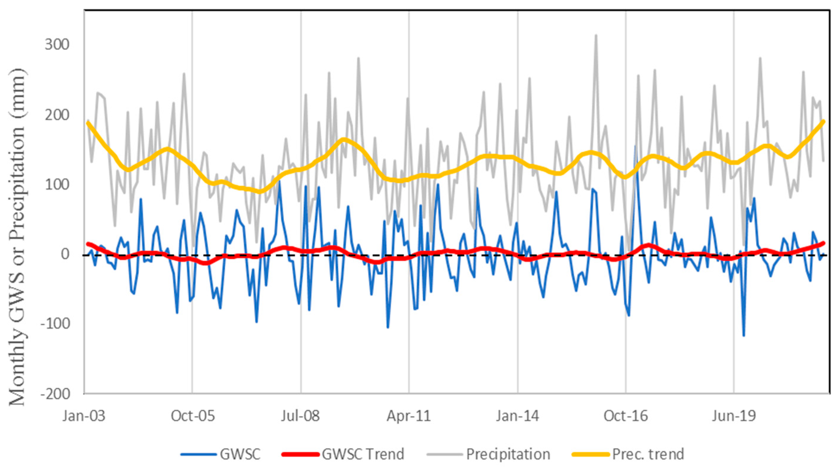
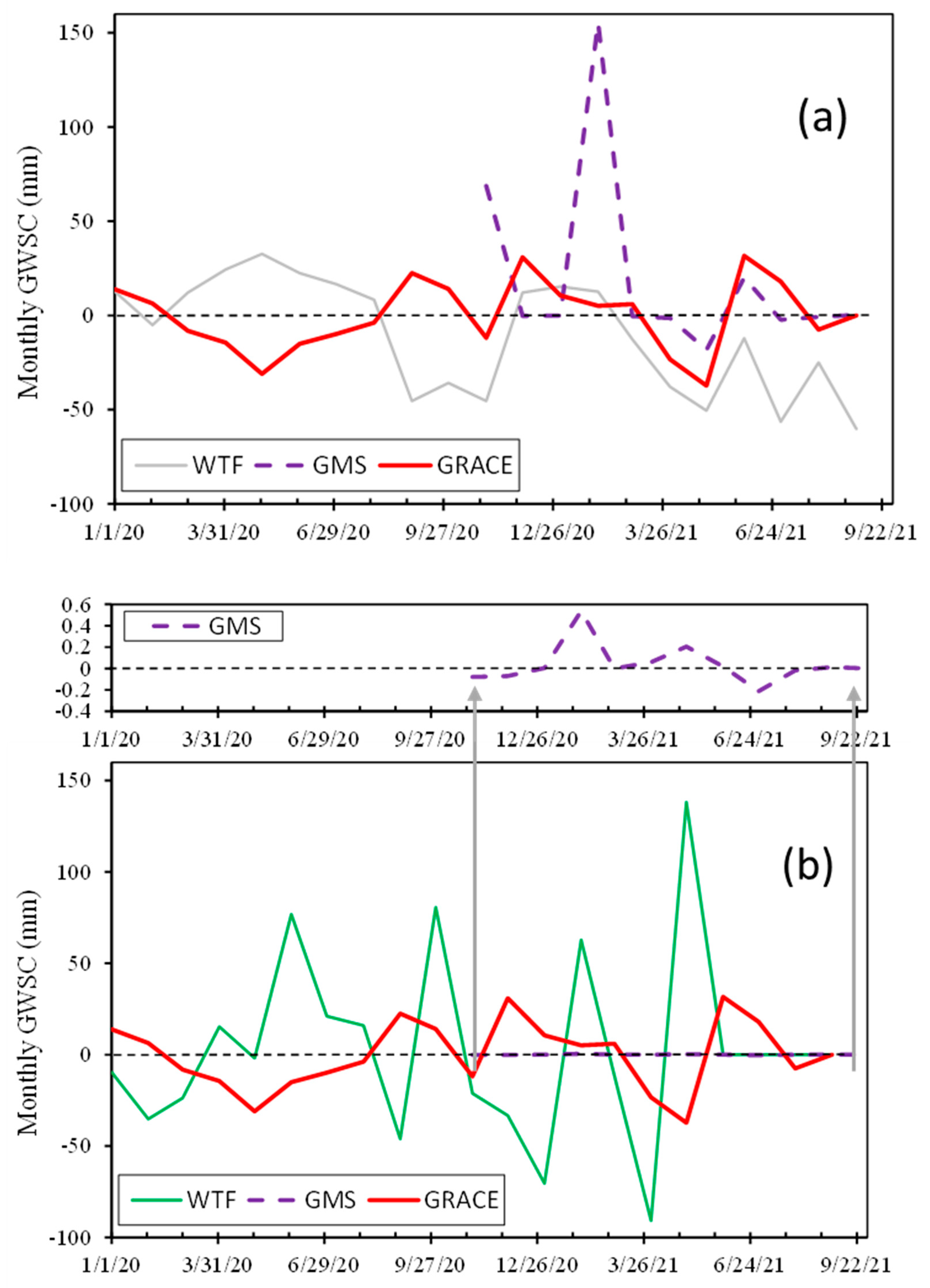
4.4. Comparison between GWS Changes Derived from Wells and GRACE/FO Data Assimilation

Groundwater level observations provide a microscale perspective, offering intricate insights into localized changes with fine details. In contrast, GRACE/FO GWS data depict changes in GWS at a much larger spatial scale (0.25°). Consequently, GRACE GWS data represent averaged variability, which inherently may not capture localized anomalies accurately. While this large-scale perspective is valuable for identifying broader trends and patterns, it might have limitations in accurately capturing localized nuances, resulting in less high-frequency variability in GWS changes when compared to well data.

Further exacerbating these disparities are the distinct methodologies employed by the WTF and GRACE/FO data assimilation. WTF relies on direct observations of water levels at specific locations, providing precise and highly localized measurements. This level of detail enables the detection of subtle variations and fluctuations in GWS, contributing to the higher magnitude of changes observed in the well data. In contrast, GRACE/FO GWS estimates were derived by assimilating coarse-scale satellite measurements into a land surface model that has not been calibrated using well data. The precipitation and other atmospheric forcing fields used to drive GRACE/FO data assimilation were derived from re-analysis outputs, which may not capture precipitation variability at individual well locations [27]. Consequently, GRACE/FO GWS may not as effectively discern minor localized changes as direct observations. Additionally, the coarse-scale nature of GRACE/FO data cannot identify smaller-scale variations as observed by individual wells.

5. Conclusions

This study revealed a nuanced relationship between groundwater storage trends and their responses to climatic changes in the state of Alabama. Despite the initial absence of an evident trend in groundwater storage across all locations, a deeper analysis indicated a complex scenario with trends exhibiting considerable variation. This variability underscores the influence of factors beyond precipitation, including local recharge, pumping rates, and geological conditions, all of which may significantly affect groundwater storage dynamics. Moreover, the findings suggested a multifaceted interaction between groundwater storage changes and precipitation. This interplay did not exhibit consistent correlation; however, it did reveal certain intervals of significant co-variability, hinting at possible cyclic or intermittent influences that merit further investigation. The variability in phase patterns and the strong periodicity observed in the data might indicate the impact of seasonal changes, though more detailed studies are necessary to confirm these hypotheses.

Furthermore, the local Hurst exponent identified the presence of strong persistence within the groundwater system. This persistence implies a high degree of correlation between current, future, and historical data, thus indicating the system’s memory. The temporal variability in this Hurst exponent challenges the traditional assumption of stationary dynamics, highlighting a substantial temporal component in the system’s behaviors.

In conclusion, this study demonstrated the high complexity in groundwater storage dynamics and its correlation with climate variables. Recognizing and comprehending these complex dynamics is essential for the development of effective and sustainable groundwater management strategies, particularly with increasing climate variability and change. Further research should focus on a more profound exploration of these relationships, the potential cyclic or intermittent influences, and the effects of other environmental and human-induced factors.

References

1. Calow, R.C.; MacDonald, A.M.; Nicol, A.L.; Robins, N.S. Ground water security and drought in Africa: Linking availability, access, and demand. Groundwater 2010, 48, 246–256. [Google Scholar] [CrossRef]
2. Martirosyan, A.V.; Ilyushin, Y.V.; Afanaseva, O.V. Development of a distributed mathematical model and control system for reducing pollution risk in mineral water aquifer systems. Water 2022, 14, 151. [Google Scholar] [CrossRef]
3. Martirosyan, A.V.; Kukharova, T.V.; Fedorov, M.S. Research of the hydrogeological objects’ connection peculiarities. In Proceedings of the 2021 IV International Conference on Control in Technical Systems (CTS) 2021, Saint Petersburg, Russia, 21–23 September 2021; pp. 34–38. [Google Scholar]
4. Pershin, I.M.; Papush, E.G.; Kukharova, T.V.; Utkin, V.A. Modeling of Distributed Control System for Network of Mineral Water Wells. Water 2023, 15, 2289. [Google Scholar] [CrossRef]
5. Naga Rajesh, A.; Abinaya, S.; Purna Durga, G.; Lakshmi Kumar, T.V. Long-term relationships of MODIS NDVI with rainfall, land surface temperature, surface soil moisture and groundwater storage over monsoon core region of India. Arid. Land Res. Manag. 2023, 37, 51–70. [Google Scholar] [CrossRef]
6. Asif, Z.; Chen, Z.; Sadiq, R.; Zhu, Y. Climate change impacts on water resources and sustainable water management strategies in North America. Water Resour. Manag. 2023, 37, 2771–2786. [Google Scholar] [CrossRef]
7. Krishan, G.; Patidar, N.; Sudarsan, N.; Vasisth, R.; Sidhu, B.S. Groundwater Responses to Climate Variability in Punjab, India. In Climate Change and Environmental Impacts: Past, Present and Future Perspective; Springer International Publishing: Cham, Switzerland, 2023; pp. 333–343. [Google Scholar]
8. Meixner, T.; Manning, A.H.; Stonestrom, D.A.; Allen, D.M.; Ajami, H.; Blasch, K.W.; Walvoord, M.A. Implications of projected climate change for groundwater recharge in the western United States. J. Hydrol. 2016, 534, 124–138. [Google Scholar] [CrossRef]
9. Shah, T. Climate change and groundwater: India’s opportunities for mitigation and adaptation. Environ. Res. Lett. 2009, 4, 035005. [Google Scholar] [CrossRef]
10. Dale, V.H.; Efroymson, R.A.; Kline, K.L. The land use-climate change-energy nexus. Landsc. Ecol. 2011, 26, 755–773. [Google Scholar] [CrossRef]
11. Yasarer, L.M.; Taylor, J.M.; Rigby, J.R.; Locke, M.A. Trends in land use, irrigation, and streamflow alteration in the Mississippi River Alluvial Plain. Front. Environ. Sci. 2020, 8, 66. [Google Scholar] [CrossRef]
12. Hou, Q.; Pei, T.; Yu, X.; Chen, Y.; Ji, Z.; Xie, B. The seasonal response of vegetation water use efficiency to temperature and precipitation in the Loess Plateau, China. GECCO 2022, 33, 01984. [Google Scholar] [CrossRef]
13. Tran, A.P.; Dafflon, B.; Hubbard, S.S.; Kowalsky, M.B.; Long, P.; Tokunaga, T.K.; Williams, K.H. Quantifying shallow subsurface water and heat dynamics using coupled hydrological-thermal-geophysical inversion. Hydrol. Earth Syst. Sci. 2016, 20, 3477–3491. [Google Scholar] [CrossRef]
14. Gholizadeh, H.; Behrouj Peely, A.; Karney, B.W.; Malekpour, A. Assessment of groundwater ingress to a partially pressurized water-conveyance tunnel using a conduit-flow process model: A case study in Iran. Hydrogeol. J. 2020, 28, 2573–2585. [Google Scholar] [CrossRef]
15. Hubbard, S.S.; Jinsong, C.; John, P.; Ernest, L.M.; Kenneth, H.W.; Donald, J.S.; Brian, M.; Yoram, R. Hydrogeological characterization of the South Oyster Bacterial Transport Site using geophysical data. Water Resour. Res. 2001, 37, 2431–2456. [Google Scholar] [CrossRef]
16. Irvine-Fynn, T.D.L.; Moorman, B.J.; Williams, J.L.M.; Walter, F.S.A. Seasonal changes in ground-penetrating radar signature observed at a polythermal glacier, Bylot Island, Canada. Earth Surf. Proc. Land. 2006, 31, 892–909. [Google Scholar] [CrossRef]
17. Earman, S.; Dettinger, M. Potential impacts of climate change on groundwater resources—A global review. J. Water Clim. Chang. 2011, 2, 213–229. [Google Scholar] [CrossRef]
18. Healy, R.W.; Cook, P.G. Using groundwater levels to estimate recharge. Hydrogeol. J. 2002, 10, 91–109. [Google Scholar] [CrossRef]
19. Jones, L.E.; Painter, J.A.; LaFontaine, J.H.; Sepúlveda, N.; Sifuentes, D.F. Groundwater-Flow Budget for the Lower Apalachicola-Chattahoochee-Flint River Basin in Southwestern Georgia and Parts of Florida and Alabama; No. 2017-5141; U. S. Geological Survey: Reston, VA, USA, 2008. [Google Scholar]
20. Bellino, J.C.; Kuniansky, E.L.; O’Reilly, A.M.; Dixon, J.F. Hydrogeologic Setting, Conceptual Groundwater Flow System, and Hydrologic Conditions 1995–2010 in Florida and Parts of Georgia, Alabama, and South Carolina; No. 2018-5030; U. S. Geological Survey: Reston, VA, USA, 2008; p. 48. [Google Scholar]
21. Miller, J.A. Hydrogeologic Framework of the Floridan Aquifer System in Florida and Parts of Georgia, Alabama, and South Carolina; Department of the Interior, US Geological Survey: Reston, VA, USA, 1986; Volume 1. [Google Scholar]
22. Hurst, H.E. Long-term storage capacity of reservoirs. Trans. Am. Soc. Civ. Eng. 1951, 116, 770–799. [Google Scholar] [CrossRef]
23. Chen, C. CiteSpace II: Detecting and visualizing emerging trends and transient patterns in scientific literature. J. Am. Soc. Inf. Sci. Technol. 2006, 57, 359–377. [Google Scholar] [CrossRef]
24. Mishra, N.; Srivastava, P. What do climate projections say about future droughts in Alabama? In Proceedings of the ASABE 1st Climate Change Symposium: Adaptation and Mitigation Conference Proceedings, Chicago, IL, USA, 3–5 May 2015; pp. 1–2. [Google Scholar]
25. Schuster, G.A.; Taylor, C.A.; McGregor, S.W. Crayfishes of Alabama; University of Alabama Press: Tuscaloosa, AL, USA, 2022; pp. 8–15. [Google Scholar]
26. Gholizadeh, H.; Zhang, Y.; Frame, J.; Gu, X.; Green, C.T. Long short-term memory models to quantify long-term evolution of streamflow discharge and groundwater depth in Alabama. Sci. Total Environ. 2023, 901, 165884. [Google Scholar] [CrossRef]
27. Li, B.; Rodell, M.; Kumar, S.; Beaudoing, H.K.; Getirana, A.; Zaitchik, B.; de Goncalves, L.G.; Cossetin, C.; Bhanja, S.; Mukherjee, A.; et al. Global GRACE data assimilation for groundwater and drought monitoring: Advances and challenges. Water Resour. Res. 2019, 55, 7564–7586. [Google Scholar] [CrossRef]
28. Rowlands, D.D.; Luthcke, S.B.; Klosko, S.M.; Lemoine, F.G.R.; Chinn, D.S.; McCarthy, J.J.; Cox, C.M.; Anderson, O.B. Resolving mass flux at high spatial and temporal resolution using GRACE intersatellite measurements. Geophys. Res. Lett. 2005, 32, L04310. [Google Scholar] [CrossRef]
29. Lv, M.; Xu, Z.; Yang, Z.L.; Lu, H. A comprehensive review of specific yield in land surface and groundwater studies. J. Adv. Model Earth Syst. 2021, 13, e2020MS002270. [Google Scholar] [CrossRef]
30. Ihlen, E.A. Introduction to multifractal detrended fluctuation analysis in Matlab. Front. Physiol. 2012, 3, 141. [Google Scholar] [CrossRef] [PubMed]
31. Peng, C.K.; Buldyrev, S.V.; Havlin, S.; Simons, M.; Stanley, H.E.; Goldberger, A.L. Mosaic organization of DNA nucleotides. Phys. Rev. E 1994, 49, 1685–1689. [Google Scholar] [CrossRef]
32. Peng, C.K.; Havlin, S.; Stanley, H.E.; Goldberger, A.L. Quantification of scaling exponents and crossover phenomena in nonstationary heartbeat time series. J. Nonlinear Sci. 1995, 5, 82–87. [Google Scholar] [CrossRef]
33. Humphrey, V.; Gudmundsson, L.; Seneviratne, S.I. Assessing global water storage variability from GRACE: Trends, seasonal cycle, subseasonal anomalies and extremes. Surv. Geophys 2016, 37, 357–395. [Google Scholar] [CrossRef] [PubMed]
34. Cleveland, R.B.; Cleveland, W.S.; McRae, J.E.; Terpenning, I. STL: A seasonal-trend decomposition. J. Off. Stat. 1990, 6, 3–73. [Google Scholar]
35. De Michele, G.; Sello, S.; Carboncini, M.C.; Rossi, B.; Strambi, S.K. Cross-correlation time-frequency analysis for multiple EMG signals in Parkinson’s disease: A wavelet approach. Med. Eng. Phys. 2003, 25, 361–369. [Google Scholar] [CrossRef]
36. Si, B.C.; Zeleke, T.B. Wavelet coherency analysis to relate saturated hydraulic properties to soil physical properties. Water Resour. Res. 2005, 41, W11424. [Google Scholar] [CrossRef]
37. Lu, Y.; Si, B.C.; Li, H.; Biswas, A. Elucidating controls of the variability of deep soil bulk density. Geoderma 2019, 348, 146–157. [Google Scholar] [CrossRef]
38. Ponprasit, C.; Gu, X.F.; Goodliffe, A.; Sun, H.G. Assessing vulnerability of regional-scale aquifer-aquitard systems in East Gulf Coastal Plain of Alabama by developing groundwater flow and transport models. Water 2003, 15, 1937. [Google Scholar] [CrossRef]
39. Park, Y.C.; Jo, Y.J.; Lee, J.Y. Trends of groundwater data from the Korean National Groundwater Monitoring Stations: Indication of any change? Geosci. J. 2011, 15, 105–114. [Google Scholar] [CrossRef]
40. Wu, W.Y.; Lo, M.H.; Wada, Y.; Famiglietti, J.S.; Reager, J.T.; Yeh, P.J.F.; Yang, Z.L. Divergent effects of climate change on future groundwater availability in key mid-latitude aquifers. Nat. Commun. 2020, 11, 3710. [Google Scholar] [CrossRef] [PubMed]
41. Green, T.R.; Taniguchi, M.; Kooi, H.; Gurdak, J.J.; Allen, D.M.; Hiscock, K.M.; Aureli, A. Beneath the surface of global change: Impacts of climate change on groundwater. J. Hydrol. 2011, 405, 532–560. [Google Scholar] [CrossRef]
42. Kumar, C.P. Climate change and its impact on groundwater resources. Int. J. Eng. Sci. 2012, 1, 43–60. [Google Scholar]
43. Taylor, R.G.; Scanlon, B.; Döll, P.; Rodell, M.; Van Beek, R.; Wada, Y.; Treidel, H. Ground water and climate change. Nat. Clim. Chang. 2013, 3, 322–329. [Google Scholar] [CrossRef]
44. Kantelhardt, J.W. Fractal and multifractal time series. arXiv 2008, arXiv:0804.0747. [Google Scholar]
Figure 1. Map of the study area and the locations of the selected monitoring wells in Alabama.
Sustainability 15 15324 g001
Figure 2. Time series of monthly groundwater storage change and precipitation at three individual wells: Well 92197 (South), Well 119684 (West), and Well 125687 (North).
Sustainability 15 15324 g002aSustainability 15 15324 g002b
Figure 3. Time series of area-averaged monthly precipitation and the GRACE/FO-derived groundwater storage change for Alabama.
Sustainability 15 15324 g003
Figure 4. 2000–2021 precipitation and groundwater storage changes estimated using the WTF method for Well 92197 (south) showing decomposed trend components.
Sustainability 15 15324 g004
Figure 5. 2000–2021 precipitation and groundwater storage changes for Well 119684.
Sustainability 15 15324 g005
Figure 6. 2000–2021 precipitation and groundwater storage changes for Well 125687.
Sustainability 15 15324 g006
Figure 7. 2003–2021 Alabama area-averaged precipitation and GRACE/FO groundwater storage changes.
Sustainability 15 15324 g007
Figure 8. Time series comparison of monthly changes in GRACE/FO-derived groundwater storage and well estimates.
Sustainability 15 15324 g008
Figure 9. Wavelet coherence spectrum between precipitation and groundwater depth. The thick black contour designates the 5% significance level. Wavelet coherence outside the solid circular line cannot be used in the analysis due to the boundary effect. Arrows indicate the relative phase relationship: arrows point to the right meaning the same phase, and arrows point to the left meaning anti-phase. Shading indicates the strength of coherence. The color bar indicates the correlation coefficient of the two-time series.
Sustainability 15 15324 g009
Figure 10. Cross wavelet (a) and wavelet coherence spectrum (b) between GWS change and precipitation at Well 92197. The arrows reflect the relative phase relationship: the arrows to the right (left) illustrate an in-phase (anti-phase) relationship. The thick contours indicate 5% significance levels against red noise. The pale region indicates the cone of influence, which might distort the results due to the edge effects. The color indicates the strength of coherence.
Sustainability 15 15324 g010
Figure 11. Changes in the main Hurst exponent, H ¯ , over the 22-year interval.
Sustainability 15 15324 g011
Figure 12. Probability density functions (PDF) of the time-scale local Hurst exponent (TS–LHE) calculated for the three wells and GRACE GWS changes.
Sustainability 15 15324 g012
Figure 13. The wavelet coherence power spectrum between the trend of the precipitation (Alabama area-averaged) and GRACE GWS changes. The arrows reflect the relative phase relationship: the arrows to the right (left) illustrate an in-phase (anti-phase) relationship. The thick contours indicate 5% significance levels against red noise.
Sustainability 15 15324 g013