
Basin-Scale Streamflow Projections for Greater Pamba River Basin, India Integrating GCM Ensemble Modelling and Flow Accumulation-Weighted LULC Overlay in Deep Learning Environment


Abstract
:1. Introduction
2. Materials and Methods
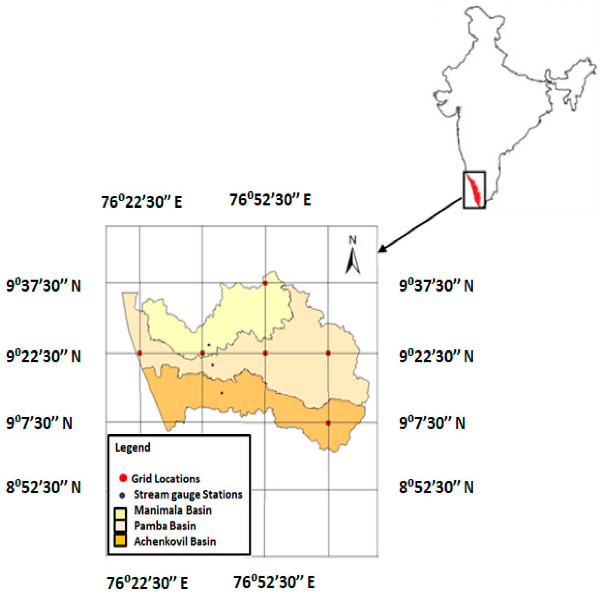
2.1. Study Area
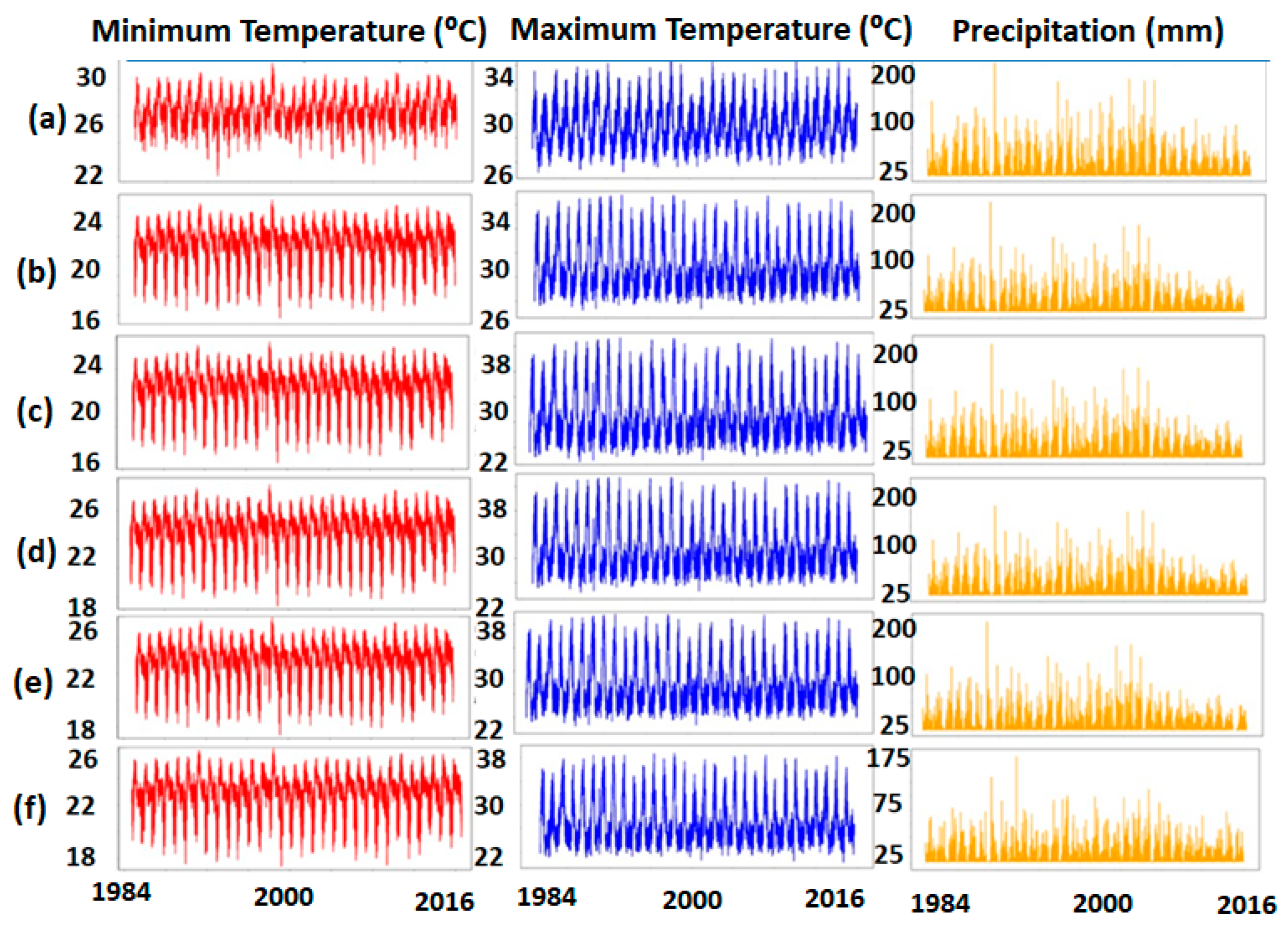
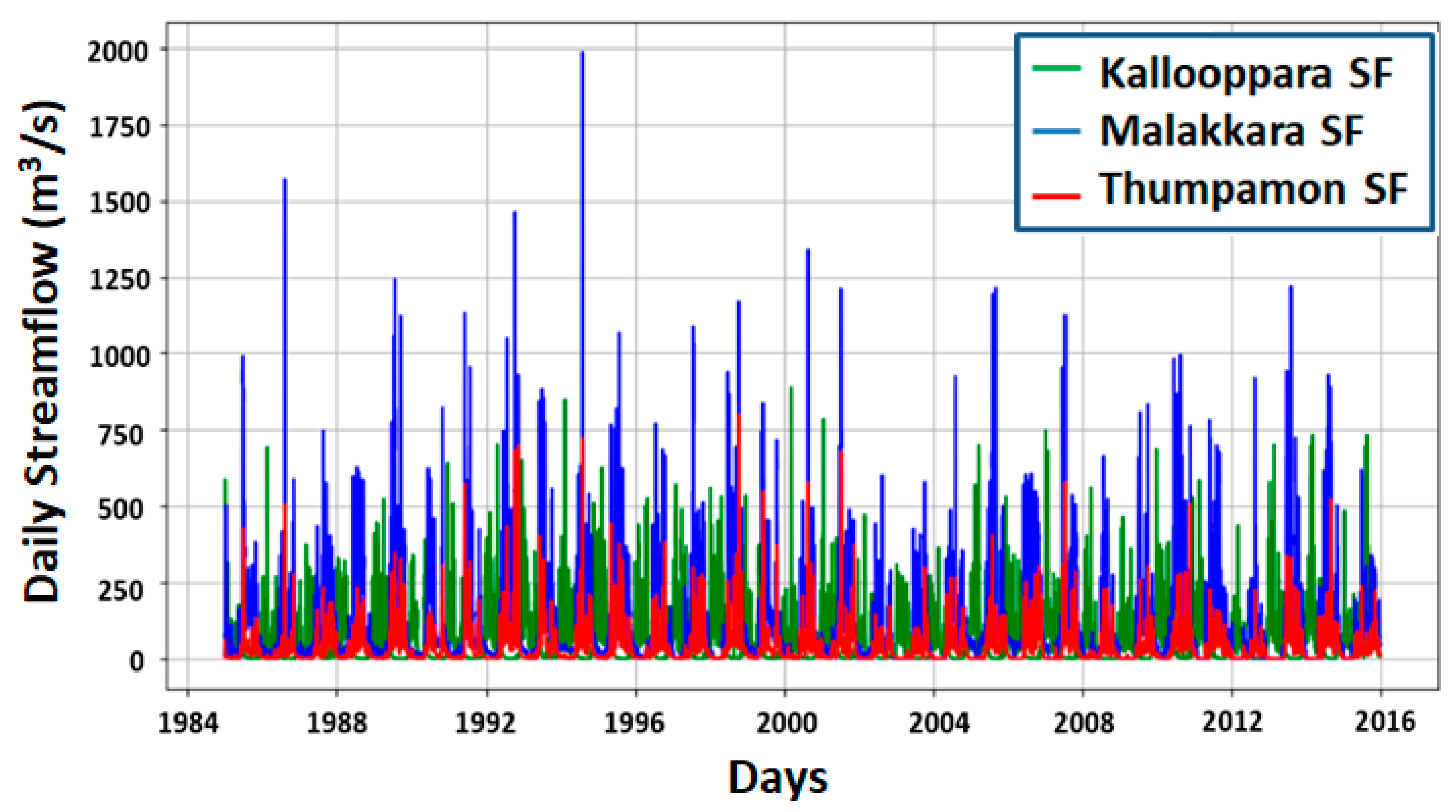
2.2. Data Sources
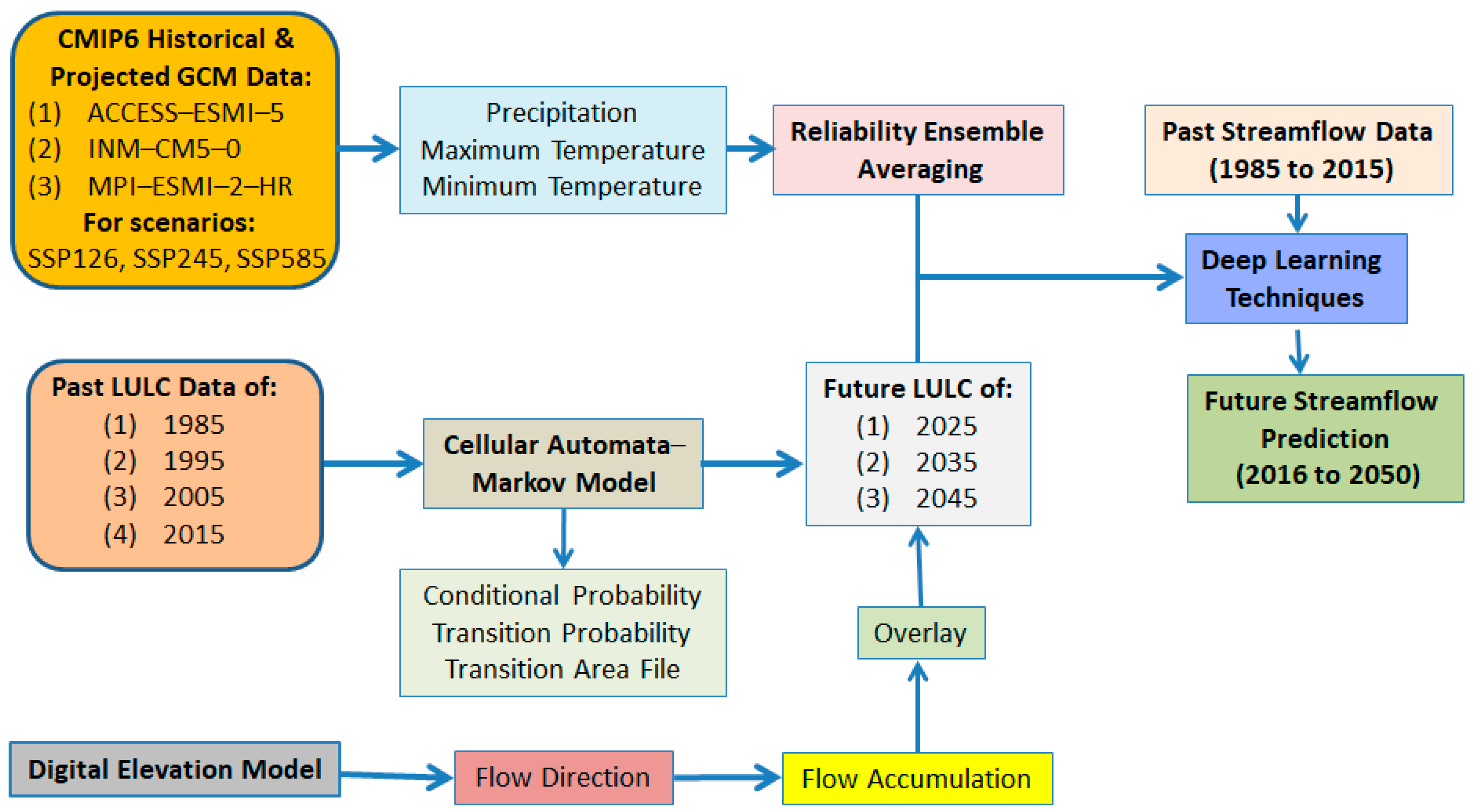
2.3. Methodology
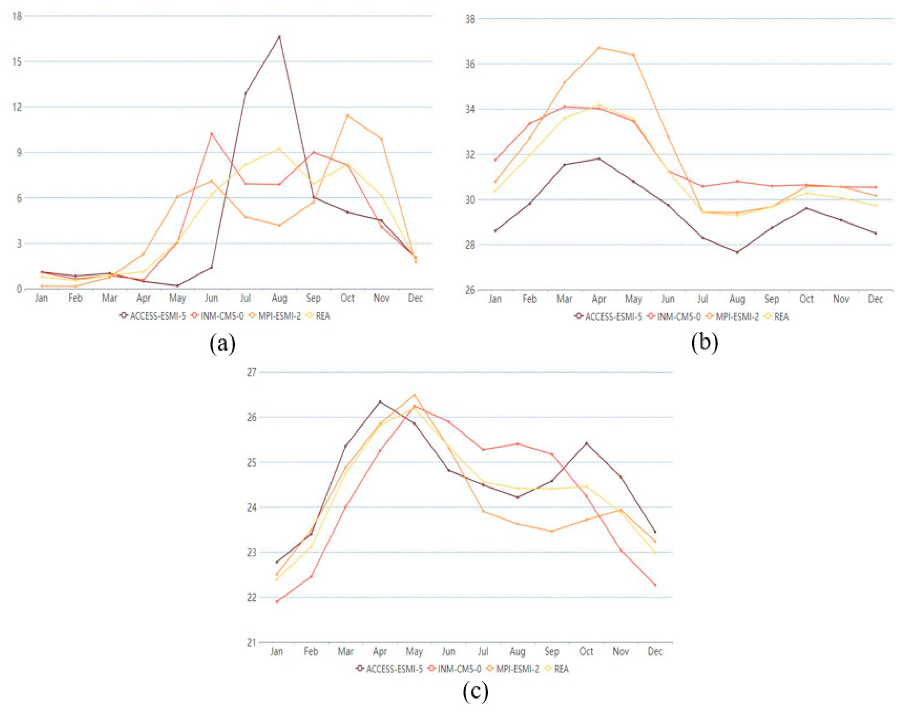
2.3.1. Reliability Ensemble Averaging
2.3.2. LULC Projection by Cellular Automata (CA)–Markov Model
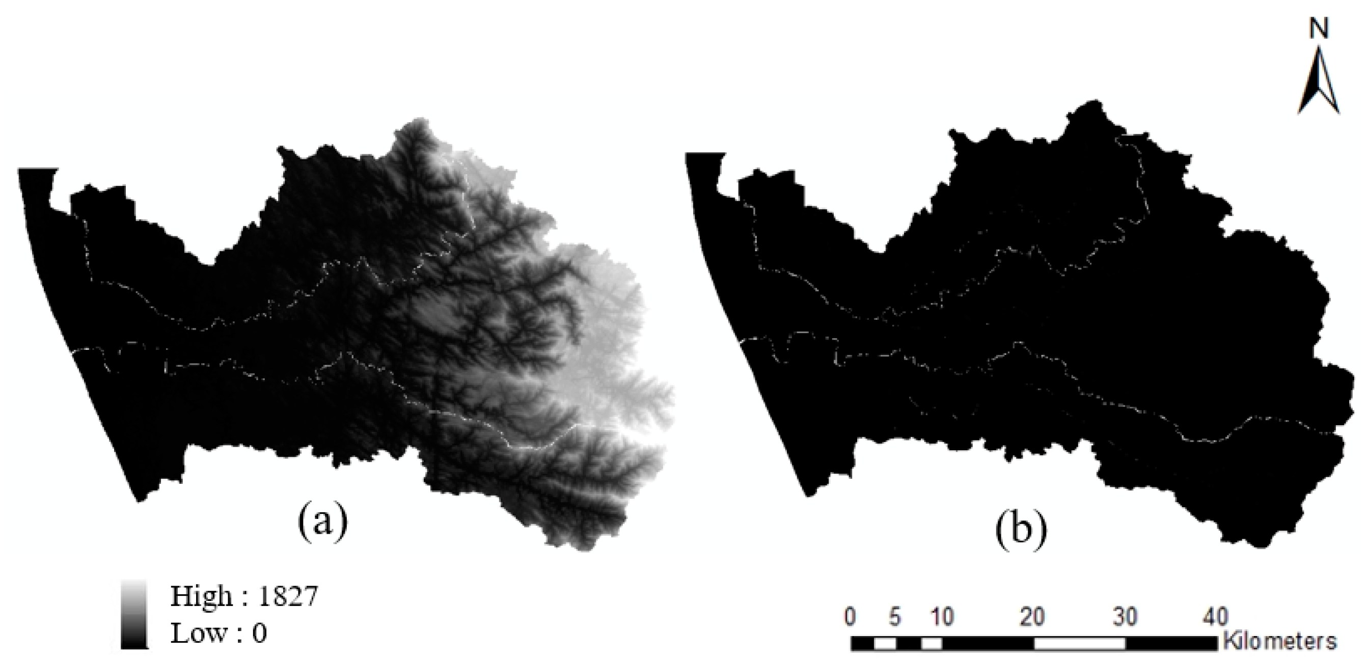
2.3.3. Flow Accumulation–LULC (FA-LULC) Overlay
2.3.4. LSTM for Future Streamflow Projection
3. Results
3.1. Reliability Ensemble Averaging for Multi-GCM Simulations
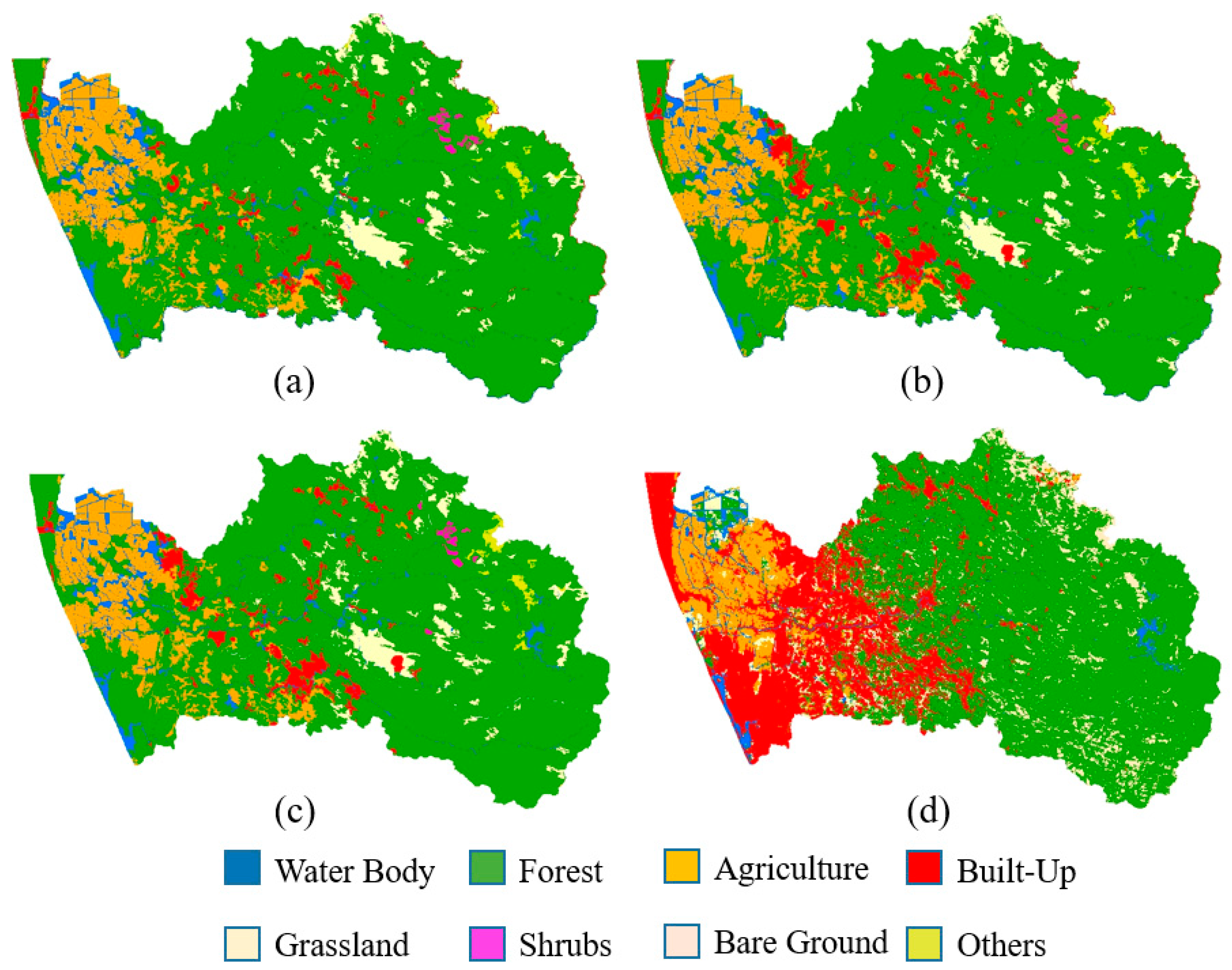
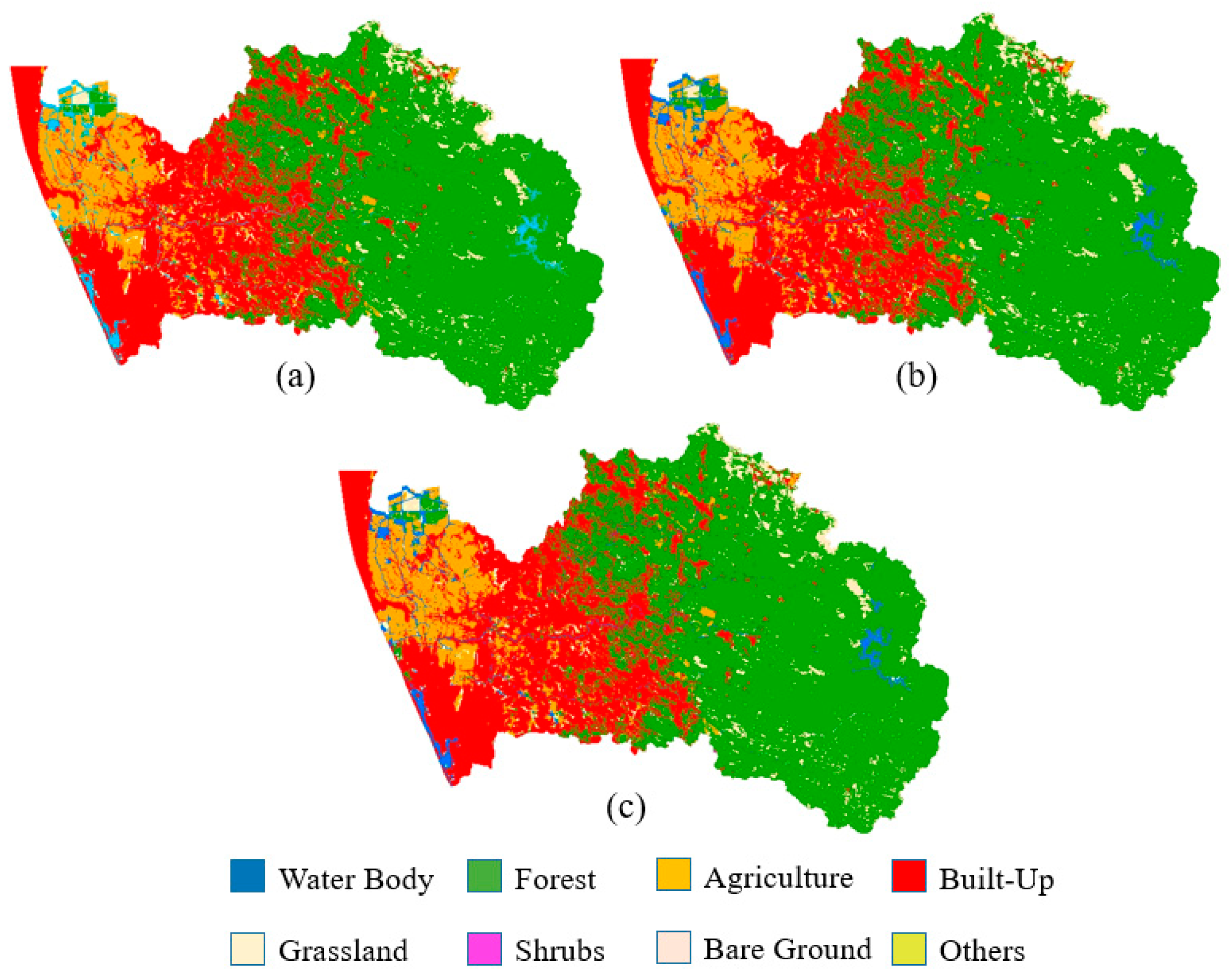
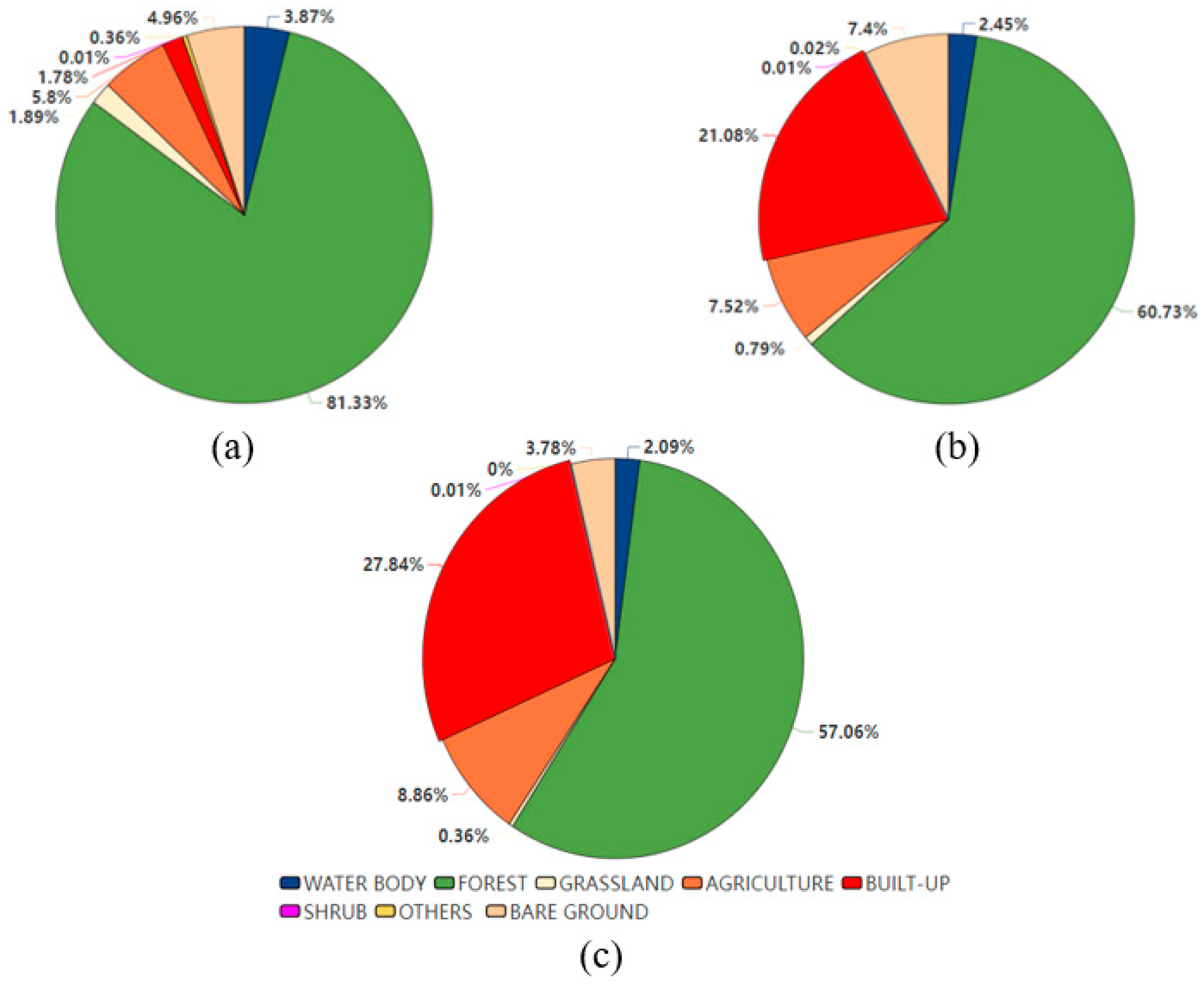
3.2. Future LULC Projection Using CA-Markov Model–MOLUSCE Plugin
- Overall Accuracy = (Sum of correctly classified pixels/Total no: of pixels) = 0.995
- Producer’s Accuracy = (User’s accuracy for actual class ‘Water Body’) = 0.968
- Precision = True Positive/(True Positive + False Positive) for ‘Water Body’= 0.98
- Recall = True Positive/(True Positive + False Negative) for ‘Water Body’ = 0.968
- F1 Score = 2×(Precision × Recall)/(Precision + Recall) for ‘Water Body’ = 0.974
3.3. Flow Accumulation-LULC Overlay Using Zonal Statistics
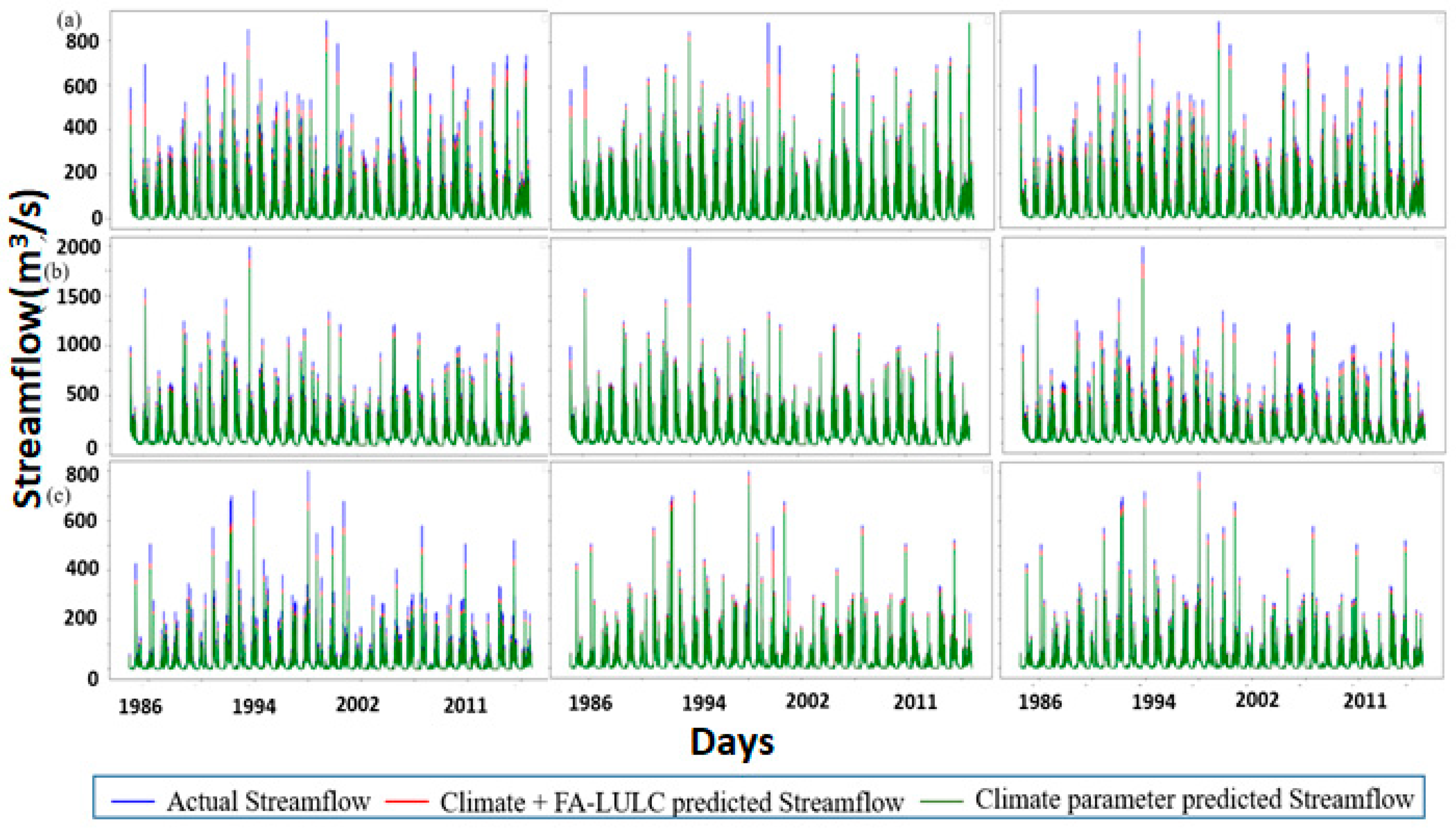
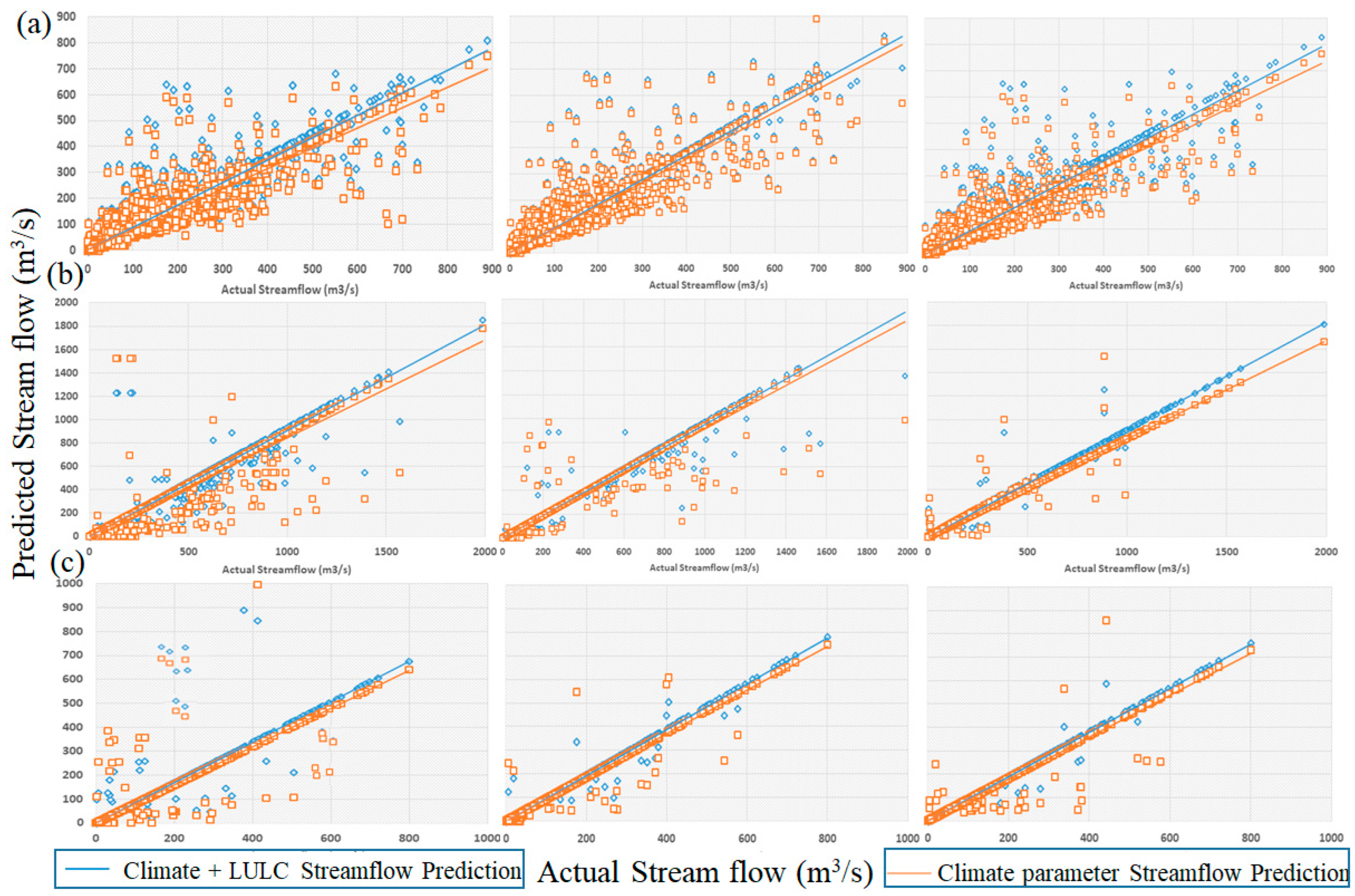
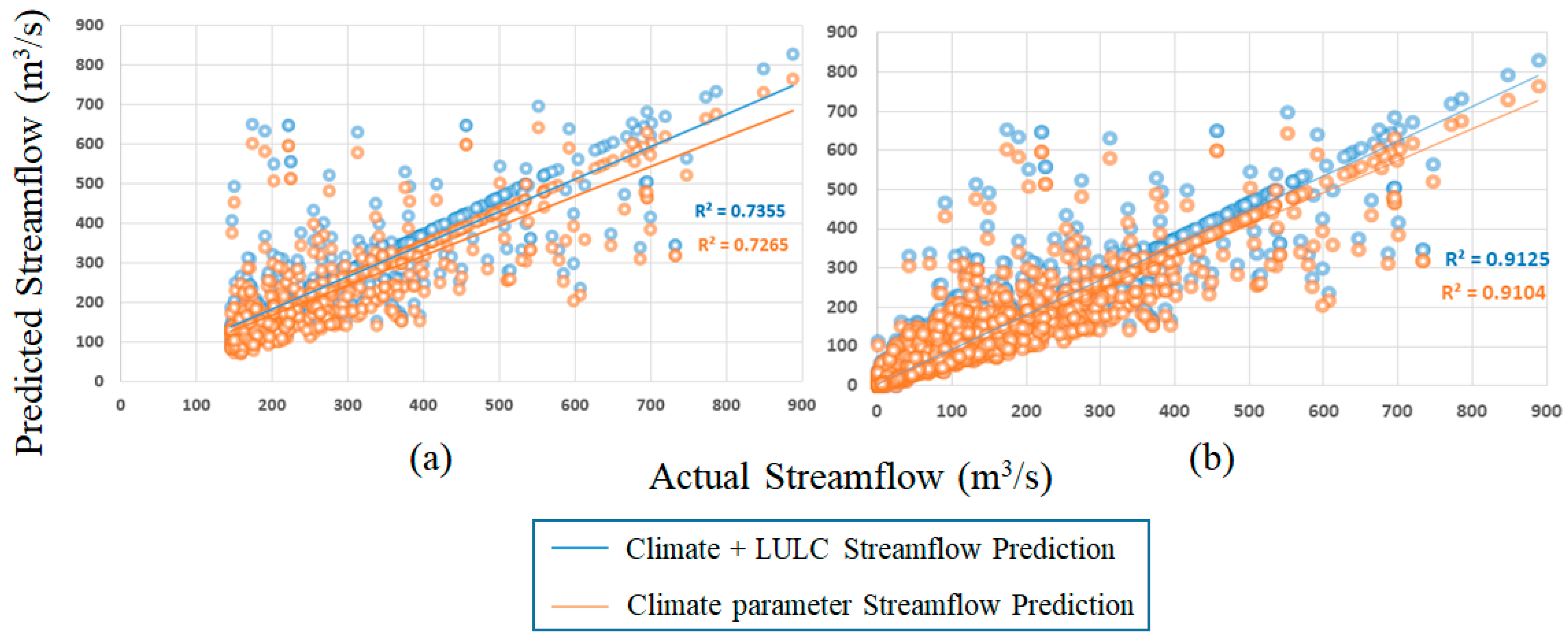
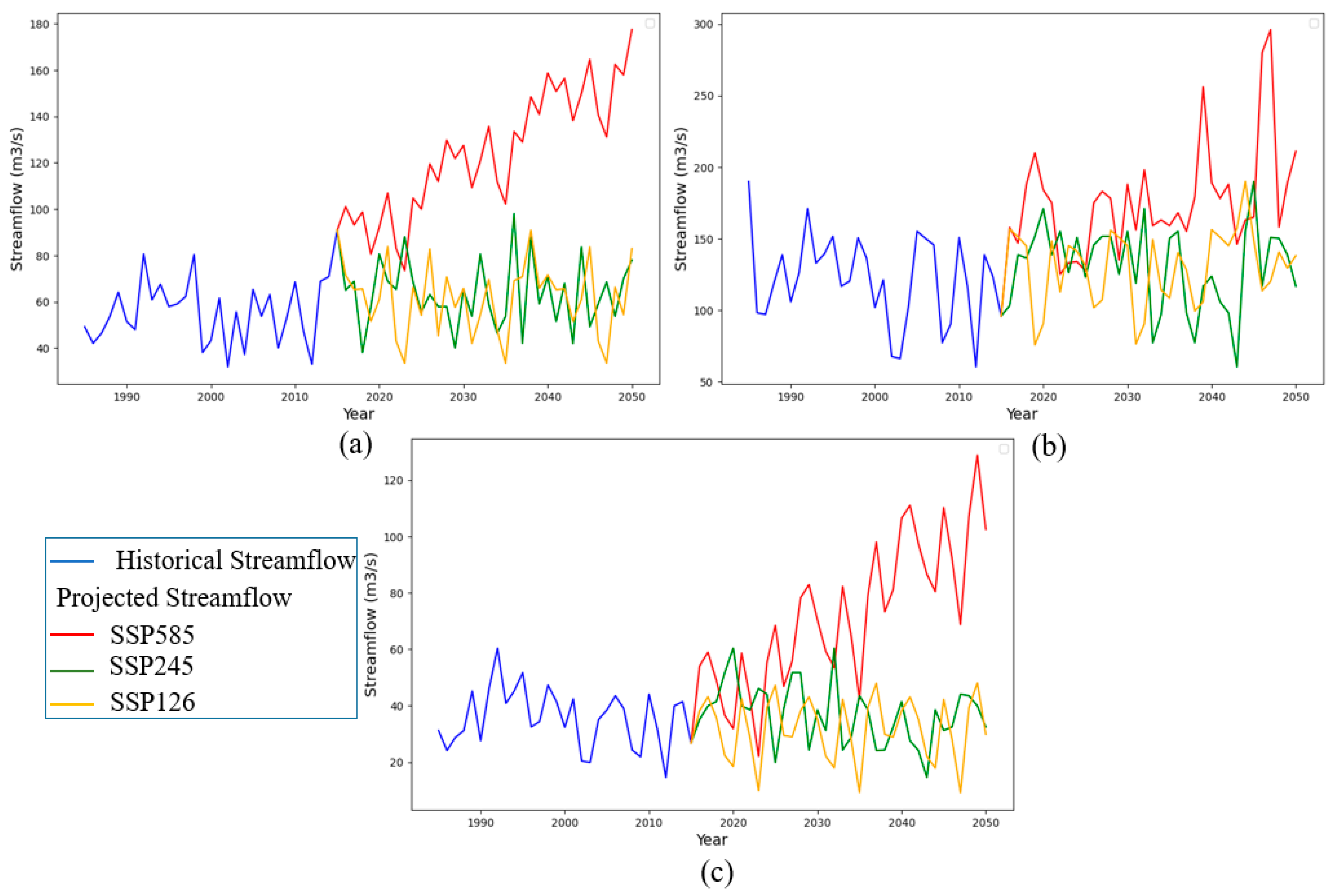
3.4. Regional-Wise Future Streamflow Projection Using LSTM
4. Comparative Analysis with Prior Studies
- In the present study, three distinct bias-corrected General Circulation Models (GCMs) outputs were combined initially using a reliability ensemble averaging approach. This method not only reduced model-specific uncertainty but also increased the precision of precipitation and temperature estimates to 2050. This is a significant improvement over earlier research that frequently depended on a single GCM output [51,52], perhaps producing forecasts that were less reliable.
- Furthermore, using the Cellular Automata (CA)-Markov model to estimate future changes in land use and land cover (LULC) gave the analysis a geographical component. This technique recognized the crucial role of future land use changes in determining streamflow patterns. This differs from many past research, which mainly concentrated on meteorological variables without specifically taking the impact of changing landscapes into account [53,54]. Conventional hydrologic studies that employ hydrologic modelling software often focus on evaluating historical LULC data to forecast future streamflow [55]. However, these studies frequently encounter a drop in accuracy as they do not account for potential changes in the landscape that may occur in the future.
- The integration of LULC data with flow accumulation (FA) can enhance the accuracy of streamflow prediction models in depicting the spatial distribution of water movement and flow channels within a watershed. FA incorporates topographic characteristics and drainage patterns, while LULC data provides insights into the types and attributes of land cover. In contrast to prior research that primarily addressed climate-driven factors [53,54,55], this approach acknowledges the complex interplay between alterations in land use and hydrological responses.
- In the context of this work, the application of deep learning methodologies for the purpose of streamflow forecasts presents a significant benefit when compared to traditional hydrologic modelling software. The use of deep learning (DL), specifically through the implementation of Long Short-Term Memory (LSTM) networks, allows our model to effectively capture complex and non-linear connections that are inherent in hydrological processes. This is in contrast to conventional hydrologic modelling methods, which frequently need manual calibration and may encounter difficulties in adequately capturing intricate dynamics [55,56]. Deep learning models has the potential to independently acquire patterns from extensive datasets, hence enhancing their forecast accuracy and capacity to adjust to dynamic circumstances. On the contrary hand, conventional hydrologic models need substantial parameter calibration [56,57]. Hydrologic models provide beneficial insights; however, the data-driven method of deep learning allows for more flexible and data-intensive studies. This technique can reveal minor variations in streamflow dynamics, resulting in more accurate forecasts in the presence of altering hydrological circumstances.
5. Conclusions
Author Contributions
Funding
Institutional Review Board Statement
Informed Consent Statement
Data Availability Statement
Acknowledgments
Conflicts of Interest
References
- Babur, S.; Gowda, R. Streamflow Response to Land-Use Land Cover change over the Nethravathi River Basin, India. J. Hydrol. Eng. 2015, 20, 05015002. [Google Scholar] [CrossRef]
- Chen, M.; Vernon, C.R.; Graham, N.T.; Hejazi, M.; Huang, M.; Cheng, Y.; Calvin, K. Global land use for 2015–2100 at 0.05° resolution under diverse socioeconomic and climate scenarios. Sci. Data 2020, 7, 320. [Google Scholar] [CrossRef] [PubMed]
- Sadhwani, K.; Eldho, T.I.; Jha, M.K.; Karmakar, S. Effects of Dynamic Land Use/Land Cover Change on Flow and Sediment Yield in a Monsoon-Dominated Tropical Watershed. Water 2022, 14, 3666. [Google Scholar] [CrossRef]
- Nourani, V.; Roushangar, K.; Andalib, G. An inverse method for watershed change detection using hybrid conceptual and artificial intelligence approaches. J. Hydrol. 2018, 562, 371–384. [Google Scholar] [CrossRef]
- Bock, L.; Lauer, A.; Schlund, M.; Barreiro, M.; Bellouin, N.; Jones, C.; Meehl, G.A.; Predoi, V.; Roberts, M.J.; Eyring, V. Quantifying Progress Across Different CMIP Phases With the ESMValTool. J. Geophys. Res. Atmos. 2020, 125, e2019JD032321. [Google Scholar] [CrossRef]
- Halmy, M.W.A.; Gessler, P.E.; Hicke, J.A.; Salem, B.B. Land use/land cover change detection and prediction in the north-western coastal desert of Egypt using Markov-CA. Appl. Geogr. 2015, 63, 101–112. [Google Scholar] [CrossRef]
- Zhang, Z.; Gao, J.; Gao, Y. The influences of land use changes on the value of ecosystem services in Chaohu Lake Basin, China. Environ. Earth Sci. 2015, 74, 385–395. [Google Scholar] [CrossRef]
- Abba Umar, D.; Ramli, M.F.; Tukur, A.I.; Jamil, N.R.; Zaudi, M.A. Detection and prediction of land use change impact on the streamflow regime in Sahelian river basin, northwestern Nigeria. H2Open J. 2021, 4, 92–113. [Google Scholar] [CrossRef]
- Mekonnen, Y.A.; Manderso, T.M. Land use/land cover change impact on streamflow using Arc-SWAT model, in case of Fetam watershed, Abbay Basin, Ethiopia. Appl. Water Sci. 2023, 13, 111. [Google Scholar] [CrossRef]
- Hyandye, C.; Martz, L.W. A Markovian and cellular automata land-use change predictive model of the Usangu Catchment. Int. J. Remote Sens. 2017, 38, 64–81. [Google Scholar] [CrossRef]
- Hamad, R.; Balzter, H.; Kolo, K. Predicting Land Use/Land Cover Changes Using a CA-Markov Model under Two Different Scenarios. Sustainability 2018, 10, 3421. [Google Scholar] [CrossRef]
- López-Vicente, M.; Pérez-Bielsa, C.; López-Montero, T.; Lambán, L.; Navas, A. Runoff simulation with eight different flow accumulation algorithms: Recommendations using a spatially distributed and open-source model. Environ. Model. Softw. 2014, 62, 11–21. [Google Scholar] [CrossRef]
- Ficklin, D.L.; Stewart, I.T.; Maurer, E.P. Climate Change Impacts on Streamflow and Subbasin-Scale Hydrology in the Upper Colorado River Basin. PLoS ONE 2013, 8, e71297. [Google Scholar] [CrossRef] [PubMed]
- Dallison, R.J.H.; Williams, A.P.; Harris, I.M.; Patil, S.D. Modelling the impact of future climate change on streamflow and water quality in Wales, UK. Hydrol. Sci. J. 2022, 67, 939–962. [Google Scholar] [CrossRef]
- Mahmoodi, N.; Kiesel, J.; Wagner, P.D.; Fohrer, N. Spatially distributed impacts of climate change and groundwater demand on the water resources in a wadi system. Hydrol. Earth Syst. Sci. 2021, 25, 5065–5081. [Google Scholar] [CrossRef]
- Parajuli, P.B.; Risal, A. Evaluation of Climate Change on Streamflow, Sediment, and Nutrient Load at Watershed Scale. Climate 2021, 9, 165. [Google Scholar] [CrossRef]
- Ismail, H.; Rowshon, M.K.; Hin, L.S.; Abdullah, A.F.B.; Nasidi, N.M. Assessment of climate change impact on future streamflow at Bernam river basin Malaysia. IOP Conf. Ser. Earth Environ. Sci. 2020, 540, 012040. [Google Scholar] [CrossRef]
- Ismail, M.; Ahmed, E.; Peng, G.; Xu, R.; Sultan, M.; Khan, F.U.; Aleem, M. Evaluating the Impact of Climate Change on the Stream Flow in Soan River Basin (Pakistan). Water 2022, 14, 3695. [Google Scholar] [CrossRef]
- Held, I.M.; Soden, B.J. Robust Responses of the Hydrological Cycle to Global Warming. J. Clim. 2006, 19, 5686–5699. [Google Scholar] [CrossRef]
- Marvel, K.; Bonfils, C. Identifying external influences on global precipitation. Proc. Natl. Acad. Sci. USA 2013, 110, 19301–19306. [Google Scholar] [CrossRef]
- Gosling, S.N.; Arnell, N.W. A global assessment of the impact of climate change on water scarcity. Clim. Chang. 2016, 134, 371–385. [Google Scholar] [CrossRef]
- Shahi, S.; Abermann, J.; Heinrich, G.; Prinz, R.; Schöner, W. Regional Variability and Trends of Temperature Inversions in Greenland. J. Clim. 2020, 33, 9391–9407. [Google Scholar] [CrossRef]
- Her, Y.; Yoo, S.H.; Cho, J.; Hwang, S.; Jeong, J.; Seong, C. Uncertainty in hydrological analysis of climate change: Multi-parameter vs. multi-GCM ensemble predictions. Sci. Rep. 2019, 9, 4974. [Google Scholar] [CrossRef] [PubMed]
- Gonzalez, P.; Neilson, R.P.; Lenihan, J.M.; Drapek, R.J. Global patterns in the vulnerability of ecosystems to vegetation shifts due to climate change. Glob. Ecol. Biogeogr. 2010, 19, 755–768. [Google Scholar] [CrossRef]
- Nourani, V.; Jabbarian Paknezhad, N.; Sharghi, E.; Khosravi, A. Estimation of prediction interval in ANN-based multi-GCMs downscaling of hydro-climatologic parameters. J. Hydrol. 2019, 579, 124226. [Google Scholar] [CrossRef]
- Baghanam, A.H.; Nourani, V.; Keynejad, M.A.; Taghipour, H.; Alami, M.T. Conjunction of wavelet-entropy and SOM clustering for multi-GCM statistical downscaling. Hydrol. Res. 2018, 50, 1–23. [Google Scholar] [CrossRef]
- Ahmed, K.; Sachindra, D.A.; Shahid, S.; Demirel, M.C.; Chung, E.S. Selection of multi-model ensemble of general circulation models for the simulation of precipitation and maximum and minimum temperature based on spatial assessment metrics. Hydrol. Earth Syst. Sci. 2019, 23, 4803–4824. [Google Scholar] [CrossRef]
- Tegegne, G.; Kim, Y.; Lee, J. Spatiotemporal Reliability Ensemble Averaging of Multimodel Simulations. Geophys. Res. Lett. 2019, 46, 12321–12330. [Google Scholar] [CrossRef]
- Cho, K.; Kim, Y. Improving streamflow prediction in the WRF-Hydro model with LSTM networks. J. Hydrol. 2022, 605, 127297. [Google Scholar] [CrossRef]
- Kumaran, N.K.P.; Padmalal, D.; Limaye, R.B.; Jennerjahn, T.; Gamre, P.G. Tropical Peat and Peatland Development in the Floodplains of the Greater Pamba Basin, South-Western India during the Holocene. PLoS ONE 2016, 11, e0154297. [Google Scholar] [CrossRef]
- Mishra, V.; Bhatia, U.; Tiwari, A.D. Bias-corrected climate projections for South Asia from Coupled Model Intercomparison Project-6. Sci. Data 2020, 7, 338. [Google Scholar] [CrossRef] [PubMed]
- Tan, Y.; Guzman, S.M.; Dong, Z.; Tan, L. Selection of Effective GCM Bias Correction Methods and Evaluation of Hydrological Response under Future Climate Scenarios. Climate 2020, 8, 108. [Google Scholar] [CrossRef]
- Hengade, N.; Eldho, T.I. Assessment of LULC and climate change on the hydrology of Ashti Catchment, India using VIC model. J. Earth Syst. Sci. 2016, 125, 1623–1634. [Google Scholar] [CrossRef]
- Gashaw, T.; Tulu, T.; Argaw, M.; Worqlul, A.W.; Tolessa, T.; Kindu, M. Estimating the impacts of land use/land cover changes on Ecosystem Service Values: The case of the Andassa watershed in the Upper Blue Nile basin of Ethiopia. Ecosyst. Serv. 2018, 31, 219–228. [Google Scholar] [CrossRef]
- Hunt, K.M.R.; Matthews, G.R.; Pappenberger, F.; Prudhomme, C. Using a long short-term memory (LSTM) neural network to boost river streamflow forecasts over the western United States. Hydrol. Earth Syst. Sci. 2022, 26, 5449–5472. [Google Scholar] [CrossRef]
- Arsenault, R.; Martel, J.L.; Brunet, F.; Brissette, F.; Mai, J. Continuous streamflow prediction in ungauged basins: Long short-term memory neural networks clearly outperform traditional hydrological models. Hydrol. Earth Syst. Sci. 2023, 27, 139–157. [Google Scholar] [CrossRef]
- Wilbrand, K.; Taormina, R.; ten Veldhuis, M.C.; Visser, M.; Hrachowitz, M.; Nuttall, J.; Dahm, R. Predicting streamflow with LSTM networks using global datasets. Front. Water 2023, 5, 1166124. [Google Scholar] [CrossRef]
- Nifa, K.; Boudhar, A.; Ouatiki, H.; Elyoussfi, H.; Bargam, B.; Chehbouni, A. Deep Learning Approach with LSTM for Daily Streamflow Prediction in a Semi-Arid Area: A Case Study of OumEr-Rbia River Basin, Morocco. Water 2023, 15, 262. [Google Scholar] [CrossRef]
- Tebaldi, C.; Knutti, R. The use of the multi-model ensemble in probabilistic climate projections. Philos. Trans. R. Soc. A Math. Phys. Eng. Sci. 2007, 365, 2053–2075. [Google Scholar] [CrossRef]
- Karimi, H.; Jafarnezhad, J.; Khaledi, J.; Ahmadi, P. Monitoring and prediction of land use/land cover changes using CA-Markov model: A case study of Ravansar County in Iran. Arab. J. Geosci. 2018, 11, 592. [Google Scholar] [CrossRef]
- Jafarpour Ghalehteimouri, K.; Shamsoddini, A.; Mousavi, M.N.; BintiCheRos, F.; Khedmatzadeh, A. Predicting spatial and decadal of land use and land cover change using integrated cellular automata Markov chain model based scenarios (2019–2049) Zarriné-Rūd River Basin in Iran. Environ. Chall. 2022, 6, 100399. [Google Scholar] [CrossRef]
- Beroho, M.; Briak, H.; Cherif, E.K.; Boulahfa, I.; Ouallali, A.; Mrabet, R.; Kebede, F.; Bernardino, A.; Aboumaria, K. Future Scenarios of Land Use/Land Cover (LULC) Based on a CA-Markov Simulation Model: Case of a Mediterranean Watershed in Morocco. Remote Sens. 2023, 15, 1162. [Google Scholar] [CrossRef]
- Mondal, M.S.; Sharma, N.; Garg, P.; Kappas, M. Statistical independence test and validation of CA Markov land use land cover (LULC) prediction results. Egypt. J. Remote Sens. Space Sci. 2016, 19, 259–272. [Google Scholar] [CrossRef]
- Hakim, A.M.Y.; Baja, S.; Rampisela, D.A.; Arif, S. Spatial dynamic prediction of landuse/landcover change (case study: Tamalanrea sub-district, makassar city). IOP Conf. Ser. Earth Environ. Sci. 2019, 280, 012023. [Google Scholar] [CrossRef]
- Abbas, Z.; Yang, G.; Zhong, Y.; Zhao, Y. Spatiotemporal Change Analysis and Future Scenario of LULC Using the CA-ANN Approach: A Case Study of the Greater Bay Area, China. Land 2021, 10, 584. [Google Scholar] [CrossRef]
- Alshari, E.A.; Gawali, B.W. Modeling Land Use Change in Sana’a City of Yemen with MOLUSCE. J. Sens. 2022, 2022, 7419031. [Google Scholar] [CrossRef]
- Kamaraj, M.; Rangarajan, S. Predicting the future land use and land cover changes for Bhavani basin, Tamil Nadu, India, using QGIS MOLUSCE plugin. Environ. Sci. Pollut. Res. 2021, 29, 86337–86348. [Google Scholar] [CrossRef]
- Hasan, M.M.; Mondol Nilay, M.S.; Jibon, N.H.; Rahman, R.M. LULC changes to riverine flooding: A case study on the Jamuna River, Bangladesh using the multilayer perceptron model. Results Eng. 2023, 18, 101079. [Google Scholar] [CrossRef]
- Apaydin, H.; Feizi, H.; Sattari, M.T.; Colak, M.S.; Shamshirband, S.; Chau, K.W. Comparative Analysis of Recurrent Neural Network Architectures for Reservoir Inflow Forecasting. Water 2020, 12, 1500. [Google Scholar] [CrossRef]
- Khan, M.; Khan, A.U.; Khan, J.; Khan, S.; Haleem, K.; Khan, F.A. Streamflow forecasting for the Hunza river basin using ANN, RNN, and ANFIS models. Water Pract. Technol. 2023, 18, 981–993. [Google Scholar] [CrossRef]
- Mansfield, L.A.; Nowack, P.J.; Kasoar, M.; Everitt, R.G.; Collins, W.J.; Voulgarakis, A. Predicting global patterns of long-term climate change from short-term simulations using machine learning. NPJ Clim. Atmos. Sci. 2020, 3, 44. [Google Scholar] [CrossRef]
- Ghosh, S. SVM-PGSL coupled approach for statistical downscaling to predict rainfall from GCM output. J. Geophys. Res. 2010, 115. [Google Scholar] [CrossRef]
- Patterson, N.K.; Lane, B.A.; Sandoval-Solis, S.; Persad, G.G.; Ortiz-Partida, J.P. Projected Effects of Temperature and Precipitation Variability Change on Streamflow Patterns Using a Functional Flows Approach. Earth’s Future 2022, 10, e2021EF002631. [Google Scholar] [CrossRef]
- Yang, T.; Wang, X.; Yu, Z.; Krysanova, V.; Chen, X.; Schwartz, F.W.; Sudicky, E.A. Climate change and probabilistic scenario of streamflow extremes in an alpine region. J. Geophys. Res. Atmos. 2014, 119, 8535–8551. [Google Scholar] [CrossRef]
- Sanjay Shekar, N.C.; Vinay, D.C. Performance of HEC-HMS and SWAT to simulate streamflow in the sub-humid tropical Hemavathi catchment. J. Water Clim. Chang. 2021, 12, 3005–3017. [Google Scholar] [CrossRef]
- Malik, M.A.; Dar, A.Q.; Jain, M.K. Modelling streamflow using the SWAT model and multi-site calibration utilizing SUFI-2 of SWAT-CUP model for high altitude catchments, NW Himalaya’s. Model. Earth Syst. Environ. 2022, 8, 1203–1213. [Google Scholar] [CrossRef]
- Singh, L.; Saravanan, S. Simulation of monthly streamflow using the SWAT model of the Ib River watershed, India. HydroResearch 2020, 3, 95–105. [Google Scholar] [CrossRef]


| Grid Locations | Parameters | Maxi. Value | Min. Value | Standard Deviation | Coefficient of Variation | Best Fit Distribution |
|---|---|---|---|---|---|---|
| 76.375/9.375 | Precipitation | 201.23 | 0 | 17.35 | 1.44 | GEV |
| Maximum Temperature | 31.02 | 25.11 | 0.796 | 0.03 | Normal | |
| Minimum Temperature | 28.63 | 23.74 | 0.729 | 0.02 | Gamma | |
| 76.625/9.375 | Precipitation | 201.19 | 0 | 14.75 | 1.51 | Log-Logistic |
| Maximum Temperature | 33.7 | 22.69 | 1.23 | 0.04 | Gamma | |
| Minimum Temperature | 24.5 | 18.72 | 0.722 | 0.03 | Normal | |
| 76.875/9.375 | Precipitation | 200.36 | 0 | 14.8 | 2.09 | GEV |
| Maximum Temperature | 33.7 | 23.65 | 1.23 | 0.04 | Normal | |
| Minimum Temperature | 24.67 | 21.36 | 0.62 | 0.03 | Normal | |
| 76.875/9.625 | Precipitation | 210.36 | 0 | 11.26 | 1.9 | Log-Pearson Type III |
| Maximum Temperature | 36.69 | 26.54 | 1.51 | 0.03 | Normal | |
| Minimum Temperature | 27.43 | 21.99 | 0.74 | 0.04 | Gamma | |
| 77.125/9.375 | Precipitation | 196.35 | 0 | 14.61 | 2.03 | GEV |
| Maximum Temperature | 33.56 | 24.39 | 1.96 | 0.06 | Beta | |
| Minimum Temperature | 27.96 | 21.78 | 0.64 | 0.03 | Normal | |
| 77.125/9.125 | Precipitation | 168.69 | 0 | 13.99 | 1.88 | GEV |
| Maximum Temperature | 34.35 | 26.57 | 1.51 | 0.08 | Gamma | |
| Minimum Temperature | 27.26 | 21.56 | 0.09 | 0.03 | Normal |
| Model | Activation Function | Hidden Layer 1 | Dropout | Hidden Layer 2 | Dropout | Hidden Layer 3 | Dense Layer 1 | Dense Layer 2 |
|---|---|---|---|---|---|---|---|---|
| LSTM | ReLU | LSTM 75 Units | 0.25 | 50 Units | 0.5 | 50 Units | 25 Units | 1 Unit |
| Actual Classes | Water Body | Forest | Grassland | Agriculture | Built-Up | Shrub | Bare Ground | Others |
|---|---|---|---|---|---|---|---|---|
| Predicted Water body | 1,013,222 | 12,368 | 758 | 876 | 18,888 | 78 | 0 | 101 |
| Predicted Forest | 7541 | 25,510,333 | 2563 | 958 | 16,523 | 196 | 0 | 189 |
| Predicted Grassland | 251 | 15,651 | 115,231 | 772 | 13,269 | 101 | 0 | 336 |
| Predicted Agriculture | 4470 | 14,789 | 3589 | 4,100,777 | 17,536 | 111 | 0 | 2358 |
| Predicted Built-Up | 2517 | 1369 | 523 | 638 | 11,548,354 | 0 | 0 | 63 |
| Predicted Shrub | 1888 | 7569 | 999 | 1056 | 19,638 | 4012 | 0 | 785 |
| Predicted Bare Ground | 986 | 14,500 | 478 | 987 | 11,258 | 53 | 2 | 569 |
| Predicted Others | 2288 | 5431 | 5270 | 3712 | 9175 | 110 | 0 | 2,490,030 |
| Total | 1,033,163 | 25,582,010 | 129,411 | 4,109,776 | 11,654,641 | 4661 | 2 | 2,494,431 |
| Value | Label | Count | Area (km2) | Min | Max | Range | Sum |
|---|---|---|---|---|---|---|---|
| 1 | Water Body | 298,526 | 29.8526 | 1 | 9 | 8 | 315,895 |
| 2 | Forest | 9,001,197 | 900.1197 | 1 | 9 | 8 | 9,040,508 |
| 3 | Grassland | 40,065 | 4.0065 | 1 | 3 | 2 | 40,238 |
| 4 | Agriculture | 1,183,885 | 118.3885 | 1 | 9 | 8 | 1,185,904 |
| 5 | Built-Up | 1,845,417 | 184.5417 | 1 | 9 | 8 | 1,855,177 |
| 6 | Shrub | 1584 | 0.1584 | 1 | 8 | 7 | 1640 |
| 7 | Others | 4517 | 0.4517 | 1 | 2 | 1 | 4518 |
| 8 | Bare Ground | 937,272 | 93.7272 | 1 | 7 | 6 | 939,986 |
| Performance Evaluators | R2 | RMSE | MSE | MAE | NSE |
|---|---|---|---|---|---|
| KALLOOPPARA SSP126 | |||||
| Climate + LULC | 0.9 | 27.24 | 742.11 | 10.07 | 0.91 |
| Climate | 0.87 | 31.89 | 1017.17 | 13.12 | 0.86 |
| KALLOOPPARA SSP245 | |||||
| Climate + LULC | 0.92 | 26.31 | 692.25 | 7.63 | 0.92 |
| Climate | 0.89 | 27.47 | 754.95 | 8.79 | 0.9 |
| KALLOOPPARA SSP585 | |||||
| Climate + LULC | 0.91 | 26.62 | 708.71 | 9.16 | 0.92 |
| Climate | 0.88 | 29.08 | 846.15 | 12.09 | 0.89 |
| MALAKKARA SSP126 | |||||
| Climate + LULC | 0.99 | 13.58 | 184.68 | 8.07 | 0.97 |
| Climate | 0.95 | 21.33 | 454.97 | 12.68 | 0.99 |
| MALAKKARA SSP245 | |||||
| Climate + LULC | 0.99 | 5.12 | 26.17 | 3.04 | 0.97 |
| Climate | 0.95 | 10.37 | 107.49 | 6.16 | 0.94 |
| MALAKKARA SSP585 | |||||
| Climate + LULC | 0.98 | 17.97 | 323.02 | 10.68 | 0.97 |
| Climate | 0.94 | 33.01 | 1089.09 | 19.62 | 0.95 |
| THUMPAMON SSP126 | |||||
| Climate + LULC | 0.97 | 10.97 | 120.36 | 5.61 | 0.96 |
| Climate | 0.92 | 13.94 | 194.37 | 7.13 | 0.9 |
| THUMPAMON SSP245 | |||||
| Climate + LULC | 0.99 | 1.76 | 3.11 | 0.91 | 0.98 |
| Climate | 0.91 | 4.68 | 21.98 | 2.34 | 0.91 |
| THUMPAMON SSP585 | |||||
| Climate + LULC | 0.99 | 3.58 | 12.79 | 1.83 | 0.98 |
| Climate | 0.97 | 6.21 | 38.45 | 3.17 | 0.96 |
Disclaimer/Publisher’s Note: The statements, opinions and data contained in all publications are solely those of the individual author(s) and contributor(s) and not of MDPI and/or the editor(s). MDPI and/or the editor(s) disclaim responsibility for any injury to people or property resulting from any ideas, methods, instructions or products referred to in the content. |
© 2023 by the authors. Licensee MDPI, Basel, Switzerland. This article is an open access article distributed under the terms and conditions of the Creative Commons Attribution (CC BY) license (https://creativecommons.org/licenses/by/4.0/).
Share and Cite
Geetha Raveendran Nair, A.N.; Shamsudeen, S.D.; Mohan, M.G.; Sankaran, A. Basin-Scale Streamflow Projections for Greater Pamba River Basin, India Integrating GCM Ensemble Modelling and Flow Accumulation-Weighted LULC Overlay in Deep Learning Environment. Sustainability 2023, 15, 14148. https://doi.org/10.3390/su151914148
Geetha Raveendran Nair AN, Shamsudeen SD, Mohan MG, Sankaran A. Basin-Scale Streamflow Projections for Greater Pamba River Basin, India Integrating GCM Ensemble Modelling and Flow Accumulation-Weighted LULC Overlay in Deep Learning Environment. Sustainability. 2023; 15(19):14148. https://doi.org/10.3390/su151914148
Chicago/Turabian StyleGeetha Raveendran Nair, Arathy Nair, Shamla Dilama Shamsudeen, Meera Geetha Mohan, and Adarsh Sankaran. 2023. "Basin-Scale Streamflow Projections for Greater Pamba River Basin, India Integrating GCM Ensemble Modelling and Flow Accumulation-Weighted LULC Overlay in Deep Learning Environment" Sustainability 15, no. 19: 14148. https://doi.org/10.3390/su151914148