


A New Distribution for Modeling Data with Increasing Hazard Rate: A Case of COVID-19 Pandemic and Vinyl Chloride Data

 , , , , and
Abstract
:1. Introduction
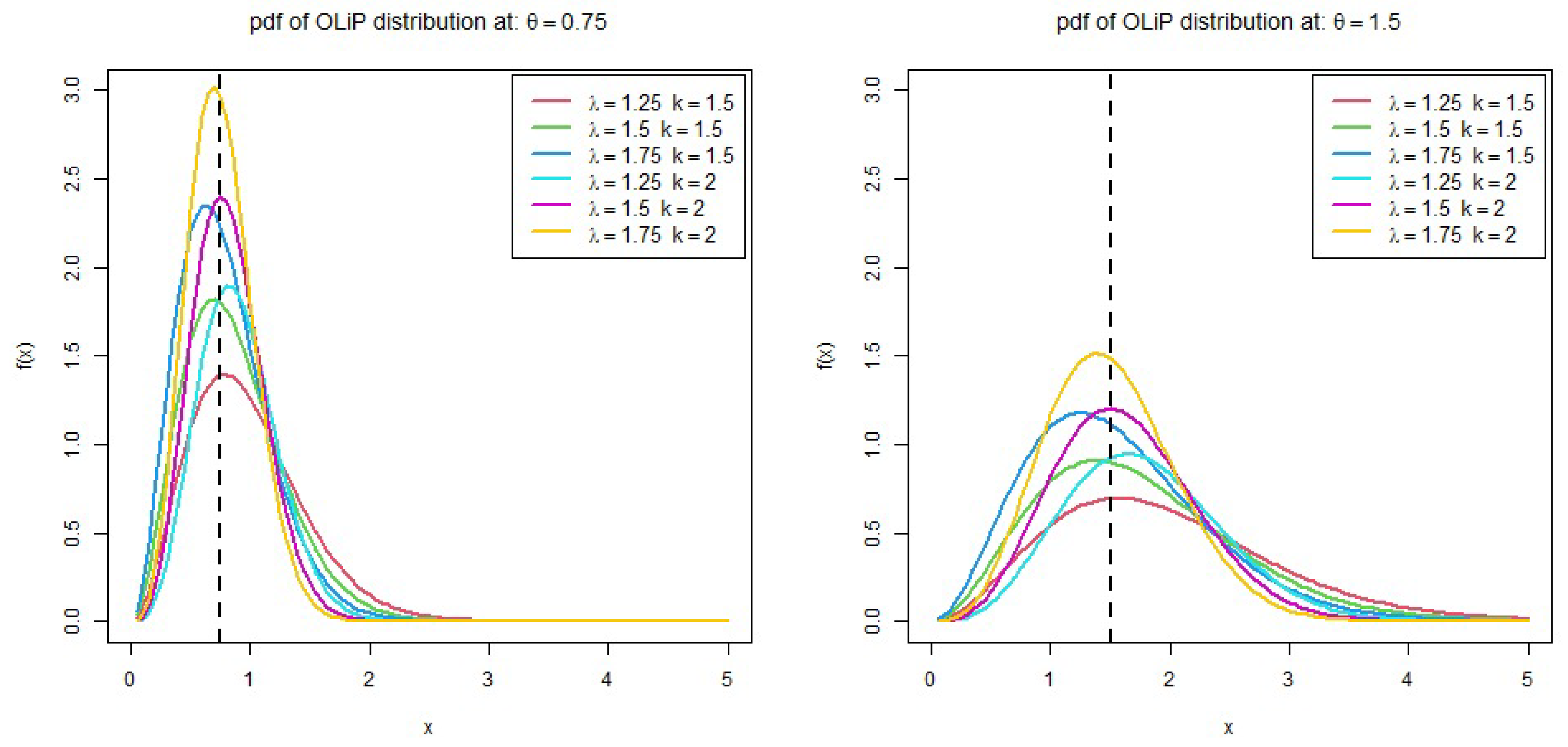
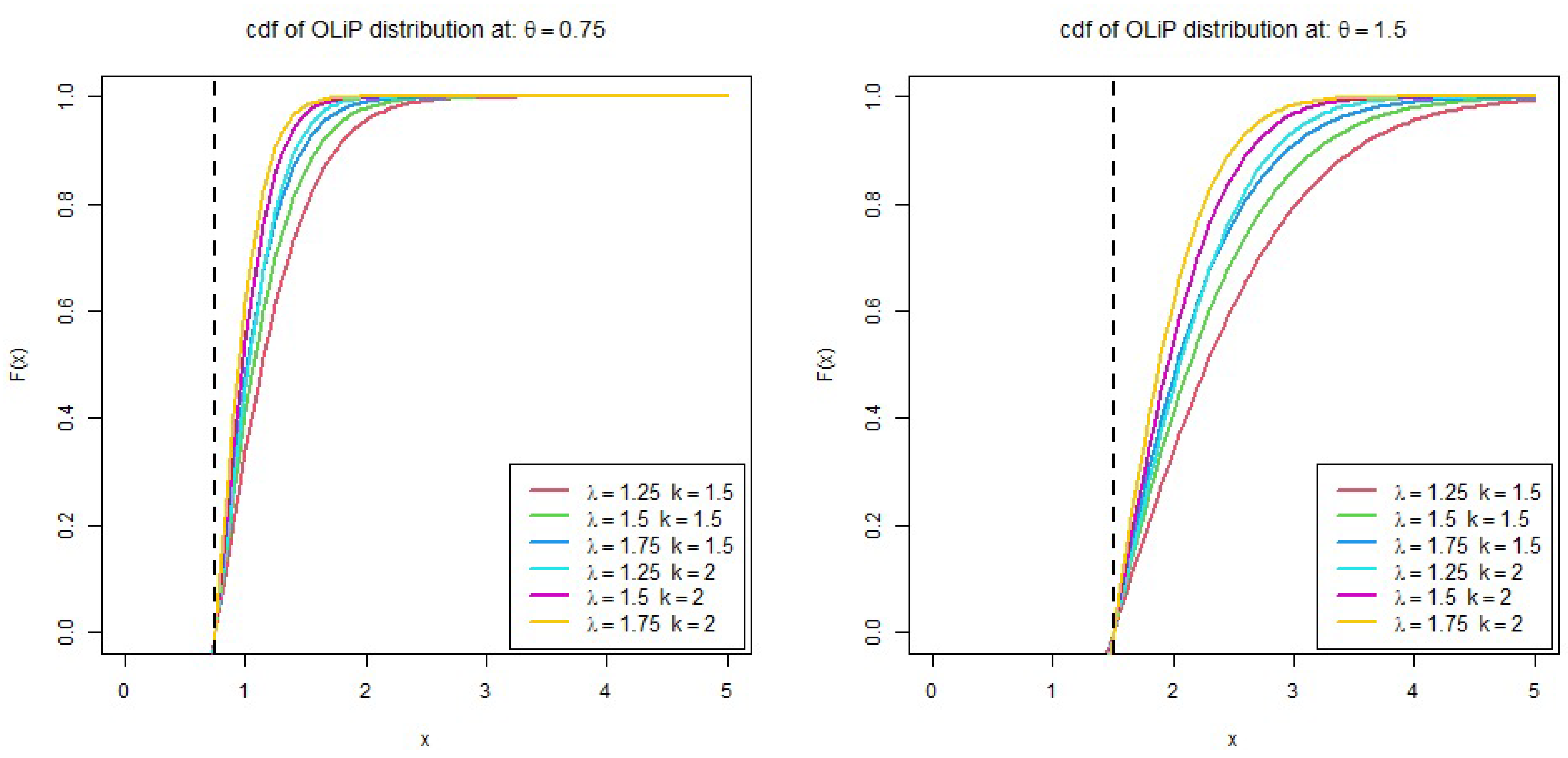
2. The New Distribution
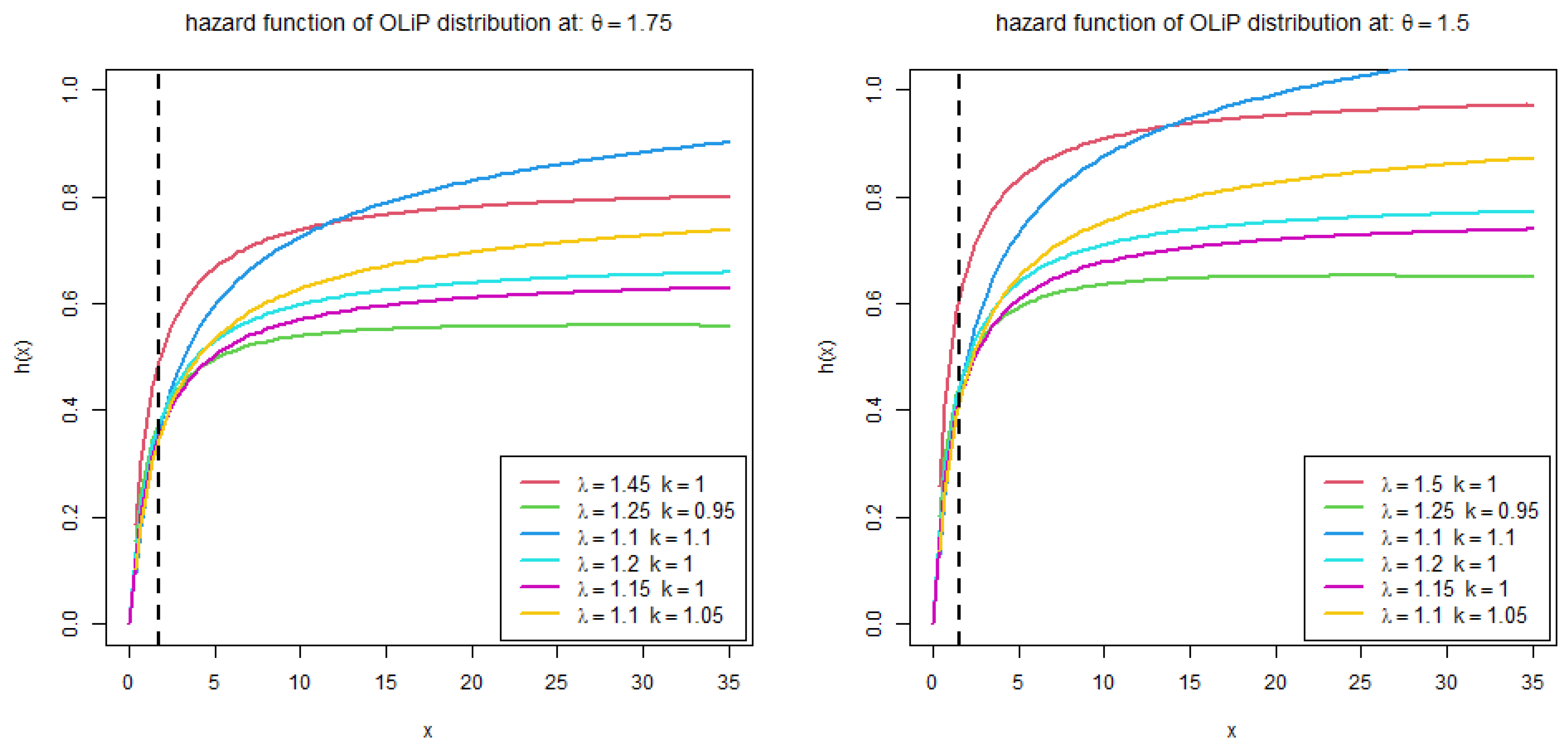
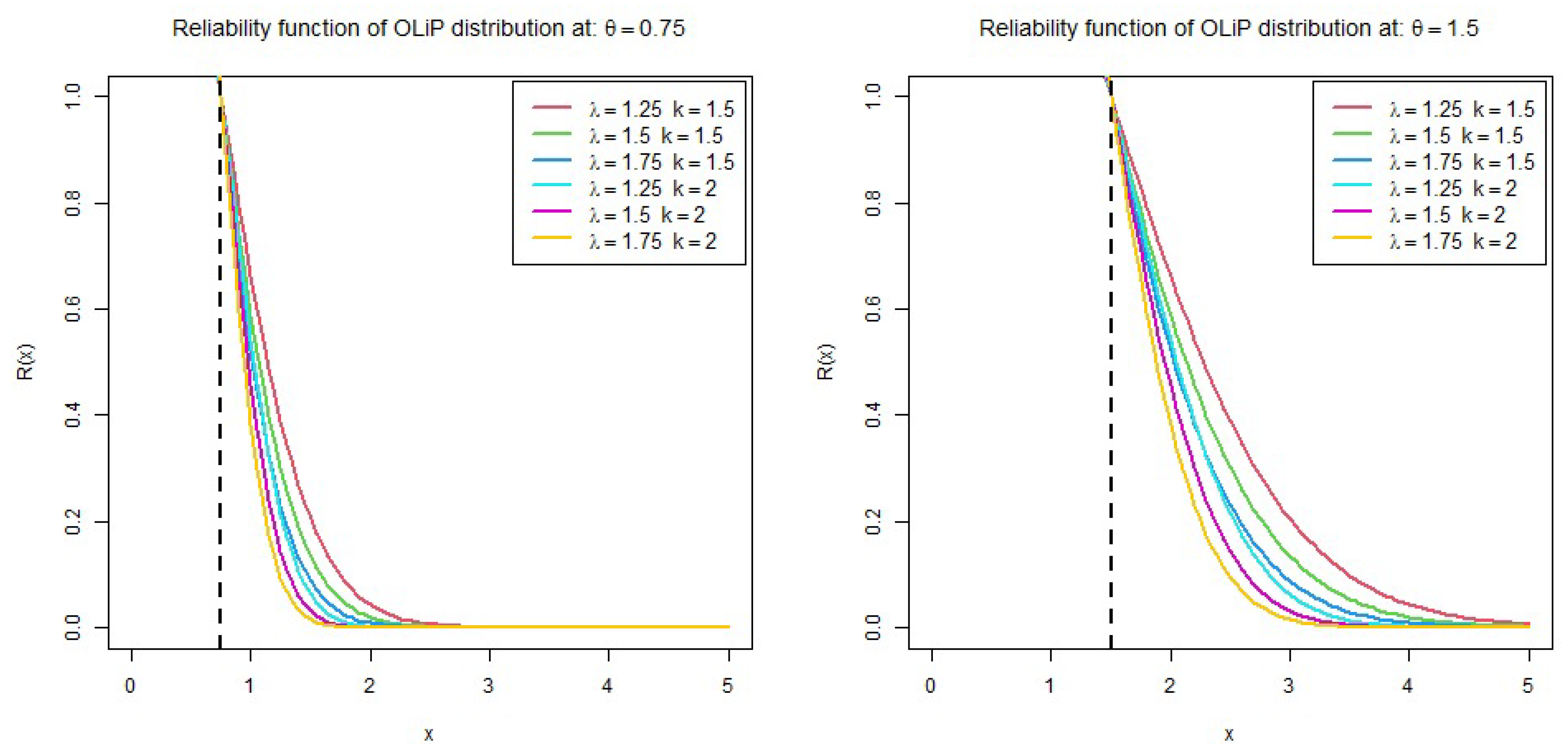
3. Statistical Properties of OLiP Distribution
3.1. The OLiP Distribution’s Moment
3.2. Skewness and Kurtosis Coefficients for the OLiP Distribution
3.3. The OLiP Distribution’s Moment-Generating and Characteristic Functions
3.4. Order Statistics of the OLiP Distribution
3.5. Entropy and Asymptotic Behavior of the OLiP Distribution
3.6. Stochastic Ordering of OLiP Distribution
- (i)
- Stochastic order if .
- (ii)
- Hazard rate order if .
- (iii)
- Mean residual life order if .
- (iv)
- Likelihood ratio order if decreases in x.
4. Non-Bayesian Estimation of OLiP Distribution Parameters
4.1. Maximum Likelihood Estimation (MLE)
4.2. Maximum Product Space Estimators (MPSE)
4.3. Least Squares Estimation (LSE)
4.4. Weighted Least Squares Estimation (WLSE)
4.5. Cramér–von Mises Estimation (CVME)
4.6. Anderson–Darling Estimation (ADE)
4.7. Right-Tailed Anderson–Darling Estimation (RTADE)
5. Bayesian Estimation of OLiP Distribution Parameters
6. Single Acceptance Sampling Plans
- (1)
- Take n units at random from the proposed lot as a sample.
- (2)
- Run the following test for units of time.Accept the entire lot if c or fewer units (the acceptance number) fail throughout the experiment; else, reject the entire lot.
- The consumer’s risk is given as and .
- The acceptance number c is given as and 10.
- The constant a is assumed to be and . If , thus is the median life time ).
- The parameters of the OLiP distribution are assumed as:
- With increasing and c, the required sample size n increases and decreases.
- With increasing a, the required sample size n decreases and increases.
- With increasing and fixed k, the required sample size n increases and decreases.
- With increasing k and fixed , the required sample size n increases and decreases.

| c | |||||||||||
|---|---|---|---|---|---|---|---|---|---|---|---|
| 0.3 | 0 | 1 | 1.00000 | 1 | 1.00000 | 1 | 1.00000 | 1 | 1.00000 | 1 | 1.00000 |
| 2 | 7 | 0.77621 | 6 | 0.77887 | 5 | 0.81397 | 4 | 0.89188 | 4 | 0.87500 | |
| 4 | 13 | 0.76870 | 11 | 0.77123 | 9 | 0.81711 | 8 | 0.81031 | 8 | 0.77344 | |
| 8 | 25 | 0.78632 | 21 | 0.78889 | 18 | 0.78665 | 16 | 0.75800 | 15 | 0.78802 | |
| 10 | 32 | 0.76146 | 27 | 0.75451 | 23 | 0.75429 | 19 | 0.81809 | 19 | 0.75966 | |
| 0.6 | 0 | 5 | 0.26519 | 4 | 0.28639 | 3 | 0.35299 | 3 | 0.27416 | 2 | 0.50000 |
| 2 | 13 | 0.29732 | 11 | 0.28186 | 9 | 0.30325 | 8 | 0.26709 | 7 | 0.34375 | |
| 4 | 22 | 0.25067 | 18 | 0.25979 | 15 | 0.26432 | 12 | 0.33005 | 12 | 0.27441 | |
| 8 | 37 | 0.27468 | 31 | 0.25731 | 26 | 0.25397 | 22 | 0.25670 | 21 | 0.25172 | |
| 10 | 45 | 0.26454 | 37 | 0.27098 | 31 | 0.26938 | 26 | 0.28741 | 25 | 0.27063 | |
| 0.95 | 0 | 10 | 0.05047 | 8 | 0.05406 | 6 | 0.07403 | 5 | 0.07517 | 5 | 0.06250 |
| 2 | 21 | 0.05022 | 17 | 0.05253 | 14 | 0.05319 | 11 | 0.07334 | 11 | 0.05469 | |
| 4 | 30 | 0.05742 | 25 | 0.05100 | 20 | 0.06303 | 17 | 0.05694 | 16 | 0.05923 | |
| 8 | 48 | 0.05605 | 39 | 0.05989 | 33 | 0.05022 | 27 | 0.06216 | 26 | 0.05388 | |
| 10 | 57 | 0.05281 | 46 | 0.06056 | 38 | 0.06282 | 32 | 0.06123 | 30 | 0.06802 | |
| 0.3 | 0 | 1 | 1.00000 | 1 | 1.00000 | 1 | 1.00000 | 1 | 1.00000 | 1 | 1.00000 |
| 2 | 7 | 0.79279 | 6 | 0.78878 | 5 | 0.81826 | 4 | 0.89246 | 4 | 0.87500 | |
| 4 | 13 | 0.79167 | 11 | 0.78502 | 9 | 0.82291 | 8 | 0.81158 | 8 | 0.77344 | |
| 8 | 26 | 0.77873 | 22 | 0.75731 | 18 | 0.79573 | 16 | 0.76010 | 15 | 0.78802 | |
| 10 | 33 | 0.76316 | 27 | 0.77690 | 23 | 0.76541 | 19 | 0.82002 | 19 | 0.75966 | |
| 0.6 | 0 | 5 | 0.27954 | 4 | 0.29509 | 3 | 0.35737 | 3 | 0.27506 | 2 | 0.50000 |
| 2 | 14 | 0.26784 | 11 | 0.29703 | 9 | 0.31082 | 8 | 0.26862 | 7 | 0.34375 | |
| 4 | 22 | 0.28229 | 18 | 0.27875 | 15 | 0.27361 | 12 | 0.33215 | 12 | 0.27441 | |
| 8 | 39 | 0.25313 | 31 | 0.28247 | 26 | 0.26611 | 22 | 0.25925 | 21 | 0.25172 | |
| 10 | 47 | 0.25310 | 38 | 0.26165 | 31 | 0.28309 | 26 | 0.29036 | 25 | 0.27063 | |
| 0.95 | 0 | 10 | 0.05682 | 8 | 0.05797 | 6 | 0.07635 | 5 | 0.07566 | 5 | 0.06250 |
| 2 | 21 | 0.06019 | 17 | 0.05851 | 14 | 0.05610 | 11 | 0.07410 | 11 | 0.05469 | |
| 4 | 31 | 0.05865 | 25 | 0.05829 | 20 | 0.06709 | 17 | 0.05772 | 16 | 0.05923 | |
| 8 | 50 | 0.05397 | 40 | 0.05778 | 33 | 0.05467 | 27 | 0.06323 | 26 | 0.05388 | |
| 10 | 59 | 0.05351 | 47 | 0.06018 | 39 | 0.05417 | 32 | 0.06239 | 30 | 0.06802 | |
| c | |||||||||||
|---|---|---|---|---|---|---|---|---|---|---|---|
| 0.3 | 0 | 2 | 0.79910 | 1 | 1.00000 | 1 | 1.00000 | 1 | 1.00000 | 1 | 1.00000 |
| 2 | 9 | 0.79493 | 7 | 0.79149 | 5 | 0.86157 | 4 | 0.89963 | 4 | 0.87500 | |
| 4 | 18 | 0.75514 | 13 | 0.78988 | 10 | 0.80705 | 8 | 0.82714 | 8 | 0.77344 | |
| 8 | 35 | 0.76897 | 26 | 0.77609 | 20 | 0.78240 | 16 | 0.78580 | 15 | 0.78802 | |
| 10 | 44 | 0.76647 | 33 | 0.76008 | 25 | 0.78077 | 20 | 0.77903 | 19 | 0.75966 | |
| 0.6 | 0 | 7 | 0.26037 | 5 | 0.27837 | 4 | 0.25946 | 3 | 0.28651 | 3 | 0.25000 |
| 2 | 19 | 0.26824 | 14 | 0.26584 | 10 | 0.30950 | 8 | 0.28839 | 7 | 0.34375 | |
| 4 | 31 | 0.25136 | 22 | 0.27968 | 17 | 0.25543 | 13 | 0.26907 | 12 | 0.27441 | |
| 8 | 53 | 0.25658 | 38 | 0.28106 | 29 | 0.26327 | 22 | 0.29266 | 21 | 0.25172 | |
| 10 | 64 | 0.25448 | 46 | 0.27784 | 35 | 0.26216 | 27 | 0.26821 | 25 | 0.27063 | |
| 0.95 | 0 | 14 | 0.05417 | 10 | 0.05629 | 7 | 0.06732 | 5 | 0.08209 | 5 | 0.06250 |
| 2 | 30 | 0.05085 | 21 | 0.05934 | 16 | 0.05100 | 12 | 0.05375 | 11 | 0.05469 | |
| 4 | 43 | 0.05643 | 31 | 0.05761 | 23 | 0.05708 | 17 | 0.06839 | 16 | 0.05923 | |
| 8 | 69 | 0.05283 | 50 | 0.05273 | 37 | 0.05411 | 28 | 0.05753 | 26 | 0.05388 | |
| 10 | 81 | 0.05430 | 59 | 0.05216 | 44 | 0.05038 | 33 | 0.05923 | 30 | 0.06802 | |
| 0.3 | 0 | 2 | 0.81308 | 1 | 1.00000 | 1 | 1.00000 | 1 | 1.00000 | 1 | 1.00000 |
| 2 | 10 | 0.77215 | 7 | 0.80838 | 6 | 0.75452 | 4 | 0.90046 | 4 | 0.87500 | |
| 4 | 19 | 0.76429 | 14 | 0.75839 | 10 | 0.81697 | 8 | 0.82895 | 8 | 0.77344 | |
| 8 | 38 | 0.75562 | 27 | 0.77279 | 20 | 0.79750 | 16 | 0.78877 | 15 | 0.78802 | |
| 10 | 47 | 0.76987 | 34 | 0.76604 | 25 | 0.79771 | 20 | 0.78241 | 19 | 0.75966 | |
| 0.6 | 0 | 7 | 0.28894 | 5 | 0.29398 | 4 | 0.26636 | 3 | 0.28790 | 2 | 0.50000 |
| 2 | 20 | 0.28253 | 14 | 0.29287 | 10 | 0.32212 | 8 | 0.29080 | 7 | 0.34375 | |
| 4 | 33 | 0.25997 | 23 | 0.27314 | 17 | 0.27066 | 13 | 0.27209 | 12 | 0.27441 | |
| 8 | 57 | 0.25660 | 40 | 0.26437 | 29 | 0.28379 | 22 | 0.29679 | 21 | 0.25172 | |
| 10 | 69 | 0.25151 | 48 | 0.27113 | 35 | 0.28475 | 27 | 0.27261 | 25 | 0.27063 | |
| 0.95 | 0 | 15 | 0.05519 | 10 | 0.06364 | 7 | 0.07095 | 5 | 0.08288 | 5 | 0.06250 |
| 2 | 32 | 0.05354 | 22 | 0.05730 | 16 | 0.05573 | 12 | 0.05469 | 11 | 0.05469 | |
| 4 | 47 | 0.05191 | 32 | 0.06025 | 23 | 0.06343 | 17 | 0.06976 | 16 | 0.05923 | |
| 8 | 74 | 0.05475 | 52 | 0.05264 | 37 | 0.06205 | 28 | 0.05909 | 26 | 0.05388 | |
| 10 | 88 | 0.05058 | 61 | 0.05475 | 44 | 0.05864 | 33 | 0.06097 | 30 | 0.06802 | |
| c | |||||||||||
|---|---|---|---|---|---|---|---|---|---|---|---|
| 0.3 | 0 | 3 | 0.76119 | 2 | 0.79199 | 1 | 1.00000 | 1 | 1.00000 | 1 | 1.00000 |
| 2 | 14 | 0.77509 | 9 | 0.77901 | 6 | 0.81414 | 5 | 0.75567 | 4 | 0.87500 | |
| 4 | 27 | 0.76882 | 17 | 0.77361 | 12 | 0.75153 | 8 | 0.84429 | 8 | 0.77344 | |
| 8 | 55 | 0.75395 | 34 | 0.76504 | 23 | 0.76293 | 16 | 0.81375 | 15 | 0.78802 | |
| 10 | 69 | 0.75482 | 43 | 0.75508 | 29 | 0.75058 | 20 | 0.81082 | 19 | 0.75966 | |
| 0.6 | 0 | 11 | 0.25554 | 6 | 0.31159 | 4 | 0.31903 | 3 | 0.30016 | 3 | 0.25000 |
| 2 | 30 | 0.26615 | 18 | 0.28173 | 12 | 0.27158 | 8 | 0.31231 | 7 | 0.34375 | |
| 4 | 49 | 0.25054 | 29 | 0.27902 | 19 | 0.27906 | 13 | 0.29919 | 12 | 0.27441 | |
| 8 | 84 | 0.25338 | 51 | 0.26042 | 33 | 0.27249 | 23 | 0.26968 | 21 | 0.25172 | |
| 10 | 101 | 0.25630 | 62 | 0.25028 | 40 | 0.26645 | 28 | 0.25611 | 25 | 0.27063 | |
| 0.95 | 0 | 22 | 0.05697 | 13 | 0.06090 | 8 | 0.06955 | 5 | 0.09010 | 5 | 0.06250 |
| 2 | 48 | 0.05082 | 29 | 0.05024 | 18 | 0.05878 | 12 | 0.06346 | 11 | 0.05469 | |
| 4 | 70 | 0.05054 | 42 | 0.05232 | 27 | 0.05169 | 18 | 0.05754 | 16 | 0.05923 | |
| 8 | 110 | 0.05308 | 67 | 0.05016 | 43 | 0.05115 | 29 | 0.05521 | 26 | 0.05388 | |
| 10 | 130 | 0.05136 | 78 | 0.05512 | 50 | 0.05771 | 34 | 0.05941 | 30 | 0.06802 | |
| 0.3 | 0 | 4 | 0.77214 | 2 | 0.82502 | 1 | 1.00000 | 1 | 1.00000 | 1 | 1.00000 |
| 2 | 22 | 0.75144 | 11 | 0.75169 | 6 | 0.83976 | 5 | 0.76140 | 4 | 0.87500 | |
| 4 | 42 | 0.75192 | 20 | 0.77122 | 12 | 0.79442 | 8 | 0.84987 | 8 | 0.77344 | |
| 8 | 84 | 0.75434 | 40 | 0.76710 | 24 | 0.77786 | 16 | 0.82273 | 15 | 0.78802 | |
| 10 | 106 | 0.75085 | 51 | 0.75011 | 30 | 0.77865 | 21 | 0.75693 | 19 | 0.75966 | |
| 0.6 | 0 | 17 | 0.25179 | 8 | 0.26016 | 4 | 0.34618 | 3 | 0.30488 | 2 | 0.50000 |
| 2 | 47 | 0.25659 | 22 | 0.26239 | 13 | 0.25802 | 8 | 0.32066 | 7 | 0.34375 | |
| 4 | 75 | 0.25871 | 35 | 0.26637 | 20 | 0.28916 | 13 | 0.30979 | 12 | 0.27441 | |
| 8 | 130 | 0.25307 | 61 | 0.25515 | 35 | 0.27671 | 23 | 0.28328 | 21 | 0.25172 | |
| 10 | 157 | 0.25084 | 73 | 0.26411 | 43 | 0.25314 | 28 | 0.27079 | 25 | 0.27063 | |
| 0.95 | 0 | 35 | 0.05336 | 16 | 0.05584 | 9 | 0.05908 | 6 | 0.05132 | 5 | 0.06250 |
| 2 | 75 | 0.05016 | 34 | 0.05560 | 19 | 0.06224 | 12 | 0.06706 | 11 | 0.05469 | |
| 4 | 109 | 0.05058 | 50 | 0.05395 | 28 | 0.06191 | 18 | 0.06171 | 16 | 0.05923 | |
| 8 | 172 | 0.05112 | 80 | 0.05074 | 46 | 0.05019 | 29 | 0.06044 | 26 | 0.05388 | |
| 10 | 202 | 0.05173 | 94 | 0.05146 | 54 | 0.05186 | 34 | 0.06544 | 30 | 0.06802 | |
| c | |||||||||||
|---|---|---|---|---|---|---|---|---|---|---|---|
| 0.3 | 0 | 4 | 0.77994 | 2 | 0.84197 | 1 | 1.00000 | 1 | 1.00000 | 1 | 1.00000 |
| 2 | 22 | 0.76905 | 12 | 0.75407 | 7 | 0.78462 | 5 | 0.77116 | 4 | 0.87500 | |
| 4 | 43 | 0.76064 | 22 | 0.77088 | 13 | 0.78039 | 9 | 0.75762 | 8 | 0.77344 | |
| 8 | 87 | 0.75630 | 44 | 0.76927 | 26 | 0.76214 | 17 | 0.76874 | 15 | 0.78802 | |
| 10 | 110 | 0.75118 | 56 | 0.75546 | 32 | 0.77997 | 21 | 0.77768 | 19 | 0.75966 | |
| 0.6 | 0 | 17 | 0.26565 | 9 | 0.25256 | 5 | 0.27234 | 3 | 0.31313 | 2 | 0.50000 |
| 2 | 49 | 0.25425 | 24 | 0.27226 | 14 | 0.25556 | 8 | 0.33533 | 7 | 0.34375 | |
| 4 | 78 | 0.25776 | 39 | 0.26133 | 22 | 0.26630 | 13 | 0.32855 | 12 | 0.27441 | |
| 8 | 135 | 0.25344 | 67 | 0.26496 | 38 | 0.26332 | 23 | 0.30761 | 21 | 0.25172 | |
| 10 | 163 | 0.25154 | 81 | 0.26237 | 46 | 0.25842 | 28 | 0.29721 | 25 | 0.27063 | |
| 0.95 | 0 | 37 | 0.05066 | 18 | 0.05370 | 10 | 0.05358 | 6 | 0.05487 | 5 | 0.06250 |
| 2 | 78 | 0.05001 | 38 | 0.05407 | 21 | 0.05505 | 12 | 0.07366 | 11 | 0.05469 | |
| 4 | 113 | 0.05132 | 56 | 0.05141 | 31 | 0.05246 | 18 | 0.06948 | 16 | 0.05923 | |
| 8 | 179 | 0.05058 | 89 | 0.05005 | 49 | 0.05490 | 30 | 0.05285 | 26 | 0.05388 | |
| 10 | 210 | 0.05157 | 104 | 0.05302 | 58 | 0.05308 | 35 | 0.05924 | 30 | 0.06802 | |
| 0.3 | 0 | 11 | 0.76188 | 3 | 0.77837 | 1 | 1.00000 | 1 | 1.00000 | 1 | 1.00000 |
| 2 | 65 | 0.75374 | 15 | 0.77713 | 7 | 0.82436 | 5 | 0.77815 | 4 | 0.87500 | |
| 4 | 126 | 0.75438 | 29 | 0.77171 | 14 | 0.78406 | 9 | 0.76750 | 8 | 0.77344 | |
| 8 | 256 | 0.75151 | 59 | 0.76083 | 28 | 0.77160 | 17 | 0.78207 | 15 | 0.78802 | |
| 10 | 322 | 0.75297 | 74 | 0.76305 | 35 | 0.77353 | 21 | 0.79217 | 19 | 0.75966 | |
| 0.6 | 0 | 51 | 0.25671 | 12 | 0.25208 | 5 | 0.30989 | 3 | 0.31921 | 2 | 0.50000 |
| 2 | 146 | 0.25064 | 33 | 0.25609 | 15 | 0.27005 | 8 | 0.34621 | 7 | 0.34375 | |
| 4 | 233 | 0.25238 | 53 | 0.25194 | 24 | 0.26901 | 14 | 0.26245 | 12 | 0.27441 | |
| 8 | 402 | 0.25055 | 91 | 0.25367 | 42 | 0.25194 | 24 | 0.26569 | 21 | 0.25172 | |
| 10 | 484 | 0.25174 | 110 | 0.25032 | 50 | 0.26764 | 29 | 0.26295 | 25 | 0.27063 | |
| 0.95 | 0 | 111 | 0.05021 | 24 | 0.05606 | 11 | 0.05346 | 6 | 0.05757 | 5 | 0.06250 |
| 2 | 233 | 0.05050 | 52 | 0.05127 | 23 | 0.05605 | 13 | 0.05223 | 11 | 0.05469 | |
| 4 | 339 | 0.05049 | 76 | 0.05040 | 34 | 0.05311 | 19 | 0.05346 | 16 | 0.05923 | |
| 8 | 535 | 0.05053 | 120 | 0.05094 | 54 | 0.05341 | 30 | 0.05940 | 26 | 0.05388 | |
| 10 | 629 | 0.05045 | 141 | 0.05145 | 64 | 0.05084 | 36 | 0.05154 | 30 | 0.06802 | |
7. Numerical Computations and Real Data Analysis
7.1. Simulation Study
- , and
- , and
- and
- and
- and
- and
- and
- , and
- In most cases, as the sample size increases, all estimators’ bias and RMSE values fall, demonstrating improved accuracy in the model parameter estimation.
- The least biased parameters across all the parameters and various sample sizes are LSE, WLSE, ADE, and RTADE.
- For all sample sizes, the estimators’ biases are positive.
| Method | |||||||||
|---|---|---|---|---|---|---|---|---|---|
| Bias | RMSE | Bias | RMSE | Bias | RMSE | Bias | RMSE | ||
| MLE | 0.26398 | 0.47037 | 0.13337 | 0.25212 | 0.08191 | 0.17391 | 0.06277 | 0.13892 | |
| k | 0.01850 | 0.17848 | 0.01406 | 0.12237 | 0.00650 | 0.09745 | 0.00564 | 0.08215 | |
| 0.47292 | 0.64996 | 0.24692 | 0.34590 | 0.16615 | 0.22949 | 0.13022 | 0.18184 | ||
| MPSE | 0.19417 | 0.52644 | 0.09979 | 0.26472 | 0.06173 | 0.18035 | 0.04958 | 0.14316 | |
| k | 0.06363 | 0.19233 | 0.04307 | 0.13196 | 0.02958 | 0.10327 | 0.02520 | 0.08667 | |
| 0.01996 | 0.57775 | 0.01237 | 0.27534 | 0.01030 | 0.17209 | 0.01400 | 0.13451 | ||
| LSE | 0.09609 | 0.87123 | 0.01985 | 0.35208 | 0.00710 | 0.26960 | 0.01013 | 0.22639 | |
| k | 0.01156 | 0.21845 | 0.00551 | 0.15867 | 0.00291 | 0.12859 | 0.00324 | 0.11018 | |
| 0.30644 | 0.88078 | 0.20736 | 0.67475 | 0.17959 | 0.55052 | 0.14416 | 0.46822 | ||
| WLSE | 0.06947 | 0.56218 | 0.02303 | 0.27159 | 0.00510 | 0.19071 | 0.00423 | 0.15130 | |
| k | 0.00217 | 0.20713 | 0.00170 | 0.14488 | 0.00574 | 0.11281 | 0.00437 | 0.09451 | |
| 0.23341 | 0.75304 | 0.10867 | 0.45168 | 0.06934 | 0.29304 | 0.04051 | 0.20738 | ||
| CVME | 0.08777 | 0.76741 | 0.02601 | 0.34048 | 0.00161 | 0.26352 | 0.00508 | 0.22106 | |
| k | 0.03266 | 0.23319 | 0.01437 | 0.16288 | 0.01569 | 0.13139 | 0.01255 | 0.11182 | |
| 0.15252 | 0.85650 | 0.11638 | 0.64930 | 0.11700 | 0.53057 | 0.09399 | 0.44559 | ||
| ADE | 0.09905 | 0.54377 | 0.03088 | 0.26605 | 0.00436 | 0.18757 | 0.00061 | 0.15072 | |
| k | 0.00458 | 0.19564 | 0.00401 | 0.13762 | 0.00902 | 0.10994 | 0.00750 | 0.09233 | |
| 0.06788 | 0.69838 | 0.05975 | 0.45300 | 0.05503 | 0.30632 | 0.03977 | 0.23216 | ||
| RTADE | 0.09553 | 0.62632 | 0.03758 | 0.37271 | 0.00079 | 0.30128 | 0.00644 | 0.26335 | |
| k | 0.01442 | 0.21273 | 0.00102 | 0.14698 | 0.00754 | 0.12180 | 0.00711 | 0.10560 | |
| 0.15678 | 0.98024 | 0.12840 | 0.77904 | 0.14923 | 0.67435 | 0.13323 | 0.60210 | ||
| 0.01219 | 0.22120 | 0.05615 | 0.15999 | 0.07738 | 0.13774 | 0.07678 | 0.12748 | ||
| k | 0.41285 | 0.43089 | 0.34868 | 0.35925 | 0.30080 | 0.30940 | 0.26236 | 0.26939 | |
| 1.41729 | 1.41936 | 1.35751 | 1.35953 | 1.29651 | 1.29944 | 1.22700 | 1.23079 | ||
| 0.00520 | 0.22991 | 0.05372 | 0.16076 | 0.07592 | 0.13750 | 0.07567 | 0.12715 | ||
| k | 0.40646 | 0.42512 | 0.34411 | 0.35492 | 0.29747 | 0.30621 | 0.25994 | 0.26708 | |
| 1.41289 | 1.41533 | 1.34968 | 1.35204 | 1.28556 | 1.28886 | 1.21326 | 1.21749 | ||
| 0.01933 | 0.21294 | 0.05861 | 0.15926 | 0.07885 | 0.13800 | 0.07790 | 0.12782 | ||
| k | 0.41924 | 0.43669 | 0.35326 | 0.36359 | 0.30413 | 0.31260 | 0.26476 | 0.27171 | |
| 1.42138 | 1.42314 | 1.36482 | 1.36656 | 1.30679 | 1.30940 | 1.23999 | 1.24339 | ||
| 0.02535 | 0.21449 | 0.06148 | 0.16042 | 0.08079 | 0.13914 | 0.07941 | 0.12881 | ||
| k | 0.43776 | 0.45643 | 0.36153 | 0.37225 | 0.30864 | 0.31725 | 0.26743 | 0.27442 | |
| 1.45398 | 1.45517 | 1.40953 | 1.41093 | 1.35236 | 1.35495 | 1.27997 | 1.28356 | ||
| 0.05546 | 0.20576 | 0.07285 | 0.16230 | 0.08780 | 0.14235 | 0.08475 | 0.13169 | ||
| k | 0.49858 | 0.52018 | 0.38955 | 0.40115 | 0.32482 | 0.33356 | 0.27772 | 0.28465 | |
| 1.49499 | 1.49522 | 1.48519 | 1.48555 | 1.44908 | 1.45086 | 1.38057 | 1.38362 | ||
| Method | |||||||||
|---|---|---|---|---|---|---|---|---|---|
| Bias | RMSE | Bias | RMSE | Bias | RMSE | Bias | RMSE | ||
| MLE | 0.30859 | 0.66631 | 0.15248 | 0.35629 | 0.08929 | 0.24383 | 0.06825 | 0.19576 | |
| k | 0.00910 | 0.20923 | 0.00995 | 0.14385 | 0.00280 | 0.11508 | 0.00319 | 0.09692 | |
| 0.25305 | 0.35129 | 0.13060 | 0.18439 | 0.08737 | 0.12137 | 0.06857 | 0.09619 | ||
| MPSE | 0.32137 | 0.88629 | 0.15782 | 0.40676 | 0.09542 | 0.26853 | 0.07594 | 0.21298 | |
| k | 0.06598 | 0.22893 | 0.04978 | 0.15544 | 0.03418 | 0.12199 | 0.02954 | 0.10252 | |
| 0.01055 | 0.30994 | 0.00941 | 0.13937 | 0.00616 | 0.08887 | 0.00801 | 0.07019 | ||
| LSE | 0.27046 | 1.78544 | 0.07844 | 0.52681 | 0.02593 | 0.35781 | 0.01843 | 0.28720 | |
| k | 0.00151 | 0.26813 | 0.00251 | 0.19467 | 0.00534 | 0.15663 | 0.00297 | 0.13133 | |
| 0.22696 | 0.61159 | 0.11629 | 0.40696 | 0.08729 | 0.30084 | 0.05844 | 0.22251 | ||
| WLSE | 0.20526 | 1.41174 | 0.06583 | 0.39817 | 0.02558 | 0.26672 | 0.01868 | 0.21310 | |
| k | 0.00408 | 0.25362 | 0.00200 | 0.17367 | 0.00632 | 0.13406 | 0.00413 | 0.11161 | |
| 0.14112 | 0.46891 | 0.04445 | 0.22437 | 0.02792 | 0.13562 | 0.01616 | 0.10120 | ||
| CVME | 0.20576 | 1.47393 | 0.06949 | 0.49703 | 0.02263 | 0.34752 | 0.01645 | 0.28078 | |
| k | 0.04837 | 0.28548 | 0.02015 | 0.19881 | 0.02006 | 0.15925 | 0.01381 | 0.13274 | |
| 0.12842 | 0.57645 | 0.06286 | 0.38309 | 0.05160 | 0.28440 | 0.03186 | 0.20919 | ||
| ADE | 0.20115 | 1.22871 | 0.06686 | 0.38554 | 0.02115 | 0.25905 | 0.01303 | 0.20851 | |
| k | 0.01057 | 0.23646 | 0.00518 | 0.16459 | 0.01034 | 0.13020 | 0.00782 | 0.10869 | |
| 0.04564 | 0.42518 | 0.02278 | 0.23095 | 0.02174 | 0.14885 | 0.01518 | 0.10793 | ||
| RTADE | 0.18113 | 1.11262 | 0.06812 | 0.49333 | 0.02427 | 0.36782 | 0.01494 | 0.31141 | |
| k | 0.02522 | 0.25384 | 0.00622 | 0.17620 | 0.01141 | 0.14481 | 0.00920 | 0.12416 | |
| 0.16651 | 0.69090 | 0.09766 | 0.50944 | 0.07695 | 0.39031 | 0.06047 | 0.32979 | ||
| 0.03735 | 0.35146 | 0.07638 | 0.25787 | 0.09845 | 0.20857 | 0.09333 | 0.18711 | ||
| k | 0.34915 | 0.37949 | 0.27869 | 0.29641 | 0.22741 | 0.24281 | 0.19032 | 0.20277 | |
| 1.38094 | 1.38363 | 1.26767 | 1.27096 | 1.15022 | 1.15550 | 1.02966 | 1.03661 | ||
| 0.02573 | 0.36991 | 0.07282 | 0.25976 | 0.09636 | 0.20851 | 0.09173 | 0.18681 | ||
| k | 0.34385 | 0.37508 | 0.27538 | 0.29350 | 0.22516 | 0.24080 | 0.18872 | 0.20135 | |
| 1.37557 | 1.37858 | 1.25660 | 1.26023 | 1.13555 | 1.14117 | 1.01329 | 1.02053 | ||
| 0.04937 | 0.33345 | 0.07998 | 0.25598 | 0.10055 | 0.20867 | 0.09492 | 0.18743 | ||
| k | 0.35445 | 0.38394 | 0.28200 | 0.29933 | 0.22966 | 0.24483 | 0.19192 | 0.20419 | |
| 1.38601 | 1.38843 | 1.27817 | 1.28117 | 1.16427 | 1.16924 | 1.04547 | 1.05215 | ||
| 0.05063 | 0.34179 | 0.08123 | 0.25760 | 0.10155 | 0.20951 | 0.09573 | 0.18810 | ||
| k | 0.36524 | 0.39569 | 0.28610 | 0.30352 | 0.23184 | 0.24703 | 0.19320 | 0.20545 | |
| 1.42149 | 1.42357 | 1.31943 | 1.32260 | 1.19656 | 1.20212 | 1.06751 | 1.07490 | ||
| 0.08049 | 0.32484 | 0.09126 | 0.25744 | 0.10785 | 0.21157 | 0.10059 | 0.19020 | ||
| k | 0.40232 | 0.43448 | 0.30147 | 0.31852 | 0.24082 | 0.25569 | 0.19901 | 0.21089 | |
| 1.47952 | 1.48046 | 1.41655 | 1.41920 | 1.28975 | 1.29596 | 1.14435 | 1.15276 | ||
| Method | |||||||||
|---|---|---|---|---|---|---|---|---|---|
| Bias | RMSE | Bias | RMSE | Bias | RMSE | Bias | RMSE | ||
| MLE | 0.26404 | 0.47046 | 0.13339 | 0.25213 | 0.08193 | 0.17390 | 0.06277 | 0.13891 | |
| k | 0.03085 | 0.29748 | 0.02345 | 0.20396 | 0.01085 | 0.16241 | 0.00941 | 0.13691 | |
| 0.25856 | 0.34363 | 0.14018 | 0.19185 | 0.09598 | 0.13043 | 0.07575 | 0.10440 | ||
| MPSE | 0.18686 | 0.52595 | 0.09982 | 0.26471 | 0.06173 | 0.18034 | 0.04957 | 0.14316 | |
| k | 0.10068 | 0.32129 | 0.07182 | 0.21992 | 0.04931 | 0.17211 | 0.04199 | 0.14444 | |
| 0.05871 | 0.40042 | 0.00168 | 0.16190 | 0.00397 | 0.10028 | 0.00704 | 0.07845 | ||
| LSE | 0.10126 | 0.89955 | 0.02297 | 0.34788 | 0.00509 | 0.26607 | 0.00894 | 0.22393 | |
| k | 0.01928 | 0.36399 | 0.00923 | 0.26442 | 0.00482 | 0.21428 | 0.00537 | 0.18359 | |
| 0.27519 | 0.64874 | 0.17297 | 0.48574 | 0.13825 | 0.38808 | 0.10779 | 0.32156 | ||
| WLSE | 0.07163 | 0.56028 | 0.02381 | 0.27022 | 0.00528 | 0.19026 | 0.00423 | 0.15129 | |
| k | 0.00325 | 0.34559 | 0.00273 | 0.24117 | 0.00956 | 0.18798 | 0.00728 | 0.15751 | |
| 0.20228 | 0.53784 | 0.08463 | 0.30644 | 0.04931 | 0.19077 | 0.02801 | 0.12824 | ||
| CVME | 0.08719 | 0.68506 | 0.02855 | 0.33699 | 0.00047 | 0.25979 | 0.00403 | 0.21885 | |
| k | 0.05433 | 0.38829 | 0.02381 | 0.27128 | 0.02608 | 0.21887 | 0.02083 | 0.18621 | |
| 0.16369 | 0.59232 | 0.11239 | 0.45562 | 0.09527 | 0.36225 | 0.07431 | 0.29882 | ||
| ADE | 0.10092 | 0.54222 | 0.03179 | 0.26442 | 0.00467 | 0.18678 | 0.00071 | 0.15040 | |
| k | 0.00772 | 0.32610 | 0.00661 | 0.22928 | 0.01502 | 0.18322 | 0.01252 | 0.15387 | |
| 0.08857 | 0.47764 | 0.05587 | 0.31065 | 0.04211 | 0.20712 | 0.02884 | 0.15157 | ||
| RTADE | 0.10092 | 0.62229 | 0.04242 | 0.36658 | 0.00468 | 0.29519 | 0.00409 | 0.25896 | |
| k | 0.02411 | 0.35468 | 0.00175 | 0.24502 | 0.01247 | 0.20292 | 0.01183 | 0.17588 | |
| 0.18675 | 0.67454 | 0.13382 | 0.53964 | 0.13287 | 0.47115 | 0.11673 | 0.42370 | ||
| 0.14700 | 0.34451 | 0.05650 | 0.19897 | 0.02014 | 0.13858 | 0.01025 | 0.11608 | ||
| k | 0.17767 | 0.31947 | 0.10442 | 0.20871 | 0.04844 | 0.15744 | 0.00790 | 0.12460 | |
| 0.81740 | 0.84586 | 0.59798 | 0.62017 | 0.45358 | 0.47524 | 0.34033 | 0.36394 | ||
| 0.14813 | 0.34658 | 0.05697 | 0.19943 | 0.02045 | 0.13877 | 0.01051 | 0.11619 | ||
| k | 0.17078 | 0.31693 | 0.09954 | 0.20710 | 0.04465 | 0.15666 | 0.00492 | 0.12478 | |
| 0.79910 | 0.82838 | 0.58159 | 0.60398 | 0.43992 | 0.46157 | 0.32899 | 0.35274 | ||
| 0.14587 | 0.34242 | 0.05603 | 0.19851 | 0.01984 | 0.13839 | 0.00999 | 0.11596 | ||
| k | 0.18456 | 0.32216 | 0.10929 | 0.21045 | 0.05222 | 0.15832 | 0.01088 | 0.12451 | |
| 0.83522 | 0.86293 | 0.61413 | 0.63614 | 0.46709 | 0.48878 | 0.35157 | 0.37509 | ||
| 0.14572 | 0.34306 | 0.05573 | 0.19853 | 0.01958 | 0.13838 | 0.00975 | 0.11597 | ||
| k | 0.18424 | 0.32334 | 0.10869 | 0.21079 | 0.05162 | 0.15854 | 0.01030 | 0.12475 | |
| 0.84786 | 0.87751 | 0.61751 | 0.64045 | 0.46734 | 0.48962 | 0.35048 | 0.37442 | ||
| 0.14314 | 0.34015 | 0.05417 | 0.19765 | 0.01845 | 0.13799 | 0.00875 | 0.11576 | ||
| k | 0.19754 | 0.33155 | 0.11727 | 0.21524 | 0.05798 | 0.16097 | 0.01511 | 0.12521 | |
| 0.91023 | 0.94266 | 0.65714 | 0.68179 | 0.49511 | 0.51875 | 0.37092 | 0.39557 | ||
| Method | |||||||||
|---|---|---|---|---|---|---|---|---|---|
| Bias | RMSE | Bias | RMSE | Bias | RMSE | Bias | RMSE | ||
| MLE | 0.30867 | 0.66640 | 0.15237 | 0.35608 | 0.08931 | 0.24383 | 0.06757 | 0.19579 | |
| k | 0.01522 | 0.34873 | 0.01653 | 0.23966 | 0.00469 | 0.19181 | 0.00472 | 0.16183 | |
| 0.14361 | 0.19488 | 0.07592 | 0.10562 | 0.05133 | 0.07061 | 0.04029 | 0.05610 | ||
| MPSE | 0.32135 | 0.88587 | 0.15786 | 0.40673 | 0.09543 | 0.26855 | 0.07518 | 0.21283 | |
| k | 0.10998 | 0.38149 | 0.08300 | 0.25907 | 0.05697 | 0.20330 | 0.04872 | 0.17090 | |
| 0.01467 | 0.19373 | 0.00420 | 0.08140 | 0.00309 | 0.05228 | 0.00420 | 0.04124 | ||
| LSE | 0.28259 | 1.92663 | 0.07965 | 0.52520 | 0.02637 | 0.35694 | 0.01648 | 0.28720 | |
| k | 0.00277 | 0.44657 | 0.00427 | 0.32425 | 0.00887 | 0.26098 | 0.00663 | 0.21978 | |
| 0.17338 | 0.43391 | 0.08507 | 0.27833 | 0.06079 | 0.20185 | 0.04033 | 0.14214 | ||
| WLSE | 0.20108 | 1.29820 | 0.06619 | 0.39764 | 0.02558 | 0.26672 | 0.01744 | 0.21339 | |
| k | 0.00672 | 0.42274 | 0.00319 | 0.28915 | 0.01052 | 0.22343 | 0.00792 | 0.18672 | |
| 0.10689 | 0.32561 | 0.03020 | 0.13965 | 0.01829 | 0.08296 | 0.01102 | 0.06099 | ||
| CVME | 0.20674 | 1.45911 | 0.07007 | 0.49600 | 0.02313 | 0.34653 | 0.01445 | 0.28102 | |
| k | 0.08106 | 0.47758 | 0.03374 | 0.33164 | 0.03333 | 0.26522 | 0.02471 | 0.22230 | |
| 0.10853 | 0.39525 | 0.05132 | 0.25719 | 0.03766 | 0.18552 | 0.02397 | 0.13283 | ||
| ADE | 0.19176 | 0.99906 | 0.06698 | 0.38530 | 0.02122 | 0.25888 | 0.01165 | 0.20889 | |
| k | 0.01771 | 0.39394 | 0.00861 | 0.27429 | 0.01722 | 0.21696 | 0.01415 | 0.18189 | |
| 0.04384 | 0.28652 | 0.01857 | 0.15049 | 0.01494 | 0.09504 | 0.01066 | 0.06615 | ||
| RTADE | 0.18746 | 1.12300 | 0.07087 | 0.48936 | 0.02554 | 0.36532 | 0.01462 | 0.30947 | |
| k | 0.04184 | 0.42291 | 0.01024 | 0.29340 | 0.01893 | 0.24119 | 0.01616 | 0.20703 | |
| 0.14297 | 0.47809 | 0.08139 | 0.34880 | 0.05941 | 0.26151 | 0.04588 | 0.21819 | ||
| 0.08648 | 0.44789 | 0.01738 | 0.26812 | 0.05889 | 0.19683 | 0.06988 | 0.17186 | ||
| k | 0.07153 | 0.31505 | 0.00297 | 0.20744 | 0.06856 | 0.18539 | 0.10770 | 0.17958 | |
| 0.75874 | 0.78027 | 0.53114 | 0.54626 | 0.38176 | 0.39758 | 0.27991 | 0.29675 | ||
| 0.08805 | 0.45069 | 0.01677 | 0.26848 | 0.05850 | 0.19689 | 0.06956 | 0.17183 | ||
| k | 0.06583 | 0.31535 | 0.00678 | 0.20840 | 0.07135 | 0.18683 | 0.10977 | 0.18111 | |
| 0.74597 | 0.76754 | 0.52102 | 0.53602 | 0.37427 | 0.38994 | 0.27426 | 0.29101 | ||
| 0.08491 | 0.44506 | 0.01799 | 0.26775 | 0.05928 | 0.19677 | 0.07020 | 0.17188 | ||
| k | 0.07722 | 0.31488 | 0.00084 | 0.20656 | 0.06578 | 0.18399 | 0.10562 | 0.17807 | |
| 0.77129 | 0.79277 | 0.54116 | 0.55641 | 0.38920 | 0.40518 | 0.28553 | 0.30247 | ||
| 0.08515 | 0.44657 | 0.01814 | 0.26797 | 0.05943 | 0.19689 | 0.07034 | 0.17199 | ||
| k | 0.07638 | 0.31607 | 0.00005 | 0.20720 | 0.06645 | 0.18457 | 0.10618 | 0.17859 | |
| 0.77804 | 0.80067 | 0.54212 | 0.55773 | 0.38871 | 0.40488 | 0.28467 | 0.30172 | ||
| 0.08248 | 0.44393 | 0.01968 | 0.26768 | 0.06051 | 0.19702 | 0.07125 | 0.17227 | ||
| k | 0.08617 | 0.31841 | 0.00612 | 0.20691 | 0.06222 | 0.18302 | 0.10313 | 0.17665 | |
| 0.81723 | 0.84235 | 0.56425 | 0.58094 | 0.40265 | 0.41958 | 0.29418 | 0.31169 | ||
| Method | |||||||||
|---|---|---|---|---|---|---|---|---|---|
| Bias | RMSE | Bias | RMSE | Bias | RMSE | Bias | RMSE | ||
| MLE | 0.58392 | 2.04825 | 0.23919 | 0.75051 | 0.12663 | 0.45110 | 0.09306 | 0.35804 | |
| k | 0.01888 | 0.55553 | 0.00402 | 0.38037 | 0.00859 | 0.30527 | 0.00512 | 0.25783 | |
| 0.09587 | 0.13187 | 0.04992 | 0.07013 | 0.03351 | 0.04641 | 0.02623 | 0.03672 | ||
| MPSE | 1.52837 | 7.21457 | 0.38888 | 1.38987 | 0.20265 | 0.54731 | 0.15406 | 0.41841 | |
| k | 0.16383 | 0.60572 | 0.12872 | 0.41227 | 0.08863 | 0.32371 | 0.07617 | 0.27260 | |
| 0.00261 | 0.11543 | 0.00344 | 0.05231 | 0.00225 | 0.03366 | 0.00282 | 0.02666 | ||
| LSE | 1.16645 | 5.02036 | 0.37339 | 1.79880 | 0.14489 | 0.85579 | 0.08858 | 0.59572 | |
| k | 0.02083 | 0.74108 | 0.00686 | 0.53354 | 0.01203 | 0.42470 | 0.00820 | 0.35530 | |
| 0.11858 | 0.34597 | 0.04132 | 0.16209 | 0.02792 | 0.10183 | 0.01967 | 0.07647 | ||
| WLSE | 0.98640 | 4.68454 | 0.25422 | 1.32488 | 0.09050 | 0.54032 | 0.05886 | 0.41886 | |
| k | 0.02102 | 0.69798 | 0.00238 | 0.46835 | 0.01515 | 0.36094 | 0.01182 | 0.30197 | |
| 0.06430 | 0.24204 | 0.01382 | 0.07710 | 0.00945 | 0.04923 | 0.00597 | 0.03822 | ||
| CVME | 0.90379 | 4.44090 | 0.31350 | 1.77509 | 0.11306 | 0.76396 | 0.07056 | 0.57665 | |
| k | 0.15107 | 0.78952 | 0.05394 | 0.54358 | 0.05197 | 0.43054 | 0.03774 | 0.35888 | |
| 0.06949 | 0.30603 | 0.01975 | 0.14955 | 0.01393 | 0.09547 | 0.00944 | 0.07294 | ||
| ADE | 0.81006 | 3.95265 | 0.24357 | 1.36289 | 0.07618 | 0.51766 | 0.04630 | 0.40851 | |
| k | 0.03583 | 0.63995 | 0.01079 | 0.44110 | 0.02566 | 0.34816 | 0.02141 | 0.29227 | |
| 0.02499 | 0.21408 | 0.00702 | 0.08560 | 0.00716 | 0.05188 | 0.00583 | 0.04032 | ||
| RTADE | 0.80808 | 4.07546 | 0.22503 | 1.14825 | 0.09604 | 0.61756 | 0.06385 | 0.49744 | |
| k | 0.08021 | 0.67930 | 0.01955 | 0.46669 | 0.02827 | 0.37528 | 0.02338 | 0.32030 | |
| 0.10239 | 0.38687 | 0.03906 | 0.22604 | 0.02288 | 0.14975 | 0.01603 | 0.10906 | ||
| 0.33732 | 1.43260 | 0.12454 | 0.69167 | 0.04443 | 0.42614 | 0.02949 | 0.34645 | ||
| k | 0.21356 | 0.51830 | 0.16473 | 0.36074 | 0.10642 | 0.28928 | 0.07955 | 0.24346 | |
| 0.34460 | 1.46243 | 0.12581 | 0.69300 | 0.04511 | 0.42650 | 0.02997 | 0.34663 | ||
| k | 0.21012 | 0.51847 | 0.16296 | 0.36070 | 0.10534 | 0.28931 | 0.07886 | 0.24350 | |
| 1.06782 | 1.09677 | 0.67368 | 0.69065 | 0.46071 | 0.47819 | 0.32865 | 0.34461 | ||
| 0.32968 | 1.40087 | 0.12326 | 0.69031 | 0.04375 | 0.42578 | 0.02902 | 0.34628 | ||
| k | 0.21699 | 0.51817 | 0.16651 | 0.36079 | 0.10750 | 0.28926 | 0.08025 | 0.24341 | |
| 1.10922 | 1.13990 | 0.69690 | 0.71464 | 0.47403 | 0.49210 | 0.33646 | 0.35285 | ||
| 0.33523 | 1.42904 | 0.12371 | 0.69132 | 0.04392 | 0.42603 | 0.02913 | 0.34641 | ||
| k | 0.21608 | 0.51894 | 0.16599 | 0.36101 | 0.10716 | 0.28939 | 0.08002 | 0.24349 | |
| 1.10518 | 1.13654 | 0.69196 | 0.70967 | 0.47075 | 0.48873 | 0.33440 | 0.35070 | ||
| 0.33099 | 1.42183 | 0.12204 | 0.69062 | 0.04291 | 0.42582 | 0.02839 | 0.34633 | ||
| k | 0.22115 | 0.52029 | 0.16850 | 0.36157 | 0.10865 | 0.28962 | 0.08096 | 0.24356 | |
| 1.13826 | 1.17307 | 0.70519 | 0.72366 | 0.47746 | 0.49587 | 0.33807 | 0.35462 | ||
| Method | |||||||||
|---|---|---|---|---|---|---|---|---|---|
| Bias | RMSE | Bias | RMSE | Bias | RMSE | Bias | RMSE | ||
| MLE | 1.46136 | 10.5203 | 0.32656 | 1.28209 | 0.15673 | 0.59491 | 0.11324 | 0.46504 | |
| k | 0.03825 | 0.62805 | 0.00429 | 0.42890 | 0.01597 | 0.34434 | 0.01063 | 0.29080 | |
| 0.07475 | 0.10326 | 0.03875 | 0.05458 | 0.02596 | 0.03602 | 0.02030 | 0.02847 | ||
| MPSE | 3.17054 | 13.7576 | 0.72242 | 4.21258 | 0.28583 | 0.76704 | 0.21216 | 0.56417 | |
| k | 0.17815 | 0.67787 | 0.14380 | 0.46474 | 0.09933 | 0.36526 | 0.08559 | 0.30777 | |
| 0.00130 | 0.08998 | 0.00276 | 0.04042 | 0.00178 | 0.02599 | 0.00219 | 0.02061 | ||
| LSE | 1.80335 | 6.81846 | 0.66134 | 2.92522 | 0.26961 | 1.41089 | 0.15492 | 0.91673 | |
| k | 0.03537 | 0.83982 | 0.00786 | 0.60520 | 0.01237 | 0.48385 | 0.00842 | 0.40473 | |
| 0.08930 | 0.27313 | 0.02855 | 0.11445 | 0.01990 | 0.07409 | 0.01436 | 0.05771 | ||
| WLSE | 1.73642 | 7.29051 | 0.48155 | 2.66739 | 0.15000 | 0.78717 | 0.09482 | 0.58928 | |
| k | 0.02912 | 0.79033 | 0.00212 | 0.53160 | 0.01658 | 0.41070 | 0.01315 | 0.34359 | |
| 0.04623 | 0.18444 | 0.00981 | 0.05739 | 0.00693 | 0.03757 | 0.00441 | 0.02940 | ||
| CVME | 1.37261 | 5.82908 | 0.56335 | 2.77843 | 0.21258 | 1.27291 | 0.12691 | 0.92837 | |
| k | 0.17928 | 0.89383 | 0.06118 | 0.61738 | 0.05812 | 0.49034 | 0.04225 | 0.40872 | |
| 0.05256 | 0.24572 | 0.01196 | 0.10544 | 0.00917 | 0.06996 | 0.00645 | 0.05524 | ||
| ADE | 1.34734 | 5.81064 | 0.42521 | 2.32886 | 0.12813 | 0.75561 | 0.07802 | 0.58107 | |
| k | 0.04416 | 0.71981 | 0.01144 | 0.49823 | 0.02819 | 0.39493 | 0.02372 | 0.33168 | |
| 0.01503 | 0.15658 | 0.00444 | 0.06035 | 0.00521 | 0.03915 | 0.00436 | 0.03088 | ||
| RTADE | 1.25583 | 5.63175 | 0.38182 | 1.97515 | 0.15329 | 0.84204 | 0.10047 | 0.64540 | |
| k | 0.09519 | 0.76283 | 0.02124 | 0.52275 | 0.03051 | 0.42001 | 0.02510 | 0.35779 | |
| 0.07372 | 0.30156 | 0.02408 | 0.16198 | 0.01469 | 0.10957 | 0.01029 | 0.08001 | ||
| 0.42900 | 1.73098 | 0.21168 | 1.20528 | 0.08085 | 0.57230 | 0.05786 | 0.45524 | ||
| k | 0.16148 | 0.56712 | 0.12371 | 0.39200 | 0.06861 | 0.31846 | 0.04931 | 0.27250 | |
| 0.96003 | 0.99128 | 0.55461 | 0.57286 | 0.35374 | 0.36998 | 0.24060 | 0.25598 | ||
| 0.43709 | 1.75647 | 0.21332 | 1.20953 | 0.08155 | 0.57271 | 0.05833 | 0.45547 | ||
| k | 0.15863 | 0.56788 | 0.12237 | 0.39234 | 0.06786 | 0.31868 | 0.04884 | 0.27264 | |
| 0.94179 | 0.97192 | 0.54611 | 0.56398 | 0.34951 | 0.36552 | 0.23831 | 0.25353 | ||
| 0.44054 | 1.82075 | 0.20999 | 1.20030 | 0.08014 | 0.57189 | 0.05738 | 0.45500 | ||
| k | 0.16433 | 0.56639 | 0.12506 | 0.39167 | 0.06935 | 0.31825 | 0.04978 | 0.27235 | |
| 0.97791 | 1.01030 | 0.56305 | 0.58167 | 0.35796 | 0.37443 | 0.24288 | 0.25843 | ||
| 0.42695 | 1.72782 | 0.21090 | 1.20486 | 0.08041 | 0.57220 | 0.05755 | 0.45518 | ||
| k | 0.16343 | 0.56724 | 0.12461 | 0.39198 | 0.06909 | 0.31842 | 0.04962 | 0.27245 | |
| 0.97335 | 1.00642 | 0.55910 | 0.57763 | 0.35575 | 0.37213 | 0.24163 | 0.25710 | ||
| 0.42281 | 1.72143 | 0.20933 | 1.20403 | 0.07954 | 0.57201 | 0.05694 | 0.45508 | ||
| k | 0.16735 | 0.56751 | 0.12640 | 0.39195 | 0.07007 | 0.31832 | 0.05023 | 0.27237 | |
| 1.00017 | 1.03736 | 0.56805 | 0.58719 | 0.35976 | 0.37642 | 0.24369 | 0.25933 | ||
| Method | |||||||||
|---|---|---|---|---|---|---|---|---|---|
| Bias | RMSE | Bias | RMSE | Bias | RMSE | Bias | RMSE | ||
| MLE | 0.58474 | 2.06245 | 0.23918 | 0.75078 | 0.12648 | 0.45084 | 0.09301 | 0.35797 | |
| k | 0.02520 | 0.74072 | 0.00532 | 0.50719 | 0.01155 | 0.40700 | 0.00684 | 0.34375 | |
| 0.07127 | 0.09767 | 0.03725 | 0.05221 | 0.02504 | 0.03464 | 0.01961 | 0.02743 | ||
| MPSE | 1.63110 | 8.34237 | 0.39093 | 1.42884 | 0.20258 | 0.54730 | 0.15405 | 0.41844 | |
| k | 0.21850 | 0.80791 | 0.17161 | 0.54979 | 0.11813 | 0.43161 | 0.10154 | 0.36354 | |
| 0.00242 | 0.08665 | 0.00246 | 0.03906 | 0.00163 | 0.02517 | 0.00208 | 0.01994 | ||
| LSE | 1.17517 | 5.10722 | 0.37463 | 1.79044 | 0.14112 | 0.80036 | 0.08948 | 0.60991 | |
| k | 0.02767 | 0.98786 | 0.00921 | 0.71160 | 0.01614 | 0.56605 | 0.01094 | 0.47384 | |
| 0.09202 | 0.26752 | 0.03174 | 0.12264 | 0.02136 | 0.07733 | 0.01498 | 0.05760 | ||
| WLSE | 1.00971 | 4.93957 | 0.25672 | 1.36062 | 0.09045 | 0.54027 | 0.05881 | 0.41881 | |
| k | 0.02815 | 0.93110 | 0.00318 | 0.62454 | 0.02024 | 0.48125 | 0.01579 | 0.40262 | |
| 0.04920 | 0.18417 | 0.01060 | 0.05808 | 0.00719 | 0.03696 | 0.00454 | 0.02867 | ||
| CVME | 0.92823 | 4.91894 | 0.30896 | 1.70535 | 0.11458 | 0.78671 | 0.07053 | 0.57658 | |
| k | 0.20174 | 1.05136 | 0.07191 | 0.72456 | 0.06928 | 0.57415 | 0.05034 | 0.47851 | |
| 0.05611 | 0.24336 | 0.01548 | 0.11345 | 0.01080 | 0.07227 | 0.00729 | 0.05485 | ||
| ADE | 0.85680 | 4.43572 | 0.23986 | 1.31289 | 0.07613 | 0.51760 | 0.04625 | 0.40851 | |
| k | 0.04759 | 0.85351 | 0.01445 | 0.58802 | 0.03425 | 0.46421 | 0.02858 | 0.38970 | |
| 0.02030 | 0.16792 | 0.00556 | 0.06518 | 0.00548 | 0.03906 | 0.00445 | 0.03029 | ||
| RTADE | 0.80978 | 4.09285 | 0.22578 | 1.15575 | 0.09604 | 0.61759 | 0.06384 | 0.49744 | |
| k | 0.10703 | 0.90597 | 0.02602 | 0.62215 | 0.03770 | 0.50039 | 0.03118 | 0.42707 | |
| 0.08175 | 0.30176 | 0.03113 | 0.17514 | 0.01810 | 0.11613 | 0.01249 | 0.08249 | ||
| 0.09022 | 1.01062 | 0.10060 | 0.50661 | 0.17534 | 0.36285 | 0.19576 | 0.32268 | ||
| k | 0.37867 | 0.79431 | 0.46044 | 0.65990 | 0.54310 | 0.66601 | 0.58096 | 0.66762 | |
| 0.48733 | 0.50976 | 0.25900 | 0.27529 | 0.14878 | 0.16520 | 0.08245 | 0.10337 | ||
| 0.09144 | 1.01412 | 0.10024 | 0.50685 | 0.17513 | 0.36282 | 0.19560 | 0.32264 | ||
| k | 0.38302 | 0.79816 | 0.46298 | 0.66245 | 0.54485 | 0.66777 | 0.58224 | 0.66896 | |
| 0.48071 | 0.50282 | 0.25588 | 0.27204 | 0.14705 | 0.16341 | 0.08139 | 0.10228 | ||
| 0.08900 | 1.00721 | 0.10096 | 0.50636 | 0.17555 | 0.36288 | 0.19592 | 0.32272 | ||
| k | 0.37432 | 0.79049 | 0.45790 | 0.65737 | 0.54135 | 0.66425 | 0.57967 | 0.66629 | |
| 0.49389 | 0.51665 | 0.26210 | 0.27852 | 0.15051 | 0.16699 | 0.08351 | 0.10445 | ||
| 0.08968 | 1.01008 | 0.10088 | 0.50660 | 0.17553 | 0.36293 | 0.19591 | 0.32275 | ||
| k | 0.37695 | 0.79317 | 0.45946 | 0.65903 | 0.54243 | 0.66539 | 0.58047 | 0.66715 | |
| 0.49070 | 0.51337 | 0.26041 | 0.27677 | 0.14952 | 0.16598 | 0.08290 | 0.10382 | ||
| 0.08860 | 1.00900 | 0.10145 | 0.50659 | 0.17592 | 0.36309 | 0.19620 | 0.32291 | ||
| k | 0.37350 | 0.79088 | 0.45748 | 0.65731 | 0.54109 | 0.66414 | 0.57950 | 0.66620 | |
| 0.49740 | 0.52059 | 0.26321 | 0.27973 | 0.15100 | 0.16753 | 0.08378 | 0.10474 | ||
| Method | |||||||||
|---|---|---|---|---|---|---|---|---|---|
| Bias | RMSE | Bias | RMSE | Bias | RMSE | Bias | RMSE | ||
| MLE | 1.39264 | 10.7766 | 0.32673 | 1.28416 | 0.15674 | 0.59487 | 0.11323 | 0.46502 | |
| k | 0.05107 | 0.83721 | 0.00571 | 0.57188 | 0.02127 | 0.45911 | 0.01417 | 0.38777 | |
| 0.05568 | 0.07667 | 0.02895 | 0.04071 | 0.01942 | 0.02692 | 0.01520 | 0.02129 | ||
| MPSE | 3.10580 | 13.07001 | 0.68125 | 3.44042 | 0.28577 | 0.76667 | 0.21227 | 0.56427 | |
| k | 0.23753 | 0.90388 | 0.19180 | 0.61961 | 0.13245 | 0.48698 | 0.11419 | 0.41037 | |
| 0.00125 | 0.06779 | 0.00201 | 0.03020 | 0.00131 | 0.01944 | 0.00163 | 0.01542 | ||
| LSE | 1.74388 | 6.49361 | 0.64582 | 2.77969 | 0.26322 | 1.33119 | 0.15857 | 0.98361 | |
| k | 0.04740 | 1.11875 | 0.01044 | 0.80657 | 0.01654 | 0.64490 | 0.01116 | 0.53977 | |
| 0.06929 | 0.21163 | 0.02191 | 0.08743 | 0.01514 | 0.05592 | 0.01090 | 0.04340 | ||
| WLSE | 1.69690 | 6.84416 | 0.46930 | 2.55752 | 0.15003 | 0.78719 | 0.09484 | 0.58927 | |
| k | 0.03886 | 1.05419 | 0.00291 | 0.70852 | 0.02209 | 0.54760 | 0.01751 | 0.45812 | |
| 0.03558 | 0.14138 | 0.00748 | 0.04310 | 0.00525 | 0.02818 | 0.00334 | 0.02205 | ||
| CVME | 1.39491 | 5.97465 | 0.53376 | 2.61637 | 0.20754 | 1.19819 | 0.12448 | 0.88223 | |
| k | 0.23715 | 1.18478 | 0.08195 | 0.82220 | 0.07751 | 0.65364 | 0.05634 | 0.54486 | |
| 0.04136 | 0.19360 | 0.00945 | 0.08070 | 0.00707 | 0.05272 | 0.00495 | 0.04150 | ||
| ADE | 1.37331 | 5.69657 | 0.43195 | 2.42288 | 0.12817 | 0.75569 | 0.07804 | 0.58111 | |
| k | 0.05870 | 0.96120 | 0.01521 | 0.66435 | 0.03756 | 0.52659 | 0.03160 | 0.44224 | |
| 0.01310 | 0.12552 | 0.00347 | 0.04542 | 0.00396 | 0.02943 | 0.00331 | 0.02318 | ||
| RTADE | 1.18004 | 5.10334 | 0.38381 | 1.98377 | 0.15329 | 0.84213 | 0.10046 | 0.64540 | |
| k | 0.12715 | 1.01647 | 0.02822 | 0.69685 | 0.04069 | 0.56003 | 0.03347 | 0.47706 | |
| 0.05768 | 0.23146 | 0.01870 | 0.12258 | 0.01155 | 0.08480 | 0.00796 | 0.06030 | ||
| 0.07901 | 1.38259 | 0.16185 | 0.69725 | 0.25676 | 0.46216 | 0.28176 | 0.41645 | ||
| k | 0.51620 | 0.94651 | 0.59347 | 0.80286 | 0.67673 | 0.80657 | 0.71067 | 0.80268 | |
| 0.41952 | 0.43936 | 0.20968 | 0.22520 | 0.11367 | 0.12856 | 0.05619 | 0.07608 | ||
| 0.08088 | 1.39115 | 0.16146 | 0.69773 | 0.25654 | 0.46212 | 0.28161 | 0.41639 | ||
| k | 0.52007 | 0.95034 | 0.59554 | 0.80503 | 0.67814 | 0.80804 | 0.71170 | 0.80378 | |
| 0.41449 | 0.43409 | 0.20755 | 0.22298 | 0.11255 | 0.12740 | 0.05555 | 0.07543 | ||
| 0.07720 | 1.37462 | 0.16224 | 0.69677 | 0.25698 | 0.46221 | 0.28192 | 0.41652 | ||
| k | 0.51235 | 0.94271 | 0.59141 | 0.80070 | 0.67532 | 0.80510 | 0.70964 | 0.80157 | |
| 0.42450 | 0.44459 | 0.21180 | 0.22741 | 0.11478 | 0.12972 | 0.05684 | 0.07672 | ||
| 0.07846 | 1.38185 | 0.16211 | 0.69725 | 0.25693 | 0.46225 | 0.28189 | 0.41653 | ||
| k | 0.51479 | 0.94541 | 0.59272 | 0.80216 | 0.67622 | 0.80608 | 0.71031 | 0.80231 | |
| 0.42198 | 0.44199 | 0.21062 | 0.22619 | 0.11414 | 0.12906 | 0.05646 | 0.07635 | ||
| 0.07736 | 1.38037 | 0.16263 | 0.69725 | 0.25728 | 0.46242 | 0.28214 | 0.41670 | ||
| k | 0.51196 | 0.94322 | 0.59122 | 0.80076 | 0.67521 | 0.80509 | 0.70958 | 0.80156 | |
| 0.42687 | 0.44724 | 0.21249 | 0.22817 | 0.11508 | 0.13005 | 0.05699 | 0.07689 | ||
7.2. Applications to Real Data Set
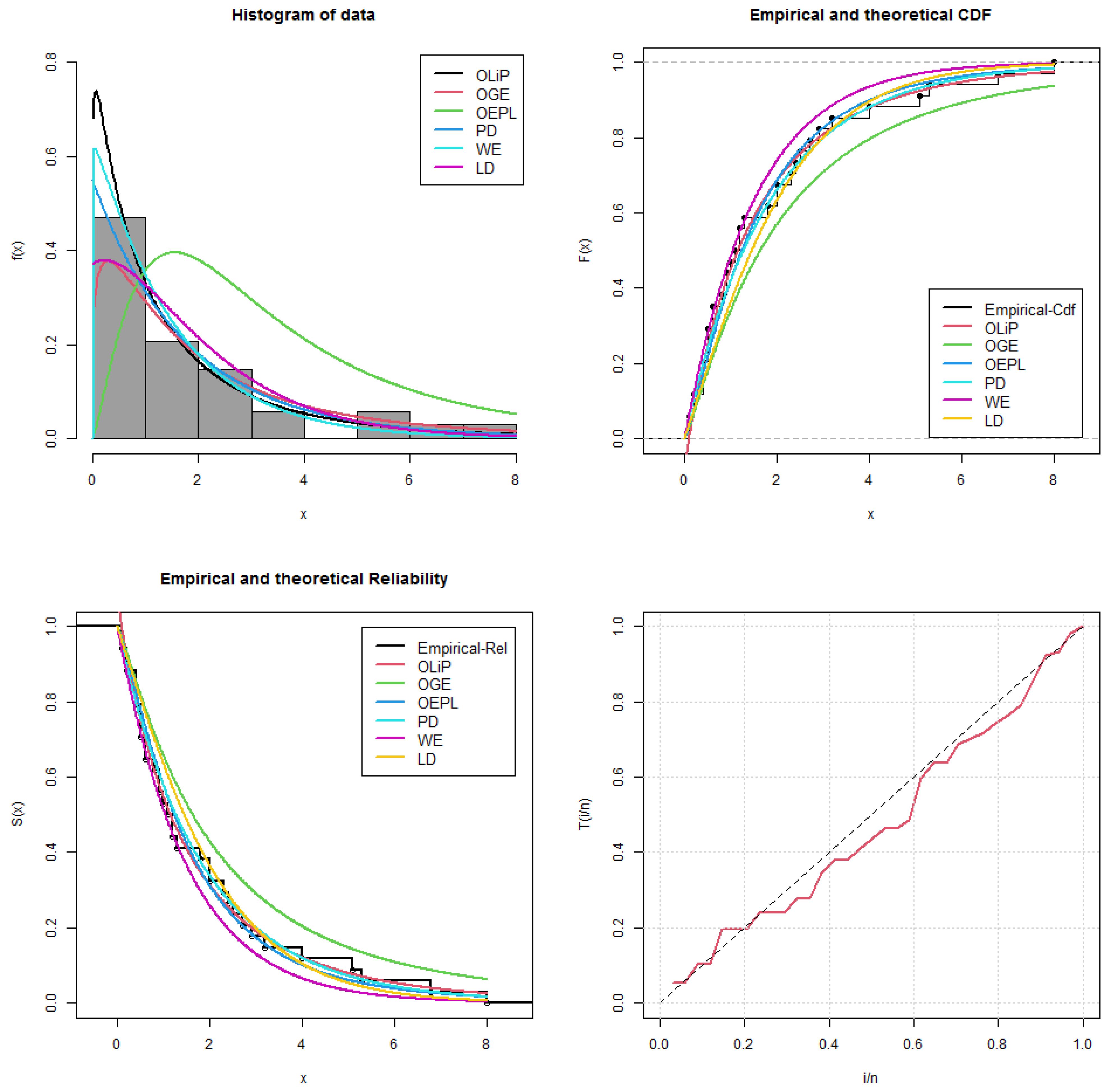
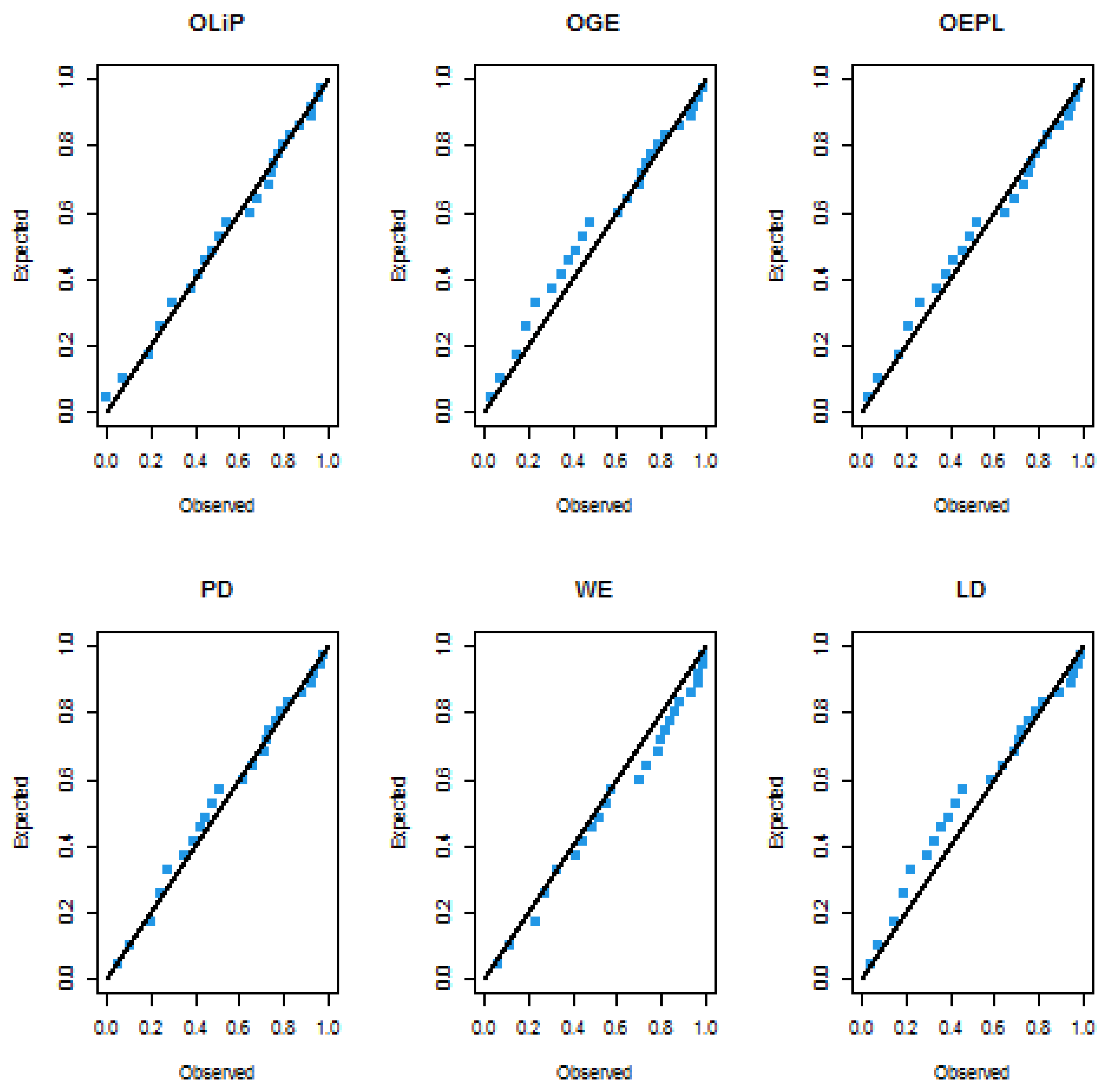
7.2.1. Vinyl Chloride Data Set
| 5.1 | 1.2 | 1.3 | 0.6 | 0.5 | 2.4 | 0.5 | 1.1 | 8.0 | 0.8 | 0.4 | 0.6 |
| 0.9 | 0.4 | 2.0 | 0.5 | 5.3 | 3.2 | 2.7 | 2.9 | 2.5 | 2.3 | 1.0 | 0.2 |
| 0.1 | 0.1 | 1.8 | 0.9 | 2.0 | 4.0 | 6.8 | 1.2 | 0.4 | 0.2 |
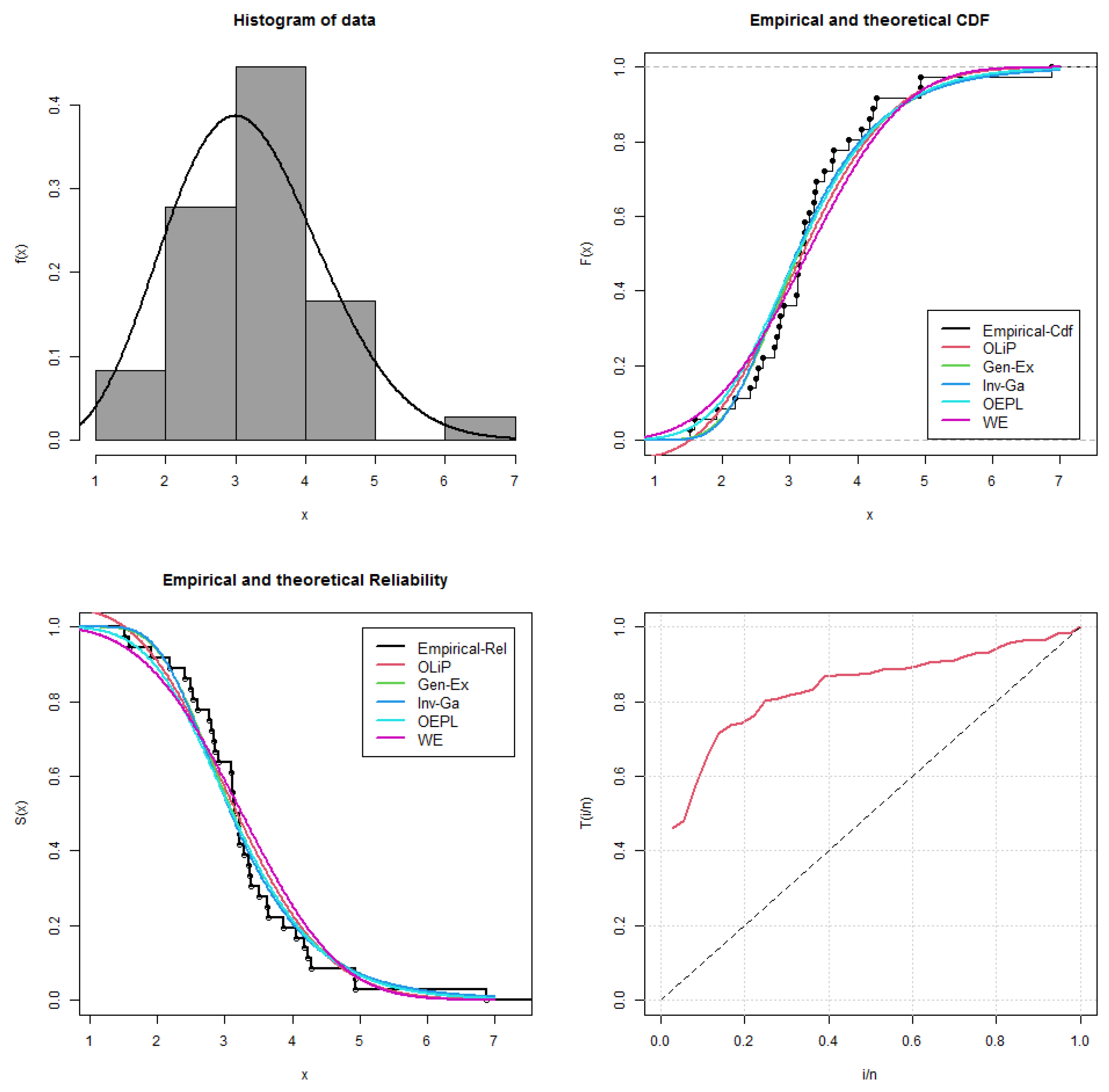
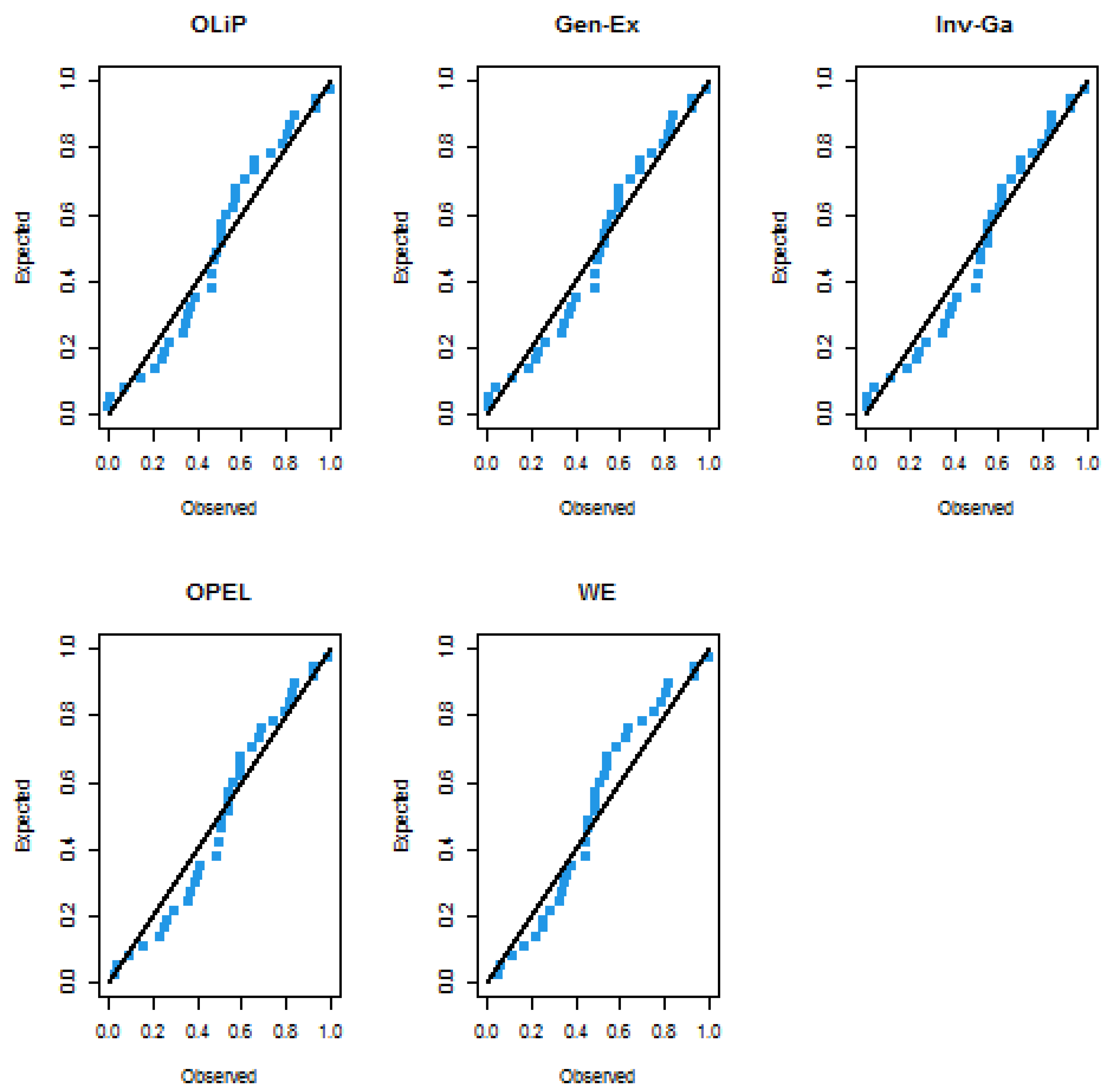
7.2.2. COVID-19 Data Set
| 3.1091 | 3.3825 | 3.1444 | 3.2135 | 2.4946 | 3.5146 | 4.9274 | 3.3769 | 6.8686 | 3.0914 | 4.9378 |
| 3.1091 | 3.2823 | 3.8594 | 4.0480 | 4.1685 | 3.6426, | 3.2110 | 2.8636 | 3.2218 | 2.907 | 3.6346 |
| 2.7957 | 4.2781 | 4.2202 | 1.5157 | 2.6029 | 3.3592 | 2.8349 | 3.1348 | 2.5261 | 1.5806 | |
| 2.7704 | 2.1901 | 2.4141 | 1.9048 |
8. Conclusions
Author Contributions
Funding
Data Availability Statement
Acknowledgments
Conflicts of Interest
References
- Johnson, N.L.; Kotz, S.; Balakrishnan, N. Beta distributions. In Continuous Univariate Distributions, 2nd ed.; John Wiley and Sons: New York, NY, USA, 1994; pp. 221–235. [Google Scholar]
- Johnson, N.L.; Kotz, S.; Balakrishnan, N. Continuous Univariate Distributions, Volume 2; John Wiley & Sons: New York, NY, USA, 1995; Volume 289. [Google Scholar]
- Gomes-Silva, F.S.; Percontini, A.; de Brito, E.; Ramos, M.W.; Venâncio, R.; Cordeiro, G.M. The odd Lindley-G family of distributions. Austrian J. Stat. 2017, 46, 65–87. [Google Scholar] [CrossRef]
- Taketomi, N.; Yamamoto, K.; Chesneau, C.; Emura, T. Parametric distributions for survival and reliability analyses, a review and historical sketch. Mathematics 2022, 10, 3907. [Google Scholar] [CrossRef]
- Shakil, M.; Kibria, B. On a family of life distributions based on generalized Pearson differential equation with applications in health statistics. J. Stat. Theory Appl. 2010, 9, 255–282. [Google Scholar]
- Shakil, M.; Kibria, B.G.; Singh, J.N. A new family of distributions based on the generalized Pearson differential equation with some applications. Austrian J. Stat. 2010, 39, 259–278. [Google Scholar] [CrossRef]
- Lindley, D.V. Fiducial distributions and Bayes’ theorem. J. R. Stat. Soc. Ser. (Methodol.) 1958, 20, 102–107. [Google Scholar] [CrossRef]
- Ghitany, M.E.; Atieh, B.; Nadarajah, S. Lindley distribution and its application. Math. Comput. Simul. 2008, 78, 493–506. [Google Scholar] [CrossRef]
- Zakerzadeh, H.; Dolati, A. Generalized lindley distribution. J. Math. Ext. 2009, 3, 13–25. [Google Scholar]
- Mazucheli, J.; Achcar, J.A. The Lindley distribution applied to competing risks lifetime data. Comput. Methods Programs Biomed. 2011, 104, 188–192. [Google Scholar] [CrossRef]
- Gupta, P.K.; Singh, B. Parameter estimation of Lindley distribution with hybrid censored data. Int. J. Syst. Assur. Eng. Manag. 2013, 4, 378–385. [Google Scholar] [CrossRef]
- Warahena-Liyanage, G.; Pararai, M. A generalized power Lindley distribution with applications. Asian J. Math. Appl. 2014, 2014, 23. [Google Scholar]
- Onyekwere, C.K.; Obulezi, O.J. Chris-Jerry Distribution and Its Applications. Asian J. Probab. Stat. 2022, 20, 16–30. [Google Scholar] [CrossRef]
- Anabike, I.C.; Igbokwe, C.P.; Onyekwere, C.K.; Obulezi, O.J. Inference on the Parameters of Zubair-Exponential Distribution with Application to Survival Times of Guinea Pigs. J. Adv. Math. Comput. Sci. 2023, 38, 12–35. [Google Scholar] [CrossRef]
- Shakil, M.; Khadim, A.; Saghir, A.; Ahsanullah, M.; Golam Kibria, B.; Ishaq Bhatti, M. Ratio of Two Independent Lindley Random Variables. J. Stat. Theory Appl. 2022, 21, 217–241. [Google Scholar] [CrossRef]
- Muse, A.H.; Tolba, A.H.; Fayad, E.; Abu Ali, O.A.; Nagy, M.; Yusuf, M. Modelling the COVID-19 mortality rate with a new versatile modification of the log-logistic distribution. Comput. Intell. Neurosci. 2021, 2021, 8640794. [Google Scholar] [CrossRef] [PubMed]
- Sankaran, M. 275. note: The discrete poisson-lindley distribution. Biometrics 1970, 26, 145–149. [Google Scholar] [CrossRef]
- Nadarajah, S.; Bakouch, H.S.; Tahmasbi, R. A generalized Lindley distribution. Sankhya B 2011, 73, 331–359. [Google Scholar] [CrossRef]
- Asgharzadeh, A.; Bakouch, H.S.; Esmaeili, L. Pareto Poisson–Lindley distribution with applications. J. Appl. Stat. 2013, 40, 1717–1734. [Google Scholar] [CrossRef]
- Ramadan, A.T.; Tolba, A.H.; El-Desouky, B.S. Generalized power Akshaya distribution and its applications. Open J. Model. Simul. 2021, 9, 323–338. [Google Scholar] [CrossRef]
- Lu, X.; Gui, W.; Yan, J. Acceptance sampling plans for half-normal distribution under truncated life tests. Am. J. Math. Manag. Sci. 2013, 32, 133–144. [Google Scholar] [CrossRef]
- Gui, W.; Zhang, S. Acceptance sampling plans based on truncated life tests for Gompertz distribution. J. Ind. Math. 2014, 2014, 7. [Google Scholar] [CrossRef]
- Al-Omari, A.I.F.; Koyuncu, N.; Alanzi, A.R.A. New acceptance sampling plans based on truncated life tests for Akash distribution with an application to electric carts data. IEEE Access 2020, 8, 201393–201403. [Google Scholar] [CrossRef]
- Yin, M.Z.; Zhu, Q.W.; Lü, X. Parameter estimation of the incubation period of COVID-19 based on the doubly interval-censored data model. Nonlinear Dyn. 2021, 106, 1347–1358. [Google Scholar] [CrossRef] [PubMed]
- Lü, X.; Hui, H.W.; Liu, F.F.; Bai, Y.L. Stability and optimal control strategies for a novel epidemic model of COVID-19. Nonlinear Dyn. 2021, 106, 1491–1507. [Google Scholar] [CrossRef] [PubMed]
- Pareto, V. Vilfredo Pareto; Sociologia: São Paulo, Brazil, 1848. [Google Scholar]
- Dagum distribution: Properties and different methods of estimation. Int. J. Stat. Probab. 2017, 6, 74–92. [CrossRef]
- Aldrich, J. RA Fisher and the making of maximum likelihood 1912–1922. Stat. Sci. 1997, 12, 162–176. [Google Scholar] [CrossRef]
- Albert, J. Bayesian Computation with R; Springer Science & Business Media: Berlin/Heidelberg, Germany, 2009. [Google Scholar]
- Gelman, A.; Carlin, J.B.; Stern, H.S.; Rubin, D.B. Bayesian Data Analysis; Chapman & Hall/CRC: Boca Raton, FL, USA, 2014; Volume 2. [Google Scholar]
- Swain, J.J.; Venkatraman, S.; Wilson, J.R. Least-squares estimation of distribution functions in Johnson’s translation system. J. Stat. Comput. Simul. 1988, 29, 271–297. [Google Scholar] [CrossRef]
- Mood, A.M. Introduction to the Theory of Statistics; McGraw Hill: New York, NY, USA, 1950. [Google Scholar]
- Varian, H.R. A Bayesian approach to real estate assessment. In Studies in Bayesian econometric and statistics in Honor of Leonard J. Savage; Wiley Online Library: Hoboken, NJ, USA, 1975; pp. 195–208. [Google Scholar]
- Doostparast, M.; Akbari, M.G.; Balakrishna, N. Bayesian analysis for the two-parameter Pareto distribution based on record values and times. J. Stat. Comput. Simul. 2011, 81, 1393–1403. [Google Scholar] [CrossRef]
- Calabria, R.; Pulcini, G. Point estimation under asymmetric loss functions for left-truncated exponential samples. Commun. Stat.-Theory Methods 1996, 25, 585–600. [Google Scholar] [CrossRef]
- Van Ravenzwaaij, D.; Cassey, P.; Brown, S.D. A simple introduction to Markov Chain Monte–Carlo sampling. Psychon. Bull. Rev. 2018, 25, 143–154. [Google Scholar] [CrossRef]
- Singh, S.; Tripathi, Y.M. Acceptance sampling plans for inverse Weibull distribution based on truncated life test. Life Cycle Reliab. Saf. Eng. 2017, 6, 169–178. [Google Scholar] [CrossRef]
- Bhaumik, D.K.; Kapur, K.; Gibbons, R.D. Testing parameters of a gamma distribution for small samples. Technometrics 2009, 51, 326–334. [Google Scholar] [CrossRef]
- Almetwally, E.M.; Alharbi, R.; Alnagar, D.; Hafez, E.H. A new inverted topp-leone distribution: Applications to the COVID-19 mortality rate in two different countries. Axioms 2021, 10, 25. [Google Scholar] [CrossRef]


| Model | MLEs | LL | AIC | CAIC | BIC | HQIC | KS | p-Value |
|---|---|---|---|---|---|---|---|---|
| OLiP | −53.35211 | 110.69382 | 111.08090 | 113.74651 | 111.73481 | 0.07506 | 0.99091 | |
| OGE | −55.14256 | 118.37101 | 119.75024 | 124.47631 | 120.45310 | 0.09767 | 0.90190 | |
| OEPL | −51.40121 | 112.83102 | 114.20711 | 118.93334 | 114.91315 | 0.10948 | 0.80981 | |
| PD | −55.44012 | 114.87893 | 115.26611 | 117.93162 | 115.92214 | 0.08138 | 0.97791 | |
| WE | −56.54913 | 117.0983 | 117.4854 | 120.1510 | 118.1393 | 0.12215 | 0.69071 | |
| LD | −56.32051 | 114.60647 | 114.73232 | 116.13360 | 115.12781 | 0.13262 | 0.58823 |
| Method | k | |||||
|---|---|---|---|---|---|---|
| Estimate | Std. Err | Estimate | Std. Err | Estimate | Std. Err | |
| MLE | 0.41717 | 0.08710 | 0.59434 | 0.09626 | 0.10000 | — |
| MPS | 0.30715 | 0.23391 | 0.57851 | 0.10591 | 0.05908 | 0.04616 |
| LSE | 0.30355 | 2.27254 | 0.57633 | 0.64212 | 0.05732 | 0.54144 |
| WLSE | 0.25304 | 0.10603 | 0.59156 | 0.03471 | 0.04691 | 0.02469 |
| CVME | 0.33629 | 2.31720 | 0.59318 | 0.68862 | 0.07319 | 0.58988 |
| ADE | 0.26275 | 0.56124 | 0.61308 | 0.21023 | 0.05551 | 0.13789 |
| RTADE | 0.29124 | 1.40565 | 0.60553 | 0.32673 | 0.06245 | 0.39334 |
| BE | 0.31990 | 0.03932 | 0.65006 | 0.04827 | 0.09620 | 0.00202 |
| Model | MLEs | LL | AIC | CAIC | BIC | HQIC | KS | p-Value |
|---|---|---|---|---|---|---|---|---|
| OLiP | −48.29042 | 100.58230 | 100.94591 | 103.74931 | 101.68772 | 0.12066 | 0.67101 | |
| Gen-Ex | −48.51342 | 101.02681 | 101.39050 | 104.19387 | 102.13220 | 0.12358 | 0.64156 | |
| Inv-Ga | −48.93963 | 101.87931 | 102.24286 | 105.04631 | 102.98461 | 0.13783 | 0.50092 | |
| OEPL | −57.38508 | 122.77016 | 124.06048 | 129.10424 | 124.98092 | 0.15500 | 0.35266 | |
| WE | −51.47427 | 106.94852 | 107.31224 | 110.115603 | 108.05385 | 0.14997 | 0.39296 | |
| Method | k | |||||
|---|---|---|---|---|---|---|
| Estimate | Std. Err | Estimate | Std. Err | Estimate | Std. Err | |
| MLE | 0.35251 | 0.11773 | 2.16421 | 0.32332 | 1.51570 | — |
| MPS | 0.25126 | 0.22176 | 2.06242 | 0.33171 | 1.26042 | 0.37469 |
| LSE | 0.05321 | 0.48064 | 3.11215 | 2.60681 | 1.05261 | 3.14173 |
| WLSE | 0.02459 | 0.00736 | 2.90658 | 0.14649 | 0.74861 | 0.09298 |
| CVME | 0.06561 | 0.74547 | 3.27890 | 2.76180 | 1.18667 | 4.10497 |
| ADE | 0.10695 | 0.58364 | 2.71285 | 0.75442 | 1.15982 | 2.14264 |
| RTADE | 0.61831 | 1.20303 | 2.22982 | 1.21607 | 1.91067 | 1.00573 |
| BE | 0.38171 | 0.05449 | 2.10173 | 0.22464 | 1.51337 | 0.06459 |
Disclaimer/Publisher’s Note: The statements, opinions and data contained in all publications are solely those of the individual author(s) and contributor(s) and not of MDPI and/or the editor(s). MDPI and/or the editor(s) disclaim responsibility for any injury to people or property resulting from any ideas, methods, instructions or products referred to in the content. |
© 2023 by the authors. Licensee MDPI, Basel, Switzerland. This article is an open access article distributed under the terms and conditions of the Creative Commons Attribution (CC BY) license (https://creativecommons.org/licenses/by/4.0/).
Share and Cite
Tolba, A.H.; Onyekwere, C.K.; El-Saeed, A.R.; Alsadat, N.; Alohali, H.; Obulezi, O.J. A New Distribution for Modeling Data with Increasing Hazard Rate: A Case of COVID-19 Pandemic and Vinyl Chloride Data. Sustainability 2023, 15, 12782. https://doi.org/10.3390/su151712782
Tolba AH, Onyekwere CK, El-Saeed AR, Alsadat N, Alohali H, Obulezi OJ. A New Distribution for Modeling Data with Increasing Hazard Rate: A Case of COVID-19 Pandemic and Vinyl Chloride Data. Sustainability. 2023; 15(17):12782. https://doi.org/10.3390/su151712782
Chicago/Turabian StyleTolba, Ahlam H., Chrisogonus K. Onyekwere, Ahmed R. El-Saeed, Najwan Alsadat, Hanan Alohali, and Okechukwu J. Obulezi. 2023. "A New Distribution for Modeling Data with Increasing Hazard Rate: A Case of COVID-19 Pandemic and Vinyl Chloride Data" Sustainability 15, no. 17: 12782. https://doi.org/10.3390/su151712782