GEV Analysis of Extreme Rainfall: Comparing Different Time Intervals to Analyse Model Response in Terms of Return Levels in the Study Area of Central Italy

Abstract

The extreme rainfall events of recent years in central Italy are producing an increase in hydrogeological risk, with disastrous flooding in terms of human lives and economic losses, as well as triggering landslide phenomena in correspondence with these events. A correct prediction of 100-year return levels could encourage better land planning, sizing works correctly according to the expected extreme events and managing emergencies more consciously through real-time alerts. In the recent period, it has been observed that the return levels predicted by the main forecasting methods for extreme rainfall events have turned out to be lower than observed within a few years. In this context, a model widely used in the literature, the generalised extreme value (GEV) with the “block maxima” approach, was used to assess the dependence of this model on the length of the collected precipitation time series and the possible addition of years with extreme events of great intensity. A total of 131 rainfall time series were collected from the Adriatic slope in central Italy comparing two periods: one characterised by 70 years of observations (1951–2020), the other by only 30 years (1991–2020). At the same time, a decision was made to analyse what the effect might be—in terms of the 100-year return level—of introducing an additional extreme event to the 1991–2020 historical series, in this case an event that actually occurred in the area on 15 September 2022. The results obtained were rather surprising, with a clear indication that the values of the 100-year return level calculated by GEV vary according to the length of the historical series examined. In particular, the shorter time series 1991–2020 provided higher return level values than those obtained from the 1951–2020 period; furthermore, the addition of the extreme event of 2022 generated even higher return level values. It follows that, as shown by the extreme precipitation events that have occurred in recent years, it is more appropriate to consider a rather short period because the ongoing climate change does not allow true estimates to be obtained using longer time series, which are preferred in the scientific literature, or possibly questioning the real reliability of the GEV model.

1. Introduction

Aim of the Study and State of the Art

Climate change is generating increasingly intense and frequent extreme rainfall events in much of the world. Central Italy is no exception either; in fact, a constancy in average precipitation amounts has been observed, but also a reduction in terms of rainy days [1]. Climate change is due to radiative forcings, which can be exogenous or endogenous, natural or man-made, such as changes in the solar radiation, Milankovic cycles, asteroid impacts, greenhouse gases, aerosols, land-use change and volcanic eruptions [2]. The abrupt climate change in recent years is almost exclusively due to anthropogenic causes and the emission of pollutants, which change the earth’s energy balance, producing a warming measurable in W/m² [3]. This increased energy in the atmosphere causes more intense and less predictable extreme events, which tend to put the hydrographic network in crisis, generating floods and generally increasing the hydrogeological risk [4,5]. In response to this type of problem, it is essential to be able to have reliable forecasts of the maximum precipitation values that we can expect in 100 years’ time, as this knowledge would allow us to take the correct countermeasures without underestimating them and without excessive economic expenditure [6]. The problem facing the institutions is knowing the maximum expected extreme precipitation event with a return time of 100 years (usually the most commonly used return time), since extreme events are occurring lately that have not been predicted at levels that would have return times of even more than 500 years [7]. The extreme value theory (EVT) deals with the study of extreme deviations from the central portion of a probability distribution, which makes it possible to predict return values [8]. The statistical models used to predict return levels can be univariate or bivariate, the univariate approach being represented by the peak-over-threshold fit to the generalised Pareto distribution (GPD), while the bivariate approach is represented by the block maxima fit to the generalised extreme value distribution (GEV). These two methods have different characteristics; although both are valid and reliable for the detection of return levels, GPD works better than GEV when the samples are small and therefore has greater independence from the sample size [9]. The main focus here was on the block maxima technique interpreted by means of the GEV distribution, which is widely used in the literature with excellent results [10]. In particular, the presence of non-stationarity in the time series leads to the use of numerical optimisation techniques, which allow the best estimation of the return level, such as maximum likelihood, which shows good results in non-stationary series in the literature [11]. The GEV method is used for the prediction of extreme events for each climatic factor, such as precipitation, temperature, wind and all those climatic factors, which could lead to hazards with their extreme manifestation [12,13]; however, the GEV is also widely used in economics, especially aimed at predicting rather negative economic scenarios or risks and in engineering [14,15]. In any case, the most widespread application of the GEV method is the definition of maximum rainfall return values due to the reliability of the forecast, although it sometimes seems to be penalised, as some research has shown, by estimates based on short time series because they make it difficult to estimate the shape parameter and also due to possible errors in the measurements [16]. It is well known that measurement errors are possible both when analysing weather stations, due to a lack of quality control, and also when using satellite data, which are not always reliable or calibrated in the study area [17]. In this context, it has been shown that shorter data sets using the GEV methodology compared to longer data sets show higher return values, which sometimes seem to be more in line with the actual values that can then be seen in the long run [18]. In the literature, we find examples of distributions such as Gumbel’s, which underestimate extreme events, something that should not be the case with GEV, which, on the other hand, based on three different distributions (Gumbel, Frechet, Weibull), usually succeeds in obtaining values that are more in line with reality, using the distribution that best fits the data set [19]. In essence, this study starts from the observation that the dependence of the return value calculated with the GEV method from a longer or shorter data record is not yet sufficiently researched in the scientific literature on the subject, although it could be decisive in the choice of the length of the time series. This is the motivation for evaluating, with the same GEV methodology, time series with different reference periods in the same area (1991–2020 and 1951–2020), as well as for evaluating the influence that the addition of an extreme event, which actually occurred (15 September 2022), can have on the variation of the return value estimate within a 100-year period. In addition, it is important to assess the reliability of the estimate of the extreme precipitation event in relation to what actually happens in order to understand whether the correctness of the method in forecasting may be affected by the climate changes, which are leading to increasingly frequent and more intense extreme events [20]. These are highly topical issues and important due to the impact they have on the populations that reside in certain territories, as they contribute to a more accurate assessment of extreme precipitation events, which can lead to critical issues, such as those of slope instability or flooding [21,22]. Therefore, in order to mitigate the effects of climate change on the territory, it is advisable to know the exact intensity of the extreme precipitation event that may occur with a given return time, with the aim of correctly sizing the mitigation structures or those present in areas at risk in order to ensure decisive adaptation strategies without unnecessary expenditure of resources [23]. Furthermore, predicting the correct 100-year return levels of rainfall would allow for a correct assessment of sustainability, both in environmental and economic terms.

2. Study Area and Method

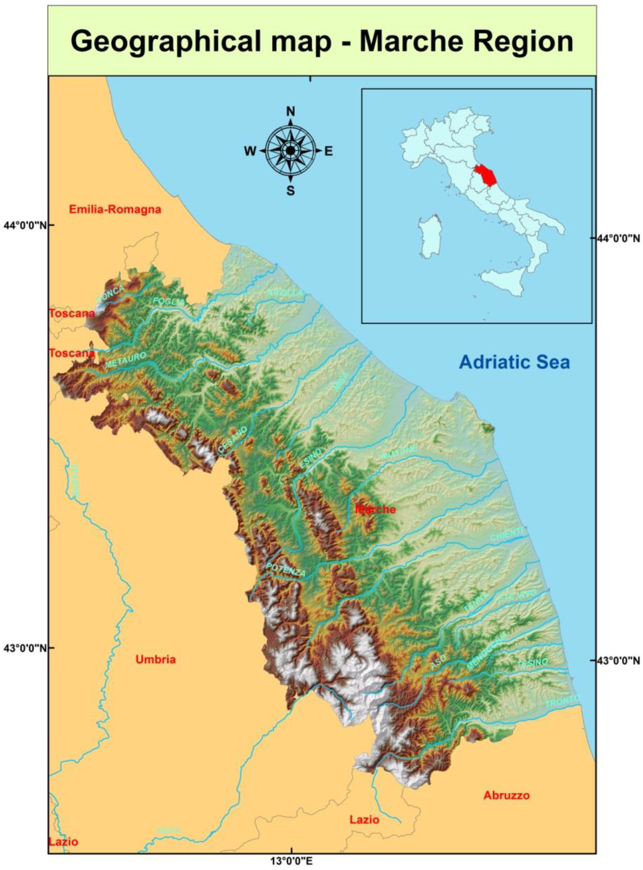
2.1. Study Area

The Italian peninsula is undergoing a general increase in the frequency of extreme events; in this case, the middle Adriatic side of central Italy was considered [24]. The study area was chosen because of an extreme event that occurred on 15 and 16 September 2022, which disproved the return value estimates present in the area up to that time; thus, the real reliability of the GEV method for forecasting extreme precipitation events in the area was assessed. The chosen area, corresponding to the Marche region, has an areal extension of 9694 km²; its territory is one-third mountainous, while the remaining two-thirds consists of a very wide pre-Apennine hilly belt sloping down to the sea, with the few plains located near the coast and along the low alluvial valleys of the main rivers (Figure 1). The morphology of the region presents a sharp contrast between the predominantly mountainous western part and the essentially hilly eastern part down to the Adriatic coast. From an orographic point of view, the region is characterised by the Umbro-Marchigiano Apennines in the western part with a NNE/SSW development direction, such that it assumes an arcuate trend with convexity towards the east, whose highest peak is Monte Vettore (2476 m a.s.l.).

Climatically, this complex morphology of the territory favours the presence of a wide range of climates, which, following the Koppen–Geiger classification, range between Csa, Cfa, Cfb, Cfc and Dsc on the major peaks [25]. There are four air masses, which characterise this area, also due to its morphology:

• Continental arctic cold: It develops in northern Russia in the area of Siberia; this air mass can affect Italy from late October to April, and it represents the coldest air mass, which can affect the Italian territory.
• Continental polar cold: Cold, dry air mass from southern Russia originating in the Balkan area.
• Continental tropical warm: Hot, dry mass of air originating from arid and desert areas from the southern belt; it represents the warmest air mass affecting Italy.
• Maritime tropical warm: Air mass from the southwest in the Atlantic Ocean; in winter, it is mild and humid, while in summer, it becomes hot and muggy.

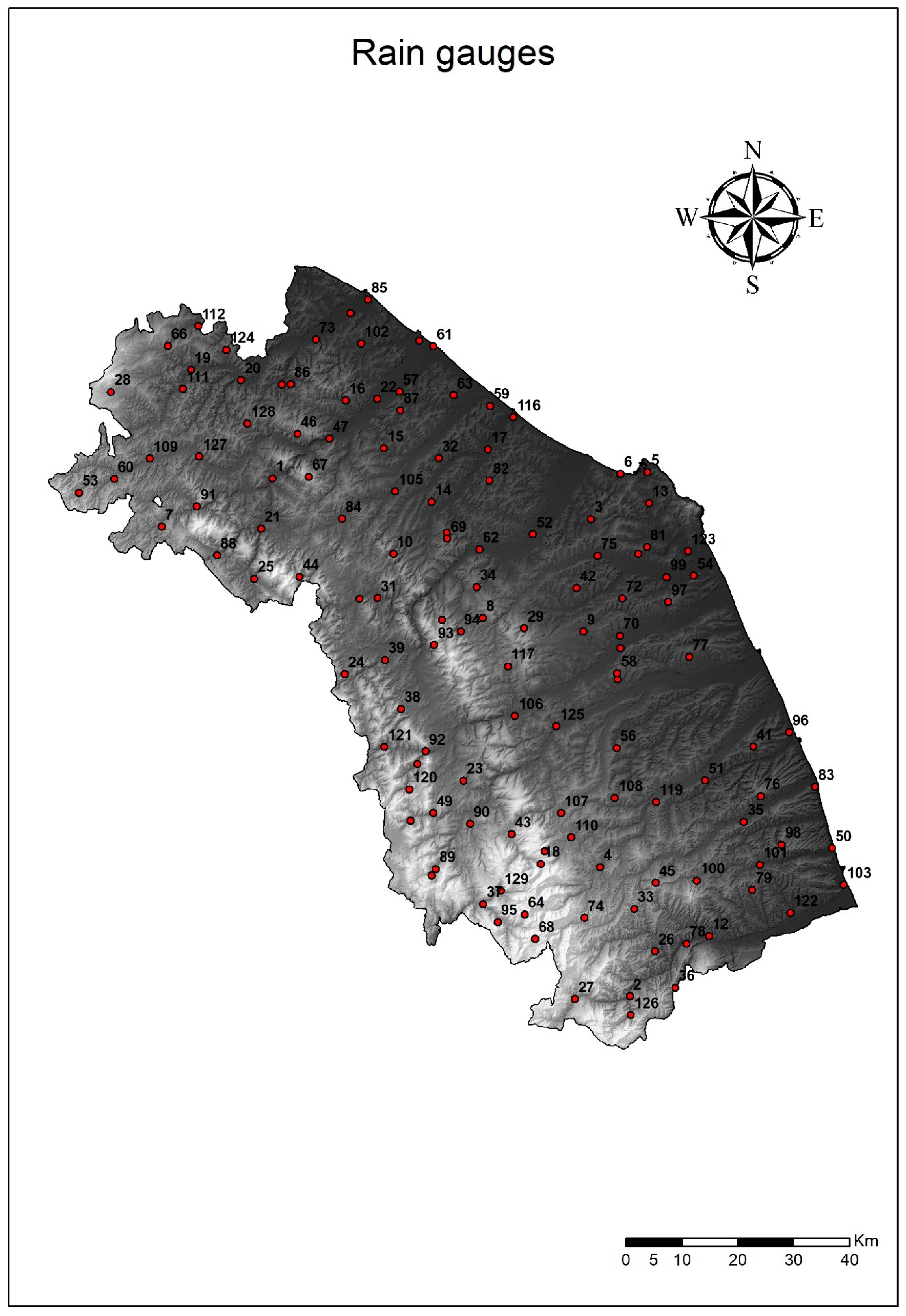
2.2. Weather Stations

The rain gauge data were collected by Sistema Informativo Regionale Meteo-Idro-Pluviometrico (SIRMIP), an online climate data storage system operated by the Civil Protection’s Multi-Hazard Functional Centre. There were 131 rain gauges used for the analysis (Figure 2), active for all or part of the period from 1951 to 2022, with 1, 3, 6, 12 and 24 h heavy rainfall data.

The knowledge of the amount of data available for each weather station collected is essential information for the evaluation of the research and its reproducibility, especially when, as in this case, there are many different existence intervals (

Table 1. Weather stations and collected data: Code = unique code of each weather station, which can be found in the map in Figure 2; W.S. = name of the weather station; Lifetime = period of existence of the weather station.

Code	W.S.	Lifetime
1	Acqualagna	1991–2005/2007–2020
2	Acquasanta	1991–2007/2012–2020
3	Agugliano	2008–2020
4	Amandola	1991–2014/2016–2020
5	Ancona Regione	2008–2020
6	Ancona Torrette	1991–2020
7	Apecchio	2008–2020
8	Apiro	1991–2008
9	Appignano	2008–2020
10	Arcevia	1951–2020/2022
11	Arquata del Tronto	1991–2014/2016–2020
12	Ascoli Piceno	1951–2003/2006–2014
13	Baraccola	1991–2007/2010–2020
14	Barbara	1991–2020/2022
15	Barchi	1991–2007
16	Bargni	1951–1959/1961/1964–1971/1973–2007
17	Bettolelle	2008–2020
18	Bolognola	1991–2020
19	Bronzo	2008–2020
20	Ca’ Mazzasette	2008–2018
21	Cagli	1991–2014/2019–2020
22	Calcinelli	1991–2014
23	Camerino	1991–1996/2008–2020
24	Campodiegoli	1991–2020
25	Cantiano	1951–2020/2022
26	Capo di Colle	1991–2007
27	Capodacqua	1991–2005/2007/2009–2020
28	Carpegna	1991–2020
29	Cingoli	1991–2008/2010–2020
30	Colle	2008/2010–2020/2022
31	Colleponi	2008–2020
32	Corinaldo	1991–2020
33	Croce di Casale	1991–2014
34	Cupramontana	1991–2020
35	Diga di Carassai	1951–1965/1968/1984–2007
36	Diga di Talvacchia	1991–2007
37	Endesa	2008–2020
38	Esanatoglia convento	2008/2010–2020
39	Fabriano	1952–2009/2011/2014–2020
40	Fano	1991–2014
41	Fermo	1991–1999/2001–2020
42	Filottrano	1991–2008/2010–2012/2016–2020
43	Fiume di Fiastra	1991–2020
44	Fonte Avellana	1991–2004/2008–2020/2022
45	Force	2008–2020
46	Foresta della Cesana	1991–2006/2010–2020
47	Fossombrone	1991–2017/2019–2020
48	Gallo	2008–2020
49	Gelagna Alta	1993/1996–2015/2018–2020
50	Grottammare	2008–2020
51	Grottazzolina	2008–2020
52	Jesi	1953–1961/1963–2020
53	Lamoli	1991/1993–2007
54	Loreto	1991–2020
55	Lornano	1991–2016
56	Loro Piceno	1951–1962/1964/1966–1967/1969–1972/1991–2020
57	Lucrezia	2008–2020
58	Macerata Montalbano	2009–2020
59	Marotta Cesano	2008–2020
60	Mercatello	1991–2010
61	Metaurilia	2008–2014/2017–2020
62	Moie	1951–2020
63	Mondolfo	1991–2007
64	Monte Bove Sud	2008–2020
65	Monte Cavallo	2008–2020
66	Monte Grimano Terme	2008–2020
67	Monte Paganuccio	2009–2020
68	Monte Prata	2008–2020
69	Montecarotto	1991–2007
70	Montecassiano	1991–2007
71	Montecchio	2011–2020
72	Montefano	2008–2020
73	Montelabbate	2008–2020
74	Montemonaco	1991–2020
75	Montepolesco	2009–2020
76	Monterubbiano	1992–2007
77	Morrovalle	1998–2014
78	Mozzano	2008–2020
79	Offida	1991–2002
80	Osimo	1991–2013
81	Osimo Monteragolo	2008–2020
82	Ostra	1991/1993–2007
83	Pedaso	1951–1969/1971–2007
84	Pergola	1991–2020
85	Pesaro	1991–2001/2008–2020
86	Petriano	1991–2007
87	Piagge	1991–1994/1996–2020
88	Pianello di Cagli	1991–2020
89	Pie’ del Sasso	1991–2007
90	Pieve Bovigliana	1991–1994/1996–2020
91	Piobbico	1952–1961/1963–1973/1991–2014/2016–2020
92	Pioraco	1991–2020
93	Poggio S. Romualdo	1991–2007
94	Poggio San Vicino	2010–2020
95	Ponte Tavola	2008–2020
96	Porto S. Elpidio	1951–1964/1967–1978/1980/2020
97	Recanati	1991–2020
98	Ripatransone	1991–2020
99	Rostighello	2010–2020
100	Rotella	2008–2020
101	S. Maria Goretti	2010–2020
102	S. Maria in Arzilla	2008–2020
103	San Benedetto	2008–2020
104	San Giovanni	2008–2020
105	San Lorenzo in Campo	1991–2008/2010–2020
106	San Severino Marche	2008–2020
107	Santa Maria di Pieca	1999–2020
108	Sant’Angelo in Pontano	1999–2020
109	Sant’Angelo in Vado	1991–2020
110	Sarnano	1954–1973/1991–2007
111	Sassocorvaro	1951–1963/1965–1966/1968–1972/1991–2007
112	Sassofeltrio	2008–2016/2018–2020
113	Sassoferrato	1991–2020
114	Sassotetto	2008–2020
115	Sefro	2010–2020
116	Senigallia	1991–2020
117	Serralta	1991–2001/2008–2020
118	Serravalle di Chienti	1991–2013/2015–2020
119	Servigliano	1991–2014/2016–2020
120	Sorti	1992–2020
121	Spindoli	2010–2020
122	Spinetoli	1991–2020
123	Svarchi	2010–2020
124	Tavoleto	1991–2008/2010–2020
125	Tolentino	1991–1996/1998–2008/2010–2020
126	Umito	2008–2020
127	Urbania	1991–2016/2018–2020
128	Urbino	1991–2020
129	Ussita	2008–2020
130	Villa Fastiggi	2008–2020
131	Villa Potenza	2008–2020

).

In particular, three different periods were selected: the first from 1951 to 2020, the second from 1991 to 2020, the third from 1991 to 2022. These three different periods were chosen in order to be able to make appropriate comparisons between 100-year return levels, between longer (1951–2020) and shorter (1991–2020) periods, as well as to assess the effect of introducing into the data set the extreme events of September 2022, only in part of the regional area, i.e., the area affected by the extreme event in question.

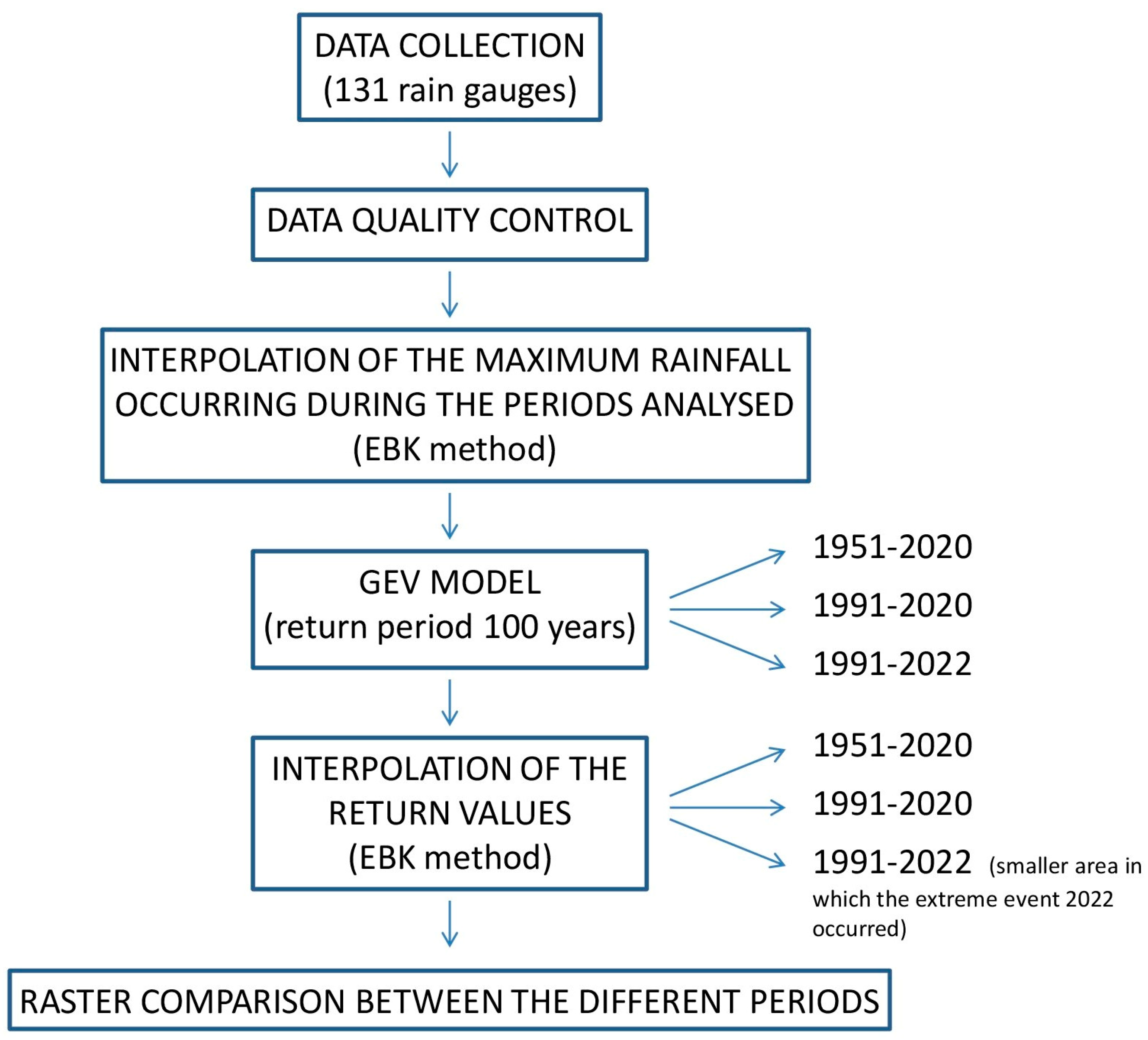
2.3. Flow Chart of the Analysis

For a better understanding of the analysis, a flow chart was created summarising the steps needed to achieve the results obtained (Figure 3).

After collecting rainfall data at hourly time steps, analyses were performed to check the quality of the data through validation and homogenisation processes. The data were then merged, and a maximum value for each year of analysis was obtained for the 1, 3, 6, 12, 24 h intervals. Then, the maximum values obtained were spatialised over the study surface for both periods 1951–2020 and 1991–2020, so that we could actually understand what maximum values occurred in the study area over the past several years. Subsequently, an analysis of extreme precipitation events was carried out to obtain 100-year return levels through the GEV model for each individual rainfall station. The GEV analysis was followed by geostatistical interpolation of the study area for all periods analysed, while in the case of the 1991–2022 period, it was spatialised only in the areas that were subjected to this event. Finally, the difference between the interpolation of return values over the periods 1951–2020 and 1991–2020 was evaluated in order to understand the effects that period length may have on return levels and what might be the most reliable interval to consider.

2.4. Software

The software used for the analysis of extreme events in this research consisted of R, which made it possible to apply the GEV method through the use of the specific package “in2extRemes”, and ArcGis 10.8, which was indispensable for the cartographic representation and interpolation of the data. The “in2extRemes” package provides general functions for analysing extreme events; in particular, it uses extreme value analysis (EVA), which refers to the use of the extreme value theory (EVT) for the analysis of data involving rare or low-probability events, such as maximum annual precipitation [26]. ArcGis 10.8 is a software, which creates, manages, analyses and maps georeferenced data and is thus necessary in this case to enable faster understanding, and with its Geostatistical Analyst package, it allows the interpolation of point data with deterministic or geostatistical techniques [27,28].

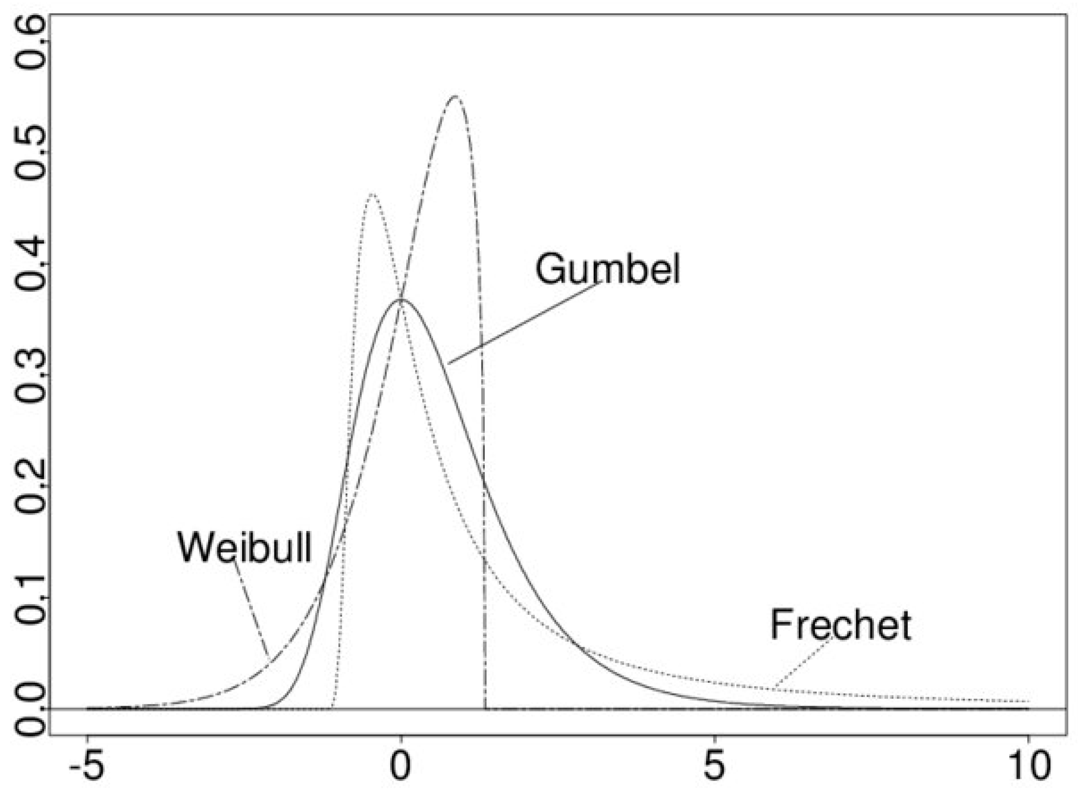
2.5. GEV Model and Statistical Interpolation Techniques

The extreme value theory deals with the stochasticity of natural variability by describing extreme events with respect to a probability of occurrence. GEV examines the distribution of block maxima (a block is defined as a fixed period of time, e.g., one year); depending on the shape parameter, a Gumbel, Frechet or Weibull distribution will be produced (Figure 4).

These distributions were reformulated with the shape distribution function:

$$f\left(x\right)=\left\{\begin{array}{c}\frac{1}{\sigma }\exp {(-(1+kz)}^{-1/k}{(1+kz)}^{-1-1/k}, k\ne 0\\ \frac{1}{\sigma }\exp \left(-z-\mathit{exp}\left(-z\right)\right), k=0\end{array}\right.$$

(1)

where $z=\frac{(x-\mu )}{\sigma }$.

The GEV model has three parameters: a location parameter μ, a scale parameter σ and a shape parameter k. The range of definition of GEV depends on k:

$$\genfrac{}{}{0pt}{}{1+k\frac{(x-\mu )}{\sigma }>0 k\ne 0}{-\infty <x<+\infty k=0}$$

(2)

The shape parameter k sets three types of distribution:

k = 0: Gumbel distribution;

k > 0: Frechet distribution;

k < 0: Weibull distribution.

Grouping the three extreme value distributions into a single model greatly simplifies statistical implementations. Through inference of the shape parameter, it is the data themselves that determine the most appropriate tail type, and consequently, there is no need to make subjective judgments about which family of extreme values to adopt. The values of the parameters were obtained with the “maximum likelihood estimation” method (MLE), which allows us to calculate the probability of observing the sample as the parameter θ changes. It follows that the likelihood function L(θ) should be seen as a function of parameter θ only and that it allows the parameter to be estimated only after observing the sample. Operationally, through the GEV model, the return period $1/p$ was obtained by the maximum likelihood estimation of $z_p$ for a probability between 0 and 1 in the following way:

$$z_p=\mu +\frac{\sigma }{k}\left({\left[-\log (1-p)\right]}^{-k}-1\right)$$

(3)

In addition, the confidence interval for each specific return time was also calculated, again parameterising the GEV model, such that z_p was one of the model parameters as follows:

$$\mu =z_p+\frac{\sigma }{k}\left\{1-{\left[-\log (1-p)\right]}^{-k}\right\}$$

(4)

The in2extRemes package generates four resulting graphs, which allow one to understand how well the model fits the data distribution but also the level of return at different time intervals (Figure 5). The quantile plot compares quantiles derived from the empirical distribution of the observed data (empirical quantiles) against the theoretical quantiles calculated from the estimated model (model quantiles). The arrangement of the points along the diagonal line is indicative of a good fit of the model to the data. The empirical quantile differs from the model quantile, in that in it, the empirical quantiles present on the x-axis are compared with the quantiles calculated on a synthetic data set simulated by the estimated model. The empirical quantile is generally less informative than the model quantile and is characterised by a lower proximity of the data to the diagonal line. The frequency histogram shows the empirical frequency distribution of the data (approximated using a non-parametric kernel-type interpolator) against the theoretical density curve of the model (blue line); the overlap of the two curves confirms the good fit of the model to the data. The return period plot depicts the return levels; the solid black line represents the return levels estimated by the model, while the dots represent the data observed arranged according to the corresponding return time (x-axis). The bands of confidence (dashed lines in grey) are calculated with the delta method: as the times increase the return times, the confidence intervals become wider and wider, reflecting the greater uncertainty, which accompanies the estimation process as the available information decreases. In the graph, the values on the x-axis are represented on a logarithmic scale in order to show the trend of the estimated curve.

At the end of the GEV procedure, the return levels at 100 years were identified for each rain gauge analysed; then, these values were used to perform an interpolation analysis all over the study area for all the periods investigated: 1951–2020, 1991–2020 and 1991–2022 (only for a small area). Interpolation is the process of obtaining a value for a variable of interest at a point where there is no sampling using data from locations close to it. In this case, a geostatistical method was chosen for the spatialisation of the data; geostatistical methods have the merit of quantifying the uncertainty associated with the interpolated values by making estimates of the error and providing insight into the predictive ability of the model. Geostatistical methods involve kriging, which is based on Tobler’s first law—“everything is related to everything else, but the nearest are more related than the distant”—and they are based on measuring the spatial autocorrelation of the values. Kriging uses the semivariogram, which is a function of the distance and direction separating two locations, to quantify the spatial dependence of the data with the aim of minimising the mean square error. The semivariogram makes it possible to examine the spatial correlation between pairs of values; the x-axis shows the planimetric distance between pairs of stations, while the y-axis shows the difference between values. The mathematical formula to determine the values of the y-axis is as follows:

$$\gamma \left(s_i,s_j\right)=\frac{1}{2}var\left(Z\left(s_i\right)-Z\left(s_j\right)\right)$$

(5)

$Z\left(s_i\right)-Z\left(s_j\right)$ = subtraction between a pair of neighbouring values.

The semivariogram is described by certain features (Figure 6):

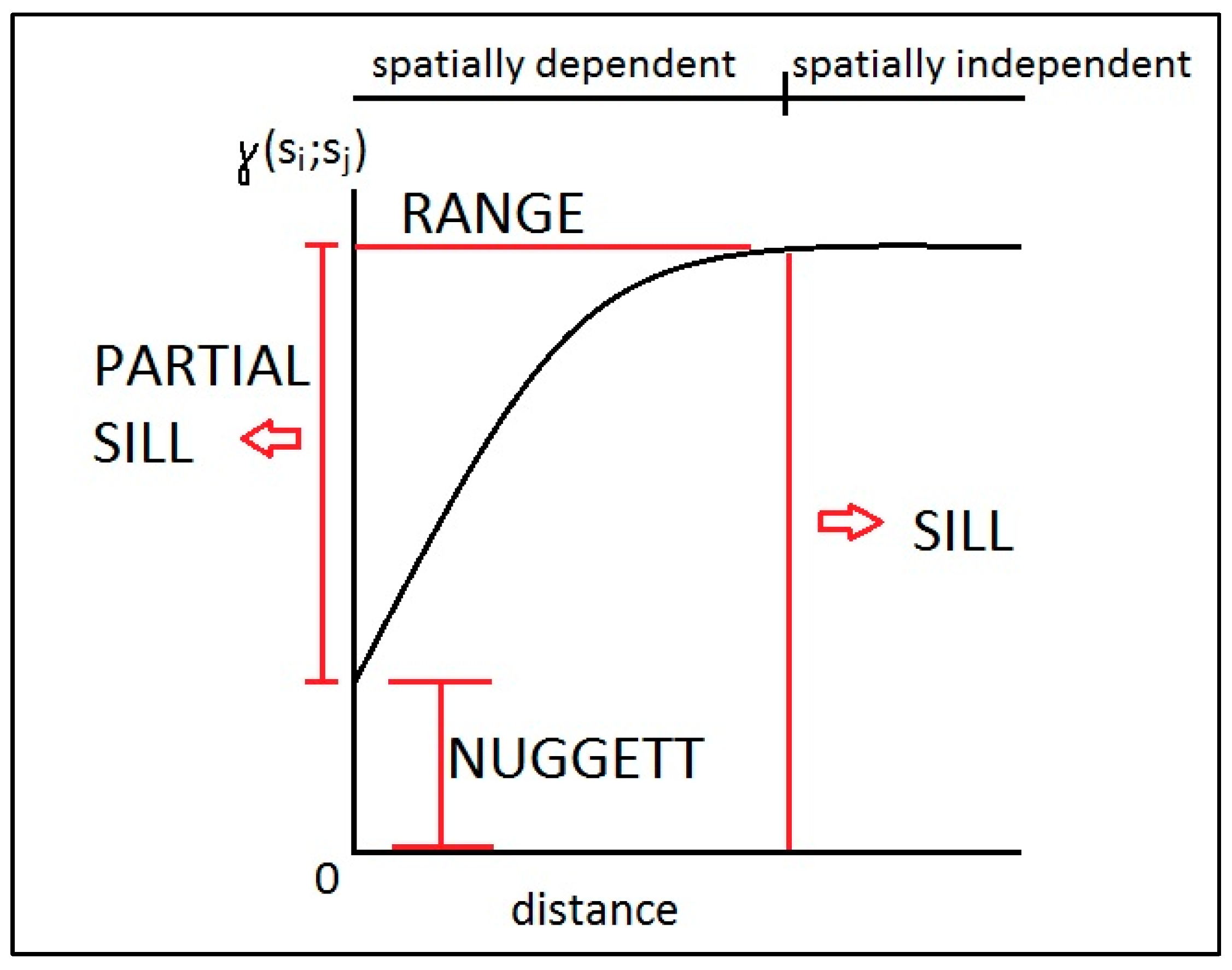
• Range: This is the point at which the semivariogram flattens out and consequently signals the end of autocorrelation between pairs of values.
• Nugget: This is the value of y (other than zero) when x is zero. It often indicates measurement error or variations at distances smaller than the sampling distances.
• Sill: This is the value of the y-axis when the range flattens out.

In addition to different types of kriging, there are also various models (circular, spherical, pentaspherical, Gaussian, etc.), which interpret the course of the semivariogram more or less well depending on the case. In a semivariogram, the goodness of the interpolation is assessed by means of certain statistical indices, which show the magnitude of the errors and the accuracy of the prediction. These indices include the following:

Mean error = the difference between the average of observed and predicted values; it follows that a value close to zero assumes a good prediction.

$$\frac{\sum _{i=1}^{n }[\widehat{\widehat{Z}}\left(s_i\right)-z(s_i)]}{n}$$

(6)

$\widehat{Z}\left(s_i\right)$ = measured value at location $s_i$;

$z\left(s_i\right)$ = predicted value at $s_i$;

$n$ = number of weather stations.

Root of mean square error = the square root of the ratio of the sum of the squares of the deviations (difference between the measured value and the predicted value) to the number of deviations. This parameter is not absolute but scale-dependent, so any comparison is difficult.

$$\sqrt{\frac{{\sum _{i=1}^n[\widehat{Z}\left(s_i\right)-z(s_i)]}^2}{n}}$$

(7)

Standard error = this represents the standard deviation from the mean; a value close to zero indicates a low error in estimating the variability of the distribution.

$$\sqrt{\frac{\sum _{i=1}^n{\widehat{\sigma }}^2(s_i)}{n}}$$

(8)

Standardised mean error = similar to the mean error; however, it differs from it, in that it standardises one random variable with mean x and variance σ² to another with 0 mean and variance equal to 1 in order to allow a comparison of variables with different orders of magnitude.

$$\frac{\sum _{i=1}^{n }[\widehat{\widehat{Z}}\left(s_i\right)-z(s_i)]/\widehat{\sigma }(s_i)}{n}$$

(9)

Root of standardised mean square error = the root of the mean square error, which was standardised with the method described in the case of the standardised mean error. A value close to 1 is desirable, keeping in mind that a higher value indicates an underestimation of model variability, and a lower value corresponds to an overestimation of it.

$$\frac{\sum _{i=1}^{n }[\widehat{\widehat{Z}}\left(s_i\right)-z(s_i)]/\widehat{\sigma }(s_i)}{n}$$

(10)

In the present study, various types of interpolation were tested: ordinary kriging (OK), simple kriging (SK), co-kriging (CK) and empirical Bayesian kriging (EBK). In particular, the best results were obtained with the EBK, as the CK did not show a sufficiently strong relationship between the dependent variable (extreme precipitation event) and the independent variable; in particular, altitude, distance from the sea and also latitude were used as independent variables. EBK is an iterative method and differs from classical kriging methods, in that it takes into account the error introduced by estimating the semivariogram model, which is achieved by estimating and using many semivariogram models rather than a single semivariogram. EBK consists of repeated simulations to identify the model, which best approximates the semivariogram obtained from the data; this process creates a spectrum of semivariograms, where each semivariogram is an estimate of the true semivariogram. EBK also differs from other kriging methods by accounting for the error introduced by estimating the underlying semivariogram; other kriging methods underestimate the standard errors of prediction [29].

3. Results

The two periods 1991–2020 and 1951–2020 were studied in order to understand the differences in return value between the study with only 30 years of data and the study with 70 years of data during the most studied time intervals, i.e., at 1, 3, 6, 12, 24 h. In order to make this comparison, the maximum annual precipitation was analysed and spatialised to assess the correspondence between the actual value measured in the last period (1991–2020)—because this is the period where an increasing trend of extreme events is being observed—and the 100-year return value.

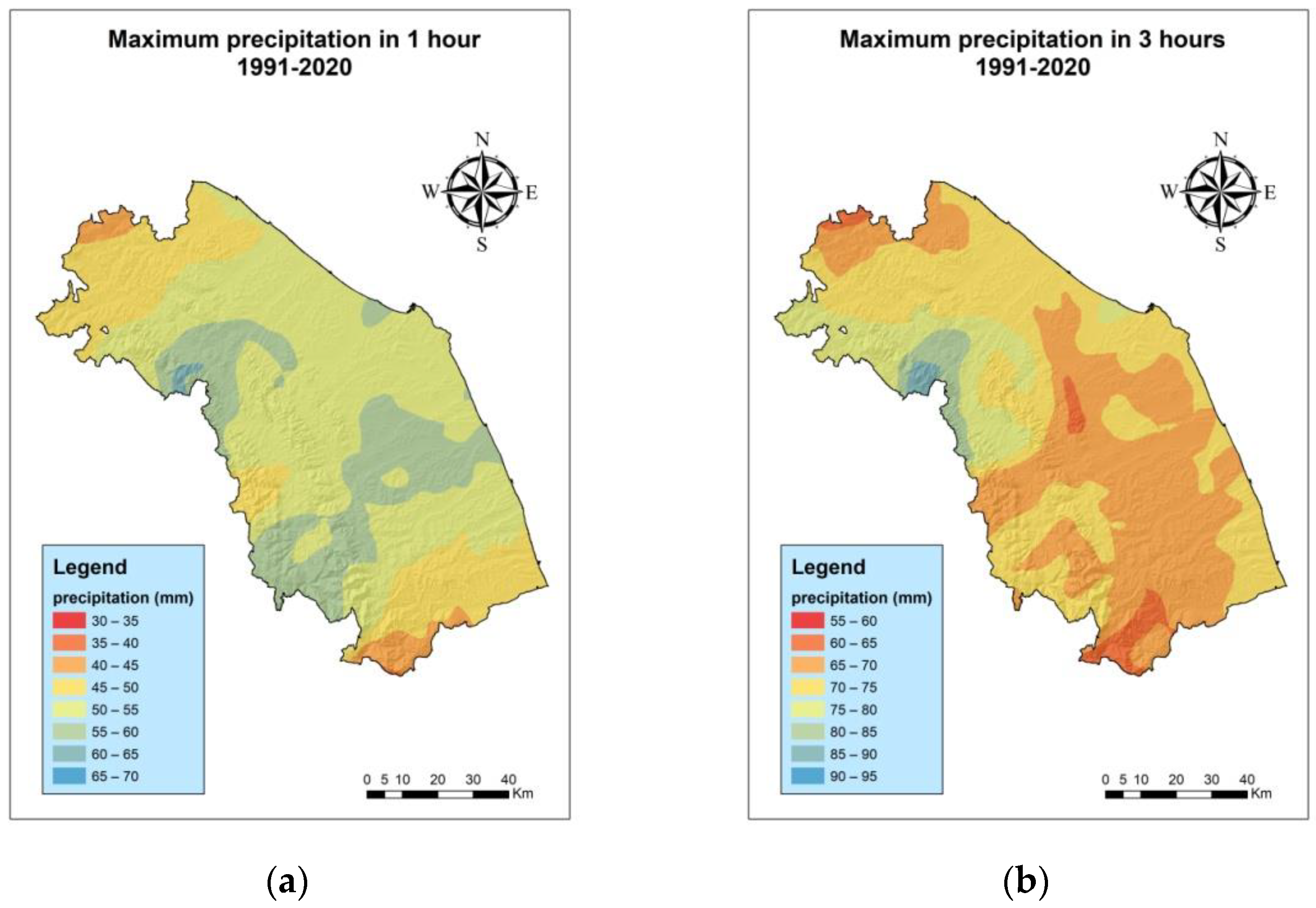
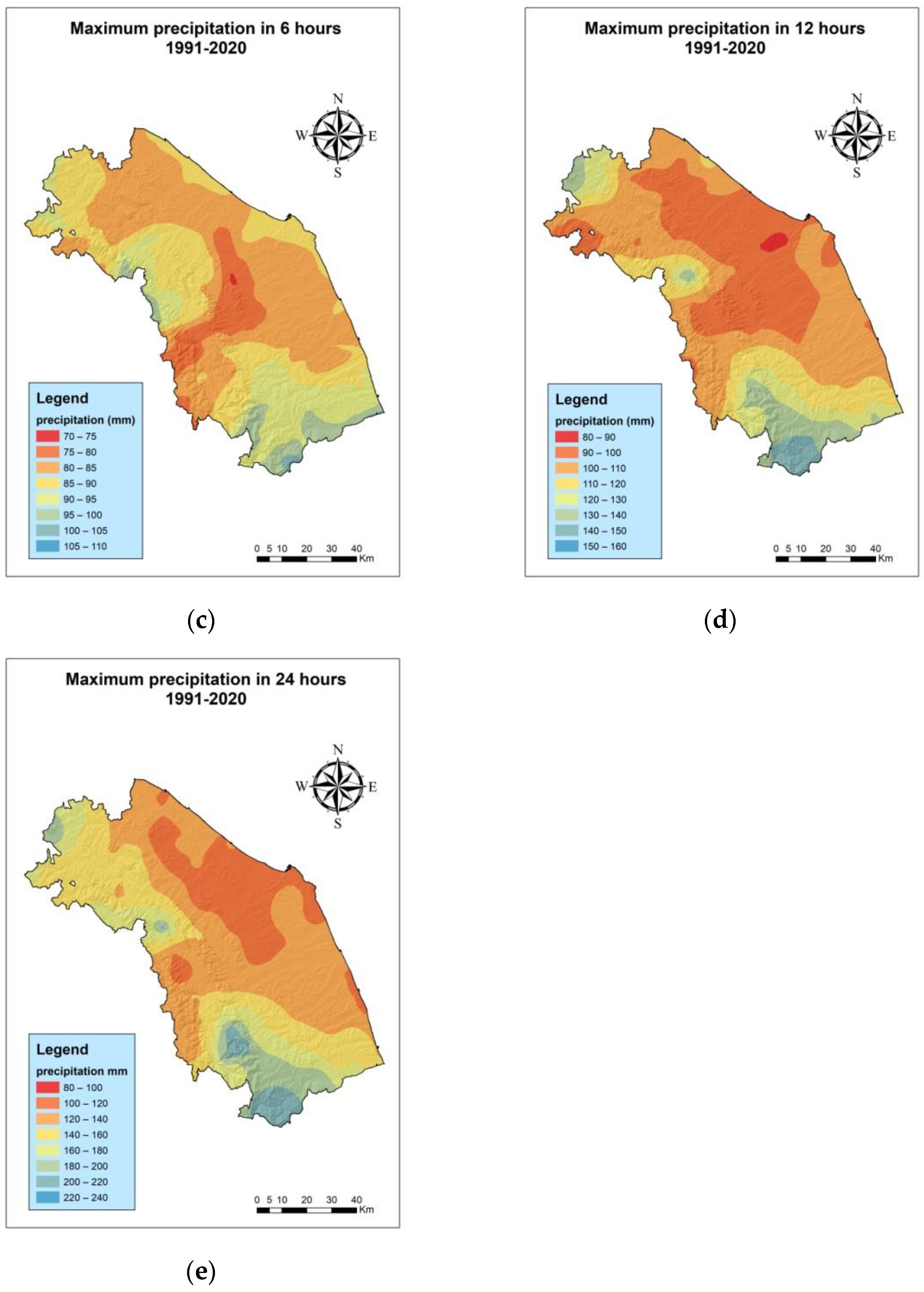
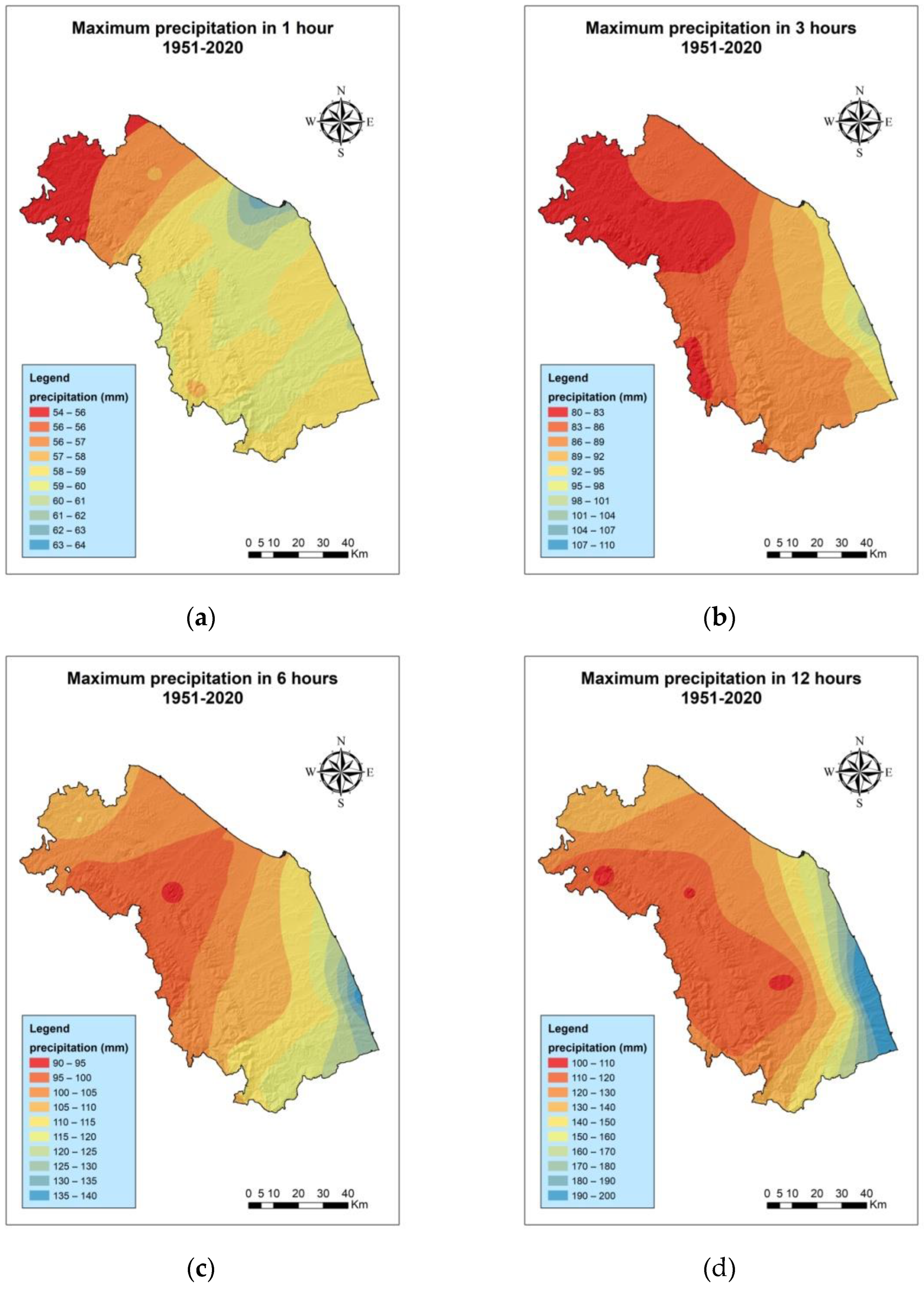
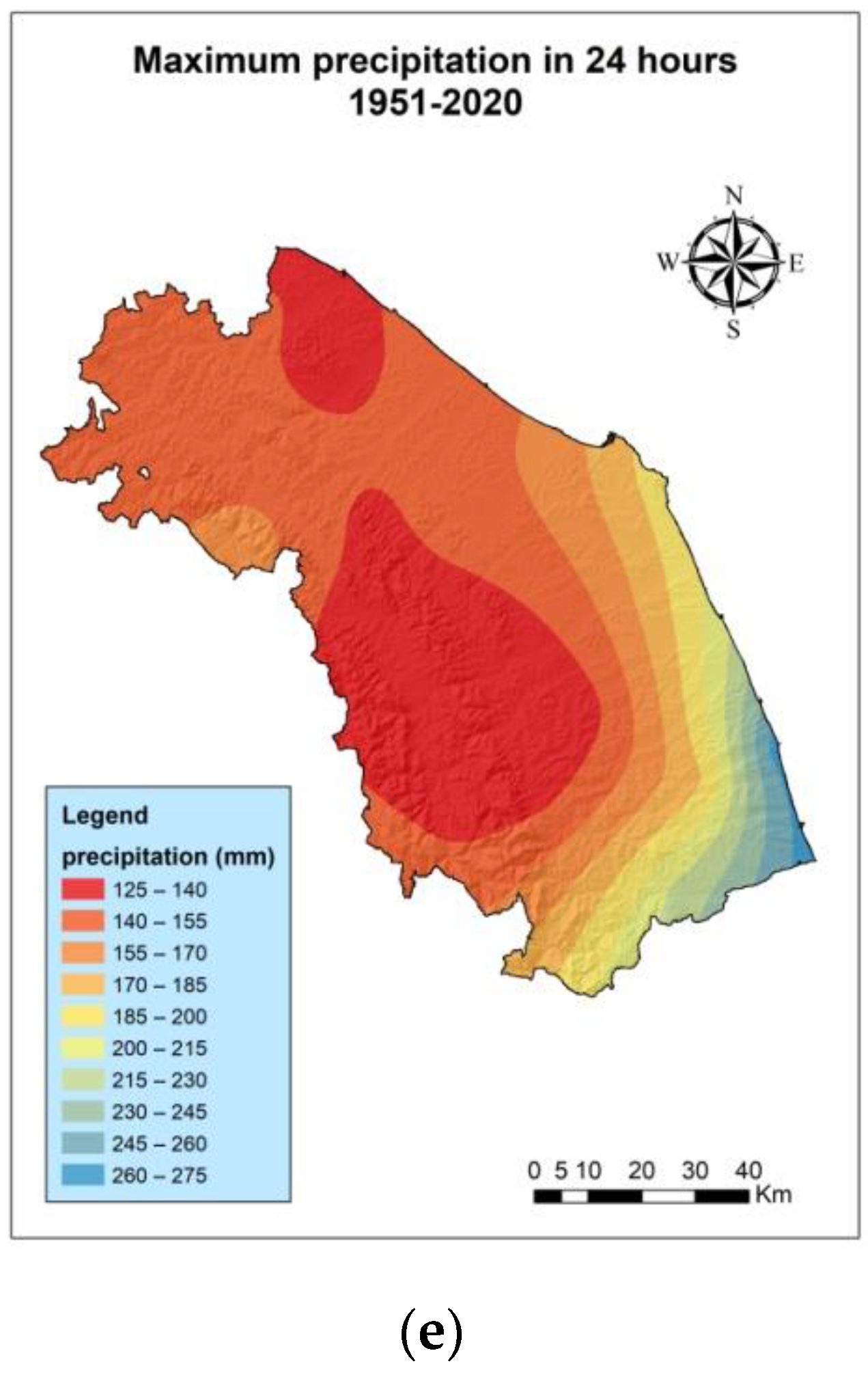
3.1. Analysis of Maximum Extreme Events for the Periods 1991–2020 and 1951–2020

The data collected for the individual weather stations over the periods 1991–2020 and 1951–2020 were plotted on the map with the correct coordinates and spatialised using the EBK method; the data chosen were the maximum precipitation data at 1, 3, 6, 12, 24 h. This procedure generated five maps of maximum precipitation events for each period, providing an overview, which is indispensable for comparison with return values in order to understand the possible underestimations in the prediction of extreme events with 100-year return times.

The interpolations of the extreme maximum rainfall at 1 and 3 h show modest rainfall peaks in the Apennine area, ranging from 50 mm for 1 h to 70 mm for 3 h; the central-southern area appears to have more rainfall than the others in the 1 h interval, about 58–60 mm, while for the 3 h, it reaches peaks of 70 mm. The area with the greatest peak of rainfall for both 1 h and 3 h appears to be the area to the northwest, approximately near Fonte Avellana and Monte Catria, with 62 mm of rain in 1 h and 90 mm of rain in 3 h (Figure 7a,b). In the 6, 12 and 24 h interpolations of extreme maximum rainfall, it can be seen that the highest values are to be found in the central-northern hinterland, as well as in the southern part of the region (Figure 7c–e). In particular, it is in the southern part of the area where the highest peaks were reached, with values between 200 and 240 mm in 24 h (Figure 7e).

Over the period 1951–2020, the relative spatial distribution of the areas with the most or least extreme precipitation events is almost homogeneous for all hours, except in the case of the 1 h map. In fact, the 1 h map of maximum precipitation events shows the highest values in a small patch of the coastal zone in the north-central part of the study area, while the northern part has the lowest values (Figure 8a). The other maps (Figure 8b–e), on the other hand, show higher values in the central-southern coastal area, while the extreme events with lower values are located in the Apennines and in the neighbouring valleys and hills.

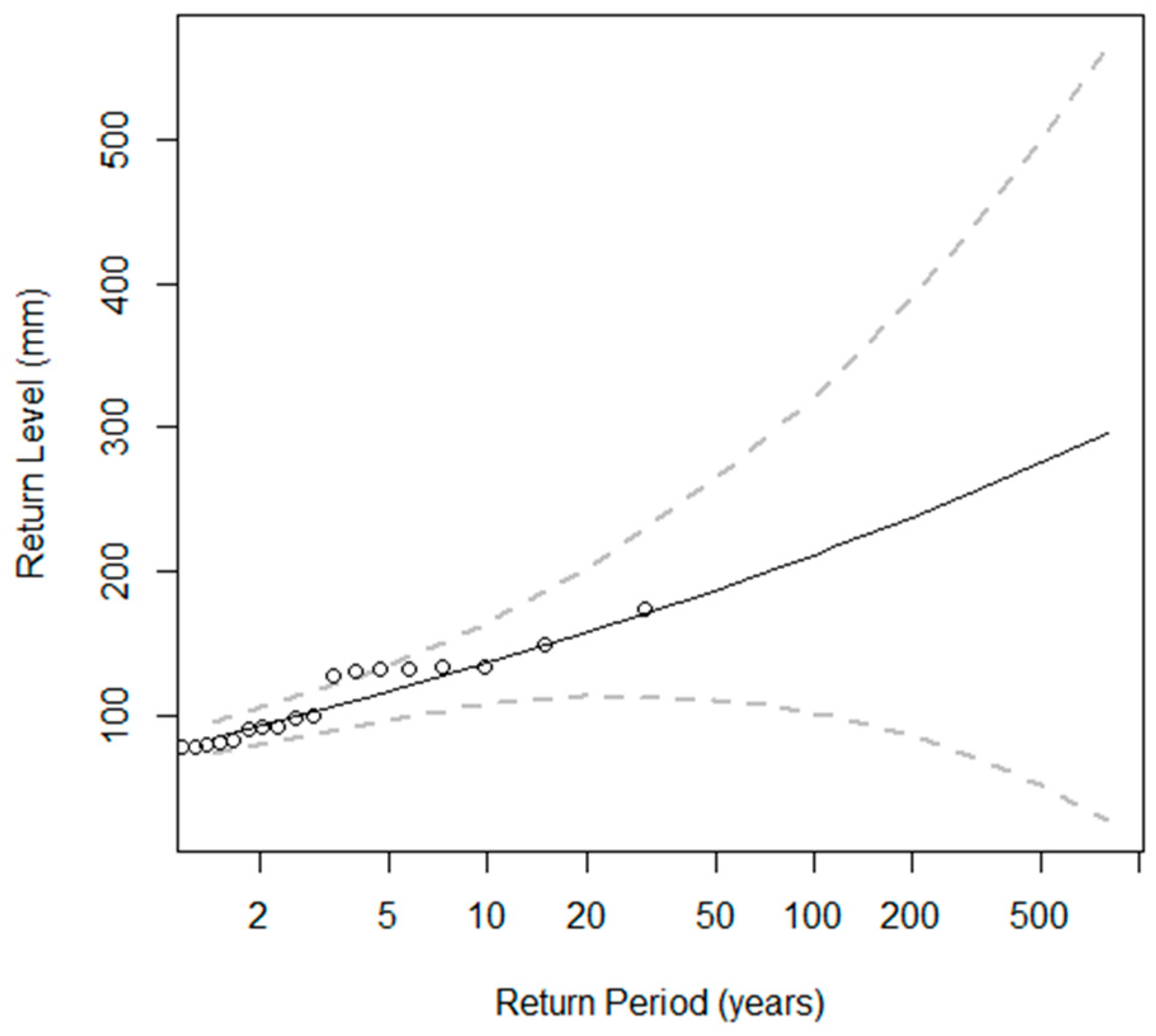
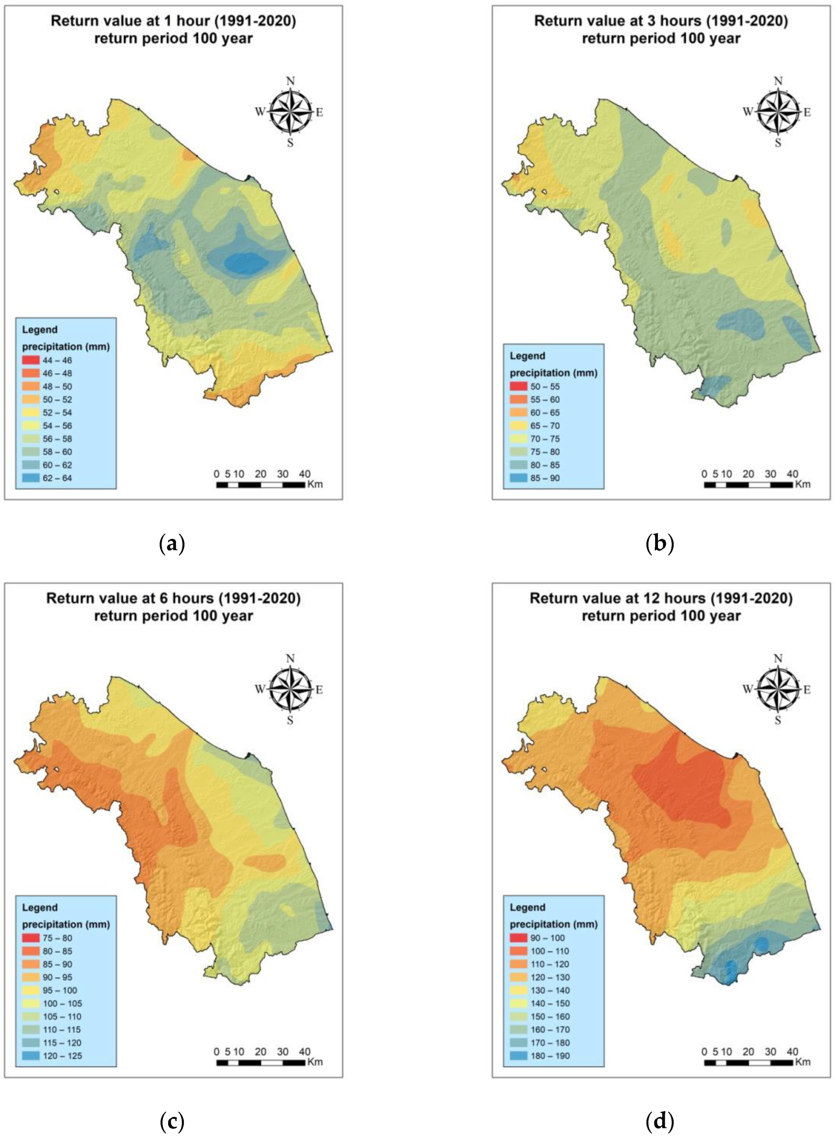
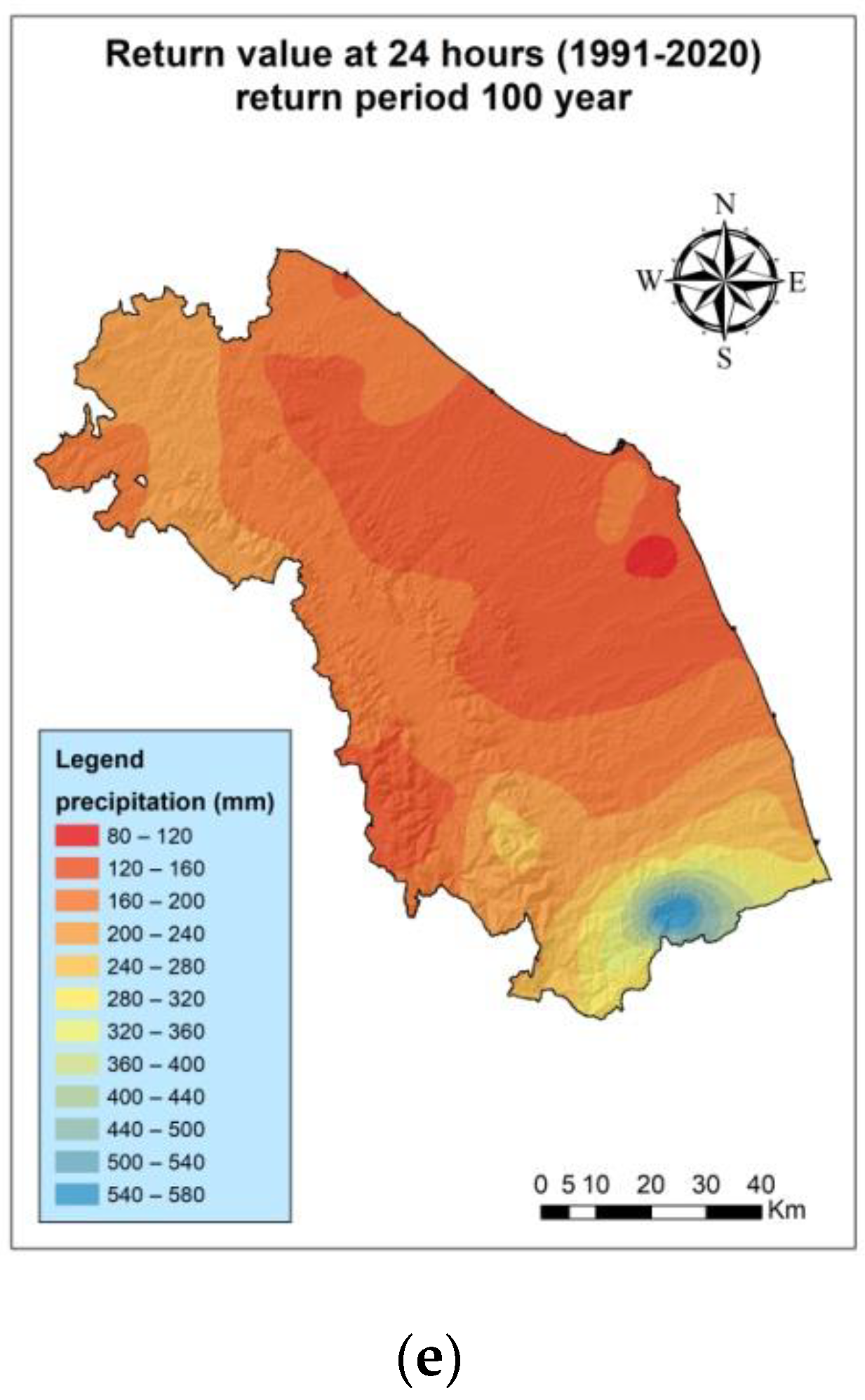
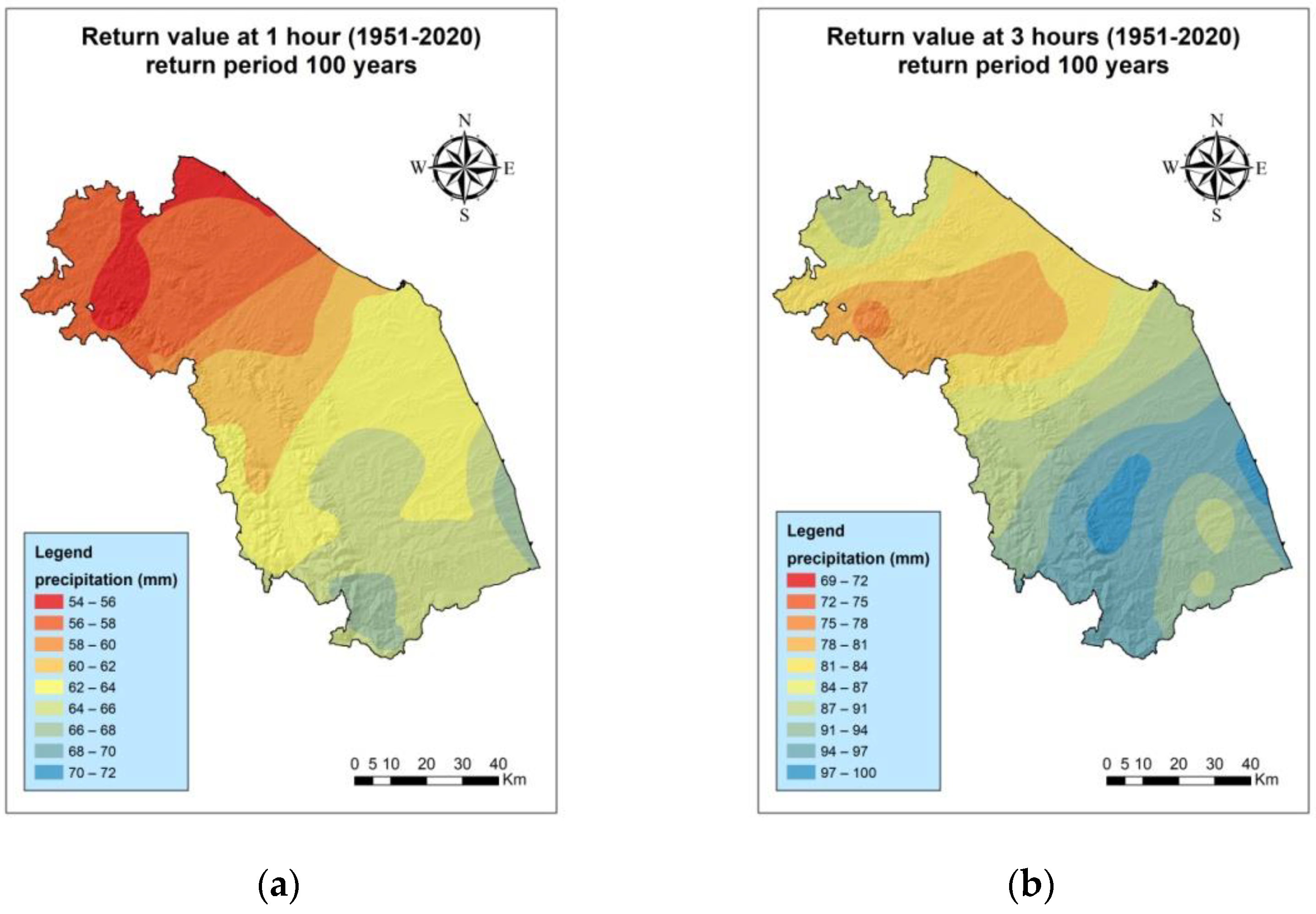
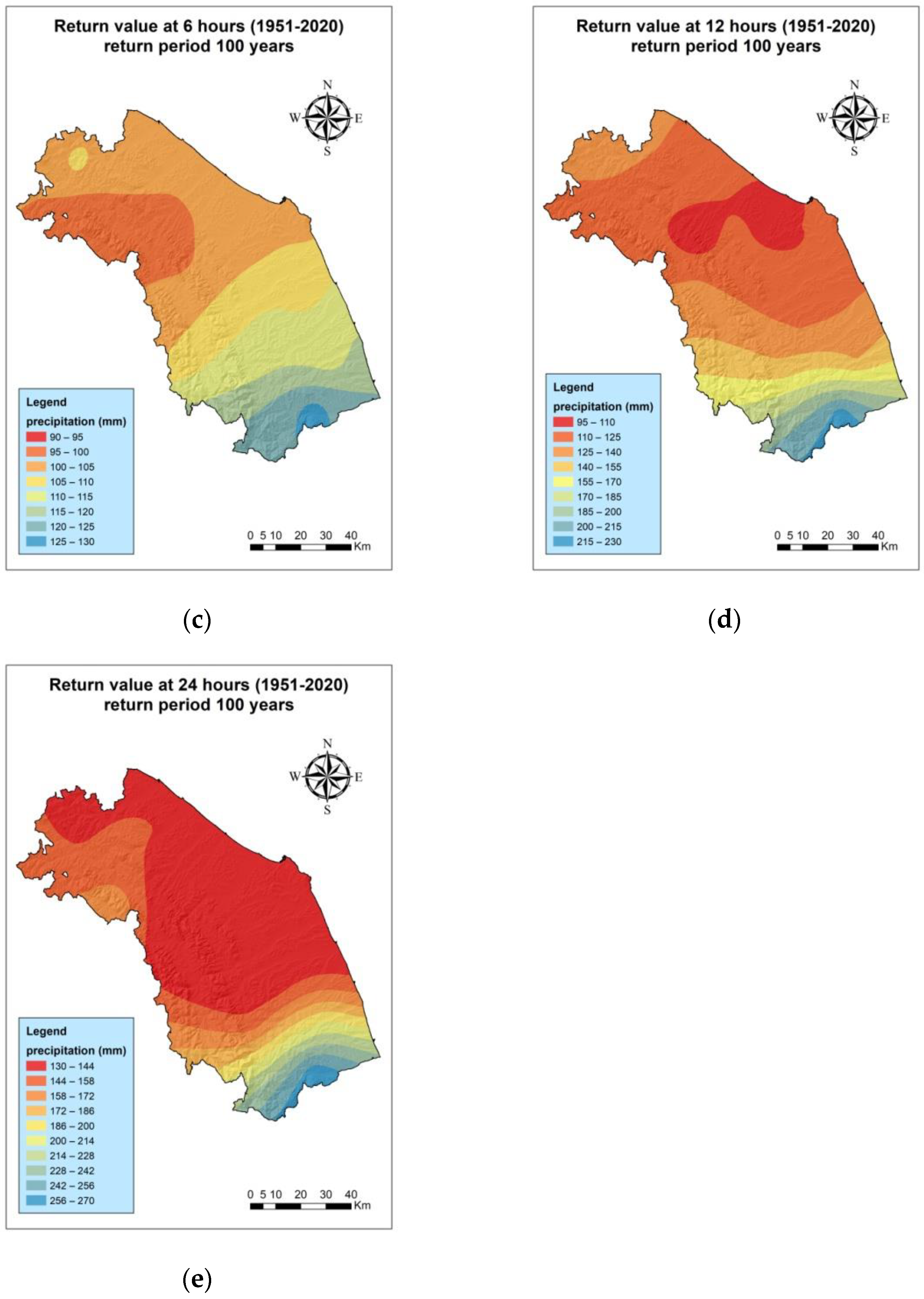
3.2. 100-Year Return Levels for the Periods 1991–2020 and 1951–2020

The 100-year return level was analysed for all periods (1951–2020 and 1991–2020) and all investigated time intervals (1, 3, 6, 12, 24), as well as for all available weather stations, of which there were 131 in total. The GEV block maxima methodology allowed the identification of the 100-year return level for the various stations, as shown in the graph in Figure 9.

The 100-year return level values obtained for the hours (1, 3, 6, 12, 24) were interpolated through ArcGis software using the EBK to obtain pluviometric probability maps for the Marche region from 1991 to 2020 (Figure 10).

The 1 h return level map (Figure 10a) shows that the highest values are found in the central part of the region, with the range of the highest values between 60 and 64 mm of rain. The 3 h return level map (Figure 10b) shows the highest values in the south, while the lowest values are found in the far north (70–80 mm). The 6 h return level map has higher values in the south, which are also common for the 12 h and 24 h intervals to various degrees (Figure 10c–e).

The same type of analysis was conducted for the interval 1951–2020, which revealed a smoother interpolated surface and also greater homogeneity between the various zones of the study area (Figure 11).

The 1 h and 3 h maps are similar, showing the same areas with the highest return levels, with the central-southern part of the region being more prone to the return of extreme rainfall. For the 1 h map, the return values are around 68 mm, while for the 3 h map, the values are around 100 mm. The 6, 12 and 24 h maps show the southern part of the study area as the area with the highest values. In contrast with the 1 h and 3 h maps, the values here are more localised in the far south (Figure 11a,b). The 6 h map assumes values around 128 mm as maximum return levels; the 12 h map values are around 200 mm, while the 24 h map values are 270 mm (Figure 11c–e).

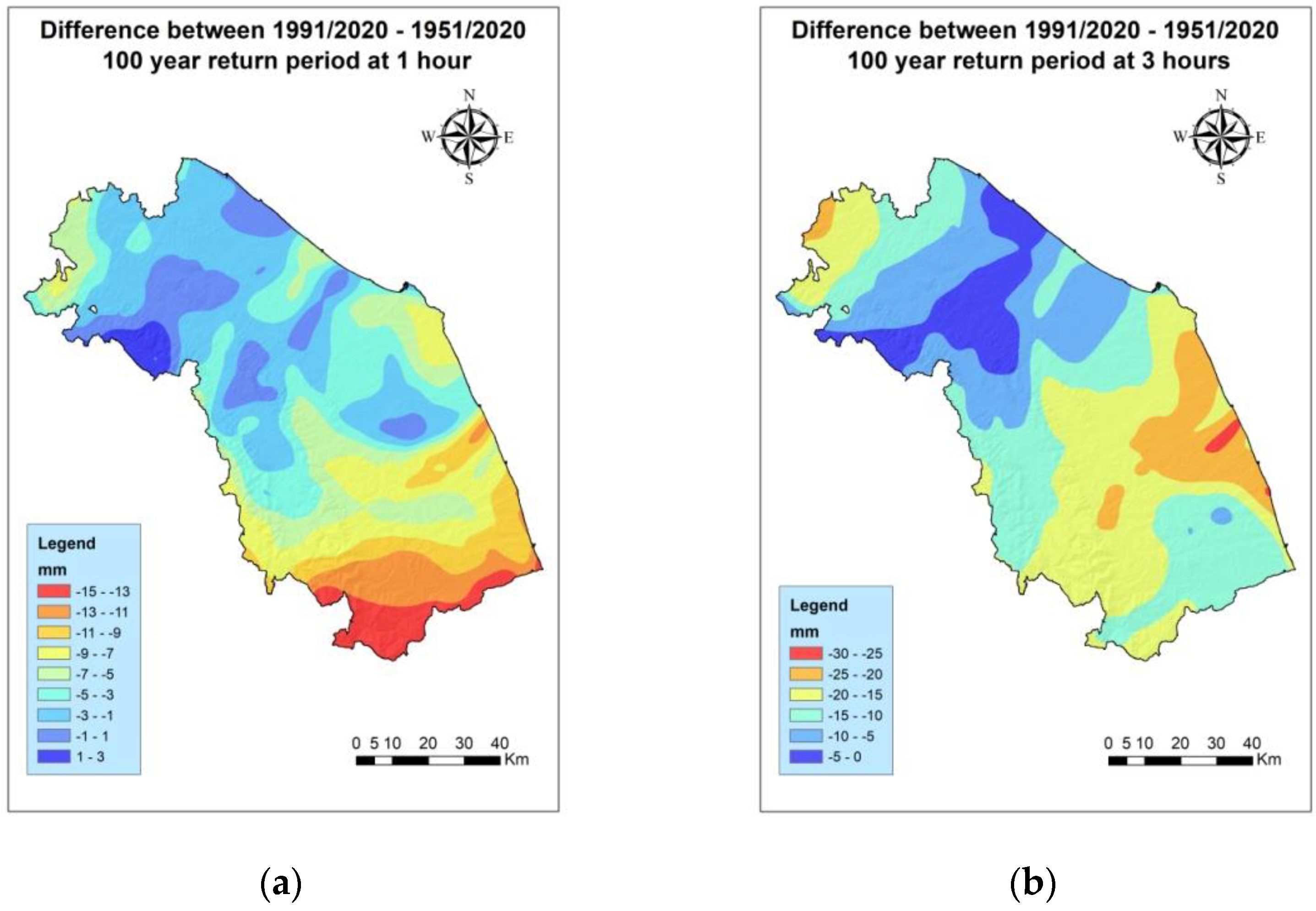
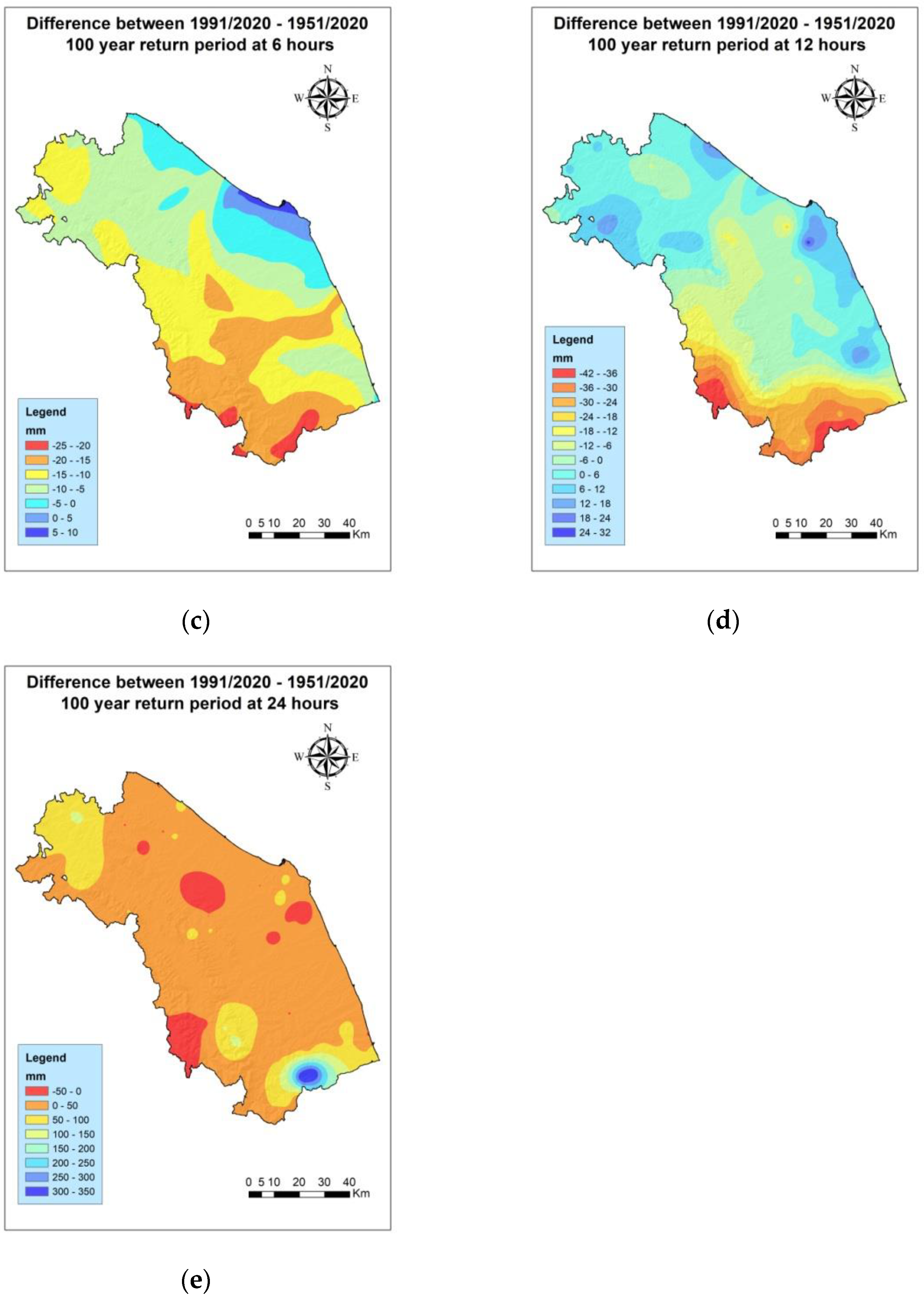
3.3. Analysis of the Differences between the Periods 1991–2020 and 1951–2020

The GIS software (ArcGis 10.8) makes it possible to perform operations between rasters, which are indispensable in some cases for assessing the spatial differences that may occur between two time series. In this case, using the maps in Figure 10 and Figure 11, the period 1991–2020 was subtracted from the period 1951–2020, resulting in an explanatory map of the differences in the return value calculated using a different time interval in the series.

The 1 h and 3 h maps have the only positive values located in a narrow area to the north, which runs from the Apennines to the coast, while negative values prevail for the rest of the study area, indicating that the longer time series leads to slightly higher 100-year return values than the 30-year period 1991–2020 (Figure 12a,b). The map of the differences between the 6 h periods also shows higher values for the period 1951–2020 spread over most of the area, with the exception of a small part of the north-central coast showing lower values, compared to the period 1991–2020 (Figure 12c). The trend in the study area is reversed in the comparison map between the two periods for both the 12 h and 24 h intervals, where it becomes evident that the 1991–2020 period results in higher return values than the 1951–2020 period everywhere, except in the extreme south of the study area. In addition, the values of some weather stations with complete or very few data gaps for both study periods 1951–2020 and 1991–2020 were compared in order to better understand the quantitative differences between the two intervals.

The same weather stations for both periods show different return values; in particular, the period 1991–2020 gives rise to consistently higher return values than the period 1951–2020 (

Table 2. Comparisons between the same active weather stations for the two periods studied (1951–2020 and 1991–2020). Code = unique code of each weather station, which can be found in the map in Figure 2 and Table 1; Period = period to which the data in the row refer; 1 h, 3 h, 6 h, 12 h, 24 h = values with 100-year return period.

Code	Period	1 h	3 h	6 h	12 h	24 h
10	1951–2020	53.6	72	78.8	95.5	125
10	1991–2020	128.3	163.2	172.5	176.2	184.1
39	1951–2020	63.3	88.8	100	131.8	141
39	1991–2020	115.4	119.6	122.5	133.8	159
52	1951–2020	54.7	75.7	96	101.3	124.6
52	1991–2020	106.2	110	120	126.6	148
83	1951–2020	75	104.5	119.2	142.8	165.4
83	1991–2020	90	115.2	122.2	159.3	170.8
110	1951–2020	75	110	114.3	141.6	150
110	1991–2020	81.2	145.8	223.5	258.8	263.1

).

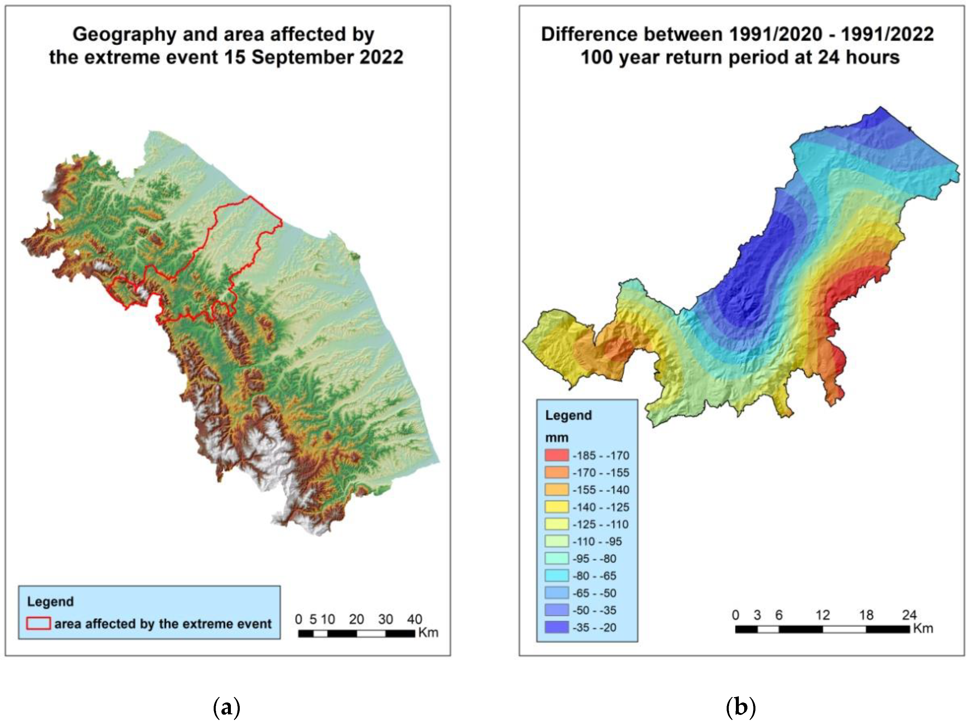
3.4. Effect of the Introduction of an Extreme Event on the 100-Year Return Value Evaluated over 24 h

On 15 September 2022, part of the study area was affected by an extreme rainfall event triggered by a V-shaped thunderstorm (Figure 13a). The flood triggered by the event caused 12 fatalities, 1 woman missing, 50 injured, 150 displaced persons and EUR 2 billion in damage. The difference was assessed by taking into account the reference period 1991–2020 and comparing it in the area where the extreme event was most intense with the period 1991–2022 by including the extreme event of 15 September 2022.

The difference between 1991–2020 and 1991–2022 in the reduced area where the extreme event was most intense is evident, with much higher return levels when considering the extreme event in the reference period, with values ranging from 30 to 180 mm more precipitation (Figure 13b).

4. Discussion

Two periods, 1991–2020 and 1951–2020, were analysed using all the meteorological stations available in the area in all the canonical time intervals indicated for defining extreme events. In the literature, most research on extreme events is carried out in hourly time intervals, whereas with regard to reference periods, there is a tendency to use methods of evaluating extreme events by entering as much data as available, i.e., the longest data set available [31,32,33]. Certainly, the use of long time series can be favourable in the absence of climate change, with stationary extreme events not influenced by trends, while in an opposite situation [34], it is necessary to assess whether it is really favourable for the prediction of expected extreme events or whether it is better to use shorter data intervals, which can take into account the more pronounced upward trends of recent years. The main aim of the present study was precisely to understand whether a shorter interval can lead to differences in the 100-year forecast by favouring return values, which are closer to those occurring. In this study, first, a GEV statistical analysis was performed for each weather station collected. Then, a spatial interpolation was carried out using EBK to obtain two rasters (one for each reference period) for each time interval 1, 3, 6, 12, 24; the subtraction between the rasters allowed the spatial understanding of the differences obtained in terms of the return levels for both periods. Very often in the literature, the subtraction between rasters created through the GEV methodology is performed in order to understand whether there is an increasing trend in the intensity of extreme events; however, there is no evidence of its use to verify the accuracy of the 100-year return value [35]. It is even argued in the literature that using series that are too short with respect to return time leads to unreliable and often non-predictive results [36]. Contrary to what has been reported in the literature so far, in this research, a certain underestimation of the return values was highlighted, especially for the longer period 1951–2020, in relation to events that already occurred, such as those in 2013 in the south of the region; in the Acquasanta Terme weather station, as much as 314 mm of precipitation fell in 24 h. In this zone, south of the study area, the period 1951–2020 predicts about 290 mm with a 100-year return time, while the period 1991–2020 predicts more than 600 mm, showing a greater sensitivity to extreme peaks in the series, which could, however, be appreciable in the context of an increasing trend of extreme events. This difference in the results between the investigated periods is also appreciable in relation to the extreme event of 2022, which reported values well above the forecasts for both periods analysed with the GEV method, although the shorter data series 1991–2020 showed higher values than the other series. In particular, for the period 1991–2020, values of between 150 and 210 mm were recorded in the area of the extreme event of 15 September 2022, while for the period 1951–2020, the 100-year return values were between 130 and 180 mm; the extreme precipitation event in question had values in the area of between 420 and 150 mm, so in some locations, there was twice as much rainfall as the 100-year return value, and even the 500-year return values in the area never exceeded 350 mm. Finally, a targeted analysis was also carried out of the area affected by the extreme event of 15 September 2015, and again, the shorter period showed results, which were higher and more in line with what had occurred, also showing how the addition of an extreme event of great intensity radically changed the results obtained from the GEV analysis. Thus, in addition to questioning the real usefulness of a longer time series in the context of climate change, one also questions the predictive capabilities of the GEV model, which was found to be rather inadequate for the predictive purposes for which it was used.

5. Conclusions

The study of extreme precipitation events is a very important topic because of the hydrogeological risks they can trigger. The scientific literature usually approaches this topic in a rather canonical manner by comparing different return value calculation methodologies, such as GDP and GEV; however, no attempt is made to assess the actual correctness of the method and also the influence, which the length of the time series has. This study shows that, in the case of a non-stationary time series, it is more appropriate to calculate the return value over a period of at least 30 years, as indicated by the World Meteorological Organisation (WMO), but not as long as possible, as is usually performed, precisely because it would tend to reduce the return value results. Furthermore, the problematic nature of the GEV method in correctly predicting the return value, even in the case of smaller time series, was highlighted, showing 100-year values, which are often lower than those that have already occurred or occurred just after the end of the reference period. It follows that, in the case of a climate change situation, such as the current one, the GEV methodology cannot be considered reliable for predicting extreme events, which may occur in the future. This obviously creates problems both for sizing the engineering works aimed at containing or mitigating the related hydrogeological risks and for the erroneous climate analysis. This study is a preliminary to a detailed sustainability study, as avoiding economic losses due to flood danger is increasingly crucial. The increase in the intensity of extreme events is a consequence of climate change, which is now evident, but a long-term forecast of the maximum intensity allows for countermeasures to be planned to improve the resilience of territories [37]. In addition, the spatial analysis performed in this study makes it possible to differentiate the areas at higher or lower risk from extreme events, laying the basis for the drafting of a reliable climate change adaptation plan.

References

1. Song, Y.; Achberger, C.; Linderholm, H.W. Rain-season trends in precipitation and their effect in different climate regions of China during 1961–2008. Environ. Res. Lett. 2011, 6, 034025. [Google Scholar] [CrossRef] [Green Version]
2. Letcher, T. Climate Change: Observed Impacts on Planet Earth; Elsevier: Amsterdam, The Netherland, 2021. [Google Scholar]
3. Jubb, I.; Canadell, P.; Dix, M. Representative Concentration Pathways (RCPs); Australian Government, Department of the Environment: Canberra, Australia, 2013. [Google Scholar]
4. Guhathakurta, P.; Sreejith, O.P.; Menon, P.A. Impact of climate change on extreme rainfall events and flood risk in India. J. Earth Syst. Sci. 2011, 120, 359–373. [Google Scholar] [CrossRef]
5. Huber, D.B.; Mechem, D.B.; Brunsell, N.A. The effects of Great Plains irrigation on the surface energy balance, regional circulation, and precipitation. Climate 2014, 2, 103–128. [Google Scholar] [CrossRef] [Green Version]
6. Schmith, T.; Thejll, P.; Berg, P.; Boberg, F.; Christensen, O.B.; Christiansen, B.; Christensen, J.H.; Madsen, M.S.; Steger, C. Identifying robust bias adjustment methods for European extreme precipitation in a multi-model pseudo-reality setting. Hydrol. Earth Syst. Sci. 2021, 25, 273–290. [Google Scholar] [CrossRef]
7. Rootzén, H.; Katz, R.W. Design life level: Quantifying risk in a changing climate. Water Resour. Res. 2013, 49, 5964–5972. [Google Scholar] [CrossRef] [Green Version]
8. Zheng, L.; Ismail, K.; Meng, X. Freeway safety estimation using extreme value theory approaches: A comparative study. Accid. Anal. Prev. 2014, 62, 32–41. [Google Scholar] [CrossRef]
9. Malevergne, Y.; Pisarenko, V.; Sornette, D. On the power of generalized extreme value (GEV) and generalized Pareto distribution (GPD) estimators for empirical distributions of stock returns. Appl. Financ. Econ. 2006, 16, 271–289. [Google Scholar] [CrossRef]
10. Blanchet, J.; Ceresetti, D.; Molinié, G.; Creutin, J.D. A regional GEV scale-invariant framework for Intensity–Duration–Frequency analysis. J. Hydrol. 2016, 540, 82–95. [Google Scholar] [CrossRef]
11. Kim, H.; Kim, S.; Shin, H.; Heo, J.H. Appropriate model selection methods for nonstationary generalized extreme value models. J. Hydrol. 2017, 547, 557–574. [Google Scholar] [CrossRef]
12. Brabson, B.B.; Palutikof, J.P. Tests of the generalized Pareto distribution for predicting extreme wind speeds. JAMC 2000, 39, 1627–1640. [Google Scholar] [CrossRef]
13. Wang, J.; Han, Y.; Stein, M.L.; Kotamarthi, V.R.; Huang, W.K. Evaluation of dynamically downscaled extreme temperature using a spatially-aggregated generalized extreme value (GEV) model. Clim. Dyn. 2016, 47, 2833–2849. [Google Scholar] [CrossRef]
14. Alentorn, A.; Markose, S. Generalized extreme value distribution and extreme economic value at risk (EE-VaR). In Computational Methods in Financial Engineering: Essays in Honour of Manfred Gilli; Springer: Berlin/Heidelberg, Germany, 2008; pp. 47–71. [Google Scholar]
15. Chen, B.Y.; Zhang, K.Y.; Wang, L.P.; Jiang, S.; Liu, G.L. Generalized extreme value-pareto distribution function and its applications in ocean engineering. China Ocean Eng. 2019, 33, 127–136. [Google Scholar] [CrossRef]
16. Carney, M.C. Bias correction to gev shape parameters used to predict precipitation extremes. J. Hydrol. Eng. 2016, 21, 04016035. [Google Scholar] [CrossRef]
17. Gentilucci, M.; Barbieri, M.; Pambianchi, G. Reliability of the IMERG product through reference rain gauges in Central Italy. Atmos. Res. 2022, 278, 106340. [Google Scholar] [CrossRef]
18. DeGaetano, A.T. Time-dependent changes in extreme-precipitation return-period amounts in the continental United States. JAMC 2009, 48, 2086–2099. [Google Scholar] [CrossRef] [Green Version]
19. Koutsoyiannis, D.; Baloutsos, G. Analysis of a long record of annual maximum rainfall in Athens, Greece, and design rainfall inferences. Nat. Hazards 2000, 22, 29–48. [Google Scholar] [CrossRef]
20. Gentilucci, M.; Barbieri, M.; D’Aprile, F.; Zardi, D. Analysis of extreme precipitation indices in the Marche region (central Italy), combined with the assessment of energy implications and hydrogeological risk. Energy Rep. 2020, 6, 804–810. [Google Scholar] [CrossRef]
21. Antonetti, G.; Gentilucci, M.; Aringoli, D.; Pambianchi, G. Analysis of landslide Susceptibility and Tree Felling Due to an Extreme Event at Mid-Latitudes: Case Study of Storm Vaia, Italy. Land 2022, 11, 1808. [Google Scholar] [CrossRef]
22. Gentilucci, M.; Djouohou, S.I.; Barbieri, M.; Hamed, Y.; Pambianchi, G. Trend Analysis of Streamflows in Relation to Precipitation: A Case Study in Central Italy. Water 2023, 15, 1586. [Google Scholar] [CrossRef]
23. Webster, P.J.; Jian, J. Environmental prediction, risk assessment and extreme events: Adaptation strategies for the developing world. Philos. Trans. R. Soc. A Math. Phys. Eng. Sci. 2011, 369, 4768–4797. [Google Scholar] [CrossRef]
24. Bartolini, G.; Grifoni, D.; Torrigiani, T.; Vallorani, R.; Meneguzzo, F.; Gozzini, B. Precipitation changes from two long-term hourly datasets in Tuscany, Italy. Int. J. Climatol. 2014, 34, 3977–3985. [Google Scholar] [CrossRef]
25. Gentilucci, M.; Pambianchi, G. Prediction of Snowmelt Days Using Binary Logistic Regression in the Umbria-Marche Apennines (Central Italy). Water 2022, 14, 1495. [Google Scholar] [CrossRef]
26. Gilleland, E.; Katz, R.W. extRemes 2.0: An Extreme Value Analysis Package in R. J. Stat. Soft. 2016, 72, 1–39. [Google Scholar] [CrossRef] [Green Version]
27. Aggag, A.M.; Alharbi, A. Spatial Analysis of Soil Properties and Site-Specific Management Zone Delineation for the South Hail Region, Saudi Arabia. Sustainability 2022, 14, 16209. [Google Scholar] [CrossRef]
28. Krivoruchko, K.; Gribov, A. Evaluation of empirical Bayesian kriging. Spat. Stat. 2019, 32, 100368. [Google Scholar] [CrossRef]
29. Embrechts, P.; Resnick, S.I.; Samorodnitsky, G. Extreme value theory as a risk management tool. N. Am. Actuar. J. 1999, 3, 30–41. [Google Scholar] [CrossRef]
30. Gilleland, E.; Katz, R. In2extRemes: Into the R Package ExtRemes. Extreme Value Analysis for Weather and Climate Applications, 2016 (No. NCAR/TN-523+STR). Available online: https://opensky.ucar.edu/islandora/object/technotes:534 (accessed on 2 February 2023).
31. Crisci, A.; Gozzini, B.; Meneguzzo, F.; Pagliara, S.; Maracchi, G. Extreme rainfall in a changing climate: Regional analysis and hydrological implications in Tuscany. Hydrol. Process. 2002, 16, 1261–1274. [Google Scholar] [CrossRef]
32. Yilmaz, A.G.; Perera, B.J.C. Extreme rainfall nonstationarity investigation and intensity–frequency–duration relationship. J. Hydrol. Eng. 2014, 19, 1160–1172. [Google Scholar] [CrossRef] [Green Version]
33. Fiorillo, F.; Diodato, N.; Meo, M. Reconstruction of a storm map and new approach in the definition of categories of the extreme rainfall, northeastern Sicily. Water 2016, 8, 330. [Google Scholar] [CrossRef] [Green Version]
34. Persiano, S.; Ferri, E.; Antolini, G.; Domeneghetti, A.; Pavan, V.; Castellarin, A. Changes in seasonality and magnitude of sub-daily rainfall extremes in Emilia-Romagna (Italy) and potential influence on regional rainfall frequency estimation. J. Hydrol. Reg. Stud. 2020, 32, 100751. [Google Scholar] [CrossRef]
35. Rahmani, V.; Hutchinson, S.L.; Hutchinson, J.S.; Anandhi, A. Extreme daily rainfall event distribution patterns in Kansas. J. Hydrol. Eng. 2014, 19, 707–716. [Google Scholar] [CrossRef]
36. Huang, W.K.; Stein, M.L.; McInerney, D.J.; Sun, S.; Moyer, E.J. Estimating changes in temperature extremes from millennial-scale climate simulations using generalized extreme value (GEV) distributions. Adv. Stat. Climatol. Meteorol. Oceanogr. 2016, 2, 79–103. [Google Scholar] [CrossRef] [Green Version]
37. Merz, B.; Aerts JC, J.H.; Arnbjerg-Nielsen, K.; Baldi, M.; Becker, A.; Bichet, A.; Blöschl, G.; Bouwer, L.M.; Brauer, A.; Cioffi, F.; et al. Floods and climate: Emerging perspectives for flood risk assessment and management. Nat. Hazards Earth Syst. Sci. 2014, 14, 1921–1942. [Google Scholar] [CrossRef] [Green Version]
Figure 1. Geographic map of the study area.
Sustainability 15 11656 g001
Figure 2. Rain gauges in the study area identified with a code number traceable in Table 1 and a red dot.
Sustainability 15 11656 g002
Figure 3. Research flow chart.
Sustainability 15 11656 g003
Figure 4. Distributions of Gumbel, Frechet and Weibull [29].
Sustainability 15 11656 g004
Figure 5. Graphs resulting from the GEV analysis performed with the in2extEemes package: model quantiles (the dots indicate the data, if they follow the line these quantiles are normally distributed), empirical quantiles (qq-plot for randomly generated data from the fitted GEV df against the empirical data quantiles along with 95% confidence bands identified by two dotted curves, a 1-1 line and a fitted regression line), frequency histogram (empirical density of observed annual maxima, solid black line, with fitted GEV df density, dashed dark blue line), return level plot (return level plot in a log scale, with 95% normal approximation point-wise confidence intervals, identified by two dotted curves) [30].
Sustainability 15 11656 g005
Figure 6. Example of nomenclature and analysis of spatial correlation in a semivariogram.
Sustainability 15 11656 g006
Figure 7. Maximum extreme precipitation from 1991 to 2020 at 1 h (a), at 3 h (b), at 6 h (c), at 12 h (d), at 24 h (e).
Sustainability 15 11656 g007aSustainability 15 11656 g007b
Figure 8. Maximum extreme precipitation from 1951 to 2020 at 1 h (a), at 3 h (b), at 6 h (c), at 12 h (d), at 24 h (e).
Sustainability 15 11656 g008aSustainability 15 11656 g008b
Figure 9. Example of the return level graph for the Cantiano weather station, return level plot (log scale) with 95% normal approximation point-wise confidence intervals, identified by two dotted curves, measured data are summarised by the dots.
Sustainability 15 11656 g009
Figure 10. Interpolation for the period 1991–2020 of the 100-year return level at the following intervals: 1 h (a), 3 h (b), 6 h (c), 12 h (d), 24 h (e).
Sustainability 15 11656 g010aSustainability 15 11656 g010b
Figure 11. Interpolation for the period 1951–2020 of the 100-year return level at the following intervals: 1 h (a), 3 h (b), 6 h (c), 12 h (d), 24 h (e).
Sustainability 15 11656 g011aSustainability 15 11656 g011b
Figure 12. Subtraction between the return value calculated with the time series 1991–2020 and that calculated with the time series 1951–2020: 1 h (a), 3 h (b), 6 h (c), 12 h (d), 24 h (e).
Sustainability 15 11656 g012aSustainability 15 11656 g012b
Figure 13. (a) map of the Marche region, the area studied for the extreme event of September 2022 is shown in red; (b) maps of the variation in return level between the periods 1991/2020 and 1991/2022 at 24 h.
Sustainability 15 11656 g013