
Temporal and Spatial Distribution of Ozone and Its Influencing Factors in China
School of Management, China University of Mining and Technology, Beijing 100083, China
*
Author to whom correspondence should be addressed.
Sustainability 2023, 15(13), 10042; https://doi.org/10.3390/su151310042
Submission received: 12 May 2023
/
Revised: 18 June 2023
/
Accepted: 19 June 2023
/
Published: 25 June 2023
Abstract
:Tropospheric ozone (O3) pollution has emerged as a significant concern, as it can adversely influence human health, daily activities, and the surrounding environment(The following tropospheric O3 is referred to as O3). Research on the societal contribution to O3 primarily concentrates on the generation mechanisms and chemical processes, with limited studies examining the influence of social and economic activities on O3 at a national scale. In this investigation, spatial econometric models, random forest models, and geographically weighted regression (GWR) were adopted for assessing the effects of meteorological, natural, and socioeconomic factors on O3 concentration throughout the country. The spatial error model (SEM) revealed that precipitation, temperature, wind direction, per capita GDP, RD project funding, and SO2 were the primary factors influencing O3 concentration in China, among which precipitation had the strongest effect on O3, followed by temperature and SO2. Subsequently, the GWR model was utilized to demonstrate the regional differences in the impacts of precipitation, NOx, secondary industry proportion, and electricity consumption. In central and western regions, such as Jiangxi, Guangxi, and Guizhou, precipitation, NOx, and power consumption were the leading factors contributing to severe O3 pollution. The secondary industry proportion substantially affected O3 pollution in the Beijing-Tianjin-Hebei region, indicating that this sector played a crucial role in the region’s economic growth and contributed to elevated O3 concentrations. Meteorological, natural, and socioeconomic factors exhibited a lesser influence on O3 pollution in most eastern regions compared to central and western regions. This study’s findings identified the primary contributors to O3 pollution and provided a scientific basis for developing strategies to mitigate its impact.
1. Introduction
In recent years, due to escalating urban development and global warming [1], O3 has become a significant pollutant impacting air quality in China. As outlined in the Strengthening of the Collaborative Control of PM2.5 and Ozone and Deepening the Battle to Protect Blue Sky [2], from 2021 onwards, efforts to address the weak links in ozone pollution prevention and control must be intensified, aiming to effectively control the rise in ozone concentration by 2025. Numerous studies have shown that exceedingly high concentrations of O3 can diminish agricultural productivity and quality [3] and negatively affect food security [4]. Furthermore, elevated O3 concentrations can cause respiratory diseases and lung function [5] impairment, thereby posing risks to human health [6,7]. In 2013, due to overexposure to O3, 16,000 premature deaths occurred in 28 EU countries, equivalent to 192,000 years of life lost [8]. Following the implementation of the Action Plan of Air Pollution Prevention and Control by the State Council on 10 September 2013, China saw promising results in air pollution prevention and control [9]. Between 2015 and 2020, the concentration of PM2.5 in urban agglomerations significantly decreased [10]; however, O3 concentrations increased. Ozone primarily forms in cities through the reaction of nitrogen oxides (NOx), volatile organic compounds (VOCs), carbon monoxide (CO), and other precursors in the presence of light [11], with these substances consistently affected by human activities and industrial emissions [12,13]. Given the harmful nature of O3 pollution, it becomes crucial to identify the key factors contributing to O3 generation in order to mitigate its detrimental effects on humans and crops.
The investigation into the causes of air pollution, particularly the socioeconomic factors related to PM2.5 and SO2, has garnered increasing attention from researchers. Population density, industrialization level, and economic development are the primary factors influencing PM2.5 [14,15,16]. The impact of these factors also exhibits spatial differentiation at the prefecture-level city scale [17]. Chen et al. (2018) further explored the correlation between energy consumption, energy intensity, and PM2.5 concentration [18]. They discovered that, in the short term, all countries except those with low incomes could reduce PM2.5 concentration by increasing energy intensity. In China and its central and eastern regions, the association between PM2.5 concentration and urbanization followed an inverted U-shaped EKC model, while in the developed eastern regions, it adhered to an N-shaped EKC model [19]. These findings suggest that PM2.5 is significantly influenced by geospatial attributes and regional economic correlations in China [20]. In addition to PM2.5, research has also examined SO2 pollution. For instance, Jiang et al. (2020) analyzed the social and economic factors influencing SO2 pollution in 270 prefecture-level Chinese cities from 2005 to 2016 [21]. They found that SO2 pollution exhibited a gradual decline, indicating an overall improvement in China’s environmental quality. Although numerous studies have identified factors influencing PM2.5, SO2, and NO2, comprehensive and systematic analyses of O3’s influencing factors remain scarce.
Numerous studies have concentrated on examining the impact of PM2.5 and SO2 in relation to socioeconomic factors; however, similar research on O3 is scarce. Near-surface O3 is a common gaseous pollutant in the fundamental monitoring project of urban environmental air pollutants [22], and as such, it is influenced by social and economic factors. Gong et al. [23] explored the factors affecting O3 concentration changes in 96 urban areas within the Yangtze River Economic Belt from 2013 to 2020, identifying the GDP proportion of the secondary industry as the most significant factor influencing surface ozone concentration. Nonetheless, this study only considered regional data and did not examine changes on a national scale. This issue was addressed by Liu et al. [24], who discovered that O3 concentrations at a national level are influenced by both natural and human factors, with temperature, NOx, and VOCs being the key elements influencing O3 emissions. Yang et al. [25] analyzed O3 pollution in 338 Chinese cities over an extended period and observed that O3 concentrations in eastern China were generally higher than those in western China, with the most severe pollution occurring in the North, East, and Central regions. In addition, the relationship between COVID-19 and air pollution parameters demonstrated that people living in the epicentre of the outbreak were exposed to lower levels of O3 pollution due to geographical lockdowns [26]. Qi et al. [27] investigated the effect of lockdown during COVID-19 on surface ozone in Dongguan, an industrial city in southern China, and observed from long-term measurements in Dongguan that the ratio of daily Ox (O3 + NO2) enhancement to solar radiation during lockdown was smaller, suggesting that a significant weakening of photochemistry during the lockdown successfully reduces local ozone production. However, these studies only took into account meteorological and natural factors, neglecting the effect of socioeconomic factors on O3 concentrations. Social and economic factors indeed have a strong influence on O3 concentrations, as Yang et al. [28] found that changes in ozone concentrations are affected by human activities including industrialization, urbanization, and economic development. Despite this, these studies only considered the influence of socioeconomic factors on O3, with limited research examining the combined effects of meteorological factors, natural factors, and socioeconomic factors on O3. Consequently, in this study, we provide a comprehensive overview of O3 research that investigates the interplay of meteorological, natural, and socioeconomic factors across different provinces in China. Our findings may offer guidance and recommendations for the coordinated enhancement of the economic environment in various Chinese provinces.
To address these issues, we analyzed the effects of meteorological factors, natural factors, and socioeconomic factors on O3 in China on both national and provincial scales using the geographically weighted regression model (GWR) and spatial econometrics model, with 31 Chinese provinces from 2015 to 2020 as case studies. First, we examined the overall temporal change of O3 in the country, identified the temporal and spatial characteristics of O3 concentrations in different regions, and analyzed the concentration characteristics of O3 at the national level using the Mohn index. Second, employing the SLM and SEM, we investigated the linear global correlation between meteorological factors, natural factors, socioeconomic factors, and O3 concentrations as a whole, and subsequently, the random forest model was utilized to study the nonlinear relationships between variables. Third, we applied the GWR model to quantitatively determine the impact of spatiotemporal variation in the influencing factors on O3 pollution across various regions. Ultimately, we provided constructive guidance and suggestions for preventing and controlling O3 pollution in China.
2. Methodology and Data Sources
2.1. Data
The present study utilized the O3 concentration data from the ecological environment website of China (http://beijingair.sinaapp.com/, accessed on 3 December 2022) to assess air quality. To calculate the effective values and urban average daily concentration and establish evaluation standards, the Ambient Air Quality Standards (GB3095–2012) [29], Technical Specifications for Assessment of Ambient Air Quality (Trial) (HJ663–2013) [30] were consulted. O3 concentrations were collected from the website of the Ministry of Ecology and Environment of China, and the results were described as the actual ozone concentrations in the study area To ensure the validity of the O3 data, values with hourly O3 concentration ≤10 µg/m3 and missing values were eliminated from the original dataset. For the calculation of the daily mean value, if the monitoring point lacked test data for less than 16 h, the data for that day were considered invalid and discarded. To calculate the monthly mean value, if the monitoring point’s data for the current month was less than the average value of the maximum 8 h for 20 O3 days, the data for that month was considered invalid and removed. The method was to filter the data in Python, filtered out the elements that did not match the conditions, and returned an iterator object to convert it to a list. The reason for eliminating invalid data was that if the monitored data in one day or one month were too small, they would cause relatively large errors, which would affect the model effect. The reliability of the data was tested to confirm their credibility. The meteorological data applied in the present study included surface climatological data for China from the National Meteorological Information Center of China Meteorological Administration (http://data.cma.cn/, accessed on 12 December 2022). This dataset contained daily data for various parameters, including the average temperature, precipitation, wind speed, wind direction, and boundary layer height, for 367 Chinese cities from 2015 to 2020. The dataset adhered to the Meteorological Data Classification and Coding criteria, and the original data files underwent strict quality control and examination.
The statistics on socioeconomic and natural factors for each province during 2015–2020 were acquired from the China Statistical Information Network (http://data.stats.gov.cn/, accessed on 20 December 2022) and the China Statistical Yearbook (http://www.stats.gov.cn, accessed on 28 December 2022). The data primarily comprised information on per capita GDP (ten thousand yuan), the proportion of secondary industry (%), population (ten thousand people), electricity consumption (hundred million kilowatt hours), forest stock (ten thousand cubic meters), forest coverage rate (%), R&D project expenditure (ten thousand yuan), NOx (ten thousand tons), and SO2 (ten thousand tons). A literature review informed the selection of these indicators, which previous studies deemed as critical factors impacting O3 levels. For instance, per capita GDP is an essential indicator of the economic scale, and the secondary industry, with petroleum and chemical industries as its mainstays, can emit substantial amounts of atmospheric pollutants (including O3 precursors). Consequently, the economic scale may be the primary driver of increasing O3 column concentration [31]. In densely populated areas, O3 pollution levels are indirectly affected by VOCs, CO, NOx, and other precursors produced by human activities [32]. Numerous VOCs and BVOCs emitted by plants are significant photochemicals that participate in ozone formation [33,34]. NOx, as an O3 precursor, generates ozone through photochemical reactions under specific conditions, thereby increasing ozone concentration and exacerbating ozone pollution [35]. Moreover, O3 concentration is influenced by non-uniform chemical reactions occurring on particle surfaces, and an increase in particles, such as SO2, can diminish atmospheric radiation. This reduction may subsequently decrease ozone levels by eliminating ultraviolet rays [35].
2.2. Spatial Autocorrelation Test
Global autocorrelation is employed to describe the spatial clustering of O3 concentration within a region. In the present study, the spatial correlation of O3 concentration at the national scale is examined empirically using the Global Moran’s I index. The calculation of Moran’s I was as follows:
Here, I indicates the global Mohn index, indicates the total number of cities; and indicate the observed O3 pollution values of the and cities, respectively; refers to the average O3 concentration values of cities; indicates the spatial weight matrix element, whose values are 1 or 0, indicating adjacent or non-adjacent cities, respectively. Moran’s I has a value that fluctuates between −1 and 1. With the value being closer to −1, the spatial units with different attributes are more concentrated. Conversely, when the value is closer to 1, the spatial units with similar attributes are more concentrated.
The cold spots and hot spots of O3 concentration at various spatial locations in the region were identified using the Local Moran’s I index. The index can be calculated with the following formula:
Here, I indicates the local Mohn index, indicates the total number of cities, indicates the number of adjacent cities, and indicate the observed O3 pollution values of each province, is the average O3 concentration of cities, and suggests the spatial weight matrix element. On a small scale, the local Moran’s I approach is applied to describe the relationship between one site and its neighbors. The normalized O3 concentration of one site and adjacent sites are represented by the local Moran index, and their correlation can be seen on a scatter plot [36]. There are four local autocorrelation spatial association patterns, which include “high–high” aggregation (high-concentration city surrounded by high-concentration city), “high–low” aggregation (high-concentration city surrounded by low-concentration city), “low–low” aggregation (low-concentration city surrounded by low-concentration city), and “low–high” aggregation (low-concentration city surrounded by high-concentration city), and “not significant” indicates the specific spatial location of agglomeration. HH (LL) represented the proximity of the region to the same observed value attributes of the agglomeration city, i.e., the agglomeration of a low-value area and a low-value area, as well as the agglomeration of two high-value areas. HL (LH) represented the local spatial agglomeration characteristics of regions with opposite observed values.
2.3. Spatial Econometric Models
When addressing economic problems that involve spatial attributes, traditional econometric models tend to ignore the spatial correlation between research units and variables, leading to deviations in model findings and violating the classical least square method’s prerequisite. Therefore, it is essential to establish a spatial econometric regression model for data processing [37]. The spatial econometric model, which considers spatial effects and is suitable for sectional data, is a spatial constant coefficient regression model. There are various spatial econometric models, of which the spatial lag model (SLM) and the spatial error model (SEM) are widely used.
The spatial lag model (SLM) incorporates the lag variable, considering the time series, and the spatial lag by considering the impact of the surrounding area on the study area. It is an autoregressive model that considers spatial variables and is sometimes referred to as a spatial autoregressive model. The SLM is expressed as follows:
Here, represents the explained variable matrix, represents the explained variable matrix, represents constant, represents the space effect coefficient, represents the parameter vector, represents the space matrix, and stands for the random error term.
The spatial error model (SEM) primarily captures the interactive relationship of explained variables, considering the system effect by setting the hysteresis term of the disturbance term [38]. The model can be expressed as:
Here, suggests the explained variable, represents the explanatory variable, represents time, and represent two different cities, represents constant, represents the space weight matrix, λ represents the spatial error coefficient of the explained variable, represents the coefficient of the explained variable, θ stands for the coefficient of the control variable, suggests the control variable, denotes the individual effect of time in region , and ε represents the perturbation term.
When estimating the SLM and SEM coefficients, the least square approach may result in biased or invalid coefficient estimation values. Therefore, we employed the maximum likelihood method to estimate the parameters of SEM and SLM. Regarding the selection of SEM and SLM, if the LM-Lag and LM-Error statistics were not significant, indicating no spatial relationship between variables, the spatial econometric model analysis was not suitable, and the least square method was used directly for analysis. The SLM was employed when LM-Lag was of significance, but LM-Error was not, while the SEM was suitable when LM-Lag was not significant but LM-Error was significant. A robust Lagrange test was conducted when both results were significant. If R-LMLAG was of significance, but R-LMERR was not, then the spatial lag model was suitable. However, if R-LMERR was significant but R-LMLAG was not, the spatial error model was appropriate.
2.4. Random Forest
The spatial econometric model is limited to reflecting the linear relationship between variables and cannot capture nonlinear relationships. Random forest is a popular integrated algorithm in machine learning, based on decision trees. In this method, multiple trees are trained and used to predict samples [39]. Random forest performs random sampling not only when selecting samples but also when constructing input features of a single decision tree by randomly selecting sub-feature spaces from the original feature spaces. This approach effectively improves the model’s stability. The random forest regression model obtains prediction results by averaging the prediction results of many weak evaluators, where the average value of the prediction results of many decision trees is used as the regression value of the whole model [40]. This method can handle nonlinear problems, and thus a random forest model was constructed in this study. To analyze the pollutant concentration and its causes, daily precipitation, temperature, boundary layer height, wind speed, and wind direction from the MERRA2 reanalysis dataset, along with per capita GDP, the proportion of the secondary industry, population, power consumption, forest stock, forest coverage, R&D project expenditure, NOx, SO2, and other characteristic quantities from the statistical yearbook were selected. The stochastic forest simulation was optimized and determined based on the test set’s simulation accuracy (R2) for analyzing the national O3 concentration’s response to different variable control scenarios from 2015 to 2020. When R2 was greater than 0.5, the model was considered valid. The model can be expressed as follows:
Here, x represents the target variable, , …, represents the input feature related to , represents the prediction of for each decision tree, represents the number of decision trees, and represents the final prediction of the target variable . In contrast to the RF model used in previous research to predict ozone concentration, was defined as the discrepancy between the daily surface MDA8 O3 concentration as predicted and as actually observed, or CTM deviation. For building the decision tree, the tree nodes were divided based on the best values of the randomly selected feature subset, and the segmented data samples had the most similar values among these randomly chosen feature subsets [41].
2.5. Geographically and Temporally Weighted Regression (GTWR)
Geographically Weighted Regression (GWR) is a widely used method in geography and other fields for spatial pattern analysis [42]. By creating local regression equations at each location within the spatial range, GWR analyzes the spatial changes and associated driving factors of the study area at a specific scale. Compared to ordinary panel regression, which does not consider the spatial distance factor, GWR can more accurately test the spatial heterogeneity relationship between independent and dependent variables [43]. In the present study, the GWR model was used to examine the geographical differentiation characteristics of O3 concentration in different provinces of China based on meteorological, natural, and socioeconomic factors. The GWR regression model was considered valid when R2 and corrected R2 were greater than 0.5, indicating that it could accurately measure the effect of independent variables on dependent variables. The model can be expressed as follows:
Here, represents the O3 level of each region; represents the longitude and latitude coordinates of the ith sample point; stands for the intercept of the ith sample point. stands for the regression coefficient of the kth explanatory variable at sample point . indicates the value of the kth explanatory variable at sample point ; represents the error term of sample point .
3. Results and Discussion
3.1. The Spatiotemporal Variation of O3 Concentration
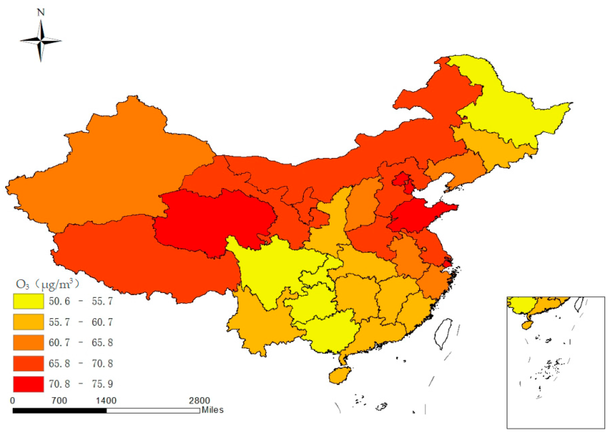
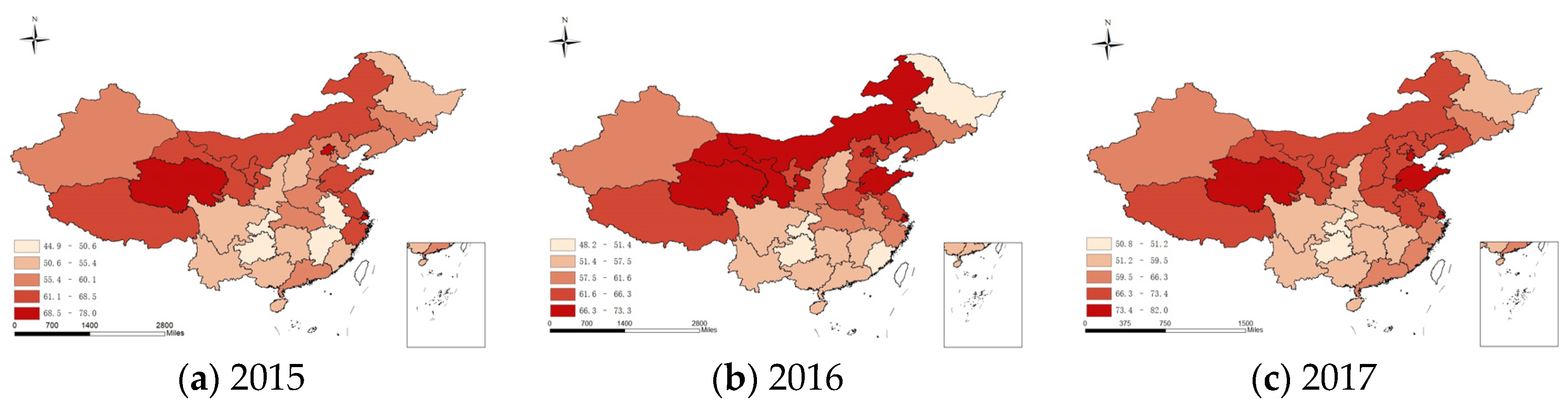
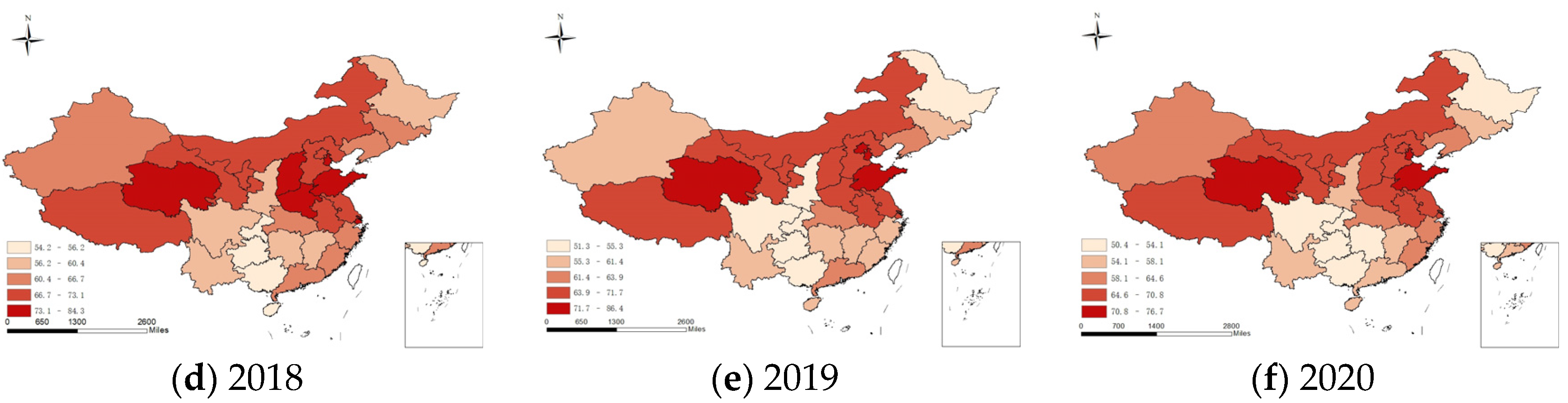
In order to examine the spatial alterations in the yearly average O3 concentration across 338 cities in mainland China between 2015 and 2020, this study evaluated the annual average O3 concentration in all Chinese cities utilizing ArcGIS software. Figure 1 illustrates the spatial distribution of the six-year average O3 concentration. Over this period, Tianjin emerged as the most polluted city, exhibiting an annual average O3 concentration of 75.9 µg/m3. Conversely, Chongqing displayed the lowest O3 pollution at 75.9 µg/m3, while Hainan reported a median O3 concentration of 56.3 µg/m3. An analysis of the spatial variation characteristics, as depicted in Figure 1, reveals significant spatial heterogeneity in the national O3 concentration. In the six years spanning 2015–2020, the most polluted areas were Beijing and Tianjin in North China, Shandong and Shanghai in East China, and Qinghai in Northwest China. The average annual O3 concentrations in these regions were 66.5, 71.6, 70.6, 72.9, 68.5, and 67.7 µg/m3, respectively. Some areas in Tibet, Gansu, and Ningxia in Northwest China, Inner Mongolia in North China, Henan in Central China, and Jiangsu in the Yangtze River Delta also experienced significant pollution. Following economic development in the eastern region, particularly in the Yangtze River Delta, population growth and industrial activities surged, leading to the release of large quantities of atmospheric pollutants including NOx and VOCs. These pollutants provided sufficient precursors for O3 generation, exacerbating O3 pollution [31]. However, certain cities in northwest China are characterized by low terrain, which does not facilitate the diffusion of air pollutants, allowing pollutants to accumulate easily, including in the central region of Gansu Province [44]. Consequently, these regions exhibited elevated average annual O3 concentrations. Areas like Chongqing, Sichuan, Guizhou, and Guangxi in the west and Heilongjiang in the northeast displayed lower pollution levels. The temporal and spatial distribution of VOC characteristics and sources may significantly differ across China due to variations in industrial structure, geography, meteorology, and seasonal and diurnal shifts between regions [45]. For instance, Chongqing possesses unique topographic conditions and superior air circulation compared to the Chengdu plains, resulting in enhanced pollutant diffusion in this area [46]. Regarding interannual spatial changes, the spatial distribution of O3 concentration in 2016 closely resembled that in 2015 (Figure 2a,b), demonstrating a spatial pattern with higher O3 concentrations in the north and lower concentrations in the south, predominantly in the Yangtze River Delta and some northwest regions. In 2017, high O3 concentrations extended southward across the North China Plain (Figure 2c), while low concentrations declined. In 2018, high O3 concentration areas were mainly located in the North China Plain and some parts of Northwest China (Figure 2d), mainly in Qinghai, Shandong, Henan, and Shanxi. The spatial distribution of O3 levels in 2019 and 2020 was akin to that observed in 2017 and 2018 (Figure 2e,f); however, the high O3 concentration zone in the northern region diminished. Tianjin recorded the highest O3 concentration in 2020, a significant increase from its 11th-place ranking in 2015, while Shanghai, which had the third-highest O3 concentration in 2015, experienced a notable decline in its ranking in 2020. Tianjin, an established industrial base in China, has experienced a significant increase in industrial activities and automobile usage in recent years, leading to elevated emissions of VOCs and NOx. Consequently, there has been a substantial rise in anthropogenic precursor O3 emissions [47]. In contrast, the O3 issue in Shanghai is linked to its sizable population and economic scale. Recently, the implementation of stringent policies to curb local emissions has diminished the prevalence of high O3 concentrations, thereby alleviating the ozone problem in Shanghai [48].
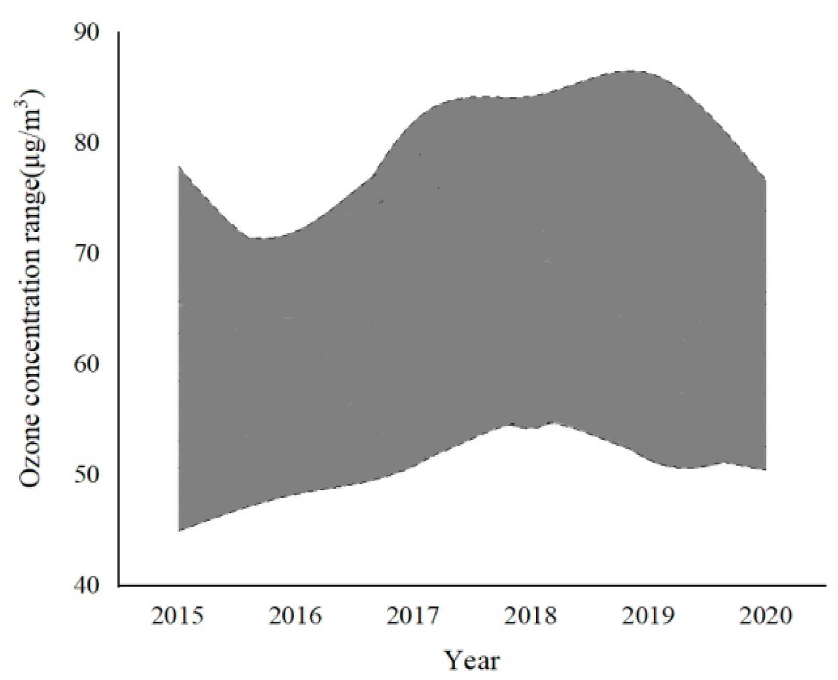
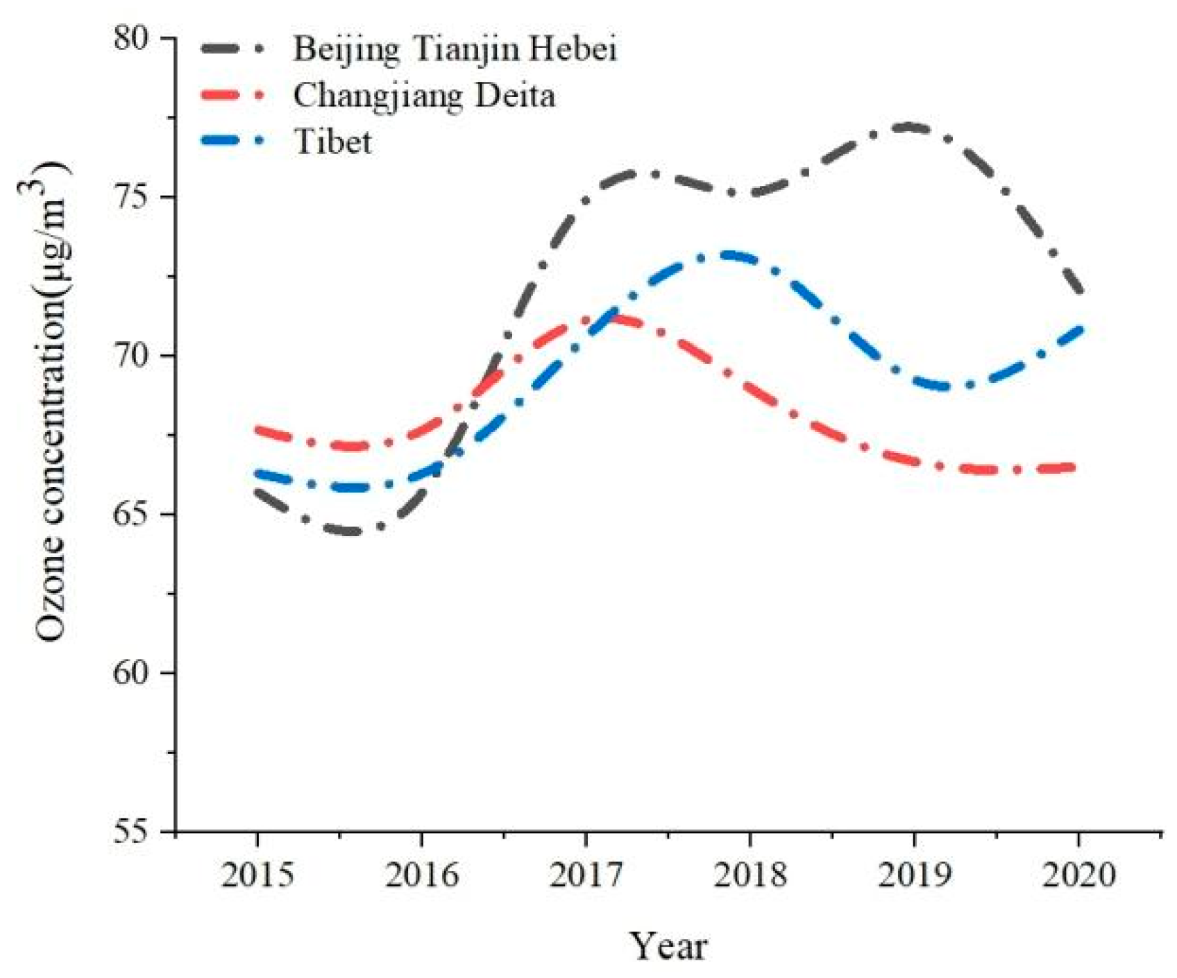
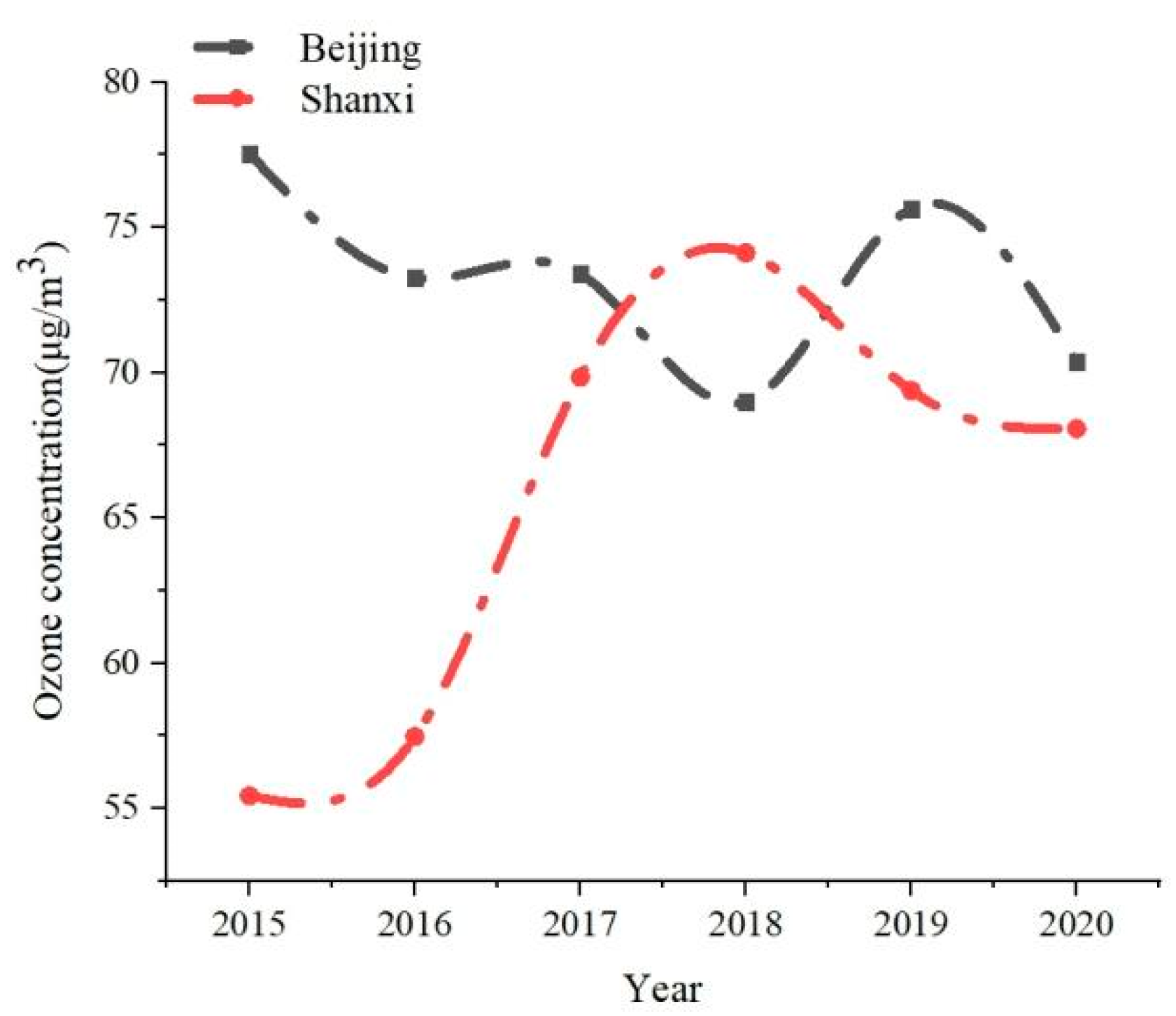
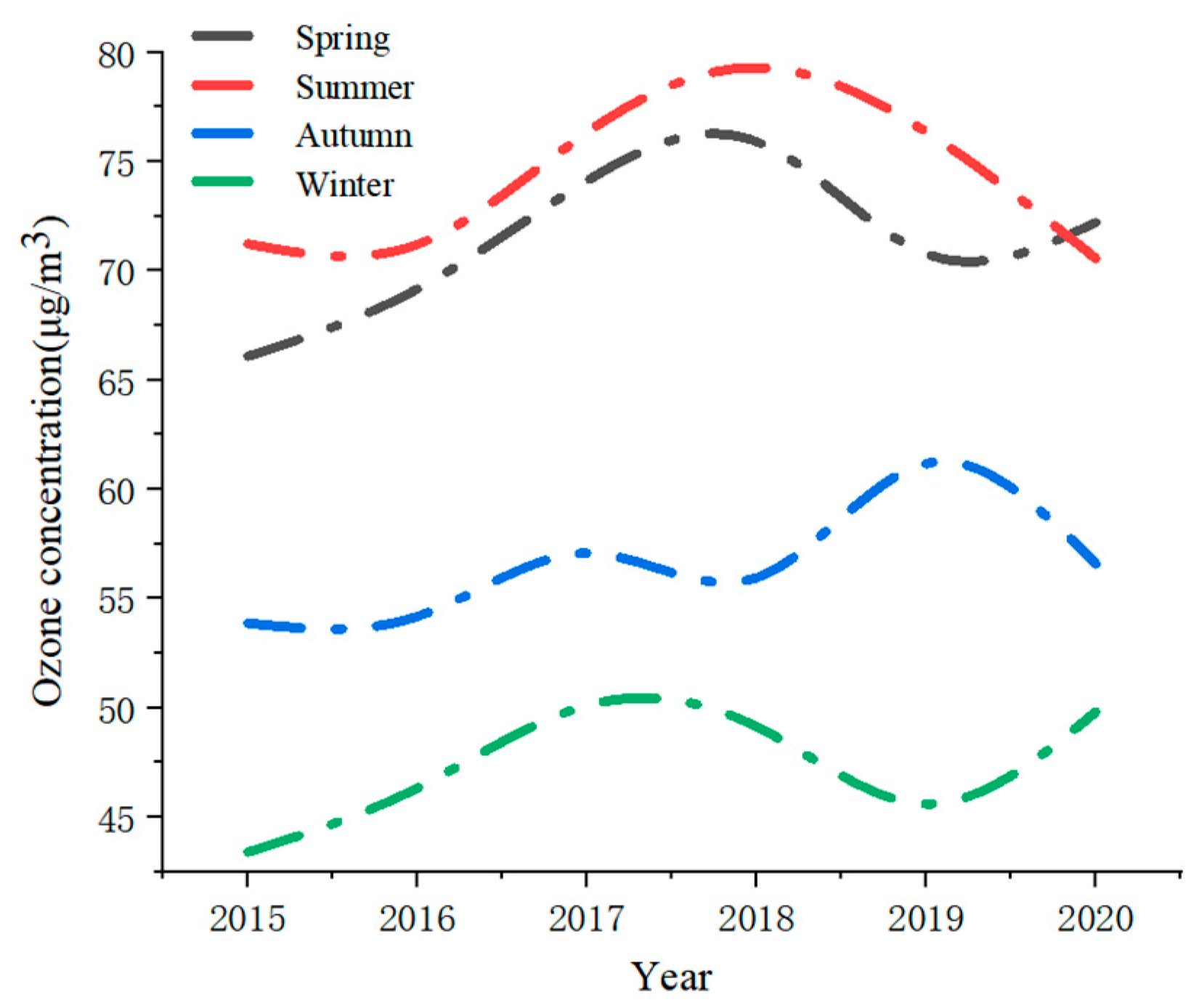
The average annual ozone concentrations in all Chinese cities from 2015 to 2020 were 58.7, 60.2, 64.4, 65.1, 63.5, and 62.3 µg/m3, respectively. The O3 concentration range for each province gradually increased from 38.6–74.8 µg/m3 in 2015 to 42.6–82.1 µg/m3 in 2019. In total, the O3 concentration experienced a slow growth of 9.1% over five years, with an average annual increase of 0.66 µg/m3 and a slight decline after 2019 (Figure 3). This occurred as a result of urbanization which increased anthropogenic industrial emissions and high NOx emissions, providing sufficient precursors for O3 generation and causing severe atmospheric O3 pollution [49]. However, in 2020, the Chinese government enforced strict control measures, and the COVID-19 pandemic contributed to the reduction in O3 concentration [39]. From a regional perspective (Figure 4), areas with high O3 concentrations between 2015 and 2020 included the Beijing-Tianjin-Hebei region, the Yangtze River Delta (Shanghai, Jiangsu, Zhejiang), and Tibet, with O3 concentrations of 65.7–77.2 µg/m3, 66.2–71.1 µg/m3, and 62.9–73.0 µg/m3, separately. This indicates that most of these provinces have developed industries and significant O3 pollution. In most regions, O3 concentrations decreased after 2019, primarily due to a reduction in VOC emissions and improvements in meteorological conditions related to pollution [50]. Since Tibet encompasses a vast area with diverse climates, surface O3 concentrations in the region exhibit significant variations [51]. The provinces with the largest changes in O3 concentrations between 2015 and 2020 were Beijing and Shanxi (Figure 5). The O3 concentration in Beijing decreased from 77.5 µg/m3 in 2015 to 70.4 µg/m3 in 2020, likely due to the city’s numerous air pollution reduction initiatives, including phasing out obsolete vehicles and replacing coal with clean energy sources [52]. The reduction in automobile emissions and improvement of fuel standards led to a decreased influence of NOx on O3. Conversely, the O3 concentration in Shanxi Province increased from 55.4 µg/m3 in 2015 to 68.1 µg/m3 in 2020. As a crucial national energy base and China’s largest coal-producing province, Shanxi’s residential and commercial areas are concentrated in valleys and basins. The unique geography and unfavorable meteorological conditions, such as local circulation and temperature inversion, hinder the dispersion of pollutants [53], resulting in a gradual increase in O3 concentration. Regarding seasonal variation (Figure 6), O3 pollution in spring and summer between 2015 and 2020 was notably severe, with an extensive spatial range. The mean concentration of O3 in summer was 74.2 µg/m3, while in spring, autumn, and winter, it was 71.4, 56.5, and 47.4 µg/m3, respectively. The regions with high O3 concentrations switched between spring and summer. Additionally, the concentration of O3 was higher in autumn than in winter. The higher concentration of O3 in the air during spring and summer is due to the occurrence of photochemical reactions, which are more favorable for O3 formation under high temperatures and intense solar radiation. Such conditions exacerbate O3 pollution [54]. Conversely, in autumn and winter, the increase in pollution emissions, amplified temperature inversion, and relatively stable atmospheric stratification do not facilitate the local transport of pollutants or their dilution and dispersion [35].
3.2. Spatial Aggregation Characteristics of O3
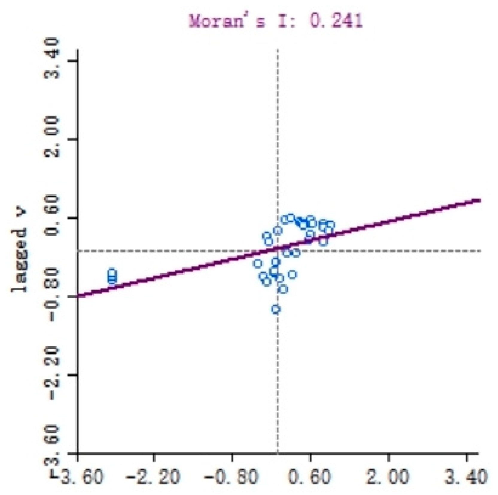
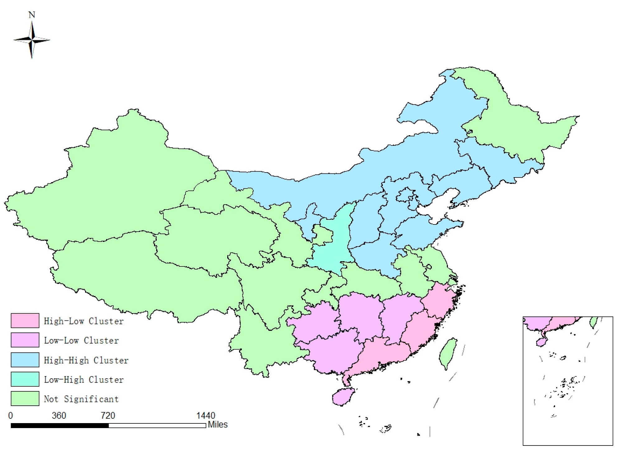
To investigate whether there was spatial autocorrelation of O3 concentration among provinces in China, a spatial autocorrelation analysis was performed on O3 concentration in 31 provinces in China from 2015 to 2020. As displayed in Figure 7, the mean annual Moran’s I for O3 concentration passed the 95% significance test and was positive, suggesting that the spatial distribution of O3 concentration in all Chinese provinces had a significant spatial correlation. The Lisa index was utilized to identify five spatial autocorrelation clustering relationship types (Figure 8): (1) “high–high” clustering (HH); (2) low–low clustering (LL); (3) high–low clustering (HL); (4) “low–high” clustering (LH); and (5) no significant agglomeration characteristics. According to the results, the national O3 concentration displayed “high–high” clustering, “low–low” clustering, “low–high” clustering, and “high–low” clustering characteristics. The “high–high” clustering types were primarily located in the Beijing–Tianjin–Hebei region, Inner Mongolia, Jilin, Liaoning, Shanxi, Shandong, Henan, and Ningxia. The O3 concentration change rate in these regions was relatively high, and they were in the diffusion effect region of O3 concentration growth, leading to an increase in the number of cities with high O3 concentrations that were adjacent to highly polluted areas [55]. In contrast, the clustering area of the change rate of low O3 concentration was primarily distributed in Guizhou, Hunan, Jiangxi, Guangxi, Hainan, and other regions. The urban air diffusion conditions in these regions were favorable and beneficial for the diffusion of pollutants [56], causing a low-low concentration. These cities were surrounded by cities with low O3 concentrations, causing the oxygen concentration to decrease. The high–low cluster type was distributed in Zhejiang, Fujian, and Guangdong. These cities were surrounded by cities with low O3 concentrations and showed spatial agglomeration and cross-regional migration [57]. As a result, the concentration of O3 in cities with high O3 concentration continued to rise, while that of cities with low O3 concentration continued to decline. Shaanxi Province had a low-high clustering distribution, and the high concentration of O3 in neighboring provinces adversely affected Shaanxi.
3.3. Factors Affecting O3 Concentration
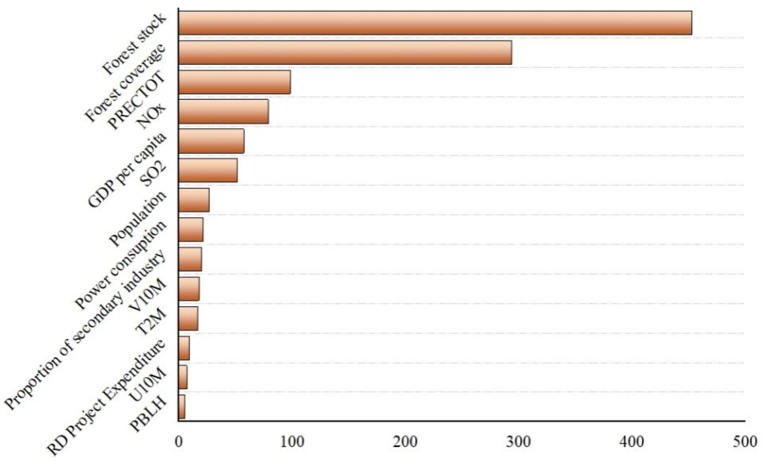
To investigate the spatial autocorrelation of O3, we performed a correlation analysis of 14 meteorological, natural, and socioeconomic factors in each province in China from 2015 to 2020. Considering the spatial correlation, Ordinary Least Squared Regression (OLS) was adopted for estimating the constraint model, and the results indicated that LM-Error (0.034) was statistically more significant than LM-Lag (0.107), leading to the choice of the spatial error model for analysis. In the estimation of OLS, R2 = 0.985, and in the estimation of the spatial error model, R2 = 0.990, showing that accounting for spatial correlation enhances model fit. The findings of the SEM model analysis are presented in Table 1, where a total of 9 variables, including temperature, wind speed, wind direction, per capita GDP, RD project funds, forest stock, forest coverage, SO2, and power consumption, were discovered to make a significant impact on the national O3 concentration. However, the SEM model only presented the linear correlation between variables, whereas some variables might show a nonlinear relationship with O3 concentration. Therefore, a nonlinear model, random forest, was used to improve the accuracy of the simulation of the influencing factors. The random forest result (Figure 9) showed that R2 was 0.503, and along with the above variables, the coefficients of precipitation (98.17) and NOx (78.96) were large, indicating that these factors were significantly correlated with O3 concentration. A multicollinearity test conducted using SPSS26.0 (Table 1) showed that the variance inflation factor (VIF) of wind speed (13.989), NOx (21.233), and power consumption (13.692) was greater than 10, indicating significant collinearity among these three factors.
The regression results demonstrated a significant correlation between precipitation, temperature, wind direction, per capita GDP, RD project funds, forest stock, forest coverage, SO2, and O3 concentration which could be utilized for evaluating the correlation between meteorological, natural, socioeconomic factors, and O3 pollution. The formation, transformation, transport, and removal of O3 are all significantly influenced by meteorological conditions, and all these factors can affect the concentration of O3 [58]. Although precipitation was not significant in the SEM model, its coefficient in the random forest model was larger (98.17), indicating that precipitation significantly influenced O3 concentration. This may be due to the scouring effect of precipitation on air pollutants. Particles converge and settle on the ground through sedimentation, reducing atmospheric O3 concentration. Therefore, precipitation promotes the reduction of O3 concentration [59]. The temperature and O3 concentration were found to be positively correlated, with a partial regression coefficient of 0.248. The generation of O3 mainly depends on high temperatures and intense solar radiation [60]. The urban heat island effect and air pollution resulting from increased anthropogenic emissions are major environmental problems in urban areas [61]. Urbanization increases heat emission from natural heating systems and man-made sources in urban areas, such as indoor heating and air conditioning generated by transportation and cooking, which can lead to the urban heat island effect [62]. The heat island effect affects O3 pollution by changing the local cycle and the chemical reaction environment, such as temperature [63]. The findings of the SEM study demonstrated that the effect of wind direction on O3 concentration was negative (−2.702). O3 transport is mainly driven by the wind. When the wind gets stronger, the boundary layer becomes higher, which favors the diffusion of O3. The direction of the wind not only affects the direction of diffusion of O3 [64] but also leads to the contaminants for land-based air to build up.
During autumn and winter, the local transport, dilution, and diffusion of pollutants are not favored due to an increase in pollutant emissions, frequent temperature inversion, and relatively stable atmospheric stratification [35]. We observed a negative correlation between SO2 and O3 (−0.14). As the concentration of SO2 decreases significantly, the pollution of O3 increases, probably due to the complex physical and chemical mechanisms within the region where O3 interacts with specific pollutants, such as SO2 [65]. An increase in the concentration of SO2 enhances sulfate production, increases aerosol concentrations, weakens atmospheric photochemical reactions, and thus increases the uptake of HO2 radicals. However, nitrogen oxides in the air can undergo photochemical reactions under ultraviolet light and dissociate to form various free radicals, which can further react with oxygen molecules (O2) in the atmosphere to produce O3 [66] under the catalysis of ultraviolet light. Therefore, an increase in the SO2 concentration decreases the O3 concentration.
In the SLM, per capita GDP was positively correlated with O3 concentration (0.00007). Per-capita GDP reflects the socioeconomic growth of a region and indicates socioeconomic development, regional planning, and environmental protection, and thus, it can affect changes in O3 [58]. Over the past six years, China’s per capita GDP increased from 49,500 yuan in 2015 to 70,700 yuan in 2020, growing at an average annual rate of 35.3% over the preceding six years. The growth rate was relatively high, and energy consumption was high, with coal serving as the main energy source in recent decades, leading to high O3 emissions [67]. However, some studies have found an inverted U-shaped distribution between China’s GDP and O3 concentration, mainly due to wide regional disparities. Additionally, the effect of GDP on O3 varied greatly among regions at different developmental stages [68]. The correlation between economic development and ecological health in economically developed areas crossed the EKC inflection point, and per capita GDP was negatively related to O3 concentration, while in economically underdeveloped areas, the mode of economic development has changed from extensive to centralized, promoting environmental improvement [23]. For example, in Ningxia, O3 increased from 62.8 µg/m3 in 2015 to 65.5 µg/m3 in 2020, with an increase rate of 4.3%, and per capita GDP increased from 378.76 million yuan in 2015 to 550.21 million yuan in 2020, with an increase rate of 45.3%.
The SEM results showed a negative correlation (−0.0000012) between the expenditure on RD projects and O3 concentration. Expenditure on science and technology had a decreasing impact on O3 concentration. A 1% increase in technological innovation difference can increase the degree of O3 pollution control cooperation by 8.7%. High-tech industries play a strategic role in China [64]. Investments in R&D and resulting technological progress promote energy efficiency and pollution treatment technology, leading to a decrease in pollutant emissions and improvement in the pollution treatment rate, thereby promoting the inter-regional collaborative treatment of air pollution [1]. Increasing investment in environmental governance and using new technology can enhance the atmospheric environment for sustainable economic development, particularly in Northeast and North China, which are dominated by the secondary industry [69]. The phased rule of technological progress indicates that regions with higher technological levels have a greater investment in pollution control, higher resource utilization efficiency, a larger scale of regional production activities, higher demand for resources and energy, and lower O3 emission per unit output [68]. Thus, technological progress significantly affects air quality improvement. Additionally, cities with stronger economic growth make greater investments in reducing pollution [59].
3.4. The Impact of Regional Factors on O3 Concentration
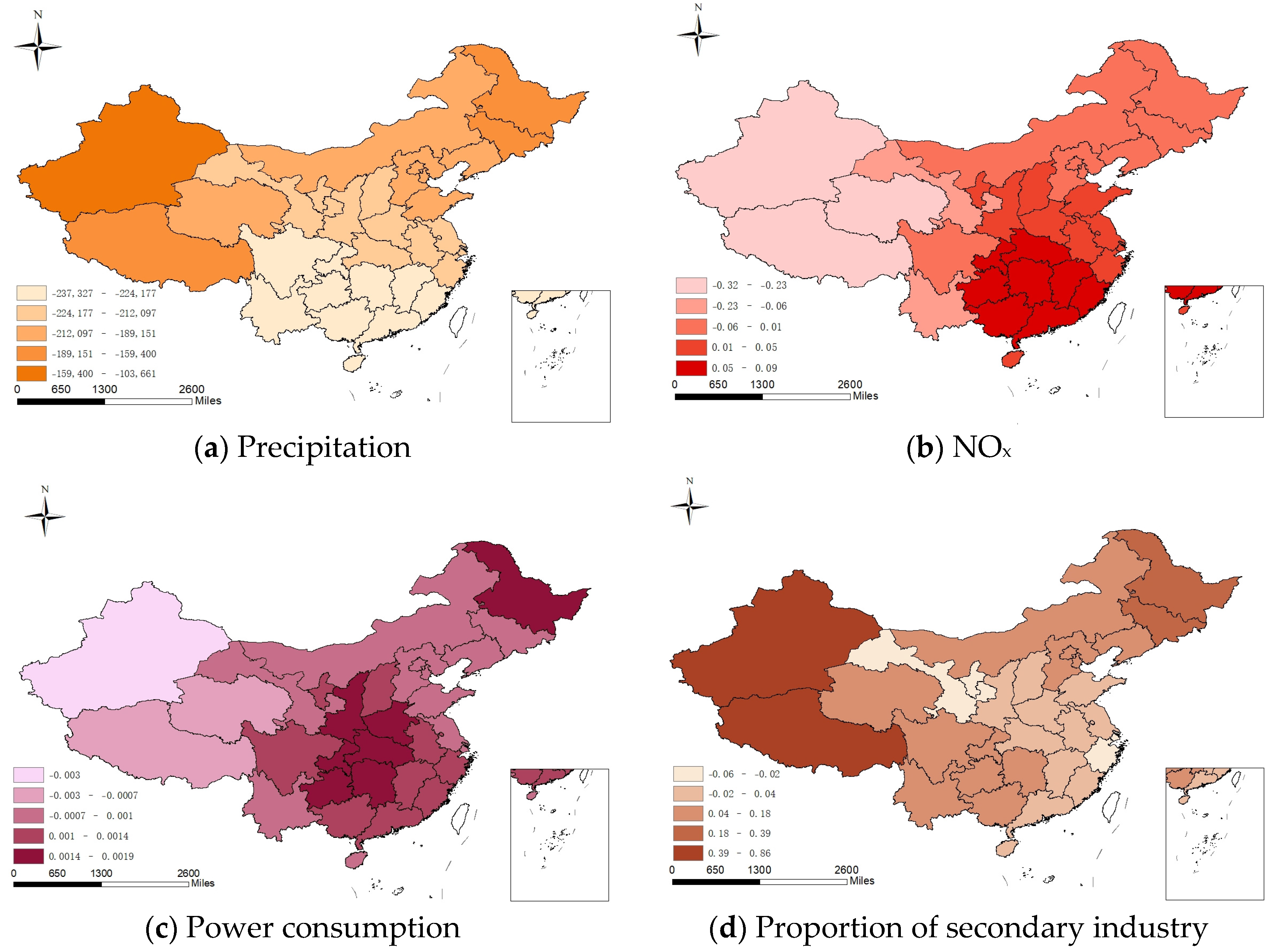
Although the SEM model demonstrated that multiple variables influenced O3 concentration across China, it only revealed the global correlation between these variables and O3 without considering regional implications. Consequently, we utilized the GWR model to further investigate the correlation between O3 concentration and regional meteorological, natural, and socioeconomic factors. We examined the correlation of 14 variables, eliminating those with significantly high Pearson’s correlation. Using the GWR model, we measured R2 values greater than 0.5 and identified 10 unrelated variables, including precipitation, wind speed, wind direction, NOx, population, per capita GDP, forest stock, RD project funds, electricity consumption, and the proportion of secondary industry (Table 2). In this study, we used the variables precipitation, NOx, electricity consumption, and the proportion of secondary industry for analysis.
The impact of precipitation on O3 formation in cities with different geographical locations was negative (Figure 10a). The maximum O3 concentration occurred when precipitation was lowest [70]. Guangdong, an old industrial base with high industrial development, experienced more precipitation. Air convection and heavy precipitation facilitated the removal and clearing of accumulated O3 in this region [71]. Jiangsu and Zhejiang, situated in the middle latitudes of the eastern coast of the mainland, belong to the subtropical monsoon climate with a unique weather condition called Meiyu [72]. This region had high atmospheric water vapor content, extensive cloud cover, and abundant annual precipitation. The purification effect of precipitation on O3 exceeded its generation rate, promoting O3 reduction. As rainfall duration increased, the removal effect of O3 in Sichuan Province also increased. This phenomenon was likely due to cloud cover, which reduced solar radiation and photochemical reactions. In terms of precipitation, a longer duration of rainfall implied a more significant negative impact on O3 generation [73]. Precipitation also affected O3 production by removing precursors. In regions like Hainan and Guangxi, the upward transport and diffusion of water vapor were greater [74], leading to increased cloud cover and urban precipitation, ultimately decreasing O3 concentration.
There are two primary sources of nitrogen oxide emissions in the troposphere: anthropogenic (e.g., thermal power plants, transportation, industrial, and residential use) and natural (lightning, biomass burning, and soil) [75]. In different areas, the influence of NOx on surface O3 varied, sometimes even being opposite (Figure 10b). In the NOx control area, NOx drove O3 concentration, suggesting that reducing NOx could significantly lower O3 concentration. In southeast China, after removing meteorological factors, O3 concentration decreased, indicating a NOx-limiting or mixed-sensitive O3 formation mechanism in the area [76]. The O3 concentration was most significantly impacted by NOx emissions in the Pearl River Delta region and central and western regions like Jiangxi, Anhui, Guangxi, Guizhou, and Qinghai (Figure 10b). Because of rapid urbanization and industrialization in western China, anthropogenic emission changes were the primary driving factors of NO2 alterations in most western provinces, with growth linked to the region’s fast industrialization and urbanization after the “Great Western Development” movement [77]. The concentrations of NO2 and O3 in Guangzhou showed opposing patterns, indicating that VOCs limited O3 generation. After 2017, with the removal of meteorological factors, NO2 and O3 concentrations in Guangzhou significantly decreased, signifying a change in the O3 formation mechanism from VOC-limiting to mixed-sensitivity or NOx-limiting due to a sharp decline in NOx emissions [76]. The Pearl River Delta boasts a high degree of urbanization in China, with mobile and industrial sources being the primary contributors to NOx emissions in this area. The rapid increase in automobile ownership and the effective management of pollutants from large power plants have been the main drivers of NOx concentration growth [78]. In contrast, most urban clusters intermixed with industrial bases in northeastern China (north of 30° N) were VOC-limiting areas [79], with NOx mitigating O3 formation and decreasing O3 concentration in northeastern regions such as Heilongjiang, Jilin, and Liaoning [80]. The opposing trends in Guangzhou’s NO2 and O3 concentrations before 2017 suggested that VOCs limited O3 generation. After 2017, upon removing meteorological factors, NO2 and O3 concentrations in Guangzhou significantly declined, indicating that the O3 formation mechanism shifted from VOC-limiting to mixed-sensitivity or NOx-limiting due to the dramatic decrease in NOx emissions [76]. The Pearl River Delta is highly urbanized within China, and mobile and industrial sources are the main contributors to NOx emissions in the region. The rapidly increasing number of automobiles and the effective control of pollutants from large power plants have been the primary causes of the increase in NOx concentration [78].
Power consumption and O3 concentration exhibited a negative correlation in Xinjiang, Qinghai, and Tibet, while they were significantly positively correlated in Guangdong, Heilongjiang, Jiangxi, Hubei, Guangxi, and Guizhou (Figure 10c). Central regions such as Jiangxi and Hubei [81,82] have abundant industrial sources and numerous thermal power plants. Industrial and total power consumptions were relatively high, leading to the emission of large O3 concentrations. Moreover, NOx and VOCs in waste gas generated during the thermal power production process can stimulate O3 formation. The positive effect of electricity consumption on O3 concentration in the Pearl River Delta region may be related to energy use and policy adjustment. The implementation of the “coal to electricity” policy and the promotion of new energy vehicles in recent years have led to a year-by-year increase in electricity consumption, subsequently increasing O3 pollution [83]. Some parts of Northeast China, such as Heilongjiang, differ from other Chinese megacities due to their extremely cold winters (daily average temperatures below −20 °C) and complex emission sources like central heating systems and coal-fired power plants, which contribute to the emission of more industrial pollutants [28,84]. Western regions like Guizhou and Guangxi are important energy producers (due to the “west-east power transmission” initiative) and heavy industrial bases (focused on mining, fossil fuels, and raw materials). In contrast, residential power supply and heating emissions in Qinghai [85] and other areas were found to be lower, while exhaust gas from energy-intensive industries was primarily responsible for high O3 concentration emissions.
Although the proportion of secondary industry in the Beijing-Tianjin-Hebei region, Liaoning, Jilin, Heilongjiang, and western regions such as Xinjiang, Tibet, Sichuan, Yunnan, and Guizhou showed a significant positive correlation with O3 concentration (Figure 10d), the differences in industrial development stages across these regions were substantial. The eastern region had a well-developed light industry, and the high-tech industry was more advanced than in the central and western regions. The average annual R&D investment in the Beijing–Tianjin–Hebei region amounted to 5.88 billion yuan from 1999 to 2015, compared to only 83 million and 66 million yuan in central and western regions, respectively, in accordance with the Statistical Yearbook of China’s High-tech Industry [86]. Northeast China is a crucial hub for both agricultural and industrial production within China. The region’s industrial structure is primarily focused on heavy chemical manufacturing and benefits from robust industrial infrastructure. Pollution in the region is predominantly attributed to the steel, machinery, petroleum, and chemical industries, with coal combustion, automobile exhaust, and petrochemical emissions being the primary sources of pollutants [87]. The western region of Northeast China is characterized by high energy consumption and an abundance of coal and mineral resources, resulting in the presence of high-pollution industries such as smelting, oil mining, and mineral extraction.
4. Conclusions and Policy Implications
The present study examined the spatiotemporal variation characteristics of O3 concentration across China using spatial econometric models, stochastic forest models, and GWR analysis. The study investigates the correlation between meteorological, natural, and socioeconomic factors with O3 concentration. Our results show significant spatial heterogeneity and agglomeration of O3 concentration across the country, with Beijing, Tianjin, Shandong, and Qinghai being the most polluted regions. Conversely, Chongqing, Guizhou, Guangxi, and Heilongjiang have lower levels of O3 pollution. From 2015 to 2019, the annual O3 concentration tended to increase initially but slightly decreased thereafter. The study identified eight significant factors in determining the spatial distribution of O3 concentration, with meteorological, natural, and socioeconomic factors playing crucial roles. Precipitation, temperature, and per capita GDP positively influence O3 concentration, while wind direction, RD project cost, forest stock, forest coverage, and SO2 have negative effects. The study indicates that meteorological, natural, and socioeconomic factors have a strong spatial dependence on O3 concentration, and recent severe O3 pollution in the Pearl River Delta and central and western regions of China including Jiangxi, Guangxi, and Guizhou. These results indicated that residential energy use and industrial source emissions strongly affected air pollution in the Pearl River Delta and the central and western regions. Additionally, the proportion of the secondary industry significantly affected pollution in Northeast China, demonstrating that the secondary industry immensely contributed to economic growth. Although industrial coal burning is a significant contributor to high O3 pollution, high-tech industries are becoming increasingly responsible for O3 pollution in the Beijing–Tianjin–Hebei region. By contrast, the influence of meteorological, natural, and socioeconomic factors on O3 pollution in eastern China is relatively stable. High-energy-use and high-pollution industries contribute to O3 pollution in Xinjiang, Tibet, and other western regions, highlighting the need for better energy conservation and emissions reduction strategies.
Based on these findings, we propose the following policy recommendations:
- (1)
- Recently, the concentration of O3 in Chinese cities has increased, especially in highly developed areas like the Beijing–Tianjin–Hebei region and the Yangtze River Delta, where O3 pollution is even more serious. Besides this, some industrial cities in western China have serious O3 pollution problems. Most studies were performed only in heavily polluted areas; however, the mechanism of O3 source, favorable weather conditions, and exogenous transport characteristics in areas with lower levels of pollution have not been systematically explored. To control air pollution more effectively, different development stages of provinces and their environmental capacities. Therefore, a regional division of O3 pollution control should be established, and strategies for reducing key pollutants in different regions should be developed to form a collaborative atmospheric environment management system that fosters fine governance;
- (2)
- To control O3 emissions in areas including the Pearl River Delta and the central and western regions of Jiangxi, Anhui, Guangxi, Guizhou, and Qinghai, reducing NOx emissions from industrial sources and motor vehicle exhaust is essential. Strategies such as replacing coal with clean energy, upgrading old cars with new ones, phasing out old cars with subsidies, and developing public transport could effectively reduce NOx emissions. Additionally, regulating meteorological variations, such as creating artificial rain during summer, could help reduce O3 concentrations;
- (3)
- As for the industrial enterprises with high energy consumption and high pollution, efforts should be made to develop high-quality and efficient clean energy (including nuclear power and wind power), high-tech industries, and modern service industries to satisfy the requirements of optimizing the industrial and energy consumption structure. At the same time, air pollution is the result of industrial production, urban construction, residents’ lifestyles, and other factors. Therefore, local governments should establish a multidisciplinary cooperative control mechanism in order to create a healthy balance [88].
Our study has certain limitations. Firstly, the variables collected were not comprehensive, and some variables had missing data. However, it is essential to consider other factors that could potentially impact O3 concentration. If additional data become available in the future, the indicators of all factors could be significantly improved, enabling a more comprehensive and systematic study. Secondly, the sample size of the study was not large enough, and more extended periods of observations and continuous research are required to obtain more accurate results.
Author Contributions
H.L. and Y.Z. conceived and designed the study. H.L. and Y.Z. processed the data and performed analysis. H.L. and Y.Z. contributed to the interpretation of the results. H.L. and Y.Z. wrote the paper. All authors reviewed and edited the draft, approved the submitted manuscript, and agreed to be listed and accepted the version for publication. All authors have read and agreed to the published version of the manuscript.
Funding
The current work was supported by Beijing Natural Science Foundation (No.: 9212015).
Institutional Review Board Statement
Not applicable.
Informed Consent Statement
Not applicable.
Data Availability Statement
Not applicable.
Conflicts of Interest
The authors declare no conflict of interest.
References
- Guo, Y.M.; Lin, X.Q.; Bian, Y. Spatio-temporal evolution of air quality in urban agglomerations in China and its influencing factors. Ecol. Econ. 2019, 35, 167–175. [Google Scholar]
- Liu, B.J. Strengthening the collaborative control of PM2.5 and ozone and deepening the battle of blue sky protection. Environ. Monit. China 2021, 69, 40–43. [Google Scholar] [CrossRef] [PubMed]
- Avnery, S.; Mauzerall, D.L.; Liu, J.; Horowitz, L.W. Global crop yield reductions due to surface ozone exposure: 1. Year 2000 crop production losses and economic damage. Atmos. Environ. 2011, 45, 2284–2296. [Google Scholar] [CrossRef]
- Rios, B.; Estrada, F. Reduction in crop yield in Mexico due to ozone associated with emissions from biomass burning. Water Air Soil Pollut. 2022, 233, 407. [Google Scholar] [CrossRef]
- Zhang, J.F.; Wei, Y.J.; Fang, Z.F. Ozone pollution: A major health hazard worldwide. Front. Immunol. 2019, 10, 2518. [Google Scholar] [CrossRef] [Green Version]
- Feng, Z.; De Marco, A.; Anav, A.; Gualtieri, M.; Sicard, P.; Tian, H.; Fornasier, F.; Tao, F.; Guo, A.; Paoletti, E. Economic losses due to ozone impacts on human health, forest productivity and crop yield across China. Environ. Int. 2019, 131, 104966. [Google Scholar] [CrossRef]
- Stowell, J.D.; Kim, Y.-M.; Gao, Y.; Fu, J.S.; Chang, H.H.; Liu, Y. The impact of climate change and emissions control on future ozone levels: Implications for human health. Environ. Int. 2017, 108, 41–50. [Google Scholar] [CrossRef]
- Nuvolone, D.; Petri, D.; Voller, F. The effects of ozone on human health. Environ. Sci. Pollut. Res. 2018, 25, 8074–8088. [Google Scholar] [CrossRef]
- Dong, Z.X.; Ding, D.; Jiang, Y.Q.; Zheng, H.T.; Xing, J.; Wang, S.X. Response of PM2.5 and ozone to emission reduction of precursors and climate change and its policy implications. Res. Environ. Sci. 2022, 36, 223–236. [Google Scholar] [CrossRef]
- Song, J.; Li, C.; Liu, M.; Hu, Y.; Wu, W. Spatiotemporal distribution patterns and exposure risks of PM2.5 pollution in China. Remote Sens. 2022, 14, 3173. [Google Scholar] [CrossRef]
- Wang, X.Z.; Zhao, S.; Guo, L.H.; Zhang, H.B.; Gao, J.B. Seasonal variation of ozone in “2+26” cities in Beijing-Tianjin-Hebei region and its surrounding areas. Res. Environ. Sci. 2022, 35, 1786–1797. [Google Scholar] [CrossRef]
- He, C.; Yang, L.; Cai, B.; Ruan, Q.; Hong, S.; Wang, Z. Impacts of the COVID-19 event on the NOx emissions of key polluting enterprises in China. Appl. Energy 2021, 281, 116042. [Google Scholar] [CrossRef] [PubMed]
- Ma, Q.; Wang, W.; Wu, Y.; Wang, F.; Jin, L.; Song, X.; Han, Y.; Zhang, R.; Zhang, D. Haze caused by NOx oxidation under restricted residential and industrial activities in a mega city in the south of North China Plain. Chemosphere 2022, 305, 135489. [Google Scholar] [CrossRef] [PubMed]
- Jin, J.Q.; Du, Y.; Xu, L.J.; Chen, Z.Y.; Chen, J.J.; Wu, Y.; Ou, C.Q. Using Bayesian spatio-temporal model to determine the socio-economic and meteorological factors influencing ambient PM2.5 levels in 109 Chinese cities. Environ. Pollut. 2019, 254, 113023. [Google Scholar] [CrossRef]
- Yang, Y.; Lan, H.F.; Li, J. Spatial econometric analysis of the impact of socioeconomic factors on PM2.5 concentration in China’s inland cities: A case study from chengdu plain economic zone. Int. J. Environ. Res. Public Health 2020, 17, 74. [Google Scholar] [CrossRef] [Green Version]
- Yan, D.; Ren, X.H.; Kong, Y.; Ye, B.; Liao, Z.Y. The heterogeneous effects of socioeconomic determinants on PM2.5 concentrations using a two-step panel quantile regression. Appl. Energy 2020, 272, 115246. [Google Scholar] [CrossRef]
- Geng, J.C.; Shen, S.; Cheng, C.X. Spatial and temporal distribution of PM2.5 in the Yellow River Basin during the 13th Five-Year Plan period and its multi-scale socioeconomic impact mechanism. J. Geoinform. Sci. 2022, 24, 1163–1175. [Google Scholar] [CrossRef]
- Chen, J.; Zhou, C.; Wang, S.; Li, S. Impacts of energy consumption structure, energy intensity, economic growth, urbanization on PM2.5 concentrations in countries globally. Appl. Energy 2018, 230, 94–105. [Google Scholar] [CrossRef]
- Wang, X.M.; Tian, G.H.; Yang, D.Y.; Zhang, W.X.; Lu, D.B.; Liu, Z.M. Responses of PM2.5 pollution to urbanization in China. Energy Policy 2018, 123, 602–610. [Google Scholar] [CrossRef]
- Qi, G.Z.; Wang, Z.B.; Wei, L.J.; Wang, Z.X. Multidimensional effects of urbanization on PM2.5 concentration in China. Environ. Sci. Pollut. Res. 2022, 29, 77081–77096. [Google Scholar] [CrossRef]
- Jiang, L.; He, S.X.; Cui, Y.Z.; Zhou, H.F.; Kong, H. Effects of the socio-economic influencing factors on SO2 pollution in Chinese cities: A spatial econometric analysis based on satellite observed data. J. Environ. Manag. 2020, 268, 110667. [Google Scholar] [CrossRef] [PubMed]
- Dong, H.; Cheng, L.; Wang, H.Y.; Zhao, X.H.; Zhu, Y. Analysis of ozone pollution characteristics and meteorological influencing factors in Anhui Province. Environ. Monit. China 2021, 37, 58–68. [Google Scholar] [CrossRef]
- Gong, X.S.; Ke, B.Q.; He, C. Spatial-temporal pattern and driving factors of surface ozone in the Yangtze River Economic Belt. Resourc. Environ. Yangtze Basin 2022, 31, 2489–2499. [Google Scholar]
- Liu, X.Y.; Zhao, C.M.; Niu, J.Q.; Su, F.C.; Yao, D.; Xu, F.; Yan, J.H.; Shen, X.Z.; Jin, T. Spatiotemporal patterns and regional transport of ground-level ozone in major urban agglomerations in China. Atmosphere 2022, 13, 301. [Google Scholar] [CrossRef]
- Yang, G.F.; Liu, Y.H.; Li, X.N. Spatiotemporal distribution of ground-level ozone in China at a city level. Sci. Rep. 2020, 10, 7229. [Google Scholar] [CrossRef]
- Cahyadi, M.N.; Handayani, H.H.; Warmadewanthi, I.D.A.A.; Rokhmana, C.A.; Sulistiawan, S.S.; Waloedjo, C.S.; Raharjo, A.B.; Atok, M.; Navisa, S.C.; Wulansari, M.; et al. Spatiotemporal Analysis for COVID-19 Delta Variant Using GIS-Based Air Parameter and Spatial Modeling. J. Int. Environ. Res. Public Health 2022, 19, 1614. [Google Scholar] [CrossRef]
- Qi, J.; Mo, Z.; Yuan, B.; Huang, S.; Huangfu, Y.; Wang, Z.; Li, X.; Yang, S.; Wang, W.; Zhao, Y.; et al. An observation approach in evaluation of ozone production to precursor changes during the COVID-19 lockdown. J. Atmos. Environ. 2021, 262, 118618. [Google Scholar] [CrossRef]
- Yang, G.F.; Liu, Y.H.; Li, W.L.; Zhou, Z.Y. Association analysis between socioeconomic factors and urban ozone pollution in China. Environ. Sci. Pollut. Res. 2023, 30, 17597–17611. [Google Scholar] [CrossRef]
- GB 3095–2012; Ambient Air Quality Standards. Ministry of Ecology and Environment the People’s Republic of China: Beijing, China, 2018.
- HJ 663–2013; Technical Specifications for Assessment of Ambient Air Quality (Trial). Ministry of Ecology and Environment the People’s Republic of China: Beijing, China, 2013.
- Yu, R.X.; Liu, M.X.; Li, L.; Song, J.Y.; Sun, R.D.; Zhang, G.J.; Xu, L.; Mu, R.L. Spatial and temporal variations of atmospheric ozone column concentration over the Yangtze River Delta in recent 15 years and its influencing factors. J. Environ. Sci. 2021, 41, 770–784. [Google Scholar] [CrossRef]
- Wang, X.L.; Zhao, W.J.; Li, L.J.; Yang, X.C.; Jiang, J.F.; Sun, S. Spatial and temporal distribution of ozone in China and its influence on social and economic factors. Earth Environ. 2020, 48, 66–75. [Google Scholar] [CrossRef]
- Bonn, B.; von Schneidemesser, E.; Butler, T.; Churkina, G.; Ehlers, C.; Grote, R.; Klemp, D.; Nothard, R.; Schäfer, K.; von Stülpnagel, A. Impact of vegetative emissions on urban ozone and biogenic secondary organic aerosol: Box model study for Berlin, Germany. J. Clean. Prod. 2018, 176, 827–841. [Google Scholar] [CrossRef]
- Bai, J.H.; Guenther, A.; Turnipseed, A.; Duhl, T.; Greenberg, J. Seasonal and interannual variations in whole-ecosystem BVOC emissions from a subtropical plantation in China. Atmos. Environ. 2017, 161, 176–190. [Google Scholar] [CrossRef]
- Wang, Z.B.; Li, J.X.; Liang, L.W. Spatio-temporal evolution of ozone pollution and its influencing factors in the Beijing-Tianjin-Hebei Urban Agglomeration. Environ. Pollut. 2020, 256, 113419. [Google Scholar] [CrossRef]
- Liu, Q.; Xie, W.J.; Xia, J.B. Using semivariogram and Moran’s I techniques to evaluate spatial distribution of soil micronutrients. Commun. Soil Sci. Plant Anal. 2013, 44, 1182–1192. [Google Scholar] [CrossRef]
- Ma, S.Y.; Zhao, Z.X. Spatial econometric analysis of the impact of fiscal science and technology investment on China’s economic growth: Based on the panel data of 285 prefecture-level cities. Explor. Econ. Probl. 2022, 1–12. Available online: https://kns.cnki.net/kns8/Detail?sfield=fn&QueryID=0&CurRec=1&recid=&FileName=JJWS202207001&DbName=CJFDLAST2022&DbCode=CJFD&yx=&pr=&URLID= (accessed on 18 June 2023).
- Yao, F.G.; Ding, X.L. Effects of land finance on urban land use efficiency: An empirical analysis based on spatial econometric model. Bus. Econ. 2023, 12–14. [Google Scholar] [CrossRef]
- Li, M.J.; Wang, M.C.; Wang, F.Y.; Chen, K.K.; Ding, W. Land use classification in Shenzhen based on multi-feature random forest algorithm. World Geol. 2022, 41, 632–640. [Google Scholar]
- Ji, C.Y.; Lin, J. Methanol futures price prediction and trading strategy based on stochastic forest method. Shanghai Manag. Sci. 2023, 45, 113–118. [Google Scholar]
- Breiman, L. Random forests. Mach. Learn. 2001, 45, 5–32. [Google Scholar] [CrossRef] [Green Version]
- Lia, Y.; Cheng, M.M.; Guo, Z.; Zhang, X.Y.; Cui, X.M.; Chen, S.H. Increase in surface ozone over Beijing-Tianjin-Hebei and the surrounding areas of China inferred from satellite retrievals, 2005–2018. Aerosol Air Qual. Res. 2020, 20, 2170–2184. [Google Scholar] [CrossRef] [Green Version]
- Zhang, Y.; Shi, M.; Chen, J.; Fu, S.; Wang, H. Spatiotemporal variations of NO2 and its driving factors in the coastal ports of China. Sci. Total Environ. 2023, 871, 162041. [Google Scholar] [CrossRef] [PubMed]
- Xue, L.K.; Wang, T.; Gao, J.; Ding, A.J.; Zhou, X.H.; Blake, D.R.; Wang, X.F.; Saunders, S.M.; Fan, S.J.; Zuo, H.C. Ground-level ozone in four Chinese cities: Precursors, regional transport and heterogeneous processes. Atmos. Chem. Phys. 2014, 14, 13175–13188. [Google Scholar] [CrossRef] [Green Version]
- Wang, G.; Zhao, N.; Zhang, H.Y.; Li, G.H.; Xin, G. Spatiotemporal distributions of ambient volatile organic compounds in China: Characteristics and sources. Aerosol Air Qual. Res. 2022, 22, 210379. [Google Scholar] [CrossRef]
- Zhang, T.Y.; Shen, N.C.; Zhao, X.; Wang, X.Y.; Zhao, W.J. Spatial and temporal variation of ozone concentration and population exposure risk assessment in Chengdu-Chongqing urban agglomeration from 2015 to 2019. J. Environ. Sci. 2021, 41, 4188–4199. [Google Scholar] [CrossRef]
- Zhang, T.T.; Lin, W.L.; Ran, L.; Ma, Z.Q.; Yao, Q.; Liu, J.L.; Ming, J. Dual-height distribution of ozone and nitrogen oxides during summer in urban Tianjin: An observational study. Aerosol Air Qual. Res. 2020, 20, 2159–2169. [Google Scholar] [CrossRef] [Green Version]
- Ran, L.; Zhao, C.S.; Xu, W.Y.; Han, M.; Lu, X.Q.; Han, S.Q.; Lin, W.L.; Xu, X.B.; Gao, W.; Yu, Q. Ozone production in summer in the megacities of Tianjin and Shanghai, China: A comparative study. Atmos. Chem. Phys. 2012, 12, 7531–7542. [Google Scholar] [CrossRef] [Green Version]
- Yu, R.L.; Lin, Y.L.; Zou, J.H.; Dan, Y.B.; Cheng, C. Review on atmospheric Ozone pollution in China: Formation, spatiotemporal distribution, precursors and affecting factors. Atmosphere 2021, 12, 1675. [Google Scholar] [CrossRef]
- Lin, W.P.; Guo, X.Z. Spatial and temporal distribution of ozone in urban agglomerations in China. Chin. J. Environ. Sci. 2022, 42, 2481–2494. [Google Scholar] [CrossRef]
- Chen, Y.; Zhou, Y.Q.; Zhang, H.F.; Wang, C.H.; Wang, X.P. Spatiotemporal variations of surface ozone and its influencing factors across Tibet: A Geodetector-based study. Sci. Total Environ. 2022, 813, 152651. [Google Scholar] [CrossRef]
- Tang, G.Q.; Liu, Y.S.; Zhang, J.Q.; Liu, B.X.; Li, Q.H.; Sun, J.; Wang, Y.H.; Xuan, Y.J.; Li, Y.T.; Pan, J.X. Bypassing the NOx titration trap in ozone pollution control in Beijing. Atmos. Res. 2021, 249, 105333. [Google Scholar] [CrossRef]
- Chen, L.; Xiao, H.; Zhu, L.Y.; Guo, X.; Wang, W.Y.; Ma, L.; Guo, W.; He, J.Y.; Wang, Y.; Li, M.M. Characteristics of Ozone pollution and the impacts of related meteorological factors in Shanxi Province, China. Atmosphere 2022, 13, 1729. [Google Scholar] [CrossRef]
- Cui, M.R.; Bai, L.Y.; Feng, J.Z.; Lin, X.S.; Li, H.L.; Gao, W.W.; Li, Z.W. Correlation between spatial and temporal ozone distribution characteristics and meteorological factors over the Beijing-Tianjin-Tangshan region. J. Environ. Sci. 2021, 41, 373–385. [Google Scholar] [CrossRef]
- Chen, J.; Sun, L.; Jia, H.J.; Li, C.L.; Ai, X.; Zang, S.Y. Effects of seasonal variation on spatial and temporal distributions of ozone in northeast China. Int. J. Environ. Res. Public Health 2022, 19, 15862. [Google Scholar] [CrossRef] [PubMed]
- Gong, C.; Liao, H.; Zhang, L.; Yue, X.; Dang, R.J.; Yang, Y. Persistent ozone pollution episodes in North China exacerbated by regional transport. Environ. Pollut. 2020, 265, 115056. [Google Scholar] [CrossRef] [PubMed]
- Zheng, D.Y.; Huang, X.J.; Guo, Y.H. Spatiotemporal variation of ozone pollution and health effects in China. Environ. Sci. Pollut. Res. 2022, 29, 57808–57822. [Google Scholar] [CrossRef] [PubMed]
- Zhu, L.; Liu, M.X.; Song, J.Y. Spatiotemporal variations and influent factors of tropospheric ozone concentration over China based on OMI data. Atmosphere 2022, 13, 253. [Google Scholar] [CrossRef]
- Ding, S.; He, J.H.; Liu, D.F. Investigating the biophysical and socioeconomic determinants of China tropospheric O 3 pollution based on a multilevel analysis approach. Environ. Geochem. Health 2021, 43, 2835–2849. [Google Scholar] [CrossRef]
- Zhao, S.P.; Yin, D.Y.; Yu, Y.; Kang, S.C.; Qin, D.H.; Dong, L.X. PM2.5 and O3 pollution during 2015–2019 over 367 Chinese cities: Spatiotemporal variations, meteorological and topographical impacts. Environ. Pollut. 2020, 264, 114694. [Google Scholar] [CrossRef]
- Cardelino, C.A.; Chameides, W.L. Natural hydrocarbons, urbanization, and urban ozone. J. Geophys. Res. Atmos. 1990, 95, 13971–13979. [Google Scholar] [CrossRef]
- Zhu, B.; Kang, H.Q.; Zhu, T.; Su, J.F.; Hou, X.W.; Gao, J.H. Impact of Shanghai urban land surface forcing on downstream city ozone chemistry. J. Geophys. Res. Atmos. 2015, 120, 4340–4351. [Google Scholar] [CrossRef]
- Swamy, G.; Nagendra, S.M.S.; Schlink, U. Urban heat island (UHI) influence on secondary pollutant formation in a tropical humid environment. J. Air Waste Manag. Assoc. 2017, 67, 1080–1091. [Google Scholar] [CrossRef] [PubMed] [Green Version]
- Song, J.Y.; Liu, M.X.; Sun, R.D.; Li, Q.D.; Zhang, Y.Y.; Li, B.W. Spatial and temporal distribution characteristics of atmospheric ozone concentration over Southeast China based on OMI data. J. Environ. Sci. 2020, 40, 438–449. [Google Scholar] [CrossRef]
- Ren, J.; Hao, Y.F.; Simayi, M.; Shi, Y.; Xie, S.D. Spatiotemporal variation of surface ozone and its causes in Beijing, China since 2014. Atmos. Environ. 2021, 260, 118556. [Google Scholar] [CrossRef]
- Shao, J.M.; Ma, Q.; Wang, Z.H.; Tang, H.R.; He, Y.; Zhu, Y.Q.; Cen, K.F. A superior liquid phase catalyst for enhanced absorption of NO2 together with SO2 after low temperature ozone oxidation for flue gas treatment. Fuel 2019, 247, 1–9. [Google Scholar] [CrossRef]
- Chuai, X.M.; Fan, C.; Wang, M.S.; Wang, J.J.; Han, Y.J. A study of the socioeconomic forces driving air pollution based on a DPSIR model in Henan Province, China. Sustainability 2019, 12, 252. [Google Scholar] [CrossRef] [Green Version]
- Lin, X.Q.; Wang, D. Spatiotemporal evolution of urban air quality and socioeconomic driving forces in China. J. Geogr. Sci. 2016, 26, 1533–1549. [Google Scholar] [CrossRef]
- Liu, H.J.; Tian, H.Z.; Hao, Y.; Liu, S.H.; Liu, X.Y.; Zhu, C.Y.; Wu, Y.M.; Liu, W.; Bai, X.X.; Wu, B.B. Atmospheric emission inventory of multiple pollutants from civil aviation in China: Temporal trend, spatial distribution characteristics and emission features analysis. Sci. Total Environ. 2019, 648, 871–879. [Google Scholar] [CrossRef] [PubMed]
- Toh, Y.Y.; Lim, S.F.; Von Glasow, R. The influence of meteorological factors and biomass burning on surface ozone concentrations at Tanah Rata, Malaysia. Atmos. Environ. 2013, 70, 435–446. [Google Scholar] [CrossRef]
- Hu, M.M.; Wang, Y.F.; Wang, S.; Jiao, M.Y.; Huang, G.H.; Xia, B.C. Spatial-temporal heterogeneity of air pollution and its relationship with meteorological factors in the Pearl River Delta, China. Atmos. Environ. 2021, 254, 118415. [Google Scholar] [CrossRef]
- Ju, T.Z.; Fan, J.C.; Liu, X.; Li, Y.; Duan, J.L.; Huang, R.R.; Geng, T.Y.; Liang, Z.H. Spatiotemporal variations and pollution sources of HCHO over Jiangsu-Zhejiang-Shanghai based on OMI. Air Qual. Atmos. Health 2022, 15, 15–30. [Google Scholar] [CrossRef]
- Cao, Y.; Zhao, X.L.; Su, D.B.; Cheng, X.; Ren, H. A machine-learning-based classification method for meteorological conditions of ozone pollution. Aerosol Air Qual. Res. 2023, 23, 220239. [Google Scholar] [CrossRef]
- Zhu, K.G.; Xie, M.; Wang, T.J.; Cai, J.X.; Li, S.B.; Feng, W. A modeling study on the effect of urban land surface forcing to regional meteorology and air quality over South China. Atmos. Environ. 2017, 152, 389–404. [Google Scholar] [CrossRef]
- Lin, J.T. Satellite constraint for emissions of nitrogen oxides from anthropogenic, lightning and soil sources over East China on a high-resolution grid. Atmos. Chem. Phys. 2012, 12, 2881–2898. [Google Scholar] [CrossRef] [Green Version]
- Lin, C.Q.; Lau, A.K.H.; Fung, J.C.H.; Song, Y.S.; Li, Y.; Tao, M.H.; Lu, X.C.; Ma, J.; Lao, X.Q. Removing the effects of meteorological factors on changes in nitrogen dioxide and ozone concentrations in China from 2013 to 2020. Sci. Total Environ. 2021, 793, 148575. [Google Scholar] [CrossRef] [PubMed]
- Cui, Y.Z.; Lin, J.T.; Song, C.Q.; Liu, M.Y.; Yan, Y.Y.; Xu, Y.; Huang, B. Rapid growth in nitrogen dioxide pollution over Western China, 2005–2013. Atmos. Chem. Phys. 2016, 16, 6207–6221. [Google Scholar] [CrossRef] [Green Version]
- Shao, M.; Zhang, Y.H.; Zeng, L.M.; Tang, X.Y.; Zhang, J.; Zhong, L.J.; Wang, B.G. Ground-level ozone in the Pearl River Delta and the roles of VOC and NOx in its production. J. Environ. Manag. 2009, 90, 512–518. [Google Scholar] [CrossRef]
- Han, Z.W.; Ueda, H.; Matsuda, K. Model study of the impact of biogenic emission on regional ozone and the effectiveness of emission reduction scenarios over eastern China. Tellus B Chem. Phys. Meteorol. 2005, 57, 12–27. [Google Scholar] [CrossRef]
- Wang, Q.G.; Han, Z.W.; Wang, T.J.; Zhang, R.J. Impacts of biogenic emissions of VOC and NOx on tropospheric ozone during summertime in eastern China. Sci. Total Environ. 2008, 395, 41–49. [Google Scholar] [CrossRef]
- Jeong, J.I.; Park, R.J. Winter monsoon variability and its impact on aerosol concentrations in East Asia. Environ. Pollut. 2017, 221, 285–292. [Google Scholar] [CrossRef]
- Yang, Y.Q.; Wang, J.Z.; Gong, S.L.; Zhang, X.Y.; Wang, H.; Wang, Y.Q.; Wang, J.; Li, D.; Guo, J.P. PLAM—A meteorological pollution index for air quality and its applications in fog-haze forecasts in North China. Atmos. Chem. Phys. 2016, 16, 1353–1364. [Google Scholar] [CrossRef] [Green Version]
- Ou, J.M.; Meng, J.; Zheng, J.Y.; Mi, Z.F.; Bian, Y.H.; Yu, X.; Liu, J.R.; Guan, D.B. Demand-driven air pollutant emissions for a fast-developing region in China. Appl. Energy 2017, 204, 131–142. [Google Scholar] [CrossRef] [Green Version]
- Wang, S.X.; Hao, J.M. Air quality management in China: Issues, challenges, and options. J. Environ. Sci. 2012, 24, 2–13. [Google Scholar] [CrossRef] [PubMed]
- Yin, H.; Sun, Y.W.; Notholt, J.; Palm, M.; Ye, C.X.; Liu, C. Quantifying the drivers of surface ozone anomalies in the urban areas over the Qinghai-Tibet Plateau. Atmos. Chem. Phys. 2022, 22, 14401–14419. [Google Scholar] [CrossRef]
- Xu, B.; Lin, B.Q. Investigating the role of high-tech industry in reducing China’s CO2 emissions: A regional perspective. J. Clean. Prod. 2018, 177, 169–177. [Google Scholar] [CrossRef]
- Liang, Z.H.; Ju, T.Z.; Dong, H.P.; Geng, T.Y.; Duan, J.L.; Huang, R.R. Study on the variation characteristics of tropospheric ozone in Northeast China. Environ. Monit. Assess. 2021, 193, 282. [Google Scholar] [CrossRef] [PubMed]
- Sun, H.P.; Mohsin, M.; Alharthi, M.; Abbas, Q. Measuring environmental sustainability performance of South Asia. J. Clean. Prod. 2020, 251, 119519. [Google Scholar] [CrossRef]
Figure 1.
The spatial distribution of the national annual mean O3 concentration from 2015 to 2020.

Figure 2.
The spatial distribution of O3 concentration in different years from 2015 to 2020.


Figure 3.
The annual mean national O3 concentration from 2015 to 2020.

Figure 4.
The average annual O3 concentration in the Beijing–Tianjin–Hebei region, Yangtze River Delta, and Tibet from 2015 to 2020.
Figure 4.
The average annual O3 concentration in the Beijing–Tianjin–Hebei region, Yangtze River Delta, and Tibet from 2015 to 2020.

Figure 5.
The average annual O3 concentration in Beijing and Shanxi from 2015 to 2020.

Figure 6.
The seasonal average O3 concentration from 2015 to 2020.

Figure 7.
A scatter plot of Moran’s I.

Figure 8.
The spatial cluster of PM2.5 in different regions.

Figure 9.
The estimation result of random forest.

Figure 10.
The impacts of socioeconomic indicators on the O3 concentration in China.


Table 1.
The estimation result of the spatial error model.
| Variable | Coefficient | Std.Error | z-Value | Probability | VIF |
|---|---|---|---|---|---|
| CONSTANT | −0.17 | 1.03 | −0.16 | 0.87 | |
| PBLH | −2.53 × 10⁻³ | 4.11 × 10⁻³ | −0.61 | 0.54 | 6.12 |
| PRECTOT | 19585.3 | 37135.4 | 0.53 | 0.60 | 5.99 |
| T2M | 0.25 | 0.02 | 10.53 | 0.00 | 9.71 |
| U10M | 5.40 | 1.10 | 4.91 | 0.00 | 13.99 |
| V10M | −2.71 | 1.20 | −2.27 | 0.02 | 2.03 |
| GDP per capita | 6.87 × 10⁻⁵ | 2.27 × 10⁻⁵ | 3.03 | 2.43 × 10⁻³ | 3.16 |
| Proportion of secondary industry | −0.06 | 0.07 | −0.78 | 0.44 | 2.24 |
| Population | 2.80 × 10⁻⁴ | 2.88 × 10⁻⁴ | 0.97 | 0.33 | 5.32 |
| NOx | −0.04 | 0.06 | −0.77 | 0.44 | 21.23 |
| RD Project Expenditure | −1.19 × 10⁻⁶ | 3.94 × 10⁻⁷ | −3.03 | 2.48 × 10⁻³ | 4.43 |
| Forest stock | −4.23 × 10⁻⁵ | 1.12 × 10⁻⁵ | −3.78 | 1.60 × 10⁻⁴ | 3.59 |
| SO2 | −0.14 | 0.06 | −2.20 | 0.03 | 7.87 |
| Forest coverage | −0.24 | 0.04 | −5.71 | 0.00 | 5.46 |
| Power consumption | 3.07 × 10⁻³ | 8.31 × 10⁻⁴ | 3.69 | 2.20 × 10⁻⁴ | 13.9 |
R2 = 0.99, Log likelihood = −76.9222, Akaike info criterion = 183.844, p-value = 0.03.
Table 2.
The estimation result of Pearson’s correlation.
| Pearson correlation | PRECTOT | V10M | Population | Pearson correlation | Forest stock | RD project expenditure | NOx |
| PRECTOT | 1 | 0.044 | 0.265 | Forest stock | 1 | −0.154 | −0.125 |
| V10M | 0.044 | 1 | −0.88 | RD project expenditure | −0.154 | 1 | 0.337 |
| Population | 0.265 | −0.88 | 1 | NOx | −0.125 | 0.337 | 1 |
| Pearson correlation | Proportion of secondary industry | GDP per capita | Pearson correlation | Power consumption | U10M | ||
| Proportion of secondary industry | 1 | −0.238 | Power consumption | 1 | −0.312 | ||
| GDP per capita | −0.238 | 1 | U10M | −0.312 | 1 | ||
Disclaimer/Publisher’s Note: The statements, opinions and data contained in all publications are solely those of the individual author(s) and contributor(s) and not of MDPI and/or the editor(s). MDPI and/or the editor(s) disclaim responsibility for any injury to people or property resulting from any ideas, methods, instructions or products referred to in the content. |
© 2023 by the authors. Licensee MDPI, Basel, Switzerland. This article is an open access article distributed under the terms and conditions of the Creative Commons Attribution (CC BY) license (https://creativecommons.org/licenses/by/4.0/).
Share and Cite
MDPI and ACS Style
Zhou, Y.; Liu, H. Temporal and Spatial Distribution of Ozone and Its Influencing Factors in China. Sustainability 2023, 15, 10042. https://doi.org/10.3390/su151310042
AMA Style
Zhou Y, Liu H. Temporal and Spatial Distribution of Ozone and Its Influencing Factors in China. Sustainability. 2023; 15(13):10042. https://doi.org/10.3390/su151310042
Chicago/Turabian StyleZhou, Yuqing, and Haibin Liu. 2023. "Temporal and Spatial Distribution of Ozone and Its Influencing Factors in China" Sustainability 15, no. 13: 10042. https://doi.org/10.3390/su151310042
Note that from the first issue of 2016, this journal uses article numbers instead of page numbers. See further details here.