Green Bond Pricing and Optimization Based on Carbon Emission Trading and Subsidies: From the Perspective of Externalities

Abstract

In this paper, we establish a model based on real options theory and fractional Brownian motion (FBM) with jumps to price green bonds, and thus alleviate the externalities of green bonds. We assume that the floating value of green bonds is linked to the carbon price. The carbon emission trading mechanism and government subsidy policy are introduced into this model, and the expression is derived from the stochastic differential utility framework based on the fast Fourier transform method. Based on the numerical analysis and the simulations, this paper analyzes when governments are facing financial and carbon emission constraints and how policymakers balance the allocation between carbon allowances and government subsidies to help green bonds reach the exogenous equilibrium price. Our results have implications in terms of optimizing the distribution of economic resources by the reasonable pricing of green bonds. It is in line with the current theme of global energy conservation and emission reduction, and also has certain guiding significance for the development of the carbon emission trading market.

1. Introduction

The accurate pricing of green bonds is of great significance to the financing and development of green projects [1]. It can not only bring benefits to the issuer itself and help ease the financial pressure [2] but more importantly, improve the asset allocation efficiency of an environmentally friendly industry and promote sustainable development [3,4]. However, green bonds exhibit strong positive externalities compared to other bonds [5], which implies that the green bond market may face external investment loss, even inhibit its issuance, and in the end, lead to the efficiency of distributing resources lower than the optimal level required by Pareto efficiency [6,7]. Therefore, this paper focuses on how to reasonably price the externalities of green bonds and thus promote the issuance of green bonds.

Given the negative impact of externalities on the green bond market mentioned above, the introduction of the carbon emission trading mechanism can theoretically internalize the externalities of green bonds [8]. Compared with other bonds usually invested in common projects, green bonds generally invest in green projects such as green energy projects and emission reduction projects. These green projects can effectively reduce greenhouse gas emissions, improve environmental quality, and increase environmental benefits [9]. The carbon emission trading market provides market-oriented means for the financing of these green projects [10]. Therefore, companies gain extra revenue by selling their allowance, effectively reducing project costs, shortening the capital payback period, and promoting energy conservation, emission reduction, and sustainable economic development [11]. In reality, due to the large gap in carbon emissions among different green projects and the difficulty in detecting their emission levels, it is difficult for the government to allocate the initial carbon allowances effectively and thus hard to realize the goal of emission reduction [9]. Meanwhile, to encourage firms to curb the intensity of carbon emission levels through technological innovation, the government usually adopts the modest tightening principle to allocate carbon allowances to high-carbon emission firms and forces them to take responsibility for the control of greenhouse gas emissions before the specified time [8,12]. In addition, it has been proven that the carbon emission trading market is not fully efficient [13,14,15], so it is hard to solely rely on carbon emission trading mechanisms to fully compensate for the positive externalities of green bonds.

Government intervention policies can play a role in correcting the “failure” of the market [16]. The government subsidy policy is a complementary mechanism to the carbon emission trading mechanism, referring to the internalization of externalities [17,18]. By introducing government subsidies, green bond issuers are encouraged to carry out emission reduction projects when carbon emission trading is nascent [19] and bring about potential sustained social welfare [20,21]. There are quite a lot of government subsidy policies aiming at sustainable development. For example, Uddin et al. [22] prove that introducing relevant green policies in China’s green bond market will cause changes in green bond prices. Keeley et al. [23] prove that government policies can significantly increase FDI support for renewable energy projects. Huang et al. [24] study the optimal subsidy amount of the Chinese government for environmental protection and energy-saving projects.

Unlike conventional bonds which are usually used to finance more commercially viable traditional projects, green bonds support green projects with more uncertain risks, so it is necessary to consider risk factors in green bond pricing analysis [25]. As with conventional bonds, green bonds also face default risks. The main purpose of green bonds is to support green projects, and defaults occur if the issuer fails to fulfil commitments to complete environmental projects [26,27]. Ehlers et al. [28] highlight that green bond issuers will still face default risks even if all the cash flow income generated by issuing green bonds is invested in green projects. In addition, compared with conventional bonds, green bonds are more susceptible to environmental risks such as acute weather events or permanent natural disasters and should be significantly considered in the pricing process [5,29]. Apart from environmental risks, transition risks should also be taken into consideration. Transition refers to the rapid transition to a low-carbon economy and the future uncertainty caused by changes in regulatory policies [5,29,30,31,32,33,34].

In our research, we adopt real options theory to calculate the value of the uncertain risks of green bonds, as mentioned above. Real options theory, proposed by Professor Myers [35], is a valuation method that applies option pricing theory to non-financial assets or real assets [36]. Compared with traditional valuations such as the discounted cash flow method which is a one-time, static decision-making process, real options could reflect the value brought by uncertainty in the investment process of projects [37]. Although green bonds are financial products, they are invested in green projects such as clean energy projects and carbon emission reduction projects. Real options theory has also been widely used in different fields including evaluating the option value contained in green projects [38,39,40]. In our paper, we regard the uncertain risk factors of green projects as potential investment opportunities, which is equivalent to the potential option value of purchasing a call option whose underlying asset is the green project itself. A unique dimension of our paper is that we introduce real options theory into the green bond pricing model by evaluating the green project’s value.

Similar to [41], we assume that the floating value of green bonds is linked to the carbon price. As the uncertainty of the proceeds of green projects supported by green bonds is mainly affected by the carbon price, the fluctuation of the carbon emission trading price is closely linked with the value of green bonds [42]. Environmental risks are an important factor affecting the level of corporate carbon emissions [29,33,43,44]. Changes in corporate carbon emissions will increase the uncertainty of carbon prices [45], which will inevitably affect the price of green bonds. Meanwhile, different types of policy uncertainty will also increase the volatility of carbon emission trading prices, thus affecting the proceeds of green projects [32,46]. So, it is necessary to consider more about the characteristics of carbon emission trading markets.

More and more scholars are finding that many financial markets including the carbon emission trading market show the features of jumps [5,46,47,48]. Apart from jump characteristics, the carbon price also has fractional characteristics that often do not obey random walks and shows long-term correlation characteristics such as leptokurtosis and fat tail distribution [49,50,51,52]. Given that, many scholars explore the pricing of green assets including green bonds based on the uncertainty of carbon returns. For example, Tang et al. [53] explored price carbon revenue bonds using stochastic processes to predict future income. Frunza et al. [48] studied price carbon emission options through generalized hyperbolic distributions with jumps. Chevallier et al. [54] priced the carbon future prices and analyzed the jumping factors through high-frequency data. Agliardi et al. [5] used an exponential jump-diffusion model to price green bonds based on uncertainty in corporate earnings and climate-related risks. Based on the research described above, this paper considers the behaviour of carbon emission prices following the FBM with double exponential jump processes. The jump-diffusion model is combined with the real options framework to explore green bond prices.

Given that environmental regulations have a significant impact on the price of green bonds, it is believed that both the carbon emission trading mechanism and government subsidy policy could internalize the positive externalities of green bonds to some extent. However, the effects of the combination of them remain controversial. The following two key questions are proposed in this paper as follows:

(i)

When the government faces the carbon emission constraint but can still provide sufficient allowances to green bond issuers, can the green bond price reach the equilibrium price under the condition of realizing the optimal allocation of public resources only through a carbon emission trading mechanism?

(ii)

When the government faces the carbon emission constraint and provides insufficient allowances to the issuer so that the carbon emission trading system cannot fully work, can the government subsidy policy help the green bond price reach the ideal level again? What is the best solution for the government to solve this problem?

To answer the aforementioned questions and complement the existing research, we establish a green bond pricing model based on a fractional Brownian motion with double exponential jumps, in which the carbon emission trading mechanism and the subsidy policy are introduced through a real options framework. We separate the value of green bonds into the floating value and fixed value in green bond pricing analysis. In this way, we could take into account both the uncertain risks associated with green bonds and the conventional factors such as duration and leverage employed in many studies on bond prices [55,56]. By solving the results of the models using the fast Fourier transform method and conducting numerical analysis and simulations, we investigate in-depth the impact of them internalizing the negative externality of issuing green bonds.

This paper contributes to the research on green bonds as follows. Our paper enriches the research content of the integration of green bond risks and environmental regulations into the pricing of green bonds. We also significantly add to a growing literature on the study of finding optimal strategies for combining market mechanisms and government intervention policies on green bond prices to help green bonds reach the equilibrium price [18], thus improving social resource allocation efficiency.

The rest of this paper is organized as follows. The pricing model of green bonds is proposed in Section 2. Section 3 shows numerical results and sensitivity tests. The concluding remarks are drawn in Section 4.

2. The Model

In 2014, the World Bank launched the first floating-rate green bond (For more information on World Bank Green Bonds, please see the World Bank’s dedicated green bond investor page at: https://treasury.worldbank.org/greenbonds (accessed on 1 March 2023). Referring to its pricing structure, two parts of the value of green bonds are considered to build our model: fixed value and floating value. The fixed value part reflects the value of green bonds as a bond itself, and the floating value part represents the value of its “green” label, which together determine the price of green bonds. For ease of understanding, we detailed the meaning of symbols in

Table 1. Explanations of symbols in formulas.

Notations	Explanation	Notations	Explanation
$Q_H$	Risk-neutral measure	$S_t$	Spot asset price
$r$	Drift rate without jumps	$\sigma$	Volatility of asset price
$B_t^H$	Fractional Brownian motion	$H$	Hurst parameter
$N_t$	Poisson process	$\lambda$	Intensity of Poisson process
$Y_j$	Jump size with i.i.d	$m$	Mean of jump size
$p$	Probability of upwards	$q$	Probability of downwards
${\eta }_1$	Mean of the exponential distribution of upward	${\eta }_2$	Mean of the exponential distribution of downward
$T$	Maturity time	$C_T\left(k\right)$	Call option price
$S\left(T\right)$	Initial asset price	$s$	Log of initial asset price
$K$	Strike price	$k$	Log of trike price
$q_T\left(s\right)$	Intensity of log asset price	α	Parameter of damping factor
$\tau$	Integral size of trapezoid rule	$h$	Spacing size of fast Fourier transform

.

2.1. Modeling of Green Bond’s Fixed Value

Similar to traditional bonds, green bonds are fixed-income bonds to some extent in which lenders receive an agreed level of financial compensation over time [19]. Therefore, we assume it is a zero-coupon bond for the fixed value part and directly price it using the discounted cash flow model.

In this paper, we define a green bond’s fixed value as a zero-coupon bond with a face value of $C$, which can be directly priced using the discounted cash flow model. In a risk-neutral world, the initial price of a zero-coupon bond is the present discounted value of C, where C is the face value, $i$ is the discounted rate, and $T$ is the mature time. Thus, the theoretical fixed value of the green bond,$P_G,$is calculated as follows:

$$P_G=C/{\left(1+i\right)}^T$$

(1)

2.2. Modeling of Green Bond’s Floating Value

The two most important “green” factors that affect a green bond’s issue price are the uncertain risks faced during the implementation of green projects and the revenue attributed to the environmental benefits. Therefore, this paper introduces real options theory to price the floating value of green bonds from both risk and revenue perspectives. It is worth mentioning that as the green bond market is still in an early stage, there are only a few instances of green defaults [3]. For simplicity, our paper mainly focuses on risks connected with the uncertainty of carbon prices without consideration of default risk.

2.2.1. Real Options Framework

The idea of real options originates from the theory of traditional financing options so that the green bond can be priced under the framework of real options using the pricing method of financial options. Based on the model of financial options, the present value of the future investment income of the project, the future investment cost of the project, the investment period of the project, and the volatility of the project value can be presented respectively by the price of the underlying asset, the exercise price, the period of the option and the volatility of the underlying asset. Then, the option value (the floating value of the green bond) of the investment in the green project can be obtained.

Table 2. Key variables between financial options and real options.

Variable	Financial Options	Real Options
$C$	Option price	Option value of projects
$S$	Spot price of assets	Spot value of projects
$K$	Strike price	Investment cost of projects
$T$	Mature time	Investment period of projects
$r$	Risk-free rate	Risk-free rate
$\sigma$	Volatility of assets	Volatility of project value

shows the correspondence between the main variables of financial options and real options.

This paper focuses on green bonds which are issued to support carbon emission reduction projects based on technological upgrades of energy conservation and emission reduction. The projects mentioned above mainly participate in the mandatory carbon emission reduction trading market, and the trading objects are mainly carbon emission allowances. Since the transaction price of carbon trading is determined by the demand and supply of greenhouse gas emissions, a reasonable carbon emission price can help the carbon emission trading market to develop better. Given this, in terms of the present value of investment revenue and investment cost of projects supported by green bonds, we select the carbon emission trading market price as the carbon trading income price of green projects, which is more transparent and easier to access compared with the carbon income information of green environmental protection projects.

In what follows, the present value of the investment revenue and the investment cost of the projects supported by green bonds are determined. Assume the government first gives the issuer with carbon allowance $Q^c$. If a green project’s actual amount of carbon emissions surpasses its allowance, it needs to buy carbon emissions right from the market to offset its excess carbon emissions. If the project keeps its actual carbon emissions below its allowance, it can sell the rest of its granted allowance on the trading market. Then, let us consider the following two situations:

• Introduction of carbon emission trading mechanism:

For the carbon emission reduction projects supported by green bonds, the revenue mainly consists of two parts: the revenue from selling products and the emission reduction revenue from selling excess carbon allowances in the carbon emission trading market. Therefore, the present value of the investment revenue can be expressed as

$$S=p^e{q}^e +P^c[Q^c-(v-a)q^e],$$

(2)

where $p^e$ is the price of a unit product,$q^e$ is the annual output,$\mathrm{and} p^c$ is the spot price of the carbon allowances in the carbon emission trading market. Let $Q^c$ be the annual initial carbon allowances distributed to the issuer by the government, $v$ is the annual carbon emission per unit product before the implementation of emission reduction technologies, and $a$ is the annual carbon emission reduction per unit product after applying emission reduction technologies, then $v-a$ denotes the annual net carbon emissions per unit product of the project after the application of emission reduction technologies. In addition, since we only consider the type of green bonds that are issued for the emission reduction project with emission reduction technological innovation, we assume that the annual carbon emission per unit product,$v$, satisfies $v>a$, that is, the project will still generate positive net carbon emissions after the technological transformation.

The investment cost of the green project can be divided into fixed cost and the investment cost of emission reduction linked to carbon emission reduction. Therefore, the investment cost of the project can be expressed as follows:

$$K=f+\frac{1}{2}w{q}^e{a}^2,$$

(3)

where $f$ is the annual fixed asset input cost, $\frac{1}{2}w{q}^e{a}^2$ represents the annual investment cost of facilities related to the implementation of emission reduction technologies, which is related to the unit’s annual output $\left(q^e\right),$ the annual unit carbon emission reduction $\left(a\right),$ and the annual unit emission reduction cost coefficient$\left(w\right)$, and satisfy the properties of the general cost function.

2.

Introduction of government subsidies:

When emissions trading is nascent, losses caused by the externalities of issuing green bonds may not be fully compensated. It is a good choice to introduce government subsidies based on the carbon emission trading mechanism. By complying with the carbon emission trading market, they can jointly reduce the cost of green projects and promote the sustainable operation of green projects, which benefits the welfare of the entire society.

Let the government give a subsidy level of $k$ to the investment cost of the green project, under our assumptions, $k\in \left(0, 1\right]$. The government can change the subsidy amount by adjusting the subsidy coefficient, k, which is an exogenous variable. The investment cost of the project becomes

$$K_p =f+\frac{1}{2}w{q}^e\left(1-k\right)a^2.$$

(4)

2.2.2. Option Pricing Model

One of the assumptions in our model is the consideration of the uncertain risks that may affect the price of green bonds to jump downward or upward. Referring to the pricing pattern of Agliardi et al. [5] using a jump-diffusion model to depict environmental risks to price green bonds, and the characteristics of the carbon price show fractal and jump characteristics [5,46,47,48,49,51,52], we use asymmetric FBM with jumps in this section to describe the carbon price and then combine the theory of real options to price the green bonds. Given that the uncertainty of green bond price arises from the uncertainty of the value of green projects, the investment value of projects also conforms to the asymmetric FBM with jumps. Many scholars have confirmed that the carbon emission trading market is not completely efficient, and the carbon trading price has great uncertainty.

According to real options theory, we define the present value of the carbon emission reduction project as the spot price of the underlying asset, $S$. The strike price K of the option is defined as the investment cost of the carbon emission reduction project. Since the random fluctuation of the asset value of projects is mainly caused by the change in the carbon trading price, which is a single-factor model about the carbon trading price, set other uncertain factors as fixed values; the fluctuation of the price of carbon emission price is the most important factor affecting the value of carbon emission reduction projects. Under this condition, we directly assume the volatility of carbon emission price as the volatility of the value of projects.

Let $S_t$ represent the spot price of the underlying asset, and it follows FBM with random jumps. Under the risk-neutral probability measure $Q_H$, it follows the underlying stochastic process of the form:

$$\frac{d{S}_t}{S_t} =(r-\lambda m)\mathrm{dt}+\sigma d{B}_t^H+(Y_j-1)d{N}_t^Q,$$

(5)

where the drift rate r without jumps and volatility $\sigma$ are assumed to be constants, {$B_t^H:t\ge 0$} is a FBM with Hurst parameter $H\in \left(0, 1\right)$. ($Y_j-1$)d$N_t^Q$ is the jump part of the jump-diffusion model, which is used to describe the price jump of green bonds affected by risks. {($Y_j -1$), j $\ge 1$} is a series of independent and identically distributed nonnegative random variables used to describe the random jump amplitude, {$N_t:t\ge 0$} denotes a Poisson process with parameter λ used to describe the amplitude of the random jump size of the underlying asset price. It is worth mentioning that the three randomnesses discussed above are assumed to be independent without interference.

The first two terms of this equation: (r − $\lambda m$)dt +$\sigma d{B}_t^H$ represent the diffusion part of the jump-diffusion model with the drift term r − $\lambda m$, where $m$ denotes the mean of jump size and follows the equation:

$$m=E^Q\left(Y-1\right),$$

(6)

then $\lambda m$ represents the average growth rate of the price of carbon emission rights attributed to all random jumps.

Considering changes in the global economic environment and unstable environmental risks including sudden natural disasters and temporary government policy changes, the carbon emission price may jump downward or upward, and so does the value of the green projects supported by green bonds. According to Kou [57] who described the probability distribution of jump sizes in the double exponential jump-diffusion model (DEJM for short), we assume that the jump amplitude $Y_j$ follows asymmetric exponential distribution with the probability density function given by

$$f\left(y\right)=p{\eta }_1{e}^{-{\eta }_{1}y}{I}_{\left\{y\ge 0\right\}}+q{\eta }_2{e}^{-{\eta }_{2}y}{I}_{\left\{y<0\right\}},\left(q\ge 0,{\eta }_1\ge 1,{\eta }_2\ge 0\right),$$

(7)

where $p+q=1$ are upward jump and downward jump, ${\eta }_1$ and ${\eta }_2$ are the positive mean and negative mean of the jump amplitude, respectively. Combine Equation (7) with Equation (6), and we have

$$m=E^Q(Y-1)=\frac{p{\eta }_1}{{\eta }_1-1}+\frac{q{\eta }_2}{{\eta }_2+1}-1.$$

(8)

If we apply $\mathrm{It}\widehat{o}\text{'}\mathrm{s}$ lemma to Equation (5), we can obtain the log price of the underlying asset as follows:

$$lnS\left(T\right)=ln{S}_0+\left(r-\lambda m\right)T-\frac{1}{2}{\sigma }^2{T}^{2H}+\mathsf{\sigma }{B}_H\left(T\right)+{{\displaystyle \sum }}_{j=1}^{N\left(T\right)}{Y}_i.$$

(9)

2.2.3. The Characteristic Function

We continue to derive the expression of the characteristic function to the log of asset price $s=lnS\left(T\right)$ in this part.

The characteristic function $\phi \left(u\right)$ of the log of asset prices under $Q_H$ is defined by:

$$\phi \left(u;s,t_m\right)=E^Q\left[e^{ius}\right] =E^Q\left[e^{iulnS\left(T\right)}\right].$$

(10)

Since $\left\{Y_j-1\right\}$, {$B_t^H:t\ge 0$}, and {$N_t:t\ge 0$} are assumed to be independent of each other, we can calculate the expectations of these product terms separately. According to the definition of the characteristic function, the characteristic function of log prices in Equation (9) can be described as follows:

$$\phi \left(u\right)=e^{iuln{S}_0+iurT-iu\lambda mT-\frac{iu{\sigma }^2{T}^{2H}}{2}}·E^Q\left[e^{iu\mathsf{\sigma }{B}_H\left(T\right)}\right]·E^Q\left[e^{iu{\displaystyle \sum }_{j=1}^{N\left(T\right)}{Y}_j}\right],$$

(11)

where

$$E^Q\left[e^{iu\mathsf{\sigma }{B}_H\left(T\right)}\right]=e^{\frac{{\left(iu\right)}^2{\sigma }^2{T}^{2H}}{2}},$$

(12)

$$E^Q\left[e^{iu{\displaystyle \sum }_{j=1}^{N\left(T\right)}{Y}_j}\right]=e^{\frac{p{\eta }_1}{{\eta }_1-iu}+\frac{q{\eta }_2}{{\eta }_2+iu}-T},$$

(13)

$$m=\frac{p{\eta }_1}{{\eta }_1-1}+\frac{q{\eta }_2}{{\eta }_2+1}-1.$$

(14)

2.2.4. Deduction of Pricing Formula

In this part, we use the Fourier transform method (also known as the characteristic function) to deduce the option pricing formula of the floating value of green bonds. Firstly, we transform the option pricing formula into an expression including the expression of the characteristic function by using the characteristic function of the logarithm of the underlying asset price. Then, the expression of the option price can be obtained within a single Fourier inversion.

Let $\mathrm{s}$ denote the log of the asset price $S\left(T\right)$ at expiry, $k$ denotes the log of the strike price $K$, and $C_T\left(k\right)$ the desired value of a T-maturity of the European call option with strike $K$. From the risk-neutral theory, we have:

$$\begin{array}{c}\hfill C_T\left(k\right)=E^Q\left[e^{-rT}\right]{\int }_k^{\infty }[S\left(T\right)-K]q_T\left(s\right)ds\\ \hfill =e^{-rT}{\int }_k^{\infty }\left(e^s-e^k\right)q_T\left(s\right)ds\end{array}$$

(15)

where $q_T\left(s\right)$ is the density of $s$.

The characteristic function can be regarded as the Fourier transform of the corresponding random variable. Therefore, the Fourier transform of the option price $C_T\left(k\right)$ is performed to obtain the expression of the characteristic function of the option price. Inspired by [58], we introduce an exponential damping factor $e^{\alpha k}$ ($\alpha >0$) to make sure the $C_T\left(k\right)$ be square integrable:

$$c_T\left(k\right)=e^{\alpha k}{C}_T\left(k\right)$$

(16)

Using the Fourier transform for $c_T\left(k\right)$, we immediately obtain its characteristic function:

$$\begin{array}{c}\psi \left(\xi \right)={\int }_{-\infty }^{\infty }{e}^{i\xi k}{c}_T\left(k\right)dk\\ ={\int }_{-\infty }^{\infty }{e}^{i\xi k}{e}^{\alpha k}{e}^{-rT}{\int }_k^{\infty }\left(e^s-e^k\right)q_T\left(s\right)dsdk\\ ={\int }_{-\infty }^{\infty }{e}^{-rT}{q}_T\left(s\right){\int }_{-\infty }^{\infty }\left(e^{s+\alpha k}-e^{(1+\alpha )k}\right)e^{i\xi k}dkds\\ ={\int }_{-\infty }^{\infty }{e}^{-rT}{q}_T\left(s\right)\left[\frac{e^{(1+\alpha +i\xi )s}}{\alpha +i\xi }-\frac{e^{(1+\alpha +i\xi )s}}{1+\alpha +i\xi }\right]ds\\ =\frac{e^{-rT}\phi (\xi -(1+\alpha )i)}{{\alpha }^2+\alpha -{\xi }^2+(1+2\alpha )i\xi }\end{array}$$

(17)

We assume that u=$\xi -\left(1+\alpha \right)i$, then the characteristic function expression of $c_T\left(k\right)$ under the risk-neutral measure $Q_H$ can be obtained by plugging Equation (11) in Equation (17), and the closed-form of the call option $C_T\left(k\right)$ can be obtained by adopting the Fourier inversion:

$$\begin{array}{cc}\hfill C_T\left(k\right)& =\frac{e^{-\alpha k}}{2\pi }{\int }_{-\infty }^{\infty }{e}^{-i\xi k}{\psi }_T\left(\xi \right)\mathrm{d}\xi \hfill \\ \hfill & =\frac{e^{-\alpha k}}{\pi }{\int }_0^{\infty }\Re \left[e^{-i\xi k}\psi \left(\xi \right)\right]·d\xi \hfill \end{array}$$

(18)

Note: according to the definition of Fourier transform, the use of Fourier transform should satisfy $\psi \left(0\right)=\frac{\phi \left(-\left(1+\alpha \right)i\right)}{{\alpha }^2+\alpha }$<$\infty ,$ thus, $\alpha$ needs to satisfy $\phi (-(1+\alpha )i)=E\left(e^{-(1+\alpha )ilnS\left(T\right)}\right]=E\left[S{\left(T\right)}^{1+\alpha }\right]<\infty$.

2.2.5. Fast Fourier Transform for Option Pricing

The formula obtained by Equation (18) contains the Fourier integral, which is hard to be solved. Since the Fast Fourier transform method can be used to obtain the closed-form solution for the integral easily, and greatly improves the calculation efficiency while retaining high calculation accuracy [59], we apply the fast Fourier transform method integratrated with numerical integral formulas, such as the trapezoid rule and Simpson’s rule weightings, to derive the approximate solution for European call options of green bonds. The formula is defined as

$${{\displaystyle \int }}_0^{+\infty }{e}^{-iux}\phi \left(u\right)du={\displaystyle \sum }_{j=1}^N{e}^{-i\frac{2\pi }{N}\left(x-1\right)\left(j-1\right)}\phi \left(j\right), x=1,2,\dots ,N.$$

(19)

We define

$${\xi }_j=\tau \left(j-1\right),j=1,2, \dots , N$$

(20)

where $\tau$ is the spacing size, and when $\tau$ is small enough, the integration is more accurate.

After plugging Equation (20) into Equation (18), an approximation for $C_T\left(k\right)$ is given by

$$\begin{array}{cc}\hfill C_T\left(k\right)& \approx \frac{e^{-\alpha k}}{\pi }\left[{\sum }_{j=1}^N{e}^{-i{\xi }_{j}k}\psi \left({\xi }_j\right)\tau \right]\hfill \\ \hfill & =\frac{e^{-\alpha k}}{\pi }\left[{\sum }_{j=1}^N{e}^{-i\tau (j-1)k}\psi \left({\xi }_j\right)\tau \right]\hfill \end{array}$$

(21)

The result will return $N$ different values of strike price $k$. If $k$ is divided into N parts with the interval length of h, the difference between strike prices, then the values for $k$ are

$$k_u=-b+h\left(u-1\right), u=1,2,\dots ,N$$

(22)

where b=$\frac{Nh}{2}$, and we can obtain that the log of strike prices range from $-b$ to $b$.

Plugging Equation (22) into Equation (21), we derive that

$$C_T\left(k\right)\approx \frac{e^{-\alpha k}}{\pi }[{{\displaystyle \sum }}_{j=1}^N{e}^{-i\mathsf{\tau }h\left(j-1\right)\left(u-1\right)}{e}^{ib{\xi }_j}\psi \left({\xi }_j\right)\eta ]$$

(23)

By comparing Equation (23) with Equation (19), we can define:

$$\tau h=\frac{2\pi }{N}.$$

(24)

After plugging Equation (24) in Equation (23) and combined with Simpson’s rule weightings, we can obtain an accurate expression of European call value as

$$C_T\left(k\right)\approx \frac{e^{-\alpha k}}{\pi }[{{\displaystyle \sum }}_{j=1}^N{e}^{-i\frac{2\pi }{N}\left(j-1\right)\left(u-1\right)}{e}^{ib{\xi }_j}\psi \left({\xi }_j\right)\frac{\mathsf{\tau }}{3}\left(3+{\left(-1\right)}^j-{\delta }_{j-1}\right)],$$

(25)

where ${\delta }_n$ is the Kronecker delta and

$${\delta }_n=\{ \begin{array}{c}1,n=0,\\ 0, otherwises.\end{array}$$

(26)

According to the above option pricing model, green bonds’ floating value can be obtained if we know its strike price, the asset’s spot price, and the value of parameters of the characteristic function in Equation (11).

3. Simulation Studies

This section aims to explore the coordinated optimization mechanism referring to carbon allowances and government subsidies under the equilibrium price that realizes the optimal allocation of public resources obtained in Section 2.2.5. Furthermore, we also tentatively explore the optimal strategy taken by the government between carbon allowances and government subsidies. For these purposes, we conduct numerical analysis and simulations with MATLAB. The sensitivity analysis is also considered in this section.

3.1. Valuation of Fixed Value for Green Bonds

Regarding the fixed value of the green bond as a zero-coupon bond, we can obtain the theoretical value of this green bond. Suppose that a one-year maturity green bond with face value of $C=104$, and the discounted rate $i$ is 6%, the present discounted value of this bond is obtained as follows under a risk-neural world would be:

$$P_G=C/{\left(1+i\right)}^T=104{\left(1+6\%\right)}^{-1}=98.11$$

(27)

3.2. Valuation of Floating Value for Green Bonds

To value the floating value of the green bond, we use the option valuation method mentioned in Section 2.2 to perform numerical experiments.

For simplicity of calculation, we set the risk-free interest rate, $r=5\%,$ and asset price volatility, $\sigma =20\%$. As for jump-related parameters, referring to [60], we set $\lambda =50$,$p=40\%$, $q=60\%$,${\eta }_1=5,$ and ${\eta }_2=5$. The Hurst parameter $H$ is set to 0.6. For the fast Fourier transform method, referring to [61], we set $N=2^{12}=4096$ points, log-strike spacing of $h=\frac{\pi }{300}$. To make sure that $E\left[S{\left(T\right)}^{1+\alpha }\right]<\infty$, we use $\alpha =2.2$. For the strike price $K$ and spot price $S_0$, they can be calculated from the present value of the investment return and the investment cost of the green project, respectively, by the real options framework constructed in Section 2.2.1. Other parameter values related to the green bond-supported project are listed in

Table 3. Parameters for the green bond-supported project.

Variable	Value
Product price per unit	$p^e$= 8
Annual output per unit	$q^e$= 5
Spot carbon emission price per unit	$p^c=$ 3
Carbon emission amount per unit	$v=3$
Carbon emission reduction amount per unit	$a=1.3$
Annual fixed input of asset	$f=5$
Carbon emission reduction cost per unit	$w=$ 5

.

• Only carbon emission trading markets exist

We first calculate the floating value of green bonds when there are only carbon emission trading markets existing without government subsidies. In this situation, it is necessary to consider the amount of the carbon emission allowances, $Q^c$, issued by the government to the bond issuer: if the allowances are insufficient, the issuer must purchase carbon emission allowances from the carbon trading markets; if the carbon emission allowances are sufficient, then the issuer can trade the excess carbon allowances in the markets to obtain extra revenue for carbon emission reductions.

Without loss of generality, we assume the exogenous equilibrium price of the floating income part of green bonds when the optimal allocation of public resources can be realized and maintained at 6. According to Equation (27), the idealized equilibrium price of the green bond is 104.11 when we plus the fixed and floating part of green bonds, as shown in

Table 4. Pricing results of the green bond.

Zero-Coupon Bond Price	Option Value	Green Bond Price
98.11	6	104.11

.

Next, we explore how introducing carbon emission allowances can realize the equilibrium price of green bonds to solve the externality problem.

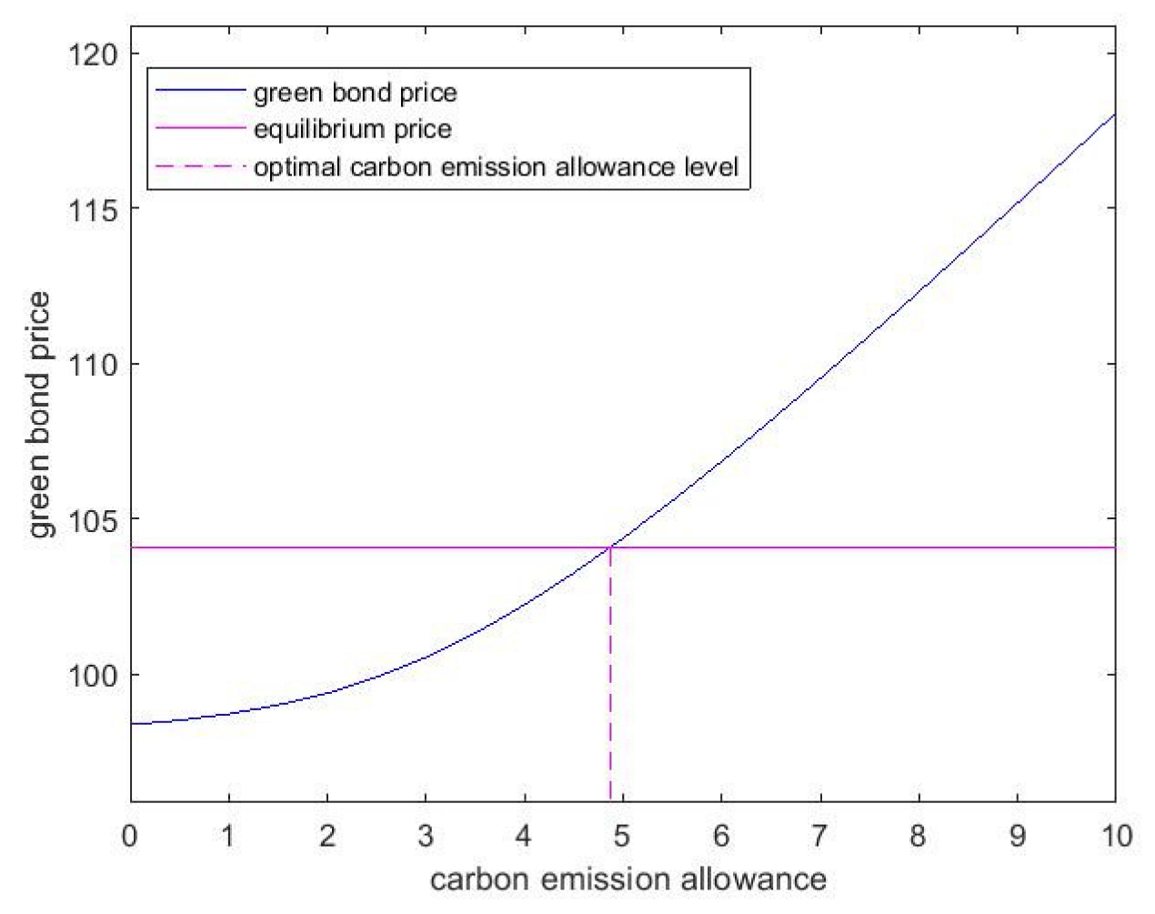
Figure 1 displays the trend of green bond price changes with the increase in carbon emission allowances from 0 to 10 units.

We can notice that (1) when the initial carbon allowance obtained by the green bond issuer is 0, the price of the green bond is only 98.38; (2) when the carbon emission allowance is at a low level, the carbon allowance and the option price are in the form of a concave function, indicating that the increase in carbon allowances has a significant stimulating effect on the price of green bonds and can encourage issuers to reduce emissions and improve their economic benefits; (3) when the government continues to issue free carbon allowances to green projects, the value of the bond price tends to rise as the sufficient allowances traded in carbon trading markets increase the income of companies, thereby increasing the expected present value of the projects and thus increasing the floating price of green bonds in the end; (4) when the carbon emission allowance hit the point of 4.88 units, then the issuer can obtain excess carbon emission reduction trading benefits so that the green bond reaches the equilibrium price of 104.11; (5) as the government continues to issue free carbon allowances to green projects, the bond price will increase linearly, indicating that the carbon allowances are relatively abundant at this time. The simulative effect of the carbon allowance policy on the price of the green bond has stabilized. Although increasing carbon allowances can further increase the price of the green bond, the issuer will reduce their enthusiasm for emission reduction, and the government will also be under too much pressure, which is unlikely to achieve the goal of optimizing public resources.

The above results may partly explain that if the government is faced with total carbon constraints, issuers cannot obtain free initial carbon emission allowances, or the carbon allowances obtained are insufficient, and thus, the green bonds will not be able to reach the equilibrium price, leading to the failure to achieve the optimal allocation of resources. If the initial carbon allowance is not constrained, the government can reasonably increase the initial carbon allowance distributed to the bond issuer to help the green bond price reach a certain equilibrium level, to solve the externality of the green bond and realize the goal of optimal allocation of resources.

2.

Introduce government subsidies

In practice, due to the large gap in carbon emissions of different green projects and the difficulty of detection, it is often difficult for the government to effectively allocate the initial carbon allowances [9]. Moreover, to encourage companies to carry out technological innovation and curb the intensity of carbon emission levels, the government usually adopts the modest tightening principle of allocating carbon allowances to high-carbon companies and forces them to fulfil their carbon emission reduction obligations [8,12]. Furthermore, many scholars have found that the carbon emission trading market is not completely efficient, and it cannot fully compensate for the positive externalities brought about by the issuance of green bonds [13,14,15]. When viewed at the national level, the United Nations Framework Convention on Climate Change (UNFCCC) usually sets a given total emission reduction target every year and strives to minimize costs through carbon emission trading. In the Paris COP 21 climate agreement of December 2015, 195 signatories pledged to limit global warming to 2 °C above pre-industrial levels [62]. Moreover, the E.U. has pledged to reduce 40% of total greenhouse gas emissions within the E.U. from 1990 levels by 2030. To achieve this, the E.U. will reduce the number of emission permits available in the European Emissions Trading System (ETS) [63]. Many institutional investors have also established coalitions such as “Climate Action 100+” to require more listed companies to reduce their carbon emissions (see http://www.climateaction100.org/ (accessed on 1 March 2023)). Therefore, the reality is that companies are usually constrained by carbon allowances and cannot obtain sufficient initial carbon allowances, so the pure carbon emission trading mechanism will lead to the inability of green bonds to reach an equilibrium price. In the context of global emission reduction, there will also be total carbon allowance constraints at the national level.

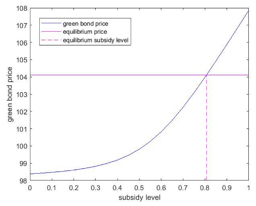
Next, we first explore how green bond prices fluctuate when the government subsidizes changes.

Figure 2 shows the changes in green bond prices without an initial carbon emission allowance. The government grants different subsidy levels to projects according to their carbon emission reductions, increasing from 0% to 100%. As we can see from Figure 2, the price of the green bond is positively correlated with the subsidy rate, and when the project with a subsidy rate of 80.7%, the price of green bonds can reach the optimal equilibrium price of 104.11.

The results shown above demonstrated that if the government does not face financial constraints, the theoretical equilibrium price of green bonds can also be reached under a certain level of subsidies. Thus, the goal of optimal allocation of public resources can be achieved. However, the more realistic situation is that some governments may face financial constraints, and some pieces of economic literature have amply proved it. For example, Bacchiocchi et al. [64] demonstrate that countries with high public debt are often fiscally constrained in investing in public goods, especially when faced with financial crises or conflicts between countries. Andersen et al. [65] state that at any given level of fiscal capacity, the government may be temporarily constrained financially, resulting in an inability to provide adequate levels of spending on public goods to meet social needs, such as spending on basic health and education services or investment in economically sound public infrastructures. They also point out that when a financially strapped government cannot raise enough money to fund its optimal level of public spending, it is likely to fill the financial gap with whatever tools are available, including participation in emissions trading. Therefore, addressing the externalities of green bonds only through government subsidies will be a big burden for the government. Green bond prices will not reach the theoretical equilibrium price if governments face fiscal constraints that prevent them from providing sufficient funds to finance the highest levels of public spending. At this point, emission trading markets based on carbon allowances will be a good choice.

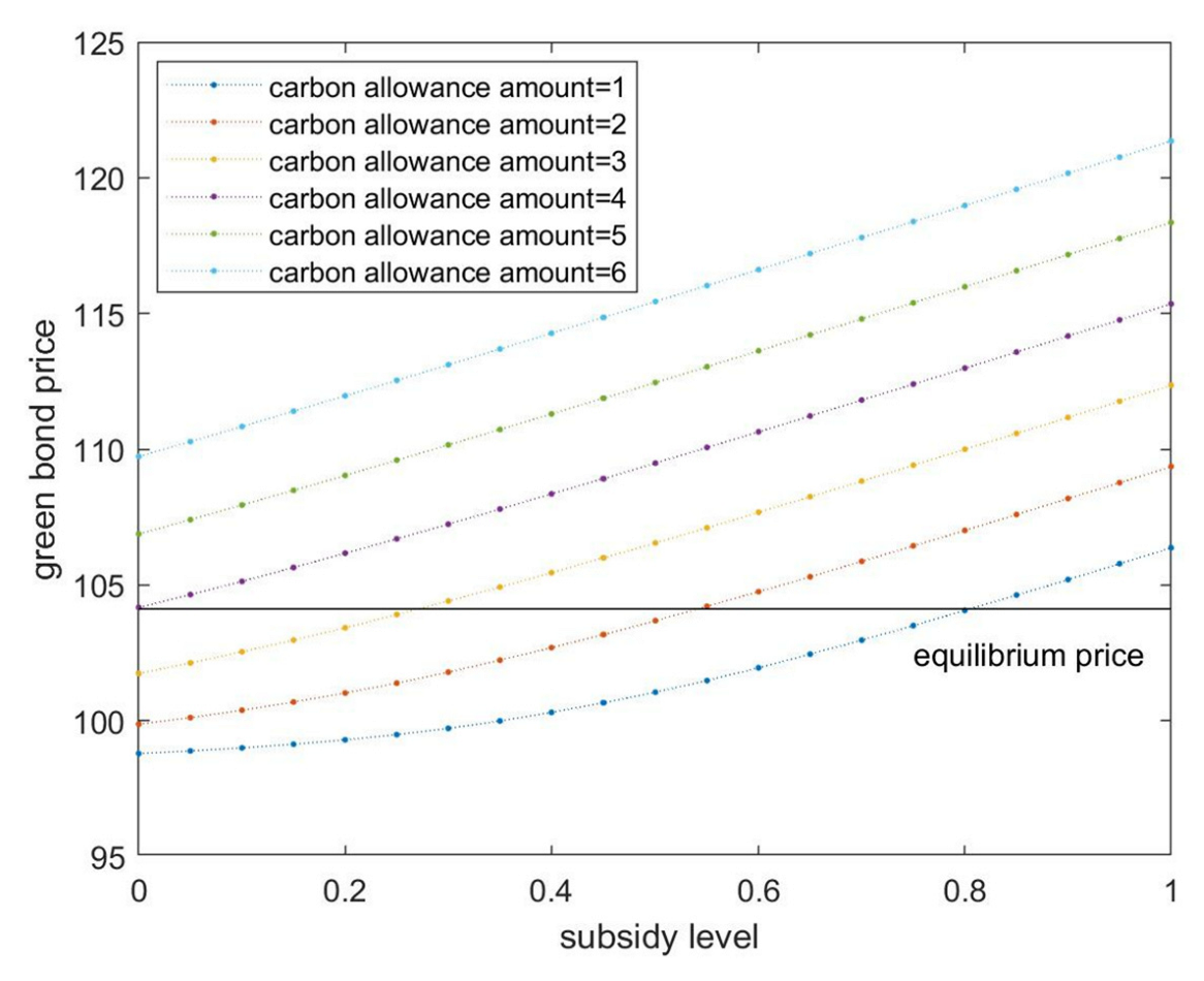
Furthermore, we analyzed the changes in green bond prices when the government is under both financial constraints and carbon allowance pressure. It is also discussed that the changes in green bond prices are under the combined effect of the carbon allowance-based carbon emission trading mechanism and government subsidies.

Figure 3 shows the changes in green bond prices when the government’s initial free carbon emission allowances range from 1 unit to 6 units. The government’s subsidy rate for the green bond-supported project based on its carbon emission reductions varies from 0% to 100%. Overall, the subsidy level comes with an increase in bond prices. With the increase in allocated carbon allowances, the relationship between the subsidy rate and the price becomes more and more linear. In addition, when the initial carbon allowance is insufficient (lower than the theoretical optimal carbon allowance of 4.88 units we calculated above), we can always find a suitable subsidy level so that the curve intersects the equilibrium price level line; and the lower the carbon allowance, the higher the subsidy level required for green bonds to reach an equilibrium price.

Figure 3 indicates that (1) when the initial carbon allowance allocated to the issuer is insufficient, government subsidies can be used as supplementary methods of carbon emission trading mechanism to assist in internalizing green bond externalities. By reasonably raising the level of government subsidies, the bond price can be brought back to the equilibrium price, and the effective allocation of public resources is realized; (2) when the bond price exceeds the equilibrium price with the increase in subsidy level, the effect of increasing the subsidy does not become obvious. Thus, excessive government subsidies will also lead to an unreasonable allocation of public resources.

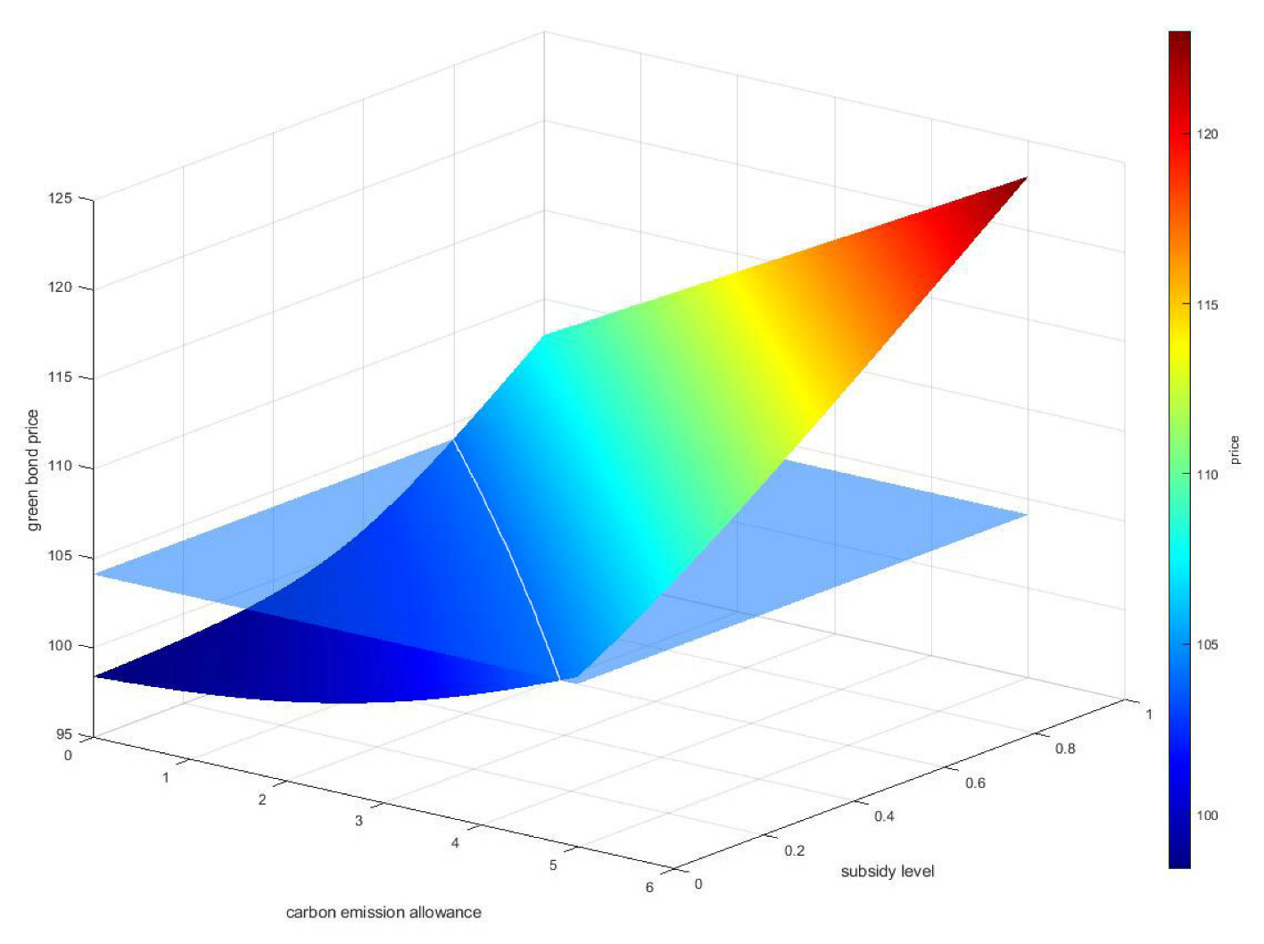
Figure 4 intuitively exhibits the relationship between the impact of carbon emission allowances and government subsidies on green bond prices. The allowances range from 0 to 5 units, and government subsidy levels range from 0% to 100%. The translucence surface is the green bond’s equilibrium price surface. The white curve formed by the intersection of the two surfaces is the combination of government subsidies and carbon emission allowances that can achieve the equilibrium price. According to Figure 4, we can see that carbon allowances and government subsidies are in a mutually substitutable relationship: (1) when the amount of carbon emission allowance is fixed, the price of the green bond is an increasing function of the government subsidy level. Therefore, in the early stage, when the initial carbon allowance allocation may be unreasonable or when the government faces carbon emission allowance constraints, and the issuer cannot obtain sufficient carbon emission allowances, the government can help the green bond price reach the equilibrium level by increasing subsidies; (2) when the government subsidy level is fixed, the bond price is positively correlated with the carbon emission allowance level, and the government can help the green bond price reach the equilibrium level by increasing initial allowances when it faces fiscal constraints and cannot provide sufficient subsidies to the issuer; (3) if the government is faced with both carbon emission allowance constraints and financial constraints, the policymaker can reasonably choose an appropriate combination strategy of allowances and subsidies according to the actual situation. Thus, the green bond price can reach the equilibrium price surface.

To summarize, the carbon emission trading mechanism based on carbon emission allowances combining government subsidies can effectively solve the externality of green bonds. When the government faces both carbon allowance constraints and financial constraints, policymakers can reasonably control the allocation of carbon allowances allocated to green bond issuers according to governments’ conditions to solve the externalities of green bonds. Thus, green bonds can achieve the theoretical equilibrium price, thereby reducing the cost of issuing green bonds and realizing the optimal allocation of public resources.

3.3. Sensitivity Analysis

In this paper, we concentrate on two main factors that affect green bond prices most to conduct the sensitivity analysis. The first one is the volatility of carbon emission prices. Since we select the carbon emission price as the underlying price of green projects supported by green bonds, the volatility of carbon emission price is one of the most important factors affecting the value of green bonds: the higher the volatility of carbon emission prices, the greater the uncertainty of green bond prices. Another factor considered is the fixed investment cost during the implementation of green bond-supported projects. Since the projects are mainly environmentally friendly projects, the fixed investment cost of the project and the investment cost of facilities related to emission reduction technologies will impact the options price. Intuitively speaking, if a project has more fixed costs, the investment cost of emission reduction technology will be relatively less, which would influence green bond prices to some extent.

In what follows, we perform the numerical computation to show how the volatility of carbon emission prices and the size of fixed costs jointly influence the impact of green bond prices.

Figure 5 displays how green bond prices change with the carbon price volatility increasing from 10% to 50% with a gradient of 5%, and the fixed cost increases from 0 to 5 with a gradient of 0.5 when there are no carbon allowances and government subsidies. Not surprisingly, Figure 5 indicates that (1) with all other conditions equal, the green bond price increases with the increase in carbon emission price volatility, reflecting the value attributed to the uncertainty of the project value; (2) the green bond price is a decreasing function of the project’s fixed cost, and this may, at least partly, explain why companies should invest more in carbon emission-related technologies.

Next, we separately examine the impact of volatility and fixed costs on bond prices.

Figure 6 shows the trend of bond prices as a function of the subsidy level when volatility varies from 10% to 50% in a 10% gradient. As the volatility increases, the bond price also increases. Another phenomenon is that the impact of the volatility change on the bond price shrinks with the increase in the subsidy level, which shows that increasing the subsidy level for green bonds will weaken the impact of carbon emission price uncertainty on bond prices.

Finally, Figure 7 shows the changing trend of green bond prices with the subsidy level when the fixed cost varies from 0 to 5 units. We can find that as the fixed cost increases, the green bond price decreases, indicating that the more the project spends on fixed costs that are not related to emission reduction technologies, the lower the bond price.

4. Discussion

From the perspective of green bond externalities, this paper constructs a pricing model incorporating both the carbon emission trading mechanism and government subsidies to solve the externalities of issuing green bonds. We derive an approximate expression for green bond prices and study the coordination mechanism between allowances and subsidies. As green bonds may face sudden environmental shocks and policy shocks, the value of green bonds is divided into the fixed income part and floating value part to separately assess green bond prices. Under the real options framework, the green bond pricing model comprising environmental risk is proposed from the FBM with double exponential jumps model. The expression is derived from the fast Fourier transform method. Based on the pricing model above, we investigate the influence of different factors on green bond prices. We further discuss the optimal strategy the government has taken in different situations and constraints, referring to carbon emission allowances and government subsidies to meet the equilibrium price of green bonds at which the externalities are internalized.

Our numerical simulation results indicate that (1) when governments are faced with the amount of carbon emission constraints but can still provide sufficient carbon emission allowances, the carbon emission trading mechanism could be introduced to help green projects supported by green bonds receive extra financial incentives from carbon emission trading markets, leading to green bonds reaching the ideal equilibrium price under the conditions of optimal allocation of public resources; (2) when governments are faced with the amount of carbon emission constraints, and cannot issue sufficient carbon allowances to green bond issuers, government subsidies could be introduced to reduce green project investment costs supported by green bonds so that green bonds can achieve the equilibrium price; (3) when governments are faced with both the financial constraints and the amount of carbon emissions constraints, policymakers can reasonably control the allocation between carbon allowances and government subsidies according to the governments’ situation to solve externalities of green bonds. The results presented in this paper have provided valuable insights into the impact of the combination of government policies and carbon emission trading mechanisms on green bond pricing, along with the optimal carbon emission allowance and government subsidy level under different situations. In this way, the green bond could reach the equilibrium price under the optimal allocation of public resources, and the positive externality of issuing green bonds could be solved to some extent. However, the simulation results are idealistic, and can be extended in several aspects in future work. In our paper, the equilibrium price of green bonds when public resources are optimally allocated is given exogenously, so we can empirically explore the equilibrium price of green bonds based on the actual green bond market in the future. Furthermore, we mainly focus on risks related to carbon price and have not considered default risk for simplicity. In addition, the coordinating analyses between carbon emission allowances and subsidies in this paper merely involve a situation for a single green bond issuer. To further study, we will consider more factors such as the situation of multiple issuers and the default risks when the green bond market is entering a more mature stage in the future. The carbon emission trading mechanism and government subsidies, the carbon emission tax, and other environmental policy tools could be further discussed together to solve the externality of green bonds and, as our paper highlights, promote the optimal allocation of public resources and social welfare.

References

- Karpf, A.; Mandel, A. The changing value of the ‘green’ label on the US municipal bond market. Nat. Clim. Change 2018, 8, 161–165. [Google Scholar] [CrossRef]
- Louche, C.; Busch, T.; Crifo, P.; Marcus, A. Financial markets and the transition to a low-carbon economy: Challenging the dominant logics. Organ. Environ. 2019, 32, 3–17. [Google Scholar] [CrossRef]
- Flammer, C. Corporate green bonds. J. Financ. Econ. 2021, 142, 499–516. [Google Scholar] [CrossRef]
- Bartram, S.M.; Hou, K.; Kim, S. Real effects of climate policy: Financial constraints and spillovers. J. Financ. Econ. 2022, 143, 668–696. [Google Scholar] [CrossRef]
- Agliardi, E.; Agliardi, R. Pricing climate-related risks in the bond market. J. Financ. Stab. 2021, 54, 100868. [Google Scholar] [CrossRef]
- Jaffe, A.B.; Newell, R.G.; Stavins, R.N. Environmental policy and technological change. Environ. Resour. Econ. 2002, 22, 41–70. [Google Scholar] [CrossRef]
- Ghisetti, C.; Pontoni, F. Investigating policy and R&D effects on environmental innovation: A meta-analysis. Ecol. Econ. 2015, 118, 57–66. [Google Scholar]
- Jotzo, F.; Karplus, V.; Grubb, M.; Löschel, A.; Neuhoff, K.; Wu, L.; Teng, F. China’s emissions trading takes steps towards big ambitions. Nat. Clim. Change 2018, 8, 265–267. [Google Scholar] [CrossRef]
- Wang, B.; Ji, F.; Zheng, J.; Xie, K.; Feng, Z. Carbon emission reduction of coal-fired power supply chain enterprises under the revenue sharing contract: Perspective of coordination game. Energy Econ. 2021, 102, 105467. [Google Scholar] [CrossRef]
- Heine, D.; Semmler, W.; Mazzucato, M.; Braga, J.P.; Flaherty, M.; Gevorkyan, A.; Hayde, E.; Radpour, S. Financing low-carbon transitions through carbon pricing and green bonds. Vierteljahrsh. Zur Wirtsch. 2019, 88, 29–49. [Google Scholar] [CrossRef]
- Wang, W.; Zhang, Y.-J. Does China’s carbon emissions trading scheme affect the market power of high-carbon enterprises? Energy Econ. 2022, 108, 105906. [Google Scholar] [CrossRef]
- Zhang, Y.-J.; Wang, W. How does China’s carbon emissions trading (CET) policy affect the investment of CET-covered enterprises? Energy Econ. 2021, 98, 105224. [Google Scholar] [CrossRef]
- Charles, A.; Darné, O.; Fouilloux, J. Market efficiency in the European carbon markets. Energy Policy 2013, 60, 785–792. [Google Scholar] [CrossRef]
- Feng, Z.-H.; Zou, L.-L.; Wei, Y.-M. Carbon price volatility: Evidence from EU ETS. Appl. Energy 2011, 88, 590–598. [Google Scholar] [CrossRef]
- Wang, X.-Q.; Su, C.-W.; Lobonţ, O.-R.; Li, H.; Nicoleta-Claudia, M. Is China’s carbon trading market efficient? Evidence from emissions trading scheme pilots. Energy 2022, 245, 123240. [Google Scholar] [CrossRef]
- Saravade, V.; Chen, X.; Weber, O.; Song, X. Impact of regulatory policies on green bond issuances in China: Policy lessons from a top-down approach. Clim. Policy 2023, 23, 96–107. [Google Scholar] [CrossRef]
- Abrell, J.; Kosch, M.; Rausch, S. Carbon abatement with renewables: Evaluating wind and solar subsidies in Germany and Spain. J. Public Econ. 2019, 169, 172–202. [Google Scholar] [CrossRef]
- Bialek, S.; Unel, B. Efficiency in wholesale electricity markets: On the role of externalities and subsidies. Energy Econ. 2022, 109, 105923. [Google Scholar] [CrossRef]
- Tolliver, C.; Keeley, A.R.; Managi, S. Policy targets behind green bonds for renewable energy: Do climate commitments matter? Technol. Forecast. Soc. Change 2020, 157, 120051. [Google Scholar] [CrossRef]
- Xu, L.; Wang, C.; Miao, Z.; Chen, J. Governmental subsidy policies and supply chain decisions with carbon emission limit and consumer’s environmental awareness. RAIRO-Oper. Res. 2019, 53, 1675–1689. [Google Scholar] [CrossRef]
- Li, Y.; Deng, Q.; Zhou, C.; Feng, L. Environmental governance strategies in a two-echelon supply chain with tax and subsidy interactions. Ann. Oper. Res. 2020, 290, 439–462. [Google Scholar] [CrossRef]
- Uddin, G.S.; Jayasekera, R.; Park, D.; Luo, T.; Tian, S. Go green or stay black: Bond market dynamics in Asia. Int. Rev. Financ. Anal. 2022, 81, 102114. [Google Scholar] [CrossRef]
- Keeley, A.R.; Matsumoto, K.i. Relative significance of determinants of foreign direct investment in wind and solar energy in developing countries–AHP analysis. Energy Policy 2018, 123, 337–348. [Google Scholar] [CrossRef]
- Huang, W.; Zhou, W.; Chen, J.; Chen, X. The government’s optimal subsidy scheme under Manufacturers’ competition of price and product energy efficiency. Omega 2019, 84, 70–101. [Google Scholar] [CrossRef]
- Taghizadeh-Hesary, F.; Yoshino, N. The way to induce private participation in green finance and investment. Financ. Res. Lett. 2019, 31, 98–103. [Google Scholar] [CrossRef]
- Wang, J.; Chen, X.; Li, X.; Yu, J.; Zhong, R. The market reaction to green bond issuance: Evidence from China. Pac.-Basin Financ. J. 2020, 60, 101294. [Google Scholar] [CrossRef]
- Agliardi, E.; Agliardi, R. Financing environmentally-sustainable projects with green bonds. Environ. Dev. Econ. 2019, 24, 608–623. [Google Scholar] [CrossRef]
- Ehlers, T.; Packer, F. Green Bonds–certification, shades of green and environmental risks. Bank Int. Settl. 2016. Available online: https://unepinquiry.org/wp-content/uploads/2016/09/12_Green_Bonds_Certification_Shades_of_Green_and_Environmental_Risks.pdf (accessed on 1 March 2023).
- Seltzer, L.; Starks, L.T.; Zhu, Q. Climate Regulatory Risks and Corporate Bonds; Nanyang Business School Research Paper; NBER: Cambridge, MA, USA, 2020. [Google Scholar]
- Krueger, P.; Sautner, Z.; Starks, L.T. The importance of climate risks for institutional investors. Rev. Financ. Stud. 2020, 33, 1067–1111. [Google Scholar] [CrossRef]
- Karydas, C.; Xepapadeas, A. Pricing climate change risks: CAPM with rare disasters and stochastic probabilities. CER-ETH Work. Pap. Ser. Work. Pap. 2019, 19, 311. [Google Scholar] [CrossRef]
- Li, X.; Li, Z.; Su, C.-W.; Umar, M.; Shao, X. Exploring the asymmetric impact of economic policy uncertainty on China’s carbon emissions trading market price: Do different types of uncertainty matter? Technol. Forecast. Soc. Change 2022, 178, 121601. [Google Scholar] [CrossRef]
- Yu, J.; Zhang, M.; Liu, R.; Wang, G. Dynamic Effects of Climate Policy Uncertainty on Green Bond Volatility: An Empirical Investigation Based on TVP-VAR Models. Sustainability 2023, 15, 1692. [Google Scholar] [CrossRef]
- Li, H.; Li, Q.; Huang, X.; Guo, L. Do green bonds and economic policy uncertainty matter for a carbon price? New insights from a TVP-VAR framework. Int. Rev. Financ. Anal. 2023, 86, 102502. [Google Scholar] [CrossRef]
- Myers, S.C. Determinants of corporate borrowing. J. Financ. Econ. 1977, 5, 147–175. [Google Scholar] [CrossRef]
- Mason, S.P.; Merton, R.C. The role of contingent claims analysis in corporate finance. In World Scientific Reference on Contingent Claims Analysis in Corporate Finance: Volume 1: Foundations of CCA and Equity Valuation; World Scientific: Singapore, 2019; pp. 123–168. [Google Scholar]
- Lambrecht, B.M. Real options in finance. J. Bank. Financ. 2017, 81, 166–171. [Google Scholar] [CrossRef]
- Anda, J.; Golub, A.; Strukova, E. Economics of climate change under uncertainty: Benefits of flexibility. Energy Policy 2009, 37, 1345–1355. [Google Scholar] [CrossRef]
- Marzouk, M.; Ali, M. Mitigating risks in wastewater treatment plant PPPs using minimum revenue guarantee and real options. Util. Policy 2018, 53, 121–133. [Google Scholar] [CrossRef]
- Yao, X.; Fan, Y.; Zhu, L.; Zhang, X. Optimization of dynamic incentive for the deployment of carbon dioxide removal technology: A nonlinear dynamic approach combined with real options. Energy Econ. 2020, 86, 104643. [Google Scholar] [CrossRef]
- Zhang, S.; Yang, Z.; Wang, S. Design of green bonds by double-barrier options. Discret. Contin. Dyn. Syst.-S 2020, 13, 1867. [Google Scholar] [CrossRef]
- Xiang, S.; Cao, Y. Green finance and natural resources commodities prices: Evidence from COVID-19 period. Resour. Policy 2023, 80, 103200. [Google Scholar] [CrossRef]
- De Angelis, T.; Tankov, P.; Zerbib, O.D. Environmental impact investing. SSRN 2020, 3562534. [Google Scholar] [CrossRef]
- Eichholtz, P.; Holtermans, R.; Kok, N.; Yönder, E. Environmental performance and the cost of debt: Evidence from commercial mortgages and REIT bonds. J. Bank. Financ. 2019, 102, 19–32. [Google Scholar] [CrossRef]
- Metcalf, G.E. An emissions assurance mechanism: Adding environmental certainty to a US carbon tax. Rev. Environ. Econ. Policy 2020, 14, 114–130. [Google Scholar] [CrossRef]
- Pan, D.; Zhang, C.; Zhu, D.; Ji, Y.; Cao, W. A novel method of detecting carbon asset price jump characteristics based on significant information shocks. Financ. Res. Lett. 2022, 47, 102626. [Google Scholar] [CrossRef]
- Barro, R.J.; Liao, G.Y. Rare disaster probability and options pricing. J. Financ. Econ. 2021, 139, 750–769. [Google Scholar] [CrossRef]
- Frunza, M.-C.; Guegan, D. Derivative Pricing and Hedging on Carbon Market. CES Working Papers. 2010. Available online: https://shs.hal.science/halshs-00461474 (accessed on 1 March 2023).
- Zhou, K.; Li, Y. Influencing factors and fluctuation characteristics of China’s carbon emission trading price. Phys. A Stat. Mech. Its Appl. 2019, 524, 459–474. [Google Scholar] [CrossRef]
- Zou, S.; Zhang, T. Multifractal detrended cross-correlation analysis of the relation between price and volume in European carbon futures markets. Phys. A Stat. Mech. Its Appl. 2020, 537, 122310. [Google Scholar] [CrossRef]
- Liu, Z.; Huang, S. Carbon option price forecasting based on modified fractional Brownian motion optimized by GARCH model in carbon emission trading. N. Am. J. Econ. Financ. 2021, 55, 101307. [Google Scholar] [CrossRef]
- Aslam, F.; Ali, I.; Amjad, F.; Ali, H.; Irfan, I. On the inner dynamics between Fossil fuels and the carbon market: A combination of seasonal-trend decomposition and multifractal cross-correlation analysis. Environ. Sci. Pollut. Res. 2023, 30, 25873–25891. [Google Scholar] [CrossRef]
- Tang, A.; Chiara, N.; Taylor, J.E. Financing renewable energy infrastructure: Formulation, pricing and impact of a carbon revenue bond. Energy Policy 2012, 45, 691–703. [Google Scholar] [CrossRef]
- Chevallier, J.; Sévi, B. On the stochastic properties of carbon futures prices. Environ. Resour. Econ. 2014, 58, 127–153. [Google Scholar] [CrossRef]
- Merton, R.C. Option pricing when underlying stock returns are discontinuous. J. Financ. Econ. 1976, 3, 125–144. [Google Scholar] [CrossRef]
- Jarrow, R.A.; Turnbull, S.M. Pricing derivatives on financial securities subject to credit risk. J. Financ. 1995, 50, 53–85. [Google Scholar] [CrossRef]
- Kou, S.G. A jump-diffusion model for option pricing. Manag. Sci. 2002, 48, 1086–1101. [Google Scholar] [CrossRef]
- Carr, P.; Madan, D. Option valuation using the fast Fourier transform. J. Comput. Financ. 1999, 2, 61–73. [Google Scholar] [CrossRef]
- Zhylyevskyy, O. A fast Fourier transform technique for pricing American options under stochastic volatility. Rev. Deriv. Res. 2010, 13, 1–24. [Google Scholar] [CrossRef]
- Huang, J.; Zhu, W.; Ruan, X. Option pricing using the fast Fourier transform under the double exponential jump model with stochastic volatility and stochastic intensity. J. Comput. Appl. Math. 2014, 263, 152–159. [Google Scholar] [CrossRef]
- Park, Y.-H. The effects of asymmetric volatility and jumps on the pricing of VIX derivatives. J. Econom. 2016, 192, 313–328. [Google Scholar] [CrossRef]
- UNFCCC, D. 1/CP. 21, adoption of the Paris Agreement. In Proceedings of the Report of the Conference of the Parties on Its Twenty-First Session, Paris, France, 30 November–13 December 2015.
- IPCC. Climate Change 2014: Mitigation of Climate Change; Working Group III Contribution to the Fifth Assessment Report of the Intergovernmental Panel on Climate Change; IPCC: Geneva, Switzerland, 2014. [Google Scholar]
- Bacchiocchi, E.; Borghi, E.; Missale, A. Public investment under fiscal constraints. Fisc. Stud. 2011, 32, 11–42. [Google Scholar] [CrossRef]
- Andersen, J.J.; Greaker, M. Emission trading with fiscal externalities: The case for a common carbon tax for the non-ETS emissions in the EU. Environ. Resour. Econ. 2018, 71, 803–823. [Google Scholar] [CrossRef]
Figure 1.
The equilibrium price of the green bond under optimal carbon emission allowance level.
Figure 2.
The green bond prices with subsidy levels from 0% to 100% and with 0 initial carbon allowance. The equilibrium price and the corresponding equilibrium subsidy level are also shown in the legend.
Figure 3.
The green bond prices with subsidy levels from 0% to 100% under different carbon allowances.
Figure 4.
Relations among subsidy level, carbon emission allowance, and green bond price.
Figure 5.
Green bond prices with different volatilities and fixed costs.
Figure 6.
Relationship between green bond price and subsidy levels under different volatilities.
Figure 7.
Relationship between green bond price and subsidy levels under different levels of fixed costs.