
Pavement Distress Identification Based on Computer Vision and Controller Area Network (CAN) Sensor Models
 , , and
Abstract
:1. Introduction
2. Literature Review
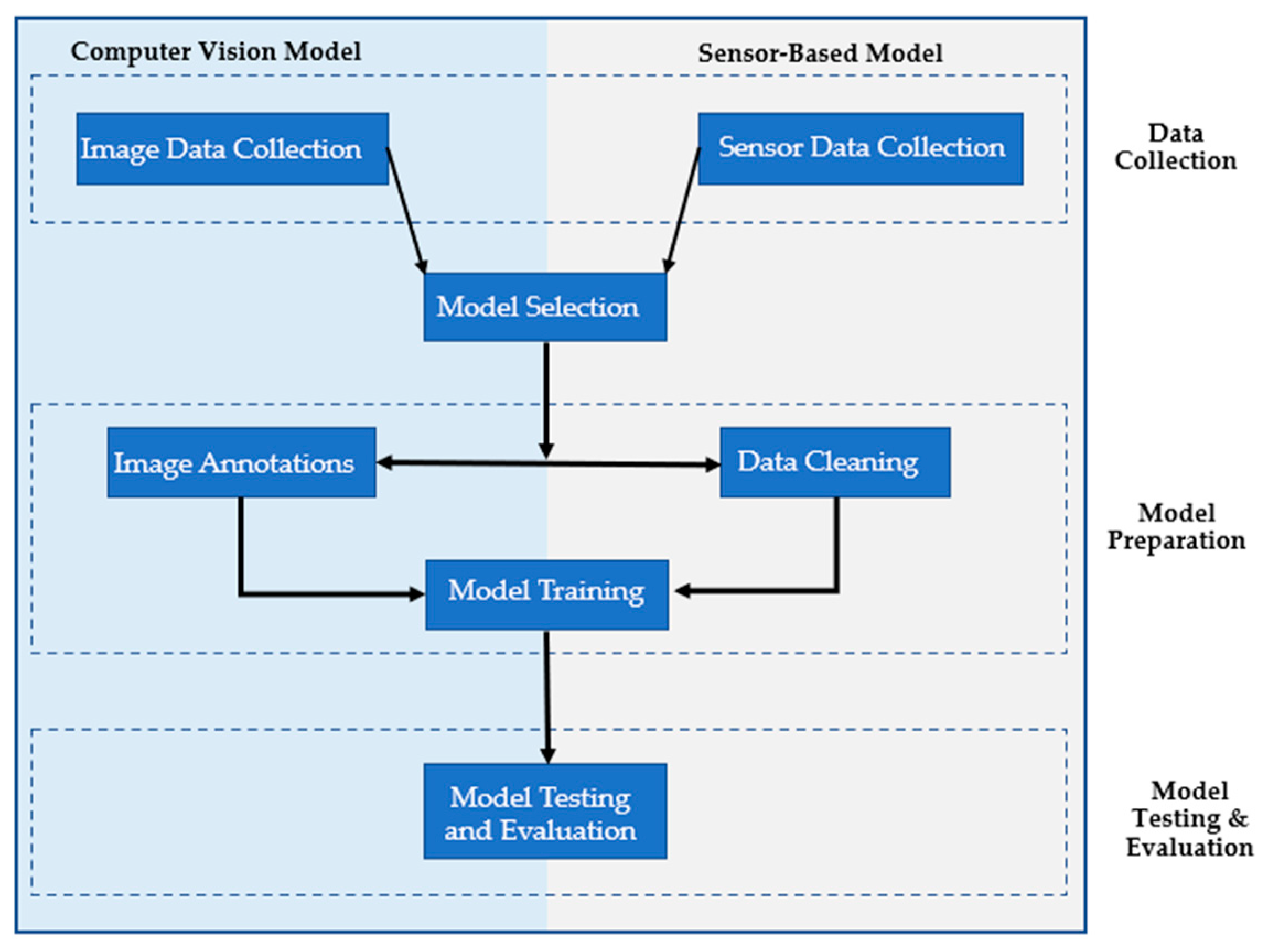
3. Methodology
3.1. Data Collection
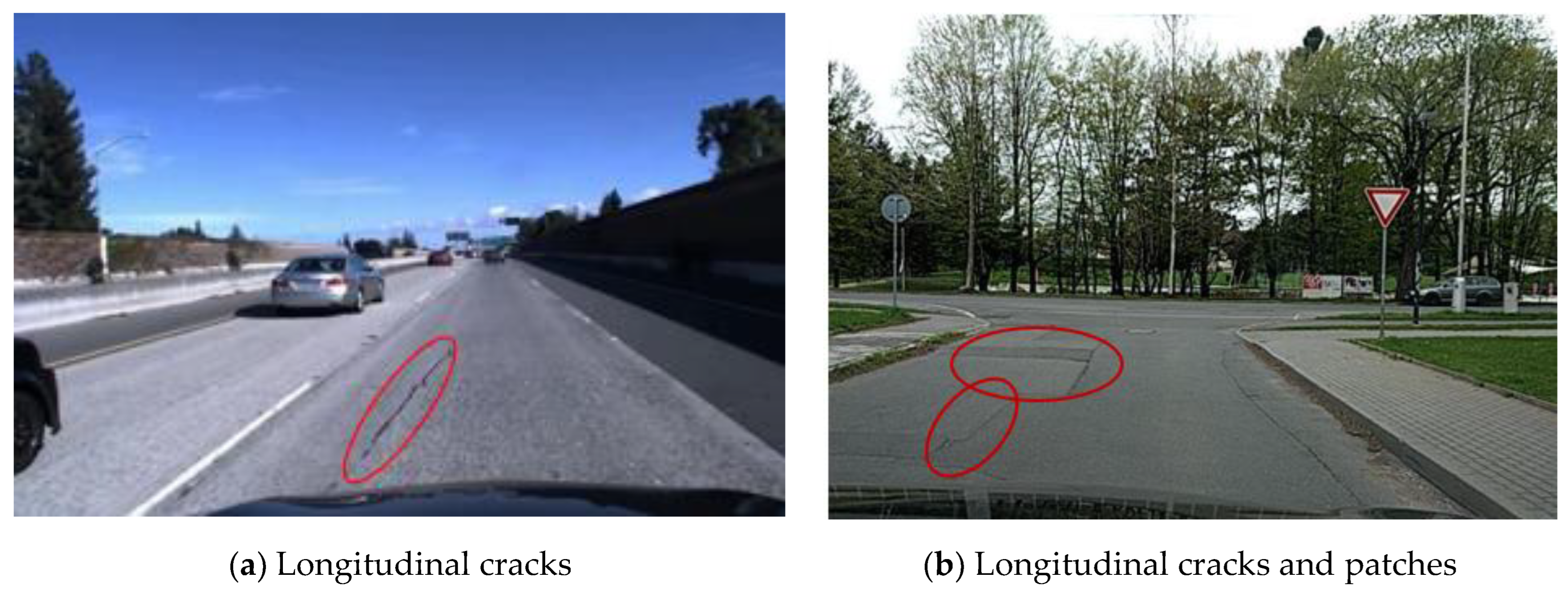
3.1.1. Vision-Based Data
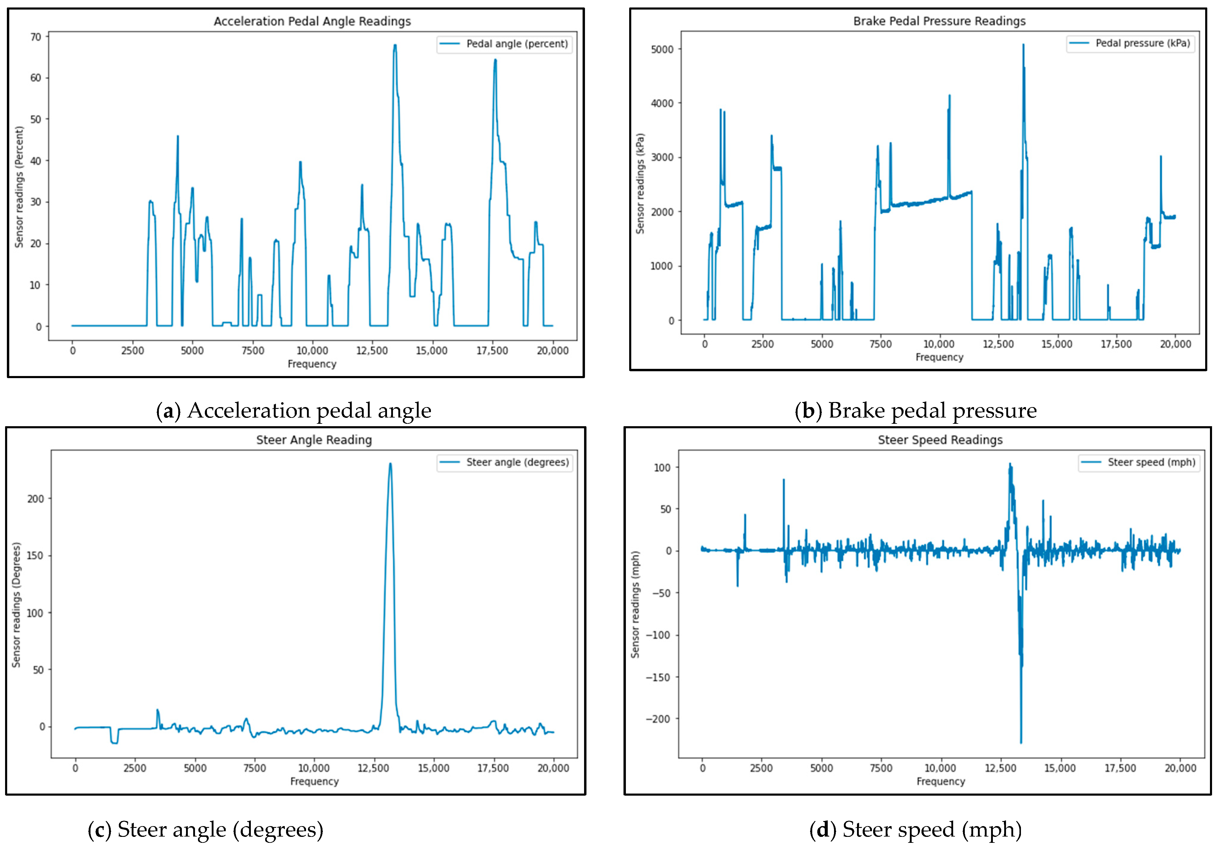
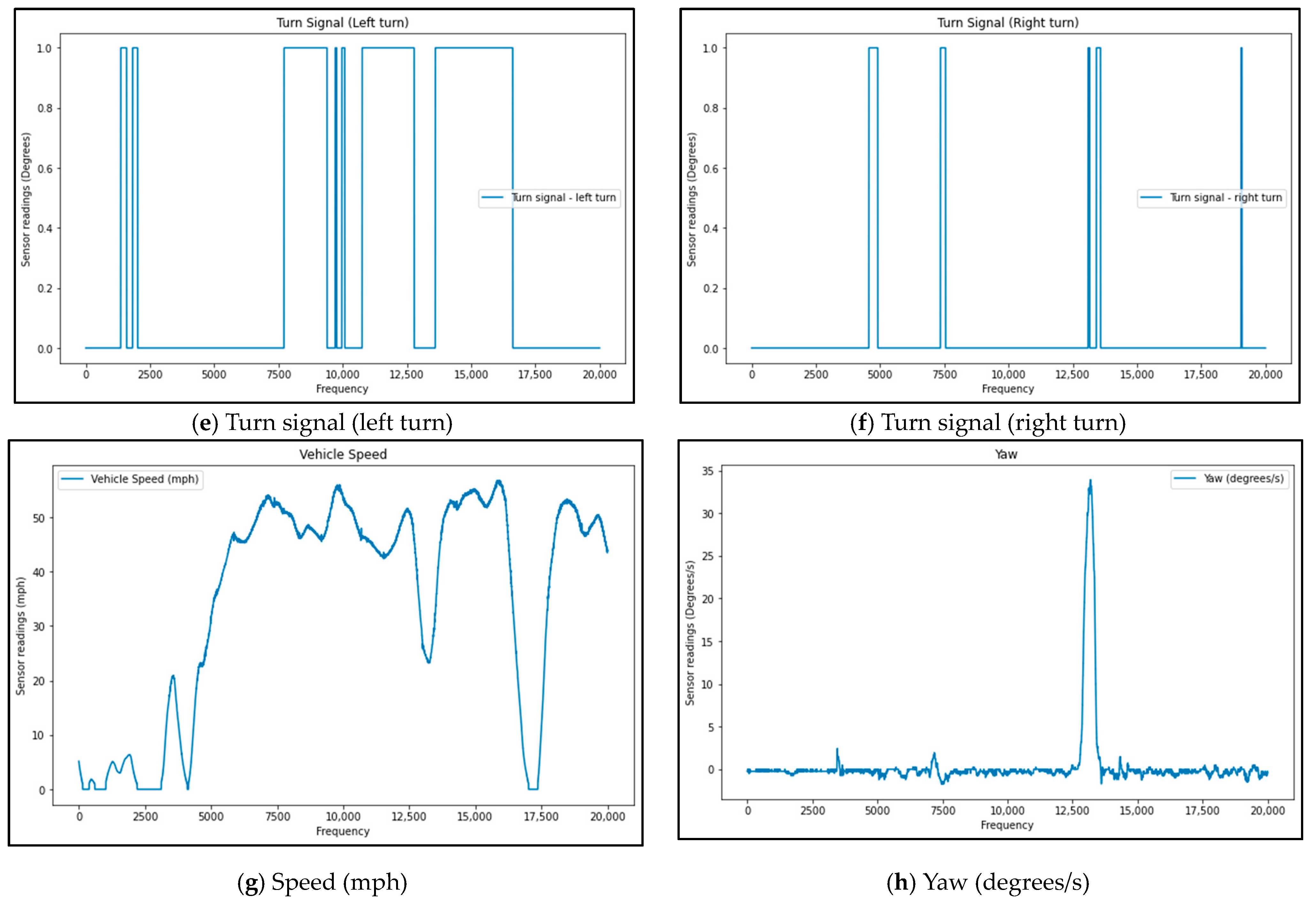
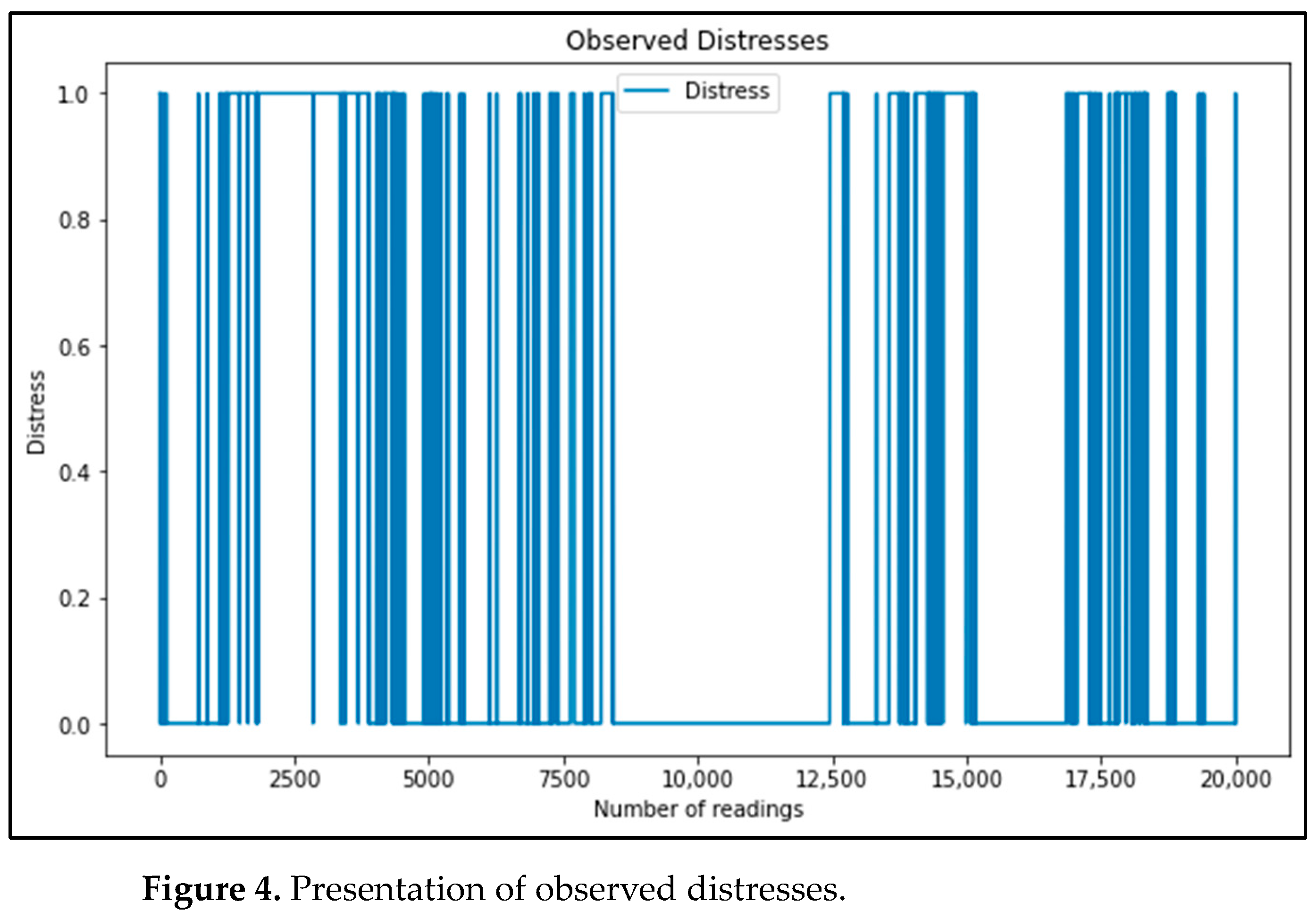
3.1.2. Sensor-Based Data
Videos
Sensors
3.2. Model Selection
3.2.1. Vision-Based Model
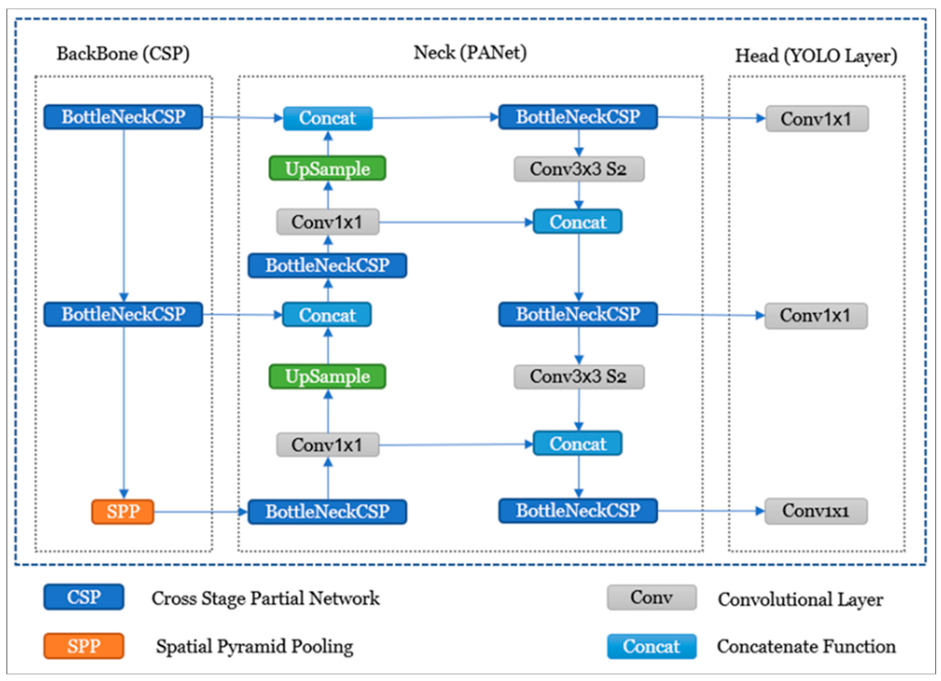
Yolov5 Architecture
Distress Classification
3.2.2. Sensor-Based Model
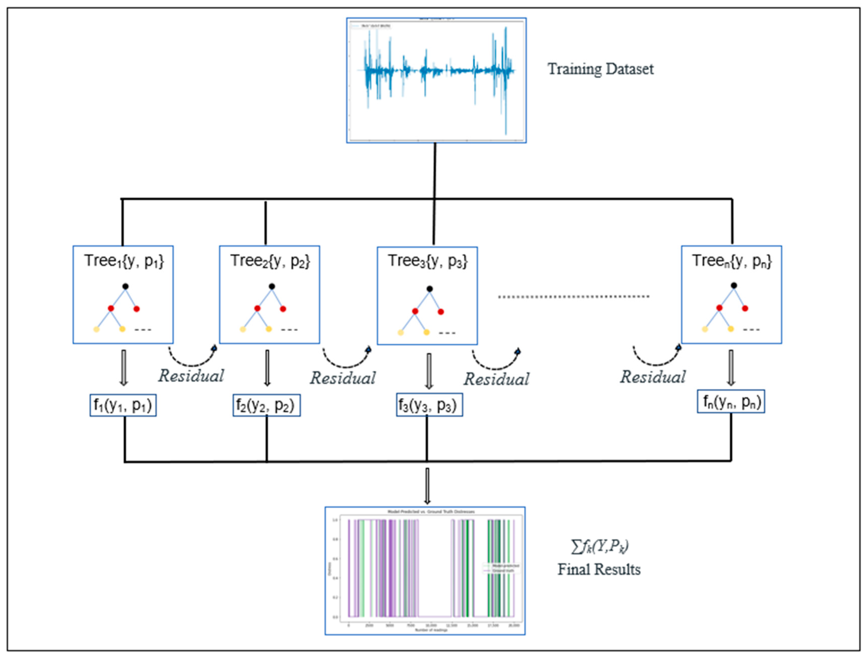
XGBoost Model Architecture
- (i)
- Decision Tree
- (ii)
- Boosting
3.3. Model Training
3.3.1. Vision-Based Model
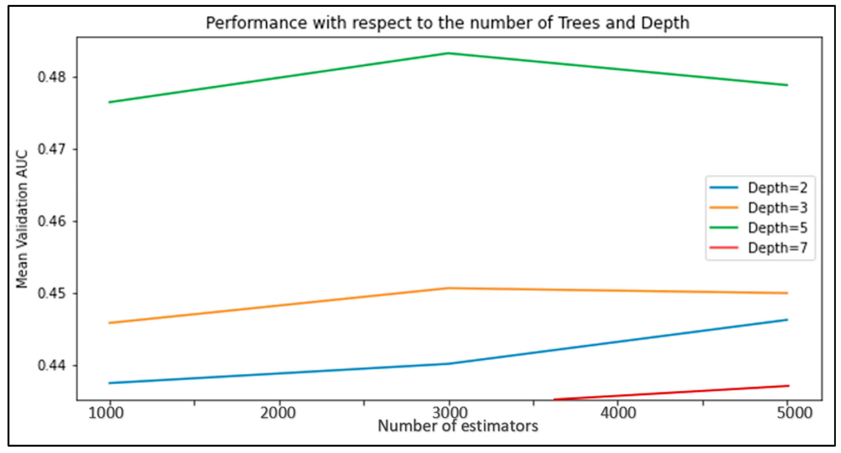
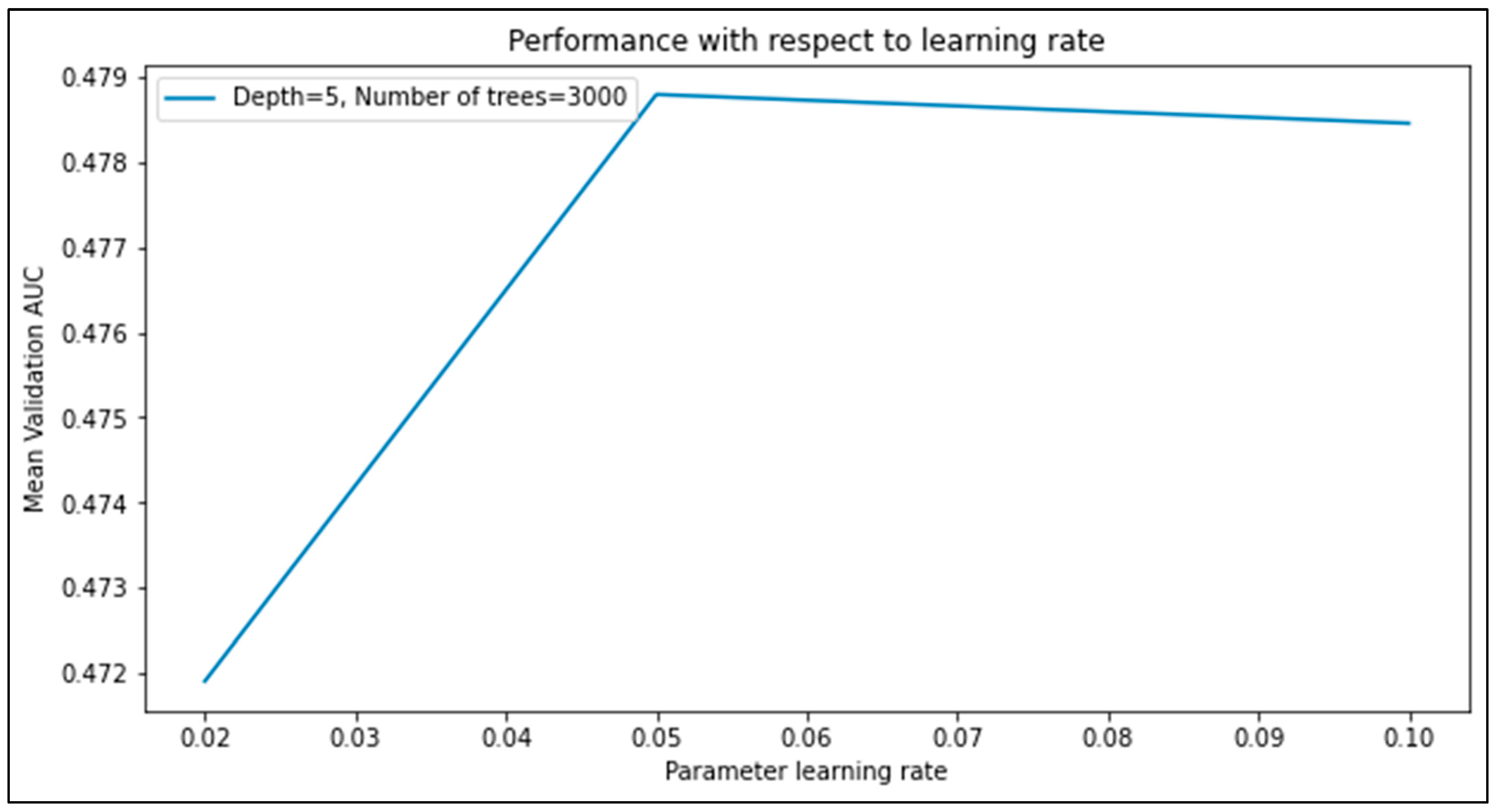
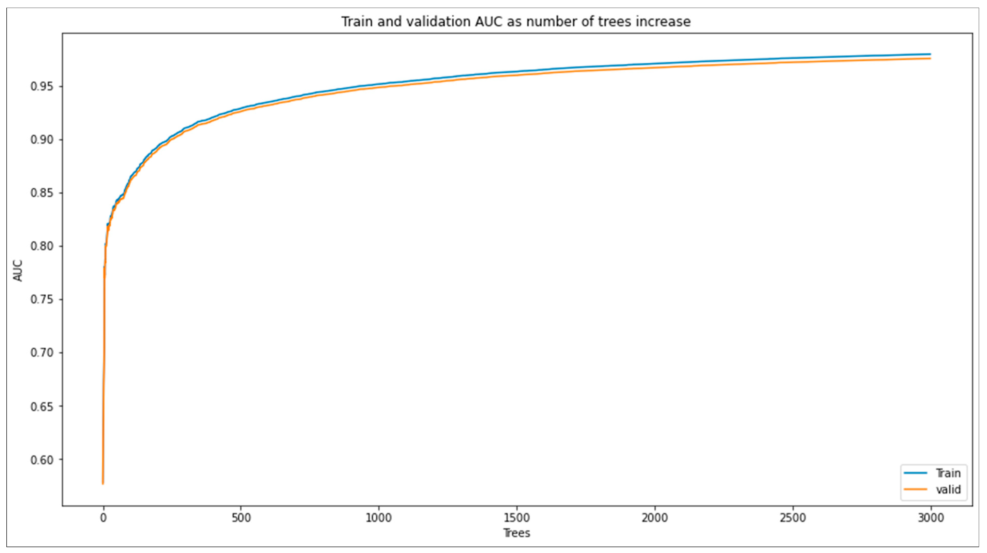
3.3.2. Sensor-Based Model
3.4. Performance Metrics
3.4.1. Vision-Based Model
3.4.2. Sensor-Based Model
Metrics
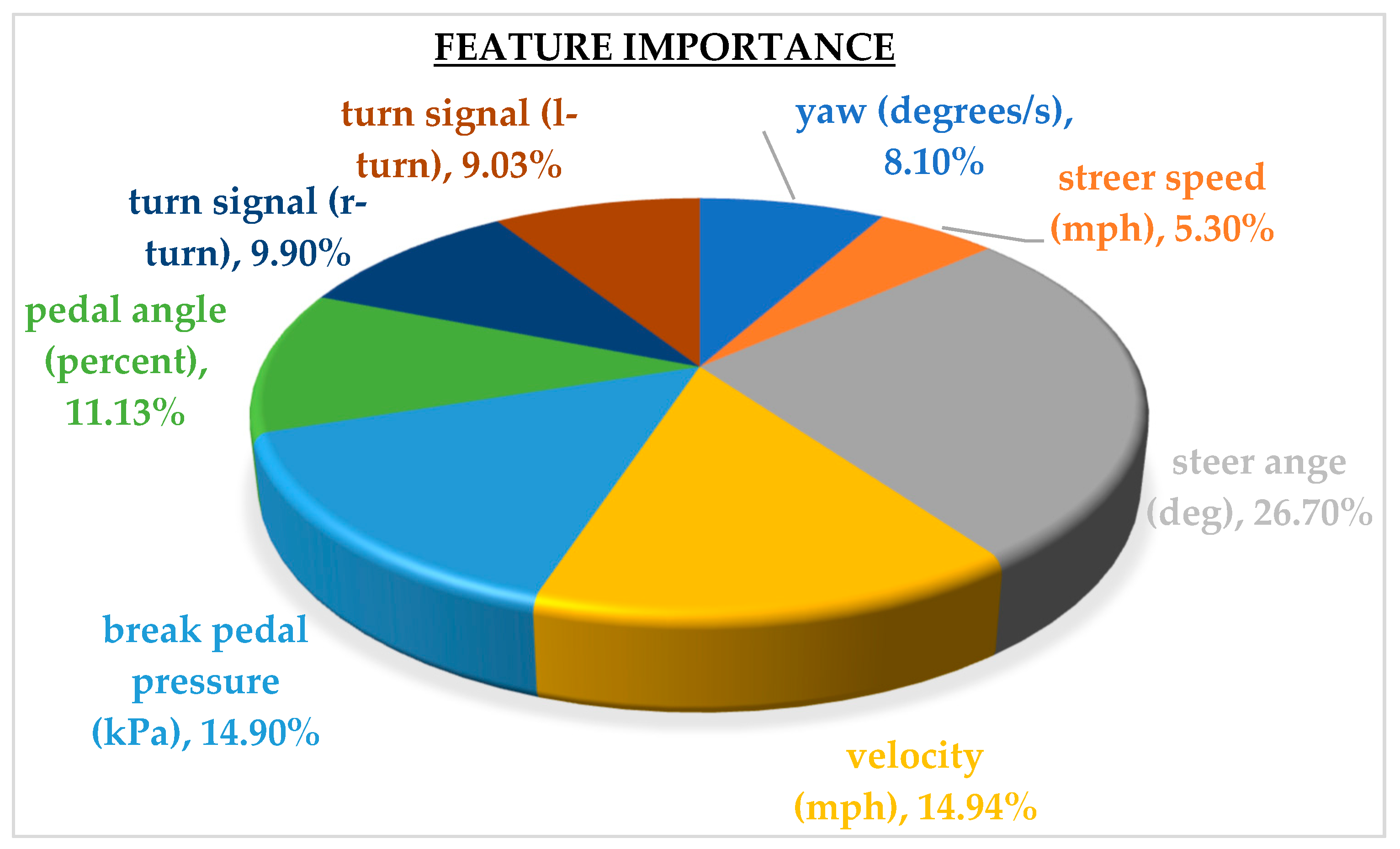
Feature Importance Assessment
3.5. Results and Analysis
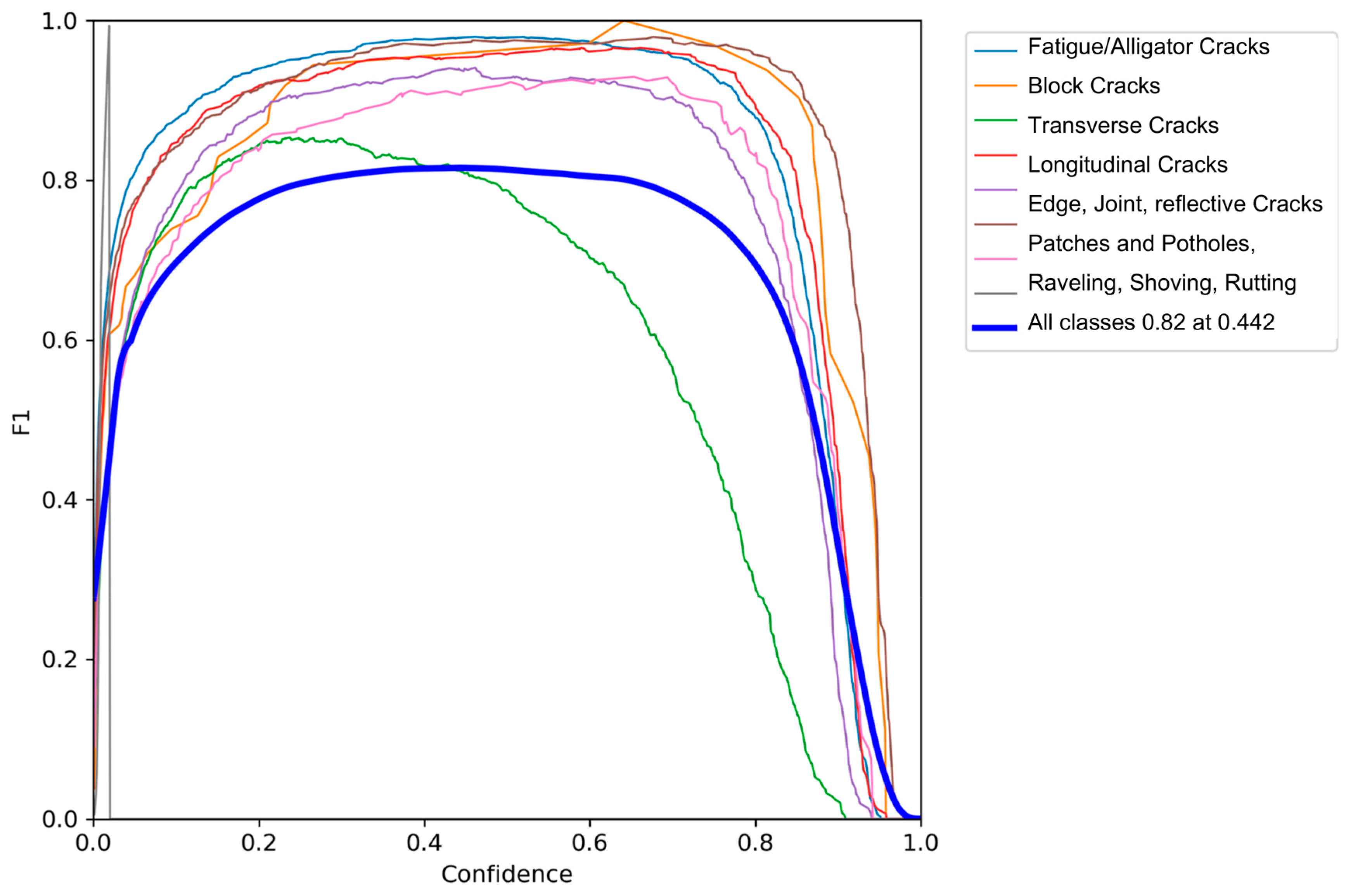
3.5.1. Results of Vision-based Road Surface Detection Model
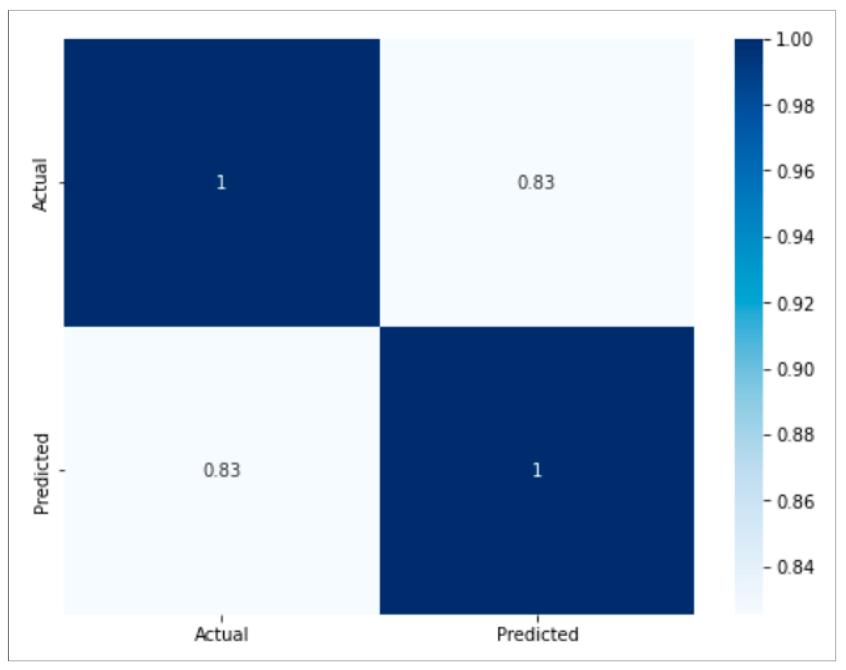
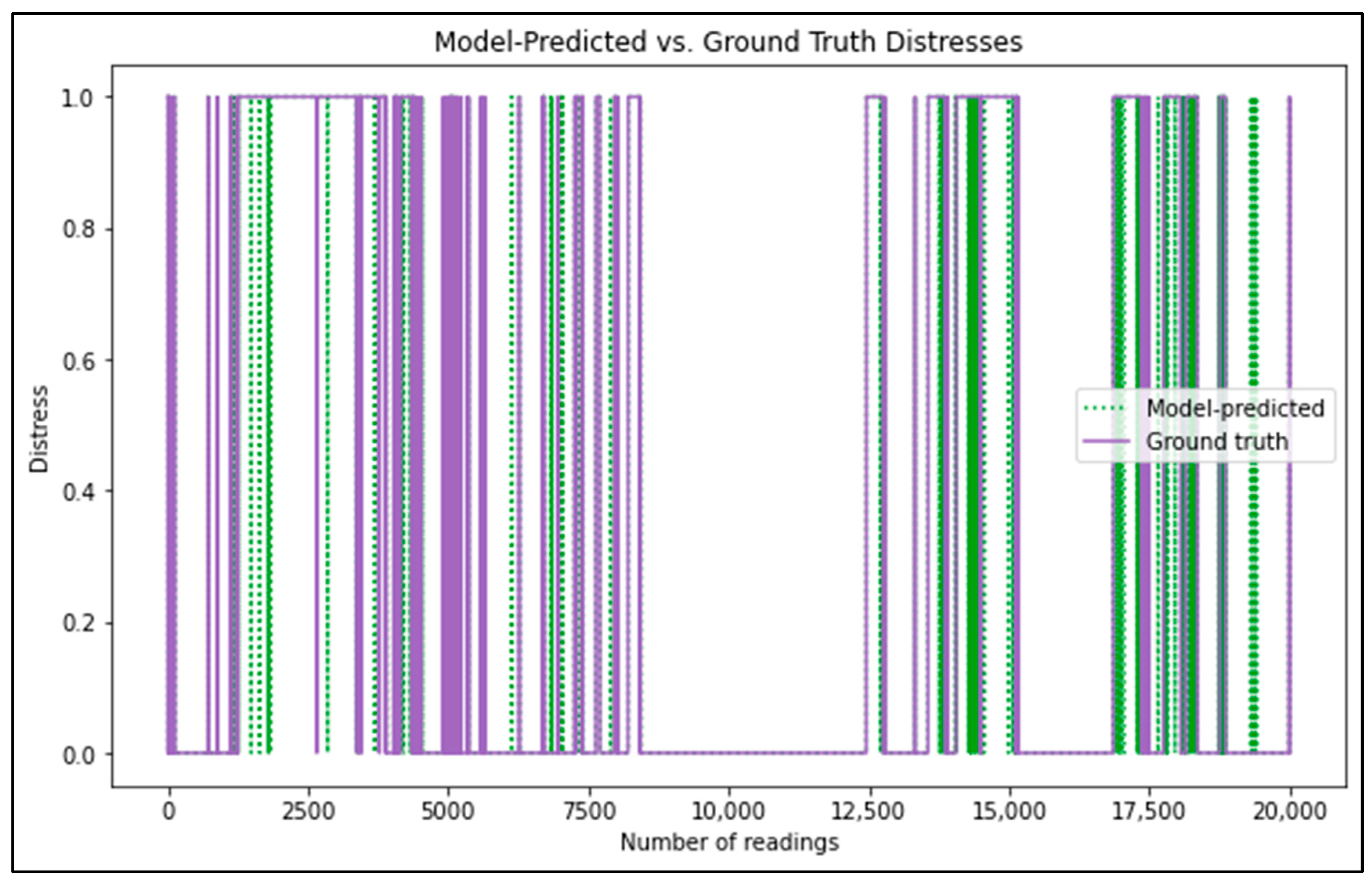
3.5.2. Results of Sensor-based Road Surface Detection Model
3.6. Score the Test Data
4. Conclusions
Limitations and Recommendations of the Study
Author Contributions
Funding
Data Availability Statement
Conflicts of Interest
References
- Ameddah, M.A.; Das, B.; Almhana, J. Cloud-Assisted Real-Time Road Condition Monitoring System for Vehicles. In Proceedings of the IEEE Global Communications Conference (GLOBECOM), Abu Dhabi, United Arab Emirates, 9–13 December 2018. [Google Scholar]
- Engström, R. The Roads’ Role in the Freight Transport System; 6th Transport Research Arena: Göteborg, Sweden, 2016. [Google Scholar]
- Vaitkus, A.; Čygas, D.; Motiejūnas, A.; Pakalnis, A.; Miškinis, D. Improvement of road pavement maintenance models and technologies. Balt. J. Road Bridg. Eng. 2016, 11, 242–249. [Google Scholar] [CrossRef]
- Sahin, H.; Narciso, P.; Hariharan, N. Developing a Five-year Maintenance and Rehabilitation (M&R) Plan for HMA and Concrete Pavement Networks. APCBEE Procedia 2014, 9, 230–234. [Google Scholar]
- Feldman, D.R.; Pyle, T.; Lee, J. Automated Pavement Condition Survey Manual; California Department of Transportation: Los Angeles, CA, USA, 2015.
- USDOT. Distress Identification Manual for the Long-Term Pavement Performance Program; USDOT, Federal Highway Administration: Washington, DC, USA, 2014.
- Ranyal, E.; Sadhu, A.; Jain, K. Road Condition Monitoring Using Smart Sensing and Artificial Intelligence: A Review. Sensors 2022, 22, 3044. [Google Scholar] [CrossRef] [PubMed]
- Majidifard, H.; Jin, P.; Adu-Gyamfi, Y.; Buttlar, W.G. Pavement Image Datasets: A New Benchmark Dataset to Classify and Densify Pavement Distresses. In Proceedings of the TRB 99th Annual Meeting, Washington, DC, USA, 12–16 January 2020. [Google Scholar]
- Sholevar, N.; Golroo, A.; Esfahani, S.R. Machine learning techniques for pavement condition evaluation. Autom. Constr. 2022, 136, 104190. [Google Scholar] [CrossRef]
- Wang, K.C.P.; Zhang, A.; Li, J.Q.; Fei, Y.; Chen, C.; Li, B. Deep Learning for Asphalt Pavement Cracking Recognition Using Convolutional Neural Network. Airfield Highw. Pavements 2017, 166–177. [Google Scholar] [CrossRef]
- Kim, B.; Cho, S. Automated Vision-Based Detection of Cracks on Concrete Surfaces Using a Deep Learning Technique. Sensors 2018, 18, 3452. [Google Scholar] [CrossRef] [PubMed] [Green Version]
- Zhang, A.; Wang, K.C.P.; Li, B.; Yang, E.; Dai, X.; Peng, Y.; Fei, Y.; Liu, Y.; Li, J.Q.; Chen, C. Automated Pixel-Level Pavement Crack Detection on 3D Asphalt Surfaces Using a Deep-Learning Network. Comput.-Aided Civ. Infrastruct. Eng. 2017, 32, 805–819. [Google Scholar] [CrossRef]
- Zhang, A.; Wang, K.C.P.; Fei, Y.; Liu, Y.; Chen, C.; Yang, G.; Li, J.Q.; Yang, E.; Qiu, S. Automated Pixel-Level Pavement Crack Detection on 3D Asphalt Surfaces with a Recurrent Neural Network. Comput. Civ. Infrastruct. Eng. 2019, 34, 213–229. [Google Scholar] [CrossRef]
- Maeda, H.; Sekimoto, Y.; Seto, T.; Kashiyama, T.; Omata, H. Road Damage Detection and Classification Using Deep Neural Networks with Smartphone Images. Comput. Civ. Infrastruct. Eng. 2018, 33, 1127–1141. [Google Scholar] [CrossRef] [Green Version]
- Maeda, H.; Kashiyama, T.; Sekimoto, Y.; Seto, T.; Omata, H. Generative adversarial network for road damage detection. Comput.-Aided Civ. Infrastruct. Eng. 2020, 36, 47–60. [Google Scholar] [CrossRef]
- Aleadelat, W.; Saha, P.; Ksaibati, K. Development of serviceability prediction model for county paved roads. Int. J. Pavement Eng. 2018, 19, 526–533. [Google Scholar] [CrossRef]
- Souza, V.M. Asphalt pavement classification using smartphone accelerometer and Complexity Invariant Distance. Eng. Appl. Artif. Intell. 2018, 74, 198–211. [Google Scholar] [CrossRef]
- Christodoulou, S.E.; Kyriakou, C.; Hadjidemetriou, G. Pavement Patch Defects Detection and Classification Using Smartphones, Vibration Signals and Video Images. Adv. Comput. Strateg. Eng. 2019, 365–380. [Google Scholar] [CrossRef]
- Sandamal, R.M.K.; Pasindu, H.R. Applicability of smartphone-based roughness data for rural road pavement condition evaluation. Int. J. Pavement Eng. 2022, 23, 663–672. [Google Scholar] [CrossRef]
- Pomoni, M. Exploring Smart Tires as a Tool to Assist Safe Driving and Monitor Tire–Road Friction. Vehicles 2022, 4, 744–765. [Google Scholar] [CrossRef]
- Ahmed, N.S.; Huynh, N.; Gassman, S.; Mullen, R.; Pierce, C.; Chen, Y. Predicting Pavement Structural Condition Using Machine Learning Methods. Sustainability 2022, 14, 8627. [Google Scholar] [CrossRef]
- Lekshmipathy, J.; Samuel, N.M.; Velayudhan, S. Vibration vs. vision: Best approach for automated pavement distress detection. Int. J. Pavement Res. Technol. 2022, 13, 402–410. [Google Scholar] [CrossRef]
- Eisenbach, M.; Stricker, R.; Seichter, D.; Amende, K. How to get pavement distress detection ready for deep learning? A systematic approach. In Proceedings of the 2017 International Joint Conference on Neural Networks (IJCNN), Anchorage, AK, USA, 14–19 May 2017; pp. 2039–2047. [Google Scholar]
- Hamishebahar, Y.; Guan, H.; So, S.; Jo, J. A Comprehensive Review of Deep Learning-Based Crack Detection Approaches. Appl. Sci. 2022, 12, 1374. [Google Scholar] [CrossRef]
- Gur-Arie, P.L. The Practical Guide for Object Detection with YOLOv5 Algorithm. 14 January 2023. [Online]. Available online: https://towardsdatascience.com/the-practical-guide-for-object-detection-with-yolov5-algorithm-74c04aac4843 (accessed on 12 November 2022).
- Ramanishka, V.; Chen, Y.-T.; Misu, T.; Saenko, K. Toward Driving Scene Understanding: A Dataset for Learning Driver Behavior and Causal Reasoning. In Proceedings of the IEEE Conference on Computer Vision and Pattern Recognition (CVPR), Salt Lake City, UT, USA, 18–22 June 2018; pp. 7699–7707. [Google Scholar] [CrossRef]
- Garg, A. How to Use Yolo v5 Object Detection Algorithm for Custom Object Detection. Available online: https://www.analyticsvidhya.com/blog/2021/12/how-to-use-yolo-v5-object-detection-algorithm-for-custom-object-detection-an-example-use-case/ (accessed on 6 January 2023).
- Justo-Silva, R.; Ferreira, A.; Flintsch, G. Review on Machine Learning Techniques for Developing Pavement Performance Prediction Models. Sustainability 2021, 13, 5248. [Google Scholar] [CrossRef]
- XGBoost. XGBoost Parameters. XGBoost Developers. Available online: https://xgboost.readthedocs.io/en/stable/parameter.html (accessed on 26 February 2023).
- Allwright, S. What Is a Good F1 Score and How Do I Interpret It? Available online: https://stephenallwright.com/good-f1-score/ (accessed on 28 July 2022).
- Montgomery, D.C.; Runger, G.C. Applied Statistics and Probability for Engineers; Wiley: Hoboken, NJ, USA, 2018. [Google Scholar]
- Mcdowell, I. Measuring Health: A Guide to Rating Scales and Questionnaires; Oxford University Press: Oxford, UK, 2006. [Google Scholar]
- Chen, T.; Guestrin, C.E. XGBoost: A Scalable Tree Boosting System. In Proceedings of the 22nd ACM SIGKDD International Conference on Knowledge Discovery and Data Mining, San Francisco, CA, USA, 13–17 August 2016. [Google Scholar]


| S/N | Parameter | Value |
|---|---|---|
| 1 | Batch Size | 40 |
| 2 | Epochs | 150 |
| 3 | Learning Rate | 0.01 |
| 4 | Optimizer | SGD = 1 × 10⁻² |
| 5 | Anchor Sizes | Dynamic |
| S/N | Parameter | Value |
|---|---|---|
| (a) | ||
| 1 | learning rate | 0.1 |
| 2 | max depth | 3 |
| 3 | n_estimators | 5000 |
| 4 | subsample | 0.5 |
| 5 | colsample_bytree | 0.5 |
| (b) | ||
| 1 | learning_rate_list | [0.02, 0.05, 0.1] |
| 2 | max_depth_list | [2, 3, 5] |
| 3 | n_estimators_list | [1000, 2000, 3000] |
Disclaimer/Publisher’s Note: The statements, opinions and data contained in all publications are solely those of the individual author(s) and contributor(s) and not of MDPI and/or the editor(s). MDPI and/or the editor(s) disclaim responsibility for any injury to people or property resulting from any ideas, methods, instructions or products referred to in the content. |
© 2023 by the authors. Licensee MDPI, Basel, Switzerland. This article is an open access article distributed under the terms and conditions of the Creative Commons Attribution (CC BY) license (https://creativecommons.org/licenses/by/4.0/).
Share and Cite
Ruseruka, C.; Mwakalonge, J.; Comert, G.; Siuhi, S.; Ngeni, F.; Major, K. Pavement Distress Identification Based on Computer Vision and Controller Area Network (CAN) Sensor Models. Sustainability 2023, 15, 6438. https://doi.org/10.3390/su15086438
Ruseruka C, Mwakalonge J, Comert G, Siuhi S, Ngeni F, Major K. Pavement Distress Identification Based on Computer Vision and Controller Area Network (CAN) Sensor Models. Sustainability. 2023; 15(8):6438. https://doi.org/10.3390/su15086438
Chicago/Turabian StyleRuseruka, Cuthbert, Judith Mwakalonge, Gurcan Comert, Saidi Siuhi, Frank Ngeni, and Kristin Major. 2023. "Pavement Distress Identification Based on Computer Vision and Controller Area Network (CAN) Sensor Models" Sustainability 15, no. 8: 6438. https://doi.org/10.3390/su15086438