A New Framework of 17 Hydrological Ecosystem Services (HESS17) for Supporting River Basin Planning and Environmental Monitoring

Abstract

Hydrological ecosystem services (HESS) describe the benefits of water for multiple purposes with an emphasis on environmental values. The value of HESS is often not realized because primary benefits (e.g., food production, water withdrawals) get the most attention. Secondary benefits such as water storage, purification or midday temperature cooling are often overlooked. This results in an incorrect evaluation of beneficial water usage in urban and rural resettlements and misunderstandings when land use changes are introduced. The objective of this paper is to propose a standard list of 17 HESS indicators that are in line with the policy and philosophy of the Consultative Group of International Agricultural Research (CGIAR) and that are measurable with earth observation technologies in conjunction with GIS and hydrological models. The HESS17 framework considered indicators that can be directly related to water flows, water fluxes and water stocks; they have a natural characteristic with minimal anthropogenic influence and must be quantifiable by means of earth observation models in combination with GIS and hydrological models. The introduction of a HESS framework is less meaningful without proper quantification procedures in place. Because of the widely diverging management options, the role of water should be categorized as (i) consumptive use (i.e., evapotranspiration and dry matter production) and (ii) non-consumptive use (stream flow, recharge, water storage). Governments and responsible agencies for integrated water management should recognize the need to include HESS17 in water allocation policies, water foot-printing, water accounting, transboundary water management, food security purposes and spatial land-use planning processes. The proposed HESS17 framework and associated methods can be used to evaluate land, soil and water conservation programs. This paper presents a framework that is non-exhaustive but can be realistically computed and applicable across spatial scales.

1. Introduction

Ecosystem services are defined as the goods and services provided by ecosystems that are direct and indirect contributions to human well-being [1,2]. Ecosystem services are the benefits that people and societies receive from nature, such as food, water, pollination, nutrient cycling and many others. Hydrological ecosystem services (HESS), also referred to as water-related ecosystem services, link these services to the hydrological cycle, thus making explicit that the magnitude of the ecosystem service depends on water availability, i.e., quantity and quality. For example, certain stream flow regimes are required for maintaining fish, birds and perennial corridors that provide food and income for local people [3]. Recurring rainfall is required for keeping dryland agro-forestry ecosystems productive. The hydrological processes of the unsaturated zone control gaseous exchanges in water vapor (H₂O), carbon dioxide (CO₂), methane (CH₄), ammonification (NH₄) and nitrous oxide (N₂O) between land and atmosphere, thereby regulating atmospheric greenhouse gas concentrations and warming of the earth. Vegetated surfaces have great ecological value, but they require certain soil moisture regimes for sufficient photosynthesis. The World Wide Assessment Program (2018) [4] synthesized the international developments on nature-based solutions (NbS) for water and highlighted the growing emphasis on the inclusion of ecosystem services as quantifiable benefits into integrated land and water resource management around the world. The Consultative Group of International Agricultural Research (CGIAR) established its Ecosystem Services and Resilience Framework (ESR) defining an ecosystem service-based approach to build community resilience and restore ecosystem services for provisioning goals or in ways that support and regulate these goals, while reducing the negative impacts on the natural resource base that underpins these ecosystem services [5]. CGIAR’s ESR provided an excellent entry point for creating a minimal list of HESS indices that followed ES characteristics and quantification methods, i.e., use of earth observation data in combination with GIS and eco-hydrological tools. The use of scenarios and models for HESS quantification allows a pragmatic approach to support decision making in river basin planning and environmental monitoring within time and space boundaries [6]. Examples include assessment of marginal benefits to nature and humans as consequences from basin management alternatives. Furthermore, inclusion of HESS ensures the transition from traditional top-down and single objective systems into multi-criteria and human-centred approaches that can prioritize activities with a broader spectrum of benefits [7]. Especially, HESS ensures the uptake of international guidance, such as integrated water resources management (IWRM), by achieving a win-win co-development of water with, among others, land and ecosystems, while fully delivering the benefits to humans and society [8].

The quantification of HESS has become one of the fastest growing areas of environmental research [9]. Yet, due to the absence of operational information systems, policy makers continue with business as usual. Clear definitions and explanatory methods for quantification of HESS are vital to close this policy–practice gap. Both the benefits and the water volumes needed to establish these benefits must be estimated across areas with spatially variable physiographic conditions.

The lack of a standardized framework and consensus for quantifying HESS as a spatial process limits the uptake by policy makers and managers [10,11,12]. In this context, the development of a minimum list of HESS indicators is a great contribution to ecosystem services research. Such a framework would improve comparability between river basins and watersheds and help people understand the impacts of longer term policies, implementation plans, projects and investments on achieving a healthier water-related ecosystem.

Analytical tools for spatial assessment of HESS have been developed [7,10] including distributed hydrological models, e.g., soil and water assessment tool (SWAT) [13,14]; ecosystem services-oriented tools, e.g., integrated tool to value ecosystem services (InVEST) [15]; or artificial intelligence for ecosystem services (ARIES) [16]. SWAT has the ability to connect surface water, soil moisture and groundwater hydrologically using local land use and soil information to further water quality and food production [11,17]. Various elements of HESS such as water yield, water purification and sediment retention can be assessed by tools such as InVEST [18,19]. A different form of HESS modelling was outlined by Simons et al. [20] who demonstrated how publicly available earth observation data sets can be applied to generate HESS assessments at pixel level. Using pixels of 250 m × 250 m or 1 km × 1 km provides new opportunities to locally report HESS.

The objective of the current paper is to describe a framework for HESS indicators which is in line with the policy and philosophy of CGIAR [5]. Seventeen HESS indicators will be proposed and possible methodologies to quantify them will be discussed using remote sensing, GIS and hydrological models. This list is not exhaustive and can always be expanded; it should be considered as a first attempt in the direction of standardization. An accompanying paper [21] shows a practical example of HESS determination in the Red River, Vietnam.

2. Brief Literature Review of Hydrological Ecosystem Services (HESS)

The Consultative Group on International Agricultural Research (CGIAR) on Water, Land and Ecosystems published a comprehensive report on ecosystem services and a resilience framework [5]. Similar to TEEB (2010) [22], ESR catalysed the flow of ecosystem services to and from agriculture to increase production and subsequently food and livelihood security. In terms of a HESS framework, Grizzetti et al. [11] developed an analysis framework for inland waters in European basins considering the links between pressures, ecological status and ecosystem services. In this study, four HESS attributes were identified, i.e., water quantity (including seasonality), water quality, biological quality elements and hydromorphological/physical structure. Focusing on the way ecosystems affect hydrologic attributes, i.e., water quantity, quality, location of delivery and timing of delivery, Brauman et al. [23] presented a framework for defining and assessing HESS attributes, which translate eco-hydrological processes into an ecosystem service context useful to decision makers; it included water for municipal use, hydropower, recreation, fish supply, reduction in flood damage, water and nutrients to support vital estuaries and other habitats, preservation of options, etc. With a similar end result, Belmar et al. [24] assessed the relationships between annual mean discharges, fish populations and shellfish species (prawns and shrimps) in the lower Ebro. The mean annual discharge was able to explain the variation in fish-based ecological quality; model performance increased when aquatic vegetation was incorporated. Among HESS studies focusing on provisioning and regulation, Poff et al. [25] introduced the ELOHA framework which considers a number of hydrological and ecological processes for different river types to understand the linkages between hydrologic, ecological and social aspects of environmental flow assessment. These relationships are established based on paired streamflow and ecological data from throughout the region of interest. Similarly, Pan and Choi [26] developed a conceptual framework for HESS consisting of a temporal demonstration of water provision, flood control and sediment regulation in the Milwaukee River Basin (US) based on ground observation of streamflow and sedimentation for calibration.

In terms of HESS quantification and trade-off analyses, Gao et al. [27] analysed land-use change and corresponding variations in water-related ecosystem services, i.e., water yield, soil conservation and water purification services in the Guishui River Basin, China. Their study underscored that HESS services were greatly affected by different land-use change scenarios. Thus, land-use and water-use policies should include water-related ecosystem services. Willaarts et al. [28] empirically assessed the relationship between the use and management of agroecosystems, their hydrological functioning and HESS, through a list of nine HESS indicators including forage, drinking water, flow regulation, recreation, olive crops and cork production, meso-climate regulation, hydropower generation and maintenance of aquatic biodiversity. Bangash et al. [29] evaluated the impacts of climate change in the water provisioning and erosion control services in the densely populated Mediterranean Llobregat River Basin (Spain). Their study found that drinking water is expected to decrease between 3 and 49%, while total hydropower production will decrease between 5 and 43%. Fan et al. [30] determined water yield, inorganic nutrients, organic nutrients and sediment retention in the Teshio watershed (Japan) using the SWAT model. The results indicate that HESS provides an effective trade-off between environmental protection (sediment and organic nutrient retention) and economic development (water yield and inorganic nutrient retention).

The point of this brief review is to highlight that authors often have similar thoughts on the usefulness of water resources for the environment, with diverging and often ambiguous definitions; however, quantification methods are not ambiguous. Existing frameworks on interpretations of HESS are comprehensive and contain indicators that are amenable to quantification. The inclusion of supporting and cultural services is often overlooked and questionable in terms of a quantification method [31]; nonetheless, it seems to be necessary for consideration in any framework. Similar discussions on the segregation of supporting services from provisioning and regulating indicate that different views still exist [1,5,32].

For this reason, we aim at defining a minimum and standard list of 17 HESS indicators congruent with the CGIAR framework.

3. Definition of the Hydrological Ecosystem Services (HESS) Framework

3.1. Formulation of the HESS17 Framework

A minimum list of HESS indicators was taken from the CGIAR report using certain criteria. The formulation of this non-exhaustive framework on HESS and their quantifications are underpinned by the view that a conceptualized and standardized assessment skeleton of multiple values of hydrological ecosystems and their benefit to humans needs to be recognized and valued. Through this process, priorities on the development pathways and scenarios that most benefit people while adequately address the challenge of sustainability at different scales, e.g., global, river basin or community level [33]. There are numerous frameworks that establish as a priority the use of models for monitoring of provisioning and regulating services, such as water provisioning or soil erosion [15,18]. However, there is a shortage of approaches that can incorporate values of HESS into river basin management and across the nature–human sphere. This shortcoming occurs in two aspects: the first is providing a conceptualization, seamless valuing and representation of hydrological ecosystem services in provisioning, regulating, supporting and cultural functions; the second is their ability to include the development of scenarios and pathways across scales and benchmark the level of sustainability. Another characteristic of the HESS17 framework is its capability to provide an ample space for adding more indicators in the future, following the implementation of SDGs or achievement of human development targets.

Existing frameworks [1,11,25] show a greater abundance and clear imbalance towards provisioning and regulation services rather than cultural and support services; many studies solely focus on the former [9,29]. This drawback results from the characteristics of HESS in that they have a much stronger connection to regulation and provisioning services, i.e., water flows, storage and moisture circulation, than on cultural and/or habitat services. In this framework, we aim to have a full spectrum of indicators from the entire four HESS categories by including HESS that represent supporting and cultural services. The selected set of HESS indicators succinctly defines how multiple values of ecosystems and their contributions to people should be acknowledged. Selected HESS indicators should fulfil certain criteria: they should be water flows, water fluxes and water stocks; they should also be clearly adhered to a natural function or process of the ecosystem with minimal anthropogenic influence; and they must be quantifiable by means of earth observation models in combination with GIS and hydrological models. Apart from considering HESS properties, the HESS17 aims to catalyse the interactions between eco-hydrological components and processes and build up a feedback mechanism that reflects human–nature relationships, e.g., through the simulation of land use changes, urban heatwave, agricultural production and an investigation of NbS outcomes. The valuation and assessment of feedback functions will allow the calculation of benefits and expenses of HESS in spatially and temporally explicit manners [18]. Examples of this are the generation of runoff or maintenance of dry season flows from upstream, which can benefit downstream communities or the improvement in sustaining rainfall within the basin’s perimeter through effective water management.

The HESS indicators should not be related to specific remote sensing algorithms or numerical models. McCartney et al. [34] emphasized that HESS should be based on natural water services in pristine environments and landscapes; this is a narrower view that emphasizes mainly the role of natural lakes and wetlands as natural sponges that retain water and reduce peak flows. While this is fundamental, a broader view of natural benefits from water consumption is necessary. Natural vegetation communities consume vast amounts of water, and their benefits for living organisms are significant, ranging from the provision of shade to biodiversity, to insects that enhance pollination. The consumptive use of water resources in river basins, e.g., evapotranspiration, forms the basis for various environmental services, such as sustaining rainfall or providing micro-climate cooling. It is a key process since these water resources originated from surface water and groundwater flows and stocks; thus, they should be utilized as responsibly as possible [35,36,37,38,39]. The general categories of ecosystem descriptions are fresh water, food, fuels, fresh water supply, disturbance regulation, air climate and quality, water quality, habitat provision and recreation (see

Table 1. Proposed framework of 17 hydrological ecosystem services (HESS) based on a CGIAR workshop.

General Categories	HESS	Ecosystem Services/Concept	Major Principles	Unit	Spatial Connection between Providing and Demanding Locations of HESS	Temporal Connection between Providing and Demanding Locations of HESS	Consumptive Use	Non-Consumptive Use
		Provisioning services (related to water)
Fresh water	1	Basin runoff	Ultimate source of water available for multiple purposes	m3/ha	River basin, in-stream directional benefits (downstream)	Annual, seasonal (wet and dry period)		x
Food	2	Inland capture fishery	Catch from lakes, wetlands, rivers	kg/ha	Local, surrounding communities	Annual	x	x
Food	3	Natural livestock feed production	Dry matter production from natural pastures, alpine pastures, wetlands and more	kg/ha	Local, surrounding communities	Annual	x
Fuels	4	Fuelwood from natural forests	Dry matter production from forests and savannahs	kg/ha	Local, surrounding communities	Annual	x
		Regulating services (related to water)
Fresh water supply	5	Dry season flow (“baseflow”)	Flow from groundwater outflow, lakes, wetlands and upstream runoff	m3/s	River basin, directional benefits (downstream)	Seasonal (during dry period)		x
Fresh water supply	6	Total groundwater recharge	Vertical transient moisture flow originating from percolation reaching saturated groundwater	m3/ha	River basin	Annual, seasonal (wet and dry period)		x
Fresh water	7	Surface water storage	Total water stock in natural surface water systems (lakes, wetlands)	m3	River basin, local, surrounding communities	Annual, seasonal (wet and dry period)		x
Fresh water supply	8	Root zone water storage	Retention of soil moisture in unsaturated zone for carrying over water from wet to dry seasons	m3	River basin, local, surrounding communities	Annual, seasonal (wet and dry period)		x
Fresh water supply	9	Sustaining rainfall	Sustaining rainfall originating from land evaporation	m3/ha	River basin	Annual	x
Disturbance regulation	10	Peak flow attenuation	Attenuated peak flow for safeguarding downstream areas from flooding by means of ecological intervention	%	River basin, directional benefits (downstream)	Seasonal (wet period)		x
Air quality and climate	11	Carbon sequestration	Assimilating atmospheric carbon into crop organs (wood, roots) and soil	kg C/ha	River basin	Annual	x
Air quality and climate	12	Reduce greenhouse gas emissions	Reduced methane emissions and other trace gasses due to changes in land use and water management	kg C/ha	River basin	Annual	x
Air quality and climate	13	Micro-climate cooling	Evaporative cooling of the vegetation and near-surface atmosphere due to changes in land and water management	°C	River basin	Annual	x
Water quality	14	Natural reduction of water eutrophication	Reduction in eutrophication due to changes in land use and water management	%	River basin, directional benefits (downstream)	Annual, seasonal (wet and dry period)		x
Water quality	15	Reduction in soil erosion	Reducing erosion and sedimentation by increased vegetation cover	kg/ha	River basin, directional benefits (downstream)	Annual, seasonal (wet and dry period)	x
		Supporting services
Habitat provision	16	Meeting environmental flow requirements	Meeting minimum flows and water levels for biodiversity, ecosystem health and endangered (fish) species	%	River basin, in-stream directional benefits (downstream)	Seasonal (wet and dry period)		x
		Cultural services
Recreational	17	Leisure	Socialisation of humans via water sports, golf courses, eco-tourism, aesthetic views, mountain biking, forest BBQs, etc.	Number of visitors	Local, surrounding communities	Annual, seasonal (wet and dry period)	x	x

). They can be synthesized into provisioning, regulating, supporting and cultural services. Because of the irreversible character of consumptive use, it is sound to separate HESS into processes that are related to consumptive use (e.g., evapotranspiration) and non-consumptive use (e.g., runoff, percolation, baseflow). Furthermore, one remaining question in addressing HESS is the spatial–temporal connection between locations that are providing and demanding HESS, i.e., where are HESS produced and where are HESS consumed? The proposed HESS framework aims to delineate these spatial–temporal relations by identifying the locations that are providing and those that are demanding, i.e., at the larger river basin scale or in localities where HESS is consumed by local communities, and the time aspect of when benefits or potential demands for HESS can be mapped.

In total, 17 HESS were identified and selected, categorized into provisioning (4), regulating (11), supporting (1) and cultural (1) services.

3.2. Definition of HESS Presented in the Framework

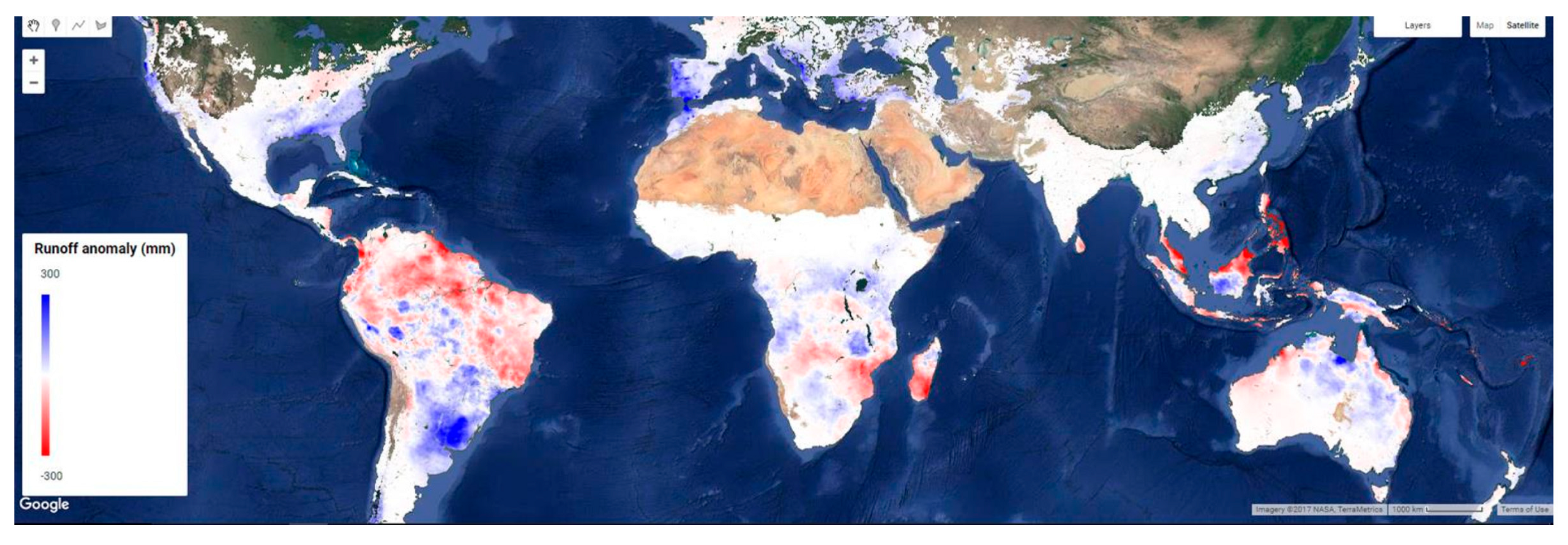
3.2.1. HESS1: Basin Runoff

Basin runoff (HESS1) from a river basin is the amount of surface and groundwater resources that are generated internally in a watershed or river basin. Inflows from upstream basins is excluded. Surface runoff creates stream and river flows which are the source for aquatic ecosystems. Excess water from the surface network and the unsaturated soil through leakage and percolations feeds aquifer systems that convey water laterally and interact with streams. Because surface water can become groundwater and vice versa, the term basin runoff is preferred for defining HESS1.

At the aggregate level of the basin, basin runoff is the sum of surface runoff into streams and natural percolation from the root zone into drainage networks and aquifers (this excludes non-natural percolation arising from water resource withdrawals). The baseflow is ultimately available in streams as flows during the dry season. Interflow occurs on undulating or sloping terrain where unsaturated zone moisture has a lateral component due to layered soil properties, perched water tables, etc. Because HESS1 represents the basin runoff, the exact flow path of water to reach streams and rivers, as well as the stream flow, are less relevant.

Basin runoff is the primary source for all multi-purpose withdrawals, both naturally (e.g., floods, lakes, groundwater dependent ecosystems) and manmade withdrawals (e.g., domestic, industry, irrigation). Natural withdrawals can be significant, and blue water resource consumption related to withdrawals is not available for other usage [23,38,40].

A simple t definition of basin runoff is precipitation minus ET from green water resources (P-ETgreen), sometimes indicated as net precipitation. This definition excludes all water withdrawals (including natural withdrawals). Water stored in permanent surface and groundwater systems should also be subtracted from basin runoff.

Several papers have been published that show how P can be solved from earth observations, e.g., [41,42]. Different energy balance models can be chosen for the estimation of ET, e.g., [43,44]. Spatial ET data can also be used for various types of hydrological analysis, e.g., [14]. The GRACE gravity mission measures the changes in water storage $\mathsf{\Delta }\mathrm{S}$ in an independent manner [45,46]. P, ET and ∆S together can be used to assess basin runoff.

3.2.2. HESS2: Inland Capture Fishery

HESS2 describes the fish catch from inland lakes, rivers, mangroves, lagoons and other natural water bodies. The catch from these waters is of economic value and provides nutrients to local communities. Specific flow regimes are an asset for prawning, fish migration and fish catch. Most freshwater fish have evolved life cycles that are adapted to natural river habitat and flow regimes. The evaporation from these water systems can be considered as the water consumed for achieving the fish catch. Information on the size of open water bodies together with the evaporation from water bodies is required to relate inland capture fisheries to water consumption.

Information on the capture of inland fish can come from standardized statistical records. The database of FAOSTAT [47] and WorldFish [48] are good options to obtain data and they reveal a linear growth over the last 50 years. FAO estimates that 12 million tonnes of inland fish were captured in 2018; this was 6.7% of total fish production [49]. Marine capture is seven times more than inland capture. Current data are sufficient only for a general overview of global inland catches of fish, rather than for the detailed analysis needed for management, policy formulation and valuation of inland fisheries [50].

Several studies [51,52,53] illustrated the use of different spectral indicators to identify the size of water bodies using optical data. During monsoon with frequent cloud cover and floods, the quality of the optical data is hampered, and it is customary to use synthetical active radar (SAR) data. Rebelo et al. [54] and Donlon et al. [55] showed how Sentinel-3 SAR data can be best utilized. Various techniques consisting of L-band synthetic aperture radar (SAR) [56], Landsat and SPOT [57] were used to monitor the status of and changes in wetlands, both rainfed and water bodies, to calculate fisheries’ yield based on a yield-per-unit area approach. The combination of size of the open water area, water level and water evaporation was sufficient to compute the consumptive use of water bodies on a volume basis.

3.2.3. HESS3: Natural Feed for Livestock

HESS3 deals with the natural feed for livestock owned by pastoralists and wild livestock such as mountain sheep, wild mammals, cats, elephants and the like. Cattle and cats graze on several types of natural pastures (grass fields, savannah, steppes, alpine, wetlands). Their feed is a result of photosynthesis and water consumption (ET). HESS3 is essential for many national parks and extensive savannah landscapes.

The physical processes of dry matter production of grasslands are widely studied. Various versions of net primary production (NPP) models exist for the computation of the net carbon flux of pastureland. While NPP models are often made for global ecological studies, they can also be applied on a pixel by pixel basis. Hence satellite measurements can be used to determine NPP and dry matter production. Remotely sensed data from multispectral satellites, e.g., MODIS, Landsat, Sentinel-2, etc., can be used to assess grassland’s greenness and thickness while optical sensors can capture biophysical and biochemical information [58]. Monteith’s model [59] for the production of pasture is based on absorbed photosynthetically active radiation (APAR) and a light use efficiency (LUE) conversion factor. LUE values for grassland vary typically between 1.6 to 2.8 gr/MJ, depending on soil moisture, temperature, vapor pressure deficit and grass nitrogen status [60].

A first distribution of the crop organs is between above- and below-ground accumulated dry matter production. This is classically expressed by means of the root/shoot ratio, which is 1.5 to 2.5 for grassland. Hence, above-ground production is approximately 33% of the accumulated total dry matter production. Furthermore, not all above ground dry matter production can be considered livestock feed. An amount of 25% of the accumulated dry matter production of cropland is assumed to be available for feed. In addition, residues from field crops (e.g., stems and leaves not taken away during the harvest process) are also part of the natural feed. Part of the dry matter production from these specific land use classes related to pasture and crop residues should therefore be HESS3 inclusive.

3.2.4. HESS4: Fuelwood

Fuelwood includes firewood, charcoal, chips, sheets, pellets and sawdust. Fuelwood is used for cooking and heating in developing countries, where it is of great value for the livelihoods of local communities. Fuelwood is a co-product of forestry, timber production and woodland management. HESS4 addresses fuelwood from natural forests and savannahs, but not from plantations. Roughly 25% of global fuelwood is produced in sub-Saharan Africa. One ton of charcoal requires five tons of wood [61]. Similar to HESS3, fuelwood can be computed from NPP models or earth observations of APAR and LUE [62].

The ratio of above to total dry matter production of woody vegetation types is typically 60 to 80%. Trischler et al. [63] found that above-ground carbon assimilates are 65% of the total production value for common tree species in Sweden. In Ethiopia, Pukkala and Pohjonen [64] showed fresh wood production for eucalypt in a range from 7 to 35 ton/ha/yr. Fresh wood production of 20 ton/ha/yr is approximately 14 ton/ha/yr dry wood. Several remote sensing algorithms are also available for the assessment of ET in forests, e.g., [65,66].

3.2.5. HESS5: Dry Season Flow

Dry season flow—HESS5 (also called base flow, drought flow, groundwater recession flow)—is the portion of the streamflow that originates from the lateral groundwater flow that seeps into the river channel. The stream flow during the dry season is fundamental for humans disconnected from water utilities, livestock and environmental systems that only survive due to daily access to water resources. Pollutants need to be diluted and evacuated towards seas and oceans, and HESS5 also contributes to that process. HESS5 is a regulating service.

The recession limb of the hydrograph reveals the point where the river’s level falls to a level where baseflow becomes the major source of stream flow. The hydrograph is obtained typically from hydrological models, although there is more literature on the assessment of flow from earth observations. Yang et al. [67] and Donchyts et al. [68] showed that river widths can be delineated using multi-scale classification approaches. The width of rivers containing water is essential for assessing whether baseflow is occurring. If the water body area dried up, it can be concluded that the base flow has vanished. Bjerklie et al. [69] demonstrated an integrated methodology to assess discharge, flow depth, and flow velocity determined from remotely observed water surface area, water surface slope, and water surface height for two reaches of the Yukon river. Durand et al. [70] described the determination of river height, river width and river slope. Michailovsky and Bauer-Gottwein [71] showed the development of a generic 1D stream flow Manning equation to assess river discharges based on these river dimensions. The surface water and ocean topography (SWOT) satellite mission planned for launch in 2022 will map river elevations and inundated areas globally for rivers > 100 m wide. Figure 1 illustrates an application of Sentinel-3A altimeter data for detecting water level change in river [72].

3.2.6. HESS6: Total Groundwater Recharge

Aquifers are often considered the “bank savings accounts” to abide periods of drought. Groundwater recharge from rainfall describes the renewable groundwater resources and HESS6 forms the source of multi-sector groundwater abstractions and baseflows to feed streams during periods without surface runoff. It is the source for total water storage underground where there are no evaporation losses. HESS6 is fundamental for preparing long term groundwater allocation plans to ensure sustainable withdrawals for several users. While HESS1 focuses more on natural recharge processes, HESS6 relates to the total recharge from various sources to maintain water in underground stocks for periods when it is needed the most.

While water from leaking irrigation fields, reservoirs and artificially created canals is clearly an example of anthropogenic recharge $q_{anth}^{\downarrow }$ [73], it is believed nevertheless to be valuable for describing total recharge as an ecosystem service, for instance to ensure sufficient drinking water for the domestic sector. Recharge from a leaking river $q_{riv}^{\downarrow }$ is partially natural, but also partially anthropogenic because river flow is a result of upstream interventions in the water cycle. These can be the building of dams and reservoirs, but also diversions of surface water and the changes in land use that accelerate flow after heavy rainfall events.

Percolation occurs when soil moisture of the unsaturated zone exceeds its field capacity and drainable flow limits. Thus, wet soils and water bodies contribute significantly to recharge and more than, for instance, settlements and rainfed cropland that usually have a soil moisture content that is lower than field capacity. The most widely accepted mathematical solution for computing percolation fluxes in the unsaturated zone is Richard’s equation for vertical and transient soil moisture flow; it is a combination of Darcy’s law for water flux in unsaturated soils and the continuity equation. However, local knowledge on these soil hydraulic properties are not common, and numerical models for solving Richard’s equation are difficult to operate [8]. Alternative solutions have been worked out, such as the chloride mass balance (CMB), rainfall infiltration breakthrough (RIB), extended model for aquifer recharge and moisture transport through unsaturated hard rock (EARTH), water table fluctuation (WTF), water balance in the saturated zone (including equal volume spring flow (EVSF) and saturated volume fluctuation (SVF)) and groundwater modelling (GM) (see Xu and Beekman [74] for a review of these processes). Wohling et al. [75] elaborately summarize various methods for Australia, including the role of rainfall, clay content, vegetation basal area, leaf area index, depth to water table and hydraulic conductivity on estimating recharge in a practical manner. Hessels et al. [76] introduced an elegant method to compute percolation fluxes from the root zone on the basis of soil water balance residuals of green water pixels.

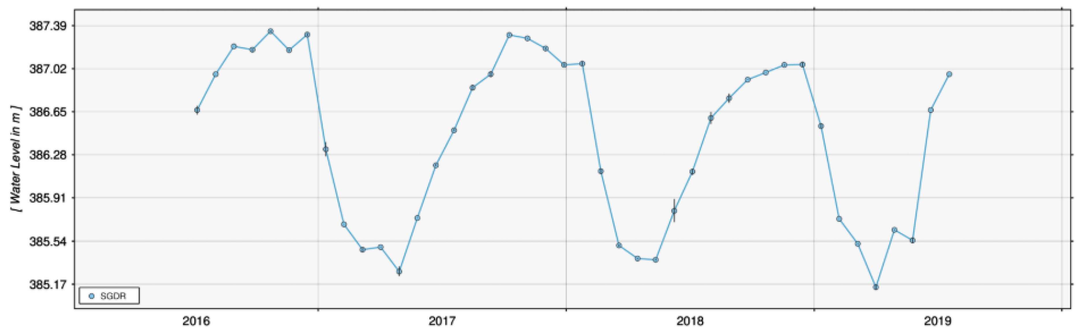
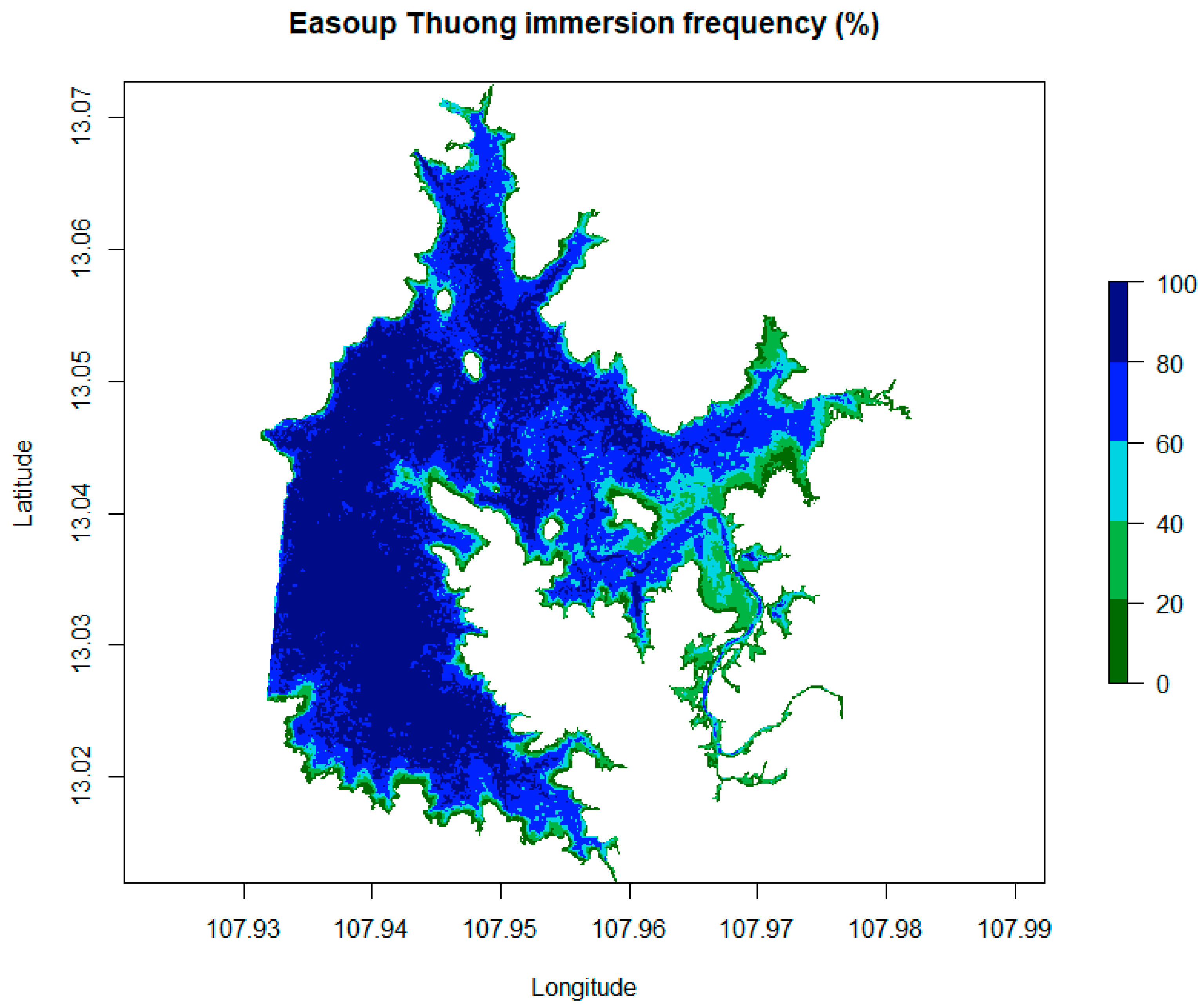
3.2.7. HESS7: Surface Water Storage

HESS7 describes water stocks, excluding rivers and reservoirs. It is the amount of blue water present in natural surface water systems (lakes, wetlands, lagoons). Rivers provide little storage at a monthly scale and is therefore negligible. Trends in natural water storage are meaningful information for the health of hydrological ecosystems and for the retention of water to carry over resources during drier spells. Water storage in lakes and wetlands enhances ecosystem services because it is indistinguishably linked to various services, such as water retention during floods and attenuation of peak flow; water supply during elongated droughts; water for agriculture (cropping systems on banks; livestock water supply, fish); water-related habitats for migratory birds and water-related mammals; cooling off hot air masses; and leisure opportunities.

Rebelo et al. [54] conducted an overview of wetland distribution, type and condition across sub-Saharan Africa and showed that local communities highly rely on both wetland agriculture and natural resources. The areal size of open water bodies in lakes, wetlands, lagoons and mangroves can be computed from satellite measurements [77] (see also Figure 2). Water depth can be estimated from water level fluctuations using satellite-based altimetry which, in combination with area, can be used to assess surface water stocks [78].

3.2.8. HESS8: Root Zone Water Storage

The root zone has an important regulating role in infiltration, retention, storage and root water uptake for the transpiration of local vegetation systems. The root zone connects geology, pedology and biology. The soil water retention characteristic, in conjunction with root depth, dictates the amount of water that can be retained in the sub-surface. The soil water-holding capacity is the difference between soil moisture at field capacity and at wilting point [79]. It varies typically between 50 to 250 mm/m. Deeper root systems (e.g., more than 1 m) can store vast quantities of water (>5000 m³/ha) and carry water over from the rainy season to the dry season, even from wet winters to dry winters. Root zone water is the first and utmost important supplier of water for vegetation in the dry season [80]. Hence, HESS8 expresses the capture of soil water during periods with a positive rainfall surplus. Because land surface containing roots is significantly larger than open water bodies, HESS8 is a crucial regulator of climatological deficits and excess water.

Most remote sensing techniques for the determination of soil moisture are based on radar and microwave technologies, e.g., [81,82]. This technique is at best useful for detecting skin moisture under sparse vegetation. Microwave vegetation optical depth (VOD) describes the attenuation of radiation due to scattering and absorption within the vegetation layer, which is caused by the water contained in the vegetation [83]. The optical depth of the vegetation is a serious constraint for measuring skin soil moisture [84].

Moisture in the root zone can therefore be best inferred from the land surface temperature of vegetated surfaces. The temperature of the vegetation reflects sub-soil processes such as root development, storage capacity of the soil and soil water potential. Various remote sensing solutions are therefore based on inferring soil moisture in the root zone from evapotranspiration processes, e.g., [85,86,87] or from soil thermal inertia [88]. Carlson and Petropoulos [89] and Yang et al. [90], among many others, used the trapezoid between land surface temperature and vegetation index to infer a relative value for soil moisture. These techniques are much simpler than microwave measurements and appeared successful in operational and continental scale applications [91]. The changes of volumetric soil water content in the rootzone between end of dry and end of wet season will specify the amount of water stored in the root zone.

3.2.9. HESS9: Sustaining Rainfall

HESS9 describes the longer term changes in local rainfall due to changes in the catchment’s and river basin’s water balance. Land evapotranspiration conveys large amounts of water vapour back into the atmosphere which increases the precipitable amount of water. Savenije [92] showed that evaporation in a transect from west to east Africa can be held responsible for high rainfall events. The total rainfall patterns over Africa could not be explained from advection coming from the Atlantic Ocean only. For areas that are located far away from oceans, it is thus essential to sustain rainfall from sufficient land evaporation.

While recycling of water through physical and chemical treatment processes is often described, recycling of water through the atmospheric cycle is less common [93]. Regional recycling at the river basin scale is an essential process for sustaining local rainfall [94]. Climate change due to greenhouse warming causes a change/shift in local rainfall, consequently damaging production systems [33,95,96,97,98].

There are different procedures in place to express the evaporation contribution to local rainfall. Van der Ent et al. [93] developed the evaporation recycling coefficient α_E that can be computed from a simple track and trace model based on atmospheric water balances.

3.2.10. HESS10: Attenuation of Peak Flow

Floods are hazardous for settlements, human life and living plant organisms. Floods can bring about large death tolls and economic damage. Reduction in flood extent is a necessary course of action. Attenuation of peak flood waves can be achieved from upstream water buffering and retention; this is HESS10. Water can be stored temporarily in natural lakes, wetlands, drainage ponds, depressions and (non-) designated inundation areas (usually low pastureland). The capacity of these local storage systems requires background information on topography, soil type, river morphology and land use. The HESS solution suggested for peak flow attenuation consists of two courses of action: (i) upstream water buffering; (ii) reduction in the runoff coefficient R/P. HESS10 is the percentage of peak flow to be potentially skimmed off.

The baseline value of R/P is taken from the runoff on bare land. The argument is that R/P decreases due to increased vegetation cover because rooted plants increase the infiltration capacity into the soil. Urban areas and paved surfaces increase R/P (and thereby creating more peak flow) while forests decrease peak flow due to infiltration and lower runoff coefficients. Land use thus impacts surface runoff, something generally know from the concept of curve numbers [99]. The areas covered by paddy fields, wetlands, river pastures and open water bodies are fundamental for high level water storage. Information on land use and water volume to be stored in land surrounding open water systems with an elevation lower than the peak water level can be used to compute the percentage reduction in peak flow.

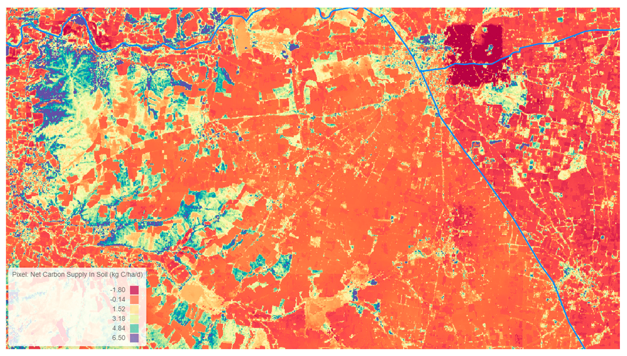
3.2.11. HESS11: Carbon Sequestration

HESS11 encompasses the water required for net intake of carbon from the atmosphere into carbon pools [100]. This is a critical process and relevant in agro-forestry environments where carbon sequestration significantly correlates with water availability and vice versa, and higher evaporation and transpiration rates reduce generated runoff [101]. Without transpiration via open stomata, CO₂ will not be captured from the air. Carbon pools consist of living above-ground biomass, living below-ground biomass, deadwood, litter and soil organic matter (SOM) [102]. Above-ground biomass comprises all organic matter (i.e., stems, branches, leaves, flowers, grains, understory and floor layers which includes herbaceous plants). The dead organic matter pool includes dead fallen plant and crop residues, the litter layer and charcoal (or partially charred organic matter) above the soil surface. The below-ground biomass comprises living and dead roots, soil fauna and the microbial community. Clearly, carbon stocks in vegetation change with land use [103]. Hairiah et al. [102] found that land use conversion can result in a positive or negative net carbon sequestration as it is related to the modification of photosynthesis.

Soil organic matter is the result of carbon humification processes and carbon decomposition into the atmosphere due to mineralization processes. The carbon from litter, stubble and roots is partially stored into the soil. Peat soils are an ultimate example of soil carbon accumulation due to lack of oxygen in flooded or stagnant water systems. Peat soils can store 10–100 times more carbon per unit area than mineral soil types and thus contribute significantly to sequester atmospheric carbon.

The estimation of carbon sequestration can come from (i) inventories based on in-situ measurements of above- and below-ground carbon stocks [86,90] and eddy-covariance flux towers (e.g., carbon flux); (ii) remote sensing algorithms for net primary production (NPP); (iii) global ecology models [104,105,106]; (iv) eco-hydrological numerical models (e.g., InVest, SWAT). IPCC AFOLU [107] is an internationally recognized framework to compute carbon stocks by land use class. ICRAF developed a database of the density of woody matters in trees (http://apps.worldagroforestry.org/sea/Products/AFDbases/WD/Index.htm (accessed on 25 October 2022)). The drawback is that every land use class has the same carbon value, while the spatial variability is significant due to differences in photosynthesis. A comprehensive overview for various methods to assess carbon pools in agricultural soils is provided by Nayak et al. [108].

The computation of pixel-dependent dry matter production and NPP from spectral radiances and land surface temperature is considered a more solid solution for making accurate assessments of carbon pools (see also HESS3 and HESS4). NPP can be subsequently used to separate carbon assimilates into (i) above ground; (ii) below ground; (iii) soil organic matter; (iv) dead wood and litter. A review of NPP models from remote sensing is provided by Sun [109]. Figure 3 illustrates an example of carbon capture calculated from NPP and humification process using remote sensing data.

3.2.12. HESS12: Reduce Greenhouse Gas Emissions

Public concern about global warming mostly focuses on carbon dioxide, the most prevalent greenhouse gas after water vapor H₂0. Methane (CH₄) is also an important greenhouse gas, yet the heating effect of an atmospheric methane increase is approximately half of a carbon dioxide increase [110,111].

The emission from various greenhouse gasses and other trace gasses depends on land use, soil moisture, air content and soil temperature. Industrial and domestic emissions are not included under HESS12. Methane emissions occur under anaerobic conditions. Inland open water such as natural lakes, ponds and reservoirs are net emitters of CH₄, N₂O and CO₂. These water bodies also play important roles in offsetting GHGs sequestered by terrestrial ecosystems [112]. Rice fields have been identified as a major source of atmospheric methane [113]. Flooding a rice field cuts off the oxygen supply from the atmosphere to the soil, which results in anaerobic fermentation of soil organic matter. Methane is a major by-product of anaerobic fermentation. It is released from submerged soils to the atmosphere by diffusion and ebullition and through the roots and stems of rice plants. Dairy farming with outdoor cows generates methane emissions while indoor cattle is also a GHG emitter because dung needs to be spread out to the environment.

HESS12 expresses reduction in greenhouse gas emissions (GHG) covering three major gases: carbon dioxide (CO₂), methane (CH₄) and nitrous oxide (N₂O). The reduction can be achieved from better water management practices, in particular proper drainage networks. Hence the depth to the water table and soil moisture below field capacity are key factors for reducing methane emissions from paddy fields and pastures.

The challenge in assessing CH₄ and N₂0 fluxes due to the lack of directly measured data can be overcome with modelling and open-source data. The dynamic land ecosystem model DLEM [114] is a good example of a mathematical framework. DLEM can be developed and implemented at pixel scale if soil moisture and soil temperature are prescribed. The determination of oil moisture was discussed under HESS8. Soil temperature derivation from earth observations has also become feasible using land surface temperatures from thermal infrared radiometers, e.g., [115,116].

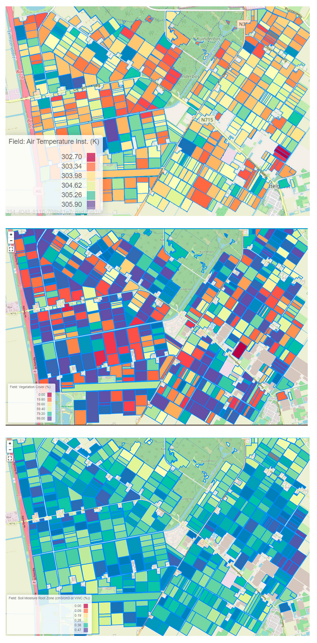
3.2.13. HESS13: Micro-Climate Cooling

The importance of micro-climates for regulating local habitats and modulating water requirements due to changing states of the near-surface atmospheric boundary layer has been recognized by various researchers [117]. Evaporating surfaces from water-dependent environments such as irrigated areas, wetlands and forested areas provide significant values in cooling the atmosphere. HESS13 describes the impact of vegetation cover on cooling of the local near-surface air mass. The lower part of the atmospheric boundary layer is per definition affected by land surface fluxes. A land surface with a high evaporative fraction (i.e., ratio of latent heat flux $\lambda E$ and net available energy $(R_n-G$)) will transport little heat into the atmosphere and the air will remain relatively cold [118]. An air mass with lower temperature from evaporating surfaces such as irrigated areas, wetlands and forested areas will impact the regional air circulation. Villages located near evaporating pastures are always cooler than villages surrounded by dryland. This is a HESS service for mankind.

The role of water on atmospheric cooling by vegetation can be best described by taking a reference situation such as a landscape without vegetation. The energy associated with evapotranspiration is 2.45 MJ/kg and this energy will no longer feed the sensible heat flux that warms up the atmosphere from the land surface. The reduction in sensible heat flux H due to ET can be expressed as a suppression of the vertical air temperature difference (T₀–T_air) yielding a colder air mass for bio-organisms and mankind in a layer of air between crops and a 2.0 m elevation at standard observation height.

Figure 4 shows an example of how the presence of vegetation and soil moisture creates many different micro-climatic conditions for an agricultural area in The Netherlands. Fields with a high leaf area index and high soil moisture are 302.7 °K while fields with lower vegetation cover are reaching 305.9 °K, hence a midday air temperature cooling of 3 °K is apparent. Note that this is air temperature at observation height and that land surface temperatures exhibit a significantly higher spatial variability (20 to 30 °K).

3.2.14. HESS14: Natural Reduction in the Eutrophication of Water

Algae are microscopic phytoplankton, such as bacteria and dinoflagellates, that use photosynthesis to turn sunlight into energy. These microorganisms are naturally occurring and live in all types of water, from fresh to salt to brackish water. When water reaches the right mix of sunlight, temperature, low water flows and excessive amounts of nutrients (e.g., eutrophication), algae can multiply very quickly and turn into a “bloom”. Nutrients, such as nitrogen and phosphorus, when in overabundance, become water pollutants and can cause super-charged algal growth. The reduction in eutrophication by sufficient flushing is considered an ecosystem service. If these algae blooms dissipate due to improved water quality upstream and sufficient flow, then natural purification processes occur.

The detection of algae dynamics in space and time can be described from remote sensing water quality data sets. MODIS has particularly designed a fluorescence band (676 nm) that can be used to detect harmful algae blooms (HAB). Water surface temperature information can be used as an additional source of information. Similarly, Landsat-8 ETM+/OLI and Sentinel-2 MSI can be used to retrieve Chl-a information [119,120]. Ma et al. [121] combined MODIS, Landsat and Sentinel images to collectively assess HAB by evaluating NDVI, floating algae index (FAI) and the chlorophyll reflection peak intensity index (${\rho }_{chl}$). Peppa et al., [122] used the maximum chlorophyll index (MCI) and maximum peak height (MPH) from Sentinel-2 to extract Chl-a information. Time series of HAB, Chl-a and phytoplankton will reveal the moments when water quality is improving; the hydrological situation at that specific moment needs to be described for understanding the amount of fresh water needed to control eutrophication.

In addition, there is a separate school assessing leaf nitrogen content as an essential indicator of N-uptake in crops. Leaf chlorophyll and nitrogen content can be best determined from red-edge (680–780 nm) reflectance. Satellite sensors such as Sentinel-2 and RapidEye can provide this information [123]. Similar studies were conducted for paddy rice [124,125] using the normalized difference red edge (NDRE) which showed a strong correlation with N present in leaves.

3.2.15. HESS15: Reduction in Soil Erosion

Wind and water create soil erosion. With increasing intensity of rainstorms, erosion is likely to occur more frequently. Erosion destroys the land surface, washes out fertile soil horizons and can be a source for landslides. Constructions are affected if soil washes away. Soil, mud and debris can lead to high-risk situations. Years of carbon sequestration in the soil can be washed out in a few hours.

Mitigation of erosion is essential, and healthy vegetation coverage is important to control soil erosion [126]. Packages of soil conservation practices exist, and they help mitigate erosion. Dang et al. [127] found that NPP was positively correlated with soil conservation. More vegetation on sloping terrain increases the infiltration of rainwater. However, vegetation for controlling soil erosion will consume water.

The universal soil loss equation (USLE) is the classical solution for determining erosion [128]. Information on slope, vegetation cover and erosivity of the soil needs to be specified. Reduction in soil erosion between vegetated landscapes and bare soil can be calculated from changes in surface runoff and applying the USLE equation for multiple conditions. Hourly or daily surface runoff values need to be computed. The soil moisture deficit is a necessity for computing surface runoff with higher accuracy [129].

3.2.16. HESS16: Meeting Environmental Flow Requirements

The provision of environmental flows is vital for maintaining specific habitats for fish, birds and plants in rivers, wetlands and estuaries. Spawning fish have, for instance, particular requirements of flow regimes. At best, the historic hydrograph under pristine conditions should be used for long term reference. This is from a period with less impact of global warming, fewer populations, catchments with higher forest cover and fewer reservoirs.

Climate change, human water withdrawals and dam constructions have a strong impact on hydrographs and can constitute a potential detriment for environmental flow requirements. While HESS14 is related to water quality through eutrophication, HESS16 describes minimum flows and minimum water levels.

There are various techniques to assess environmental flows and their condition. Xue et al. [130] quantified the environmental flow requirements (e-flows) to maintain different ecosystem functions from minimum monthly runoff. A maximum of 20% modification to a river’s natural flow is proposed by Hoekstra et al. [36] in their water scarcity analysis of 405 river basins for the period 1996–2005. When river flow deviates by more than 20% from its original discharges, it can be assumed that the environment is affected. It is not uncommon to consider flows from 50 years ago (e.g., 1960s and 1970s). Smatkhtin et al. [131], for instance, assessed the mean environmental flow requirements for 128 major basins and drainage regions worldwide using measured and simulated hydrographs. They introduced five different environmental classes and assigned fractions of the mean annual flow.

Winsemius et al. (2009) [132] and Poortinga et al. [39] developed procedures to integrate a streamflow model with remote sensing data of P, ET and soil moisture for the creation of hydrographs. Return periods of a certain f stream flow could be quickly detected, and such data are a perfect input to define flow during the 20% wettest years. Figure 5 shows the anomalies of annual runoff in the El Nino year 2009–2010 from December until February. This is a great method for utilizing earth observation data to assess environmental flow requirements.

3.2.17. HESS17: Leisure

HESS17 leisure indicates the value from socialisation and purification of humans via water sports, swimming, recreational fishing, sightseeing, aesthetic views, hiking, mountain biking, forest BBQs, etc. The common factor is that this requires water flows, water fluxes and open water bodies in pristine landscapes. While HESS16 is meant for habitats, HESS17 unravels the benefits for human satisfaction to be surrounded by pristine natural landscapes. Quantification of HESS17 can be conducted through the collection of visitor statistics of natural and urban parks. The number of leisure-oriented businesses (e.g., rental of fishboats or canoes), tourist taxes going to local communities and bars and restaurants in rural and remote areas is an indication of leisure activities.

4. Proposed HESS Determination Processes

This section describes a set of suggested formulations for HESS. The inclusion of remote sensing makes it feasible to relate hydrological processes to land use information. Various procedures based on earth observation data are summarized in

Table 2. Summary of HESS quantification methods.

Indicator	Remote Sensing Outputs	Other Quantification Methods
HESS1	P, ET, ΔS	Hydrological models
HESS2	A, H, E	FAOSTAT, WorldFish, statistics (mean annual discharge and water bodies)
HESS3	NPP	Look-up table for LULC
HESS4	NPP	Look-up table for LULC
HESS5	$B_{riv}$, H	Hydrograph measurements, rainfall-runoff models
HESS6	P, ET, ∆S, Vc	Tracers, hydrological model
HESS7	A, H	Bathymetry, gauge readings
HESS8	EF, LST, NDVI	Soil moisture and root length measurement, unsaturated zone hydrology models
HESS9	P, ET, Vc	Atmospheric models
HESS10	LU, A, H	Rainfall–runoff models
HESS11	LU, Vc, NPP	IPCC–AFOLU method
HESS12	LU, Vc, NPP	IPCC–AFOLU method
HESS13	LST, Vc, LU	Air temperature and air humidity measurements, global/regional climate model
HESS14	LU, ABDI, FAI, Chl-a, MCI, MPH, SRRE	Optical and laboratory measurement
HESS15	Vc, NPP	No. of landslides, erosion measurements
HESS16	$B_{riv}$, A, P, ET, ∆S, Vc	Historic and current hydrographs
HESS17	ET, A, H	Visitor statistics, no. of leisure businesses

.

Table 3. Summary of satellite measurements required for an operational HESS system.

Satellite	Sensor	Spatial Resolution (Nadir, m)	HESS	RS Parameters
LANDSAT	OLI-2, TIRS-2 (Landsat 9)	15–90 m	HESS3, HESS4, HESS11	EF, SM, H, NPP
	OLI, TIRS (Landsat 8)		HESS14	Chl-a, FAI, SRRE, NDRE
	ETM+ (Landsat 7)		HESS1, HESS5	Q
	MSS (Landsat 1, 2, 3)		HESS7, HESS10, HESS17	$B_{riv}$$,\mathrm{A},\Delta \mathrm{S},$Q
	TM (Landsat 4, 5)
Terra/Aqua	MODIS	250–1000 m	HESS3, HESS4, HESS11, HESS14	NPP, SRRE, NDRE, FAI
PROBA-V	Vegetation	120 m	HESS3, HESS4, HESS11	NPP
IRS	WiFS	188 m	HESS3, HESS4, HESS11	NPP
Suomi	VIIRS	375 m	HESS3, HESS4, HESS11	NPP, LST
JASON	Poseidon	na	HESS1, HESS5, HESS7, HESS10, HESS16	$\Delta \mathrm{S}$, H
Sentinel-3	Altimeter	variable	HESS1, HESS5	$\Delta \mathrm{S},\mathrm{H},$LST
Sentinel-3 Sentinel-2	Altimeter MSI	variable 10 m	HESS7, HESS10, HESS16	$\Delta \mathrm{S},\mathrm{H}$
			HESS1, HESS5	Q
Sentinel-2 Sentinel-1	MSI C-band SAR	10 m 10 m	HESS14	Vc, chl-a, FAI, NDRE
			HESS7, HESS16	$B_{riv}$, A, Q
			HESS1, HESS5	Q
Sentinel-1 ISS	C-band SAR EcoStress	10 m 70 m	HESS 8	SM
			HESS7, HESS10, HESS16	$B_{riv}$$,\mathrm{A},\Delta \mathrm{S},$Q
			HESS9, HESS13	LST, NDVI

presents the type of satellite systems.

5. Discussion

Water is by definition a multi-purpose natural resource. Its value to the environment is obvious and endless. Yet, it is also important to define limited metrics for expressing the role of water in the environment. The magnitude of ecological benefits depends on water fluxes, flows and stocks. With the presence of vegetation, there is less erosion, cooler atmospheres and less atmospheric CO₂ due to carbon capture. HESS12 considers reduced greenhouse gas emissions as the service. This implies that a reference must be defined, using either a record with sufficient monitoring of in situ measurements of hydrological features or remote sensing or through a baseline established in hydrological models. For HESS definitions focusing on changes, non-vegetated land can be taken as the reference for highlighting the contribution of hydrological regimes, such as peak flow attenuation or soil erosion. In other cases, good quality water or sufficient water for fish spawning is the reference. Hence the definition and selection of the reference is not univocal.

The determination of bio-physical processes in a spatial context and in dynamic fashion is complex. Many eco-hydrological research teams have created great analytical tools and contributed to provide insights into interactions between water resources and benefits that people and societies receive from nature. The use of eco-hydrological models plays a crucial role when it comes to better recognize and understand disturbances, land use and management and climate change scenarios. At the same time, earth observations have developed considerably during the last three decades, and the opportunities to use the growing number of open access databases on, for instance, water body occurrences, NPP and evapotranspiration should be exploited more frequently (see Table 2 and Table 3). The availability of a new sensor generation (e.g., Landsat 9, SWOT, Sentinel 3 etc.) provides more capabilities to start monitoring and reporting HESS on a regular basis, provided that an analytical framework such as HESS17 exists. The HESS framework also requires local statistical data or globally accepted data, such as FAOSTAT and WorldFISH.

The metrics of HESS17 include gross simplifications. Chlorophyll-A is, for instance, the only indicator selected for eutrophication of water bodies. The extent of firewood use as a source of daily energy does not reflect the integrated dependence of rural populations on ecosystems in low income countries. Fish catch statistics have certain limits of accuracy as the reporting process is different for each country. Figure 5 provides exciting new opportunities to fill data voids for regions without hydrographs for baseflows and fish health. However, modelled data do not have the same accuracy as flow measurements (although flow meters also contain errors). Hydro-meteorological observatories represent point measurements, and energy balance models driven by remote sensing data can help to assess fluxes and soil moisture in a truly spatially distributed context. The conclusion is that the combination of in situ measurements, remote measurements and modelling is the way forward. As an international community, we had not previously reached the technical capabilities we now have thanks to the Internet of Things.

On the other hand, despite showing great strengths and advantages, the use of spatial data sets and eco-hydrological models needs careful assessment [104]. There are limitations resulting from the complexities of climate, eco-hydrology and ecosystems, as well as interactions with human factors. Therefore, the sensitivities and limitations of these tool sets need cautious evaluation and transparent communication during the HESS quantification.

There is an imbalance in the list of HESS proposed in this manuscript, i.e., in the number of presented provisioning and regulating services as compared with cultural and support services. Evidently, this drawback results in a potential distortion while assessing the benefits of HESS to human and non-human use, as well as in the optimization of HESS performance at various scales. Further refinement of HESS definitions and categorizations is needed to minimize this ambiguity in the future. Once HESS are re-defined or more HESS are needed, the HESS framework proposed in this study can be revised and extended.

It is suggested that the integration of earth observations with eco-hydrological models is a necessary step that deserves more attention from research for the next 10 years. A good review on modelling soil as the centrepiece for environmental systems was provided by Vereecken et al. [133]. Attention should be given to the fact that integrating multiple remote sensing data sets will create noise coming from the uncertainties of each individual parameter. Error propagation should be limited by developing hydrological consistency. Schoups and Nasseri [134] describe a Bayesian hierarchical model that fuses monthly water balance data and estimates the corresponding data errors and error-corrected water balance components (precipitation, evaporation, river discharge and water storage); this type of work needs to expand for acquiring more accurate HESS values.

The HESS17 framework can be used to assess how agricultural production practices affect ecosystem services. For basin planners, the HESS framework can provide answers on how watershed management can be improved to enhance HESS. The possibility of a seamless zoom from global to regional to basin scale is crucial, not only for understanding the flow and allocation of HESS at large and “acceptable” thresholds, but also for close monitoring and managing by decision makers, as well as leveraging in policy and planning instruments.

6. Conclusions

Since the concept of ecosystem services extends across many research domains and expertise, a consistent and comprehensible approach for the quantification of HESS should be available for larger audiences. This study evaluated the status of different hydrological ecosystem services as a critical step in the planning process for sustainable development. The new HESS17 framework describes a standard list of 17 carefully defined indicators. Although not exhaustive, it is a proper balance between essential water quantity and water quality indices being presented as an integrated framework that is supported by CGIAR. In fact, HESS should be classified into consumptive use and non-consumptive use. Consumptive use leads to various services, but the water evaporated into the atmosphere is no longer available (except for local atmospheric recycling). Non-consumptive water can be reused and recycled.

The potential strengths and drawbacks of quantification methods such as remote sensing, hydrological modelling and empirical calculations are provided. Most remote sensing algorithms are meant for solving one biophysical process. The innovation of this paper is that we sketch potential procedures to integrate multiple open access data bases and remote sensing algorithms for quantifying a package of 17 standard HESS indicators. The study warns that error propagation should be controlled by recognizing the uncertainties of each parameter and seeking hydrological consistency.

Eco-hydrological models are extremely useful to estimate complex processes such as non-source pollution contaminant transport. The fusion of remote sensing and eco-hydrological models should be encouraged to establish more accurate HESS values under conditions of climate change, water scarcity and land–water–soil conservation programs. Earth observations cannot be used for future predictions, but they are useful for calibrating historic eco-hydrological processes

In conclusion, the technology and science are sufficiently mature to provide clear-cut and policy-oriented spatial information on HESS. Decades of development and new technologies in sensors, satellite platforms, data storage and computational power have resulted in advanced tools that can be used for assisting policy change by HESS implications. As the digital information era advances, future progress is expected to enable further upscaling and standardization of operational monitoring of hydrological ecosystem services.

References

1. Millennium Ecosystem Assessment (Program). Ecosystems and Human Well-Being: Wetlands and Water Synthesis: A Report of the Millennium Ecosystem Assessment; World Resources Institute: Washington, DC, USA, 2005; ISBN 978-1-56973-597-8. [Google Scholar]
2. Brauman, K.A. Hydrologic ecosystem services: Linking ecohydrologic processes to human well-being in water research and watershed management. WIREs Water 2015, 2, 345–358. [Google Scholar] [CrossRef]
3. Poortinga, A.; Nguyen, Q.; Tenneson, K.; Troy, A.; Saah, D.; Bhandari, B.; Ellenburg, W.L.; Aekakkararungroj, A.; Ha, L.; Pham, H.; et al. Linking Earth Observations for Assessing the Food Security Situation in Vietnam: A Landscape Approach. Front. Environ. Sci. 2019, 7, 186. [Google Scholar] [CrossRef] [Green Version]
4. Nature-Based Solutions for Water; UNESCO. The United Nations World Water Development Report; UNESCO: Paris, France, 2018; ISBN 978-92-3-100264-9. [Google Scholar]
5. CGIAR Research Program on Water, Land and Ecosystems (WLE). Ecosystem Services and Resilience Framework; International Water Management Institute (IWMI), CGIAR Research Program on Water, Land and Ecosystems (WLE): Colombo, Sri Lanka, 2014. [Google Scholar]
6. Bagstad, K.J.; Johnson, G.W.; Voigt, B.; Villa, F. Spatial dynamics of ecosystem service flows: A comprehensive approach to quantifying actual services. Ecosyst. Serv. 2013, 4, 117–125. [Google Scholar] [CrossRef]
7. Terrado, M.; Momblanch, A.; Bardina, M.; Boithias, L.; Munné, A.; Sabater, S.; Solera, A.; Acuña, V. Integrating ecosystem services in river basin management plans. J. Appl. Ecol. 2016, 53, 865–875. [Google Scholar] [CrossRef] [Green Version]
8. Bastiaanssen, W.; Allen, R.; Droogers, P.; D’Urso, G.; Steduto, P. Twenty-five years modeling irrigated and drained soils: State of the art. Agric. Water Manag. 2007, 92, 111–125. [Google Scholar] [CrossRef]
9. Nedkov, S.; Campagne, S.; Borisova, B.; Krpec, P.; Prodanova, H.; Kokkoris, I.P.; Hristova, D.; Le Clec’H, S.; Santos-Martin, F.; Burkhard, B.; et al. Modeling water regulation ecosystem services: A review in the context of ecosystem accounting. Ecosyst. Serv. 2022, 56, 101458. [Google Scholar] [CrossRef]
10. Schulp, C.J.; Alkemade, R.; Goldewijk, K.K.; Petz, K. Mapping ecosystem functions and services in Eastern Europe using global-scale data sets. Int. J. Biodivers. Sci. Ecosyst. Serv. Manag. 2012, 8, 156–168. [Google Scholar] [CrossRef] [Green Version]
11. Grizzetti, B.; Lanzanova, D.; Liquete, C.; Reynaud, A.; Cardoso, A.C. Assessing water ecosystem services for water resource management. Environ. Sci. Policy 2016, 61, 194–203. [Google Scholar] [CrossRef]
12. Crossman, N.D.; Burkhard, B.; Nedkov, S.; Willemen, L.; Petz, K.; Palomo, I.; Drakou, E.G.; Martin-Lopez, B.; McPhearson, T.; Boyanova, K.; et al. A blueprint for mapping and modelling ecosystem services. Ecosyst. Serv. 2013, 4, 4–14. [Google Scholar] [CrossRef]
13. Neitsch, S.; Arnold, J.; Kiniry, J.; Williams, J.R. Soil and Water Asessment Tool Theoritical Documentation: Version 2009; Texas Water Resources Institute Technical Report No. 406; Texas Water Resources Institute, Texas A&M University: College Station, TX, USA, 2011. [Google Scholar]
14. Ha, L.T.; Bastiaanssen, W.G.M.; Van Griensven, A.; Van Dijk, A.I.J.M.; Senay, G.B. Calibration of Spatially Distributed Hydrological Processes and Model Parameters in SWAT Using Remote Sensing Data and an Auto-Calibration Procedure: A Case Study in a Vietnamese River Basin. Water 2018, 10, 212. [Google Scholar] [CrossRef] [Green Version]
15. Tallis, H.; Polasky, S. Mapping and Valuing Ecosystem Services as an Approach for Conservation and Natural-Resource Management. Ann. N. Y. Acad. Sci. 2009, 1162, 265–283. [Google Scholar] [CrossRef]
16. Villa, F.; Bagstad, K.J.; Voigt, B.; Johnson, G.W.; Portela, R.; Honzák, M.; Batker, D. A Methodology for Adaptable and Robust Ecosystem Services Assessment. PLoS ONE 2014, 9, e91001. [Google Scholar] [CrossRef] [Green Version]
17. Leh, M.D.K.; Matlock, M.D.; Cummings, E.C.; Nalley, L.L. Quantifying and mapping multiple ecosystem services change in West Africa. Agric. Ecosyst. Environ. 2013, 165, 6–18. [Google Scholar] [CrossRef]
18. Hoyer, R.; Chang, H. Assessment of freshwater ecosystem services in the Tualatin and Yamhill basins under climate change and urbanization. Appl. Geogr. 2014, 53, 402–416. [Google Scholar] [CrossRef]
19. Terrado, M.; Acuña, V.; Ennaanay, D.; Tallis, H.; Sabater, S. Impact of climate extremes on hydrological ecosystem services in a heavily humanized Mediterranean basin. Ecol. Indic. 2014, 37, 199–209. [Google Scholar] [CrossRef]
20. Simons, G.; Poortinga, A.; Bastiaanssen, W.G.M.; Saah, D.S.; Troy, D.; Hunink, J.E.; de Klerk, M.; Rutten, M.; Cutter, P.; Rebelo, L.-M.; et al. On Spatially Distributed Hydrological Ecosystem Services: Bridging the Quantitative Information Gap Using Remote Sensing and Hydrological Models; FutureWater: Wageningen, The Netherlands, 2017. [Google Scholar]
21. Ha, L.T.; Bastiaanssen, W.G.M. Determination of Spatially-Distributed Hydrological Ecosystem Services (HESS) in the Red River Delta Using a Calibrated SWAT Model. Sustainability 2023, 15. in press. [Google Scholar]
22. Kumar, P. The Economics of Ecosystems and Biodiversity: Ecological and Economic Foundations; Earthscan: London, UK; Washington, DC, USA, 2010; ISBN 978-1-84971-212-5. [Google Scholar]
23. Brauman, K.A.; Daily, G.C.; Duarte, T.K.; Mooney, H.A. The Nature and Value of Ecosystem Services: An Overview Highlighting Hydrologic Services. Annu. Rev. Environ. Resour. 2007, 32, 67–98. [Google Scholar] [CrossRef]
24. Belmar, O.; Ibáñez, C.; Forner, A.; Caiola, N. The Influence of Flow Regime on Ecological Quality, Bird Diversity, and Shellfish Fisheries in a Lowland Mediterranean River and Its Coastal Area. Water 2019, 11, 918. [Google Scholar] [CrossRef] [Green Version]
25. Poff, N.L.; Richter, B.D.; Arthington, A.H.; Bunn, S.E.; Naiman, R.J.; Kendy, E.; Acreman, M.; Apse, C.; Bledsoe, B.P.; Freeman, M.C.; et al. The ecological limits of hydrologic alteration (ELOHA): A new framework for developing regional environmental flow standards: Ecological Limits of Hydrologic Alteration. Freshw. Biol. 2010, 55, 147–170. [Google Scholar] [CrossRef] [Green Version]
26. Pan, F.; Choi, W. A Conceptual Modeling Framework for Hydrologic Ecosystem Services. Hydrology 2019, 6, 14. [Google Scholar] [CrossRef] [Green Version]
27. Gao, J.; Li, F.; Gao, H.; Zhou, C.; Zhang, X. The impact of land-use change on water-related ecosystem services: A study of the Guishui River Basin, Beijing, China. J. Clean. Prod. 2017, 163, S148–S155. [Google Scholar] [CrossRef]
28. Willaarts, B.A.; Volk, M.; Aguilera, P.A. Assessing the ecosystem services supplied by freshwater flows in Mediterranean agroecosystems. Agric. Water Manag. 2012, 105, 21–31. [Google Scholar] [CrossRef]
29. Bangash, R.F.; Passuello, A.; Sanchez-Canales, M.; Terrado, M.; López, A.; Elorza, F.J.; Ziv, G.; Acuña, V.; Schuhmacher, M. Ecosystem services in Mediterranean river basin: Climate change impact on water provisioning and erosion control. Sci. Total. Environ. 2013, 458–460, 246–255. [Google Scholar] [CrossRef] [PubMed]
30. Fan, M.; Shibata, H.; Wang, Q. Optimal conservation planning of multiple hydrological ecosystem services under land use and climate changes in Teshio river watershed, northernmost of Japan. Ecol. Indic. 2016, 62, 1–13. [Google Scholar] [CrossRef]
31. Costanza, R.; D’Arge, R.; De Groot, R.; Farber, S.; Grasso, M.; Hannon, B.; Limburg, K.; Naeem, S.; O’Neill, R.V.; Paruelo, J.; et al. The value of the world’s ecosystem services and natural capital. Ecol. Econ. 1998, 25, 3–15. [Google Scholar] [CrossRef]
32. Hansen, R.; Frantzeskaki, N.; McPhearson, T.; Rall, E.; Kabisch, N.; Kaczorowska, A.; Kain, J.-H.; Artmann, M.; Pauleit, S. The uptake of the ecosystem services concept in planning discourses of European and American cities. Ecosyst. Serv. 2015, 12, 228–246. [Google Scholar] [CrossRef] [Green Version]
33. Abbas, A.; Zhao, C.; Waseem, M.; Khan, K.A.; Ahmad, R. Analysis of Energy Input–Output of Farms and Assessment of Greenhouse Gas Emissions: A Case Study of Cotton Growers. Front. Environ. Sci. 2022, 9, 826838. [Google Scholar] [CrossRef]
34. McCartney, M.; Cai, X.; Smakhtin, V. Evaluating the Flow Regulating Functions of Natural Ecosystems in the Zambezi Basin; International Water Management Institute (IWMI): Colombo, Sri Lanka, 2013. [Google Scholar]
35. Kiptala, J.K.; Mohamed, Y.; Mul, M.; van der Zaag, P. Mapping evapotranspiration trends using MODIS and SEBAL model in a data scarce and heterogeneous landscape in Eastern Africa: Mapping ET Using Modis and Sebal in a Landscape in E. Africa. Water Resour. Res. 2013, 49, 8495–8510. [Google Scholar] [CrossRef] [Green Version]
36. Hoekstra, A.Y.; Mekonnen, M.M.; Chapagain, A.K.; Mathews, R.E.; Richter, B.D. Global Monthly Water Scarcity: Blue Water Footprints versus Blue Water Availability. PLoS ONE 2012, 7, e32688. [Google Scholar] [CrossRef]
37. Perry, C.; Steduto, P.; Allen, R.G.; Burt, C.M. Increasing productivity in irrigated agriculture: Agronomic constraints and hydrological realities. Agric. Water Manag. 2009, 96, 1517–1524. [Google Scholar] [CrossRef] [Green Version]
38. Bastiaanssen, W.G.; Karimi, P.; Rebelo, L.-M.; Duan, Z.; Senay, G.; Muthuwatte, L.; Smakhtin, V. Earth Observation Based Assessment of the Water Production and Water Consumption of Nile Basin Agro-Ecosystems. Remote Sens. 2014, 6, 10306–10334. [Google Scholar] [CrossRef] [Green Version]
39. Poortinga, A.; Bastiaanssen, W.; Simons, G.; Saah, D.; Senay, G.; Fenn, M.; Bean, B.; Kadyszewski, J. A Self-Calibrating Runoff and Streamflow Remote Sensing Model for Ungauged Basins Using Open-Access Earth Observation Data. Remote Sens. 2017, 9, 86. [Google Scholar] [CrossRef] [Green Version]
40. van Eekelen, M.; Bastiaanssen, W.; Jarmain, C.; Jackson, B.; Ferreira, F.; van der Zaag, P.; Okello, A.S.; Bosch, J.; Dye, P.; Bastidas-Obando, E.; et al. A novel approach to estimate direct and indirect water withdrawals from satellite measurements: A case study from the Incomati basin. Agric. Ecosyst. Environ. 2015, 200, 126–142. [Google Scholar] [CrossRef] [Green Version]
41. Cheema, M.; Bastiaanssen, W. Land use and land cover classification in the irrigated Indus Basin using growth phenology information from satellite data to support water management analysis. Agric. Water Manag. 2010, 97, 1541–1552. [Google Scholar] [CrossRef]
42. Zad, S.N.M.; Zulkafli, Z.; Muharram, F.M. Satellite Rainfall (TRMM 3B42-V7) Performance Assessment and Adjustment over Pahang River Basin, Malaysia. Remote Sens. 2018, 10, 388. [Google Scholar] [CrossRef] [Green Version]
43. Paca, V.H.D.M.; Espinoza-Dávalos, G.E.; Hessels, T.M.; Moreira, D.M.; Comair, G.F.; Bastiaanssen, W.G.M. The spatial variability of actual evapotranspiration across the Amazon River Basin based on remote sensing products validated with flux towers. Ecol. Process. 2019, 8, 6. [Google Scholar] [CrossRef] [Green Version]
44. Sriwongsitanon, N.; Suwawong, T.; Thianpopirug, S.; Williams, J.; Jia, L.; Bastiaanssen, W. Validation of seven global remotely sensed ET products across Thailand using water balance measurements and land use classifications. J. Hydrol. Reg. Stud. 2020, 30, 100709. [Google Scholar] [CrossRef]
45. Troch, P.; Durcik, M.; Seneviratne, S.; Hirschi, M.; Teuling, A.; Hurkmans, R.; Hasan, S. New data sets to estimate terrestrial water storage change. Eos Trans. Am. Geophys. Union 2007, 88, 469–470. [Google Scholar] [CrossRef] [Green Version]
46. Simons, G.; Bastiaanssen, W.; Cheema, M.; Ahmad, B.; Immerzeel, W. A novel method to quantify consumed fractions and non-consumptive use of irrigation water: Application to the Indus Basin Irrigation System of Pakistan. Agric. Water Manag. 2020, 236, 106174. [Google Scholar] [CrossRef]
47. FAO. FAOSTAT Statistical Database; FAO: Rome, Italy, 2021. [Google Scholar]
48. Froese, R.; Pauly, D. FishBase. World Wide Web Electronic Publication; ScienceOpen, Inc.: Burlington, MA, USA, 2014. [Google Scholar]
49. FAO. The State of World Fisheries and Aquaculture 2020; FAO: Rome, Italy, 2020; ISBN 978-92-5-132692-3. [Google Scholar]
50. Welcomme, R.L. An overview of global catch statistics for inland fish. ICES J. Mar. Sci. 2011, 68, 1751–1756. [Google Scholar] [CrossRef] [Green Version]
51. Acharya, T.D.; Subedi, A.; Lee, D.H. Evaluation of Water Indices for Surface Water Extraction in a Landsat 8 Scene of Nepal. Sensors 2018, 18, 2580. [Google Scholar] [CrossRef] [PubMed] [Green Version]
52. Huang, C.; Chen, Y.; Zhang, S.; Wu, J. Detecting, Extracting, and Monitoring Surface Water From Space Using Optical Sensors: A Review. Rev. Geophys. 2018, 56, 333–360. [Google Scholar] [CrossRef]
53. Pekel, J.-F.; Cottam, A.; Gorelick, N.; Belward, A.S. High-resolution mapping of global surface water and its long-term changes. Nature 2016, 540, 418–422. [Google Scholar] [CrossRef] [PubMed]
54. Rebelo, L.-M.; Finlayson, C.M.; Strauch, A.; Rosenqvist, A.; Perennou, C.; Tøttrup, C.; Hilarides, L.; Paganini, M.; Wielaard, N.; Siegert, F.; et al. The Use of Earth Observation for Wetland Inventory, Assessment and Monitoring; An information source for Ramsar Convention on Wetlands; Secretariat of the Ramsar Convention: Gland, Switzerland, 2018; Volume 10. [Google Scholar]
55. Donlon, C.; Berruti, B.; Buongiorno, A.; Ferreira, M.-H.; Féménias, P.; Frerick, J.; Goryl, P.; Klein, U.; Laur, H.; Mavrocordatos, C.; et al. The Global Monitoring for Environment and Security (GMES) Sentinel-3 mission. Remote Sens. Environ. 2012, 120, 37–57. [Google Scholar] [CrossRef]
56. Lucas, R.; Rebelo, L.-M.; Fatoyinbo, L.; Rosenqvist, A.; Itoh, T.; Shimada, M.; Simard, M.; Souza-Filho, P.W.M.; Thomas, N.; Trettin, C.; et al. Contribution of L-band SAR to systematic global mangrove monitoring. Mar. Freshw. Res. 2014, 65, 589. [Google Scholar] [CrossRef]
57. Hortle, K.G.; Bamrungrach, P. Fisheries Habitat and Yield in the Lower Mekong River Basin; Technical Paper No. 47; Mekong River Commission Secretariat: Vientiane, Laos, 2015. [Google Scholar]
58. Reinermann, S.; Asam, S.; Kuenzer, C. Remote Sensing of Grassland Production and Management—A Review. Remote Sens. 2020, 12, 1949. [Google Scholar] [CrossRef]
59. Monteith, J.L. Solar Radiation and Productivity in Tropical Ecosystems. J. Appl. Ecol. 1972, 9, 747–766. [Google Scholar] [CrossRef] [Green Version]
60. Gómez, S.; Guenni, O.; de Guenni, L.B. Growth, leaf photosynthesis and canopy light use efficiency under differing irradiance and soil N supplies in the forage grass Brachiaria decumbens Stapf. Grass Forage Sci. 2013, 68, 395–407. [Google Scholar] [CrossRef]
61. FAO. Simple Technologies for Charcoal Making; FAO Forestry Paper; Food and Agriculture Organization of the United Nations: Rome, Italy, 1983; ISBN 978-92-5-101328-1. [Google Scholar]
62. Ahl, D.E.; Gower, S.T.; Mackay, D.S.; Burrows, S.N.; Norman, J.M.; Diak, G.R. Heterogeneity of light use efficiency in a northern Wisconsin forest: Implications for modeling net primary production with remote sensing. Remote Sens. Environ. 2004, 93, 168–178. [Google Scholar] [CrossRef]
63. Trischler, J.; Sandberg, D.; Thörnqvist, T. Estimating the Annual Above-Ground Biomass Production of Various Species on Sites in Sweden on the Basis of Individual Climate and Productivity Values. Forests 2014, 5, 2521–2541. [Google Scholar] [CrossRef] [Green Version]
64. Pukkala, T.; Pohjonen, V. Yield models for Eucalyptus globulus fuelwood plantations in Ethiopia. Biomass 1990, 21, 129–143. [Google Scholar] [CrossRef]
65. Running, S.W.; Nemani, R.R.; Hungerford, R.D. Extrapolation of synoptic meteorological data in mountainous terrain and its use for simulating forest evapotranspiration and photosynthesis. Can. J. For. Res. 1987, 17, 472–483. [Google Scholar] [CrossRef]
66. Boegh, E.; Thorsen, M.; Butts, M.; Hansen, S.; Christiansen, J.; Abrahamsen, P.; Hasager, C.; Jensen, N.; van der Keur, P.; Refsgaard, J.; et al. Incorporating remote sensing data in physically based distributed agro-hydrological modelling. J. Hydrol. 2004, 287, 279–299. [Google Scholar] [CrossRef]
67. Yang, K.; Li, M.; Liu, Y.; Cheng, L.; Duan, Y.; Zhou, M. River Delineation from Remotely Sensed Imagery Using a Multi-Scale Classification Approach. IEEE J. Sel. Top. Appl. Earth Obs. Remote Sens. 2014, 7, 4726–4737. [Google Scholar] [CrossRef]
68. Donchyts, G.; Schellekens, J.; Winsemius, H.; Eisemann, E.; Van De Giesen, N. A 30 m Resolution Surface Water Mask Including Estimation of Positional and Thematic Differences Using Landsat 8, SRTM and OpenStreetMap: A Case Study in the Murray-Darling Basin, Australia. Remote Sens. 2016, 8, 386. [Google Scholar] [CrossRef] [Green Version]
69. Bjerklie, D.M.; Birkett, C.M.; Jones, J.W.; Carabajal, C.; Rover, J.; Fulton, J.; Garambois, P.-A. Satellite remote sensing estimation of river discharge: Application to the Yukon River Alaska. J. Hydrol. 2018, 561, 1000–1018. [Google Scholar] [CrossRef] [Green Version]
70. Durand, M.; Gleason, C.J.; Garambois, P.A.; Bjerklie, D.; Smith, L.C.; Roux, H.; Rodriguez, E.; Bates, P.D.; Pavelsky, T.M.; Monnier, J.; et al. An intercomparison of remote sensing river discharge estimation algorithms from measurements of river height, width, and slope. Water Resour. Res. 2016, 52, 4527–4549. [Google Scholar] [CrossRef] [Green Version]
71. Michailovsky, C.I.; Bauer-Gottwein, P. Operational reservoir inflow forecasting with radar altimetry: The Zambezi case study. Hydrol. Earth Syst. Sci. 2014, 18, 997–1007. [Google Scholar] [CrossRef] [Green Version]
72. Schwatke, C.; Dettmering, D.; Bosch, W.; Seitz, F. DAHITI—An innovative approach for estimating water level time series over inland waters using multi-mission satellite altimetry. Hydrol. Earth Syst. Sci. 2015, 19, 4345–4364. [Google Scholar] [CrossRef] [Green Version]
73. Simons, G.; Droogers, P.; Contreras, S.; Sieber, J.; Bastiaanssen, W. Virtual Tracers to Detect Sources of Water and Track Water Reuse across a River Basin. Water 2020, 12, 2315. [Google Scholar] [CrossRef]
74. Xu, Y.; Beekman, H.E. Review: Groundwater recharge estimation in arid and semi-arid southern Africa. Hydrogeol. J. 2019, 27, 929–943. [Google Scholar] [CrossRef]
75. Wohling, D.; Petheram, C.; Leaney, F.; Jolly, I.; Crosbie, R. Review of Australian Groundwater Recharge Studies; CSIRO Australia: Canberra, Australia, 2010. [Google Scholar] [CrossRef]
76. Hessels, T.; Davids, J.C.; Bastiaanssen, W. Scalable Water Balances from Earth Observations (SWEO): Results from 50 years of remote sensing in hydrology. Water Int. 2022, 47, 866–886. [Google Scholar] [CrossRef]
77. Guo, M.; Li, J.; Sheng, C.; Xu, J.; Wu, L. A Review of Wetland Remote Sensing. Sensors 2017, 17, 777. [Google Scholar] [CrossRef] [PubMed] [Green Version]
78. Duan, Z.; Bastiaanssen, W.G.M. Evaluation of three energy balance-based evaporation models for estimating monthly evaporation for five lakes using derived heat storage changes from a hysteresis model. Environ. Res. Lett. 2017, 12, 024005. [Google Scholar] [CrossRef]
79. Hillel, D.; van Bavel, C.H.M. Simulation of Profile Water Storage as Related to Soil Hydraulic Properties. Soil Sci. Soc. Am. J. 1976, 40, 807–815. [Google Scholar] [CrossRef]
80. Wang-Erlandsson, L.; Bastiaanssen, W.G.M.; Gao, H.; Jägermeyr, J.; Senay, G.B.; van Dijk, A.I.J.M.; Guerschman, J.P.; Keys, P.W.; Gordon, L.J.; Savenije, H.H.G. Global root zone storage capacity from satellite-based evaporation. Hydrol. Earth Syst. Sci. 2016, 20, 1459–1481. [Google Scholar] [CrossRef]
81. Schmugge, T.J.; Meneely, J.M.; Rango, A.; Neff, R. Satellite microwave observations of soil moisture variations. JAWRA J. Am. Water Resour. Assoc. 1977, 13, 265–282. [Google Scholar] [CrossRef] [Green Version]
82. Jackson, T.; Le Vine, D.; Hsu, A.; Oldak, A.; Starks, P.; Swift, C.; Isham, J.; Haken, M. Soil moisture mapping at regional scales using microwave radiometry: The Southern Great Plains Hydrology Experiment. IEEE Trans. Geosci. Remote Sens. 1999, 37, 2136–2151. [Google Scholar] [CrossRef] [Green Version]
83. Woodhouse, I.H. Introduction to Microwave Remote Sensing, 1st ed.; CRC Press: Boca Raton, FL, USA, 2017; ISBN 978-1-315-27257-3. [Google Scholar]
84. Owe, M.; de Jeu, R.; Walker, J. A methodology for surface soil moisture and vegetation optical depth retrieval using the microwave polarization difference index. IEEE Trans. Geosci. Remote Sens. 2001, 39, 1643–1654. [Google Scholar] [CrossRef] [Green Version]
85. Scott, R.L.; Watts, C.; Payan, J.G.; Edwards, E.; Goodrich, D.C.; Williams, D.; Shuttleworth, W.J. The understory and overstory partitioning of energy and water fluxes in an open canopy, semiarid woodland. Agric. For. Meteorol. 2002, 114, 127–139. [Google Scholar] [CrossRef]
86. Hain, C.R.; Crow, W.T.; Mecikalski, J.R.; Anderson, M.C.; Holmes, T. An intercomparison of available soil moisture estimates from thermal infrared and passive microwave remote sensing and land surface modeling. J. Geophys. Res. 2011, 116, D15107. [Google Scholar] [CrossRef]
87. Neale, C.M.; Geli, H.M.; Kustas, W.P.; Alfieri, J.G.; Gowda, P.H.; Evett, S.R.; Prueger, J.H.; Hipps, L.E.; Dulaney, W.P.; Chávez, J.L.; et al. Soil water content estimation using a remote sensing based hybrid evapotranspiration modeling approach. Adv. Water Resour. 2012, 50, 152–161. [Google Scholar] [CrossRef]
88. Hu, G.; Jia, L. Monitoring of Evapotranspiration in a Semi-Arid Inland River Basin by Combining Microwave and Optical Remote Sensing Observations. Remote Sens. 2015, 7, 3056–3087. [Google Scholar] [CrossRef] [Green Version]
89. Carlson, T.N.; Petropoulos, G. A new method for estimating of evapotranspiration and surface soil moisture from optical and thermal infrared measurements: The simplified triangle. Int. J. Remote Sens. 2019, 40, 7716–7729. [Google Scholar] [CrossRef]
90. Yang, Y.; Guan, H.; Long, D.; Liu, B.; Qin, G.; Qin, J.; Batelaan, O. Estimation of Surface Soil Moisture from Thermal Infrared Remote Sensing Using an Improved Trapezoid Method. Remote Sens. 2015, 7, 8250–8270. [Google Scholar] [CrossRef] [Green Version]
91. FAO. WaPOR V2 Quality Assessment—Technical Report on the Data Quality of the WaPOR FAO Database Version 2; FAO: Rome, Italy, 2020; ISBN 978-92-5-133654-0. [Google Scholar]
92. Savenije, H.H. New definitions for moisture recycling and the relationship with land-use changes in the Sahel. J. Hydrol. 1995, 167, 57–78. [Google Scholar] [CrossRef]
93. van der Ent, R.J.; Savenije, H.H.G.; Schaefli, B.; Steele-Dunne, S.C. Origin and fate of atmospheric moisture over continents: Origin and fate of atmospheric moisture. Water Resour. Res. 2010, 46, W09525. [Google Scholar] [CrossRef] [Green Version]
94. Kunstmann, H.; Jung, G. Influence of soil-moisture and land use change on precipitation in the Volta Basin of West Africa. Int. J. River Basin Manag. 2007, 5, 9–16. [Google Scholar] [CrossRef]
95. Rama, H.-O.; Roberts, D.; Tignor, M.; Poloczanska, E.S.; Mintenbeck, K.; Alegría, A.; Craig, M.; Langsdorf, S.; Löschke, S.; Möller, V.; et al. Climate Change 2022: Impacts, Adaptation and Vulnerability Working Group II Contribution to the Sixth Assessment Report of the Intergovernmental Panel on Climate Change; Cambridge University Press: Cambridge, UK, 2022. [Google Scholar]
96. Elahi, E.; Khalid, Z.; Tauni, M.Z.; Zhang, H.; Lirong, X. Extreme weather events risk to crop-production and the adaptation of innovative management strategies to mitigate the risk: A retrospective survey of rural Punjab, Pakistan. Technovation 2022, 117, 102255. [Google Scholar] [CrossRef]
97. Abbas, A.; Waseem, M.; Ahmad, R.; Khan, K.A.; Zhao, C.; Zhu, J. Sensitivity analysis of greenhouse gas emissions at farm level: Case study of grain and cash crops. Environ. Sci. Pollut. Res. 2022, 29, 82559–82573. [Google Scholar] [CrossRef]
98. Elahi, E.; Khalid, Z.; Zhang, Z. Understanding farmers’ intention and willingness to install renewable energy technology: A solution to reduce the environmental emissions of agriculture. Appl. Energy 2022, 309, 118459. [Google Scholar] [CrossRef]
99. Shepherd, A.; Wu, L.; Chadwick, D.; Bol, R. A Review of Quantitative Tools for Assessing the Diffuse Pollution Response to Farmer Adaptations and Mitigation Methods Under Climate Change. In Advances in Agronomy; Elsevier: San Diego, CA, USA, 2011; Volume 112, pp. 1–54. ISBN 978-0-12-385538-1. [Google Scholar]
100. UNFCCC. Report of the Conference of Parties on Its Thirteenth Session; UNFCCC: Bali, Indonesia, 2007. [Google Scholar]
101. Khorchani, M.; Nadal-Romero, E.; Lasanta, T.; Tague, C. Carbon sequestration and water yield tradeoffs following restoration of abandoned agricultural lands in Mediterranean mountains. Environ. Res. 2022, 207, 112203. [Google Scholar] [CrossRef] [PubMed]
102. Hairiah, K. Measuring Carbon Stocks: Across Land Use Systems: A Manual; Brawijaya University and ICALRRD (Indonesian Center for Agricultural Land Resources Research and Development): Malang, Indonesia, 2011; ISBN 978-979-3198-55-2. [Google Scholar]
103. Pereira, P. Ecosystem services in a changing environment. Sci. Total. Environ. 2019, 702, 135008. [Google Scholar] [CrossRef] [PubMed]
104. Chen, L.; Wang, L.; Ma, Y.; Liu, P. Overview of Ecohydrological Models and Systems at the Watershed Scale. IEEE Syst. J. 2014, 9, 1091–1099. [Google Scholar] [CrossRef]
105. Cramer, W.; Kicklighter, D.W.; Bondeau, A.; Iii, B.M.; Churkina, G.; Nemry, B.; Ruimy, A.; Schloss, A.L.; The Participants of the Potsdam NpP Model Intercomparison. Comparing global models of terrestrial net primary productivity (NPP): Overview and key results. Glob. Chang. Biol. 1999, 5, 1–15. [Google Scholar] [CrossRef]
106. Field, C.B.; Randerson, J.T.; Malmström, C.M. Global net primary production: Combining ecology and remote sensing. Remote Sens. Environ. 1995, 51, 74–88. [Google Scholar] [CrossRef] [Green Version]
107. Eggleston, H.S.; Buendia, L.; Miwa, K.; Ngara, T.; Tanabe, K. 2006 IPCC Guidelines for National Greenhouse Gas Inventories; c/o Institute for Global Environmental Strategies IGES: Kanagawa, Japan, 2006. [Google Scholar]
108. Nayak, A.; Rahman, M.M.; Naidu, R.; Dhal, B.; Swain, C.; Tripathi, R.; Shahid, M.; Islam, M.R.; Pathak, H. Current and emerging methodologies for estimating carbon sequestration in agricultural soils: A review. Sci. Total. Environ. 2019, 665, 890–912. [Google Scholar] [CrossRef]
109. Sun, J.; Yue, Y.; Niu, H. Evaluation of NPP using three models compared with MODIS-NPP data over China. PLoS ONE 2021, 16, e0252149. [Google Scholar] [CrossRef]
110. Dickinson, R.E.; Cicerone, R.J. Future global warming from atmospheric trace gases. Nature 1986, 319, 109–115. [Google Scholar] [CrossRef] [Green Version]
111. Ramanathan, V.; Cicerone, R.J.; Singh, H.B.; Kiehl, J.T. Trace gas trends and their potential role in climate change. J. Geophys. Res. 1985, 90, 5547–5566. [Google Scholar] [CrossRef] [Green Version]
112. Mondal, B.; Bauddh, K.; Kumar, A.; Bordoloi, N. India’s Contribution to Greenhouse Gas Emission from Freshwater Ecosystems: A Comprehensive Review. Water 2022, 14, 2965. [Google Scholar] [CrossRef]
113. Cicerone, R.J.; Shetter, J.D. Sources of atmospheric methane: Measurements in rice paddies and a discussion. J. Geophys. Res. 1981, 86, 7203. [Google Scholar] [CrossRef] [Green Version]
114. Tian, H.; Xu, X.; Liu, M.; Ren, W.; Zhang, C.; Chen, G.; Lu, C. Spatial and temporal patterns of CH4 and N2O fluxes in terrestrial ecosystems of North America during 1979–2008: Application of a global biogeochemistry model. Biogeosciences 2010, 7, 2673–2694. [Google Scholar] [CrossRef] [Green Version]
115. Huang, R.; Huang, J.-X.; Zhang, C.; Ma, H.-Y.; Zhuo, W.; Chen, Y.-Y.; Zhu, D.-H.; Wu, Q.; Mansaray, L.R. Soil temperature estimation at different depths, using remotely-sensed data. J. Integr. Agric. 2020, 19, 277–290. [Google Scholar] [CrossRef]
116. Xu, C.; Qu, J.J.; Hao, X.; Zhu, Z.; Gutenberg, L. Surface soil temperature seasonal variation estimation in a forested area using combined satellite observations and in-situ measurements. Int. J. Appl. Earth Obs. Geoinf. 2020, 91, 102156. [Google Scholar] [CrossRef]
117. van Woesik, F. Micro-Climate Management. DownToEarth 2022, in press. [Google Scholar]
118. Osann Jochum, M.A. Operational Space-Assisted Irrigation Advisory Services: Overview of and Lessons Learned from the Project DEMETER. In Proceedings of the AIP Conference Proceedings, Naples, Italy, 10–11 November 2005; Volume 852, pp. 3–13. [Google Scholar] [CrossRef] [Green Version]
119. Dörnhöfer, K.; Klinger, P.; Heege, T.; Oppelt, N. Multi-sensor satellite and in situ monitoring of phytoplankton development in a eutrophic-mesotrophic lake. Sci. Total. Environ. 2018, 612, 1200–1214. [Google Scholar] [CrossRef]
120. Poddar, S.; Chacko, N.; Swain, D. Estimation of Chlorophyll-a in Northern Coastal Bay of Bengal Using Landsat-8 OLI and Sentinel-2 MSI Sensors. Front. Mar. Sci. 2019, 6, 598. [Google Scholar] [CrossRef]
121. Ma, J.; Jin, S.; Li, J.; He, Y.; Shang, W. Spatio-Temporal Variations and Driving Forces of Harmful Algal Blooms in Chaohu Lake: A Multi-Source Remote Sensing Approach. Remote Sens. 2021, 13, 427. [Google Scholar] [CrossRef]
122. Peppa, M.; Vasilakos, C.; Kavroudakis, D. Eutrophication Monitoring for Lake Pamvotis, Greece, Using Sentinel-2 Data. ISPRS Int. J. Geo-Inf. 2020, 9, 143. [Google Scholar] [CrossRef] [Green Version]
123. Sharifi, A. Using Sentinel-2 Data to Predict Nitrogen Uptake in Maize Crop. IEEE J. Sel. Top. Appl. Earth Obs. Remote Sens. 2020, 13, 2656–2662. [Google Scholar] [CrossRef]
124. Kanke, Y.; Tubaña, B.; Dalen, M.; Harrell, D. Evaluation of red and red-edge reflectance-based vegetation indices for rice biomass and grain yield prediction models in paddy fields. Precis. Agric. 2016, 17, 507–530. [Google Scholar] [CrossRef]
125. Zhang, K.; Ge, X.; Shen, P.; Li, W.; Liu, X.; Cao, Q.; Zhu, Y.; Cao, W.; Tian, Y. Predicting Rice Grain Yield Based on Dynamic Changes in Vegetation Indexes during Early to Mid-Growth Stages. Remote Sens. 2019, 11, 387. [Google Scholar] [CrossRef] [Green Version]
126. Pereira, P.; Bogunovic, I.; Muñoz-Rojas, M.; Brevik, E.C. Soil ecosystem services, sustainability, valuation and management. Curr. Opin. Environ. Sci. Health 2018, 5, 7–13. [Google Scholar] [CrossRef]
127. Dang, Y.; Ren, W.; Tao, B.; Chen, G.; Lu, C.; Yang, J.; Pan, S.; Wang, G.; Li, S.; Tian, H. Climate and Land Use Controls on Soil Organic Carbon in the Loess Plateau Region of China. PLoS ONE 2014, 9, e95548. [Google Scholar] [CrossRef] [Green Version]
128. Williams, J.R. The EPIC Model. In Computer Models of Watershed Hydrology; Water Resources Publications: Littleton, CO, USA, 1995; pp. 909–1000. [Google Scholar]
129. Schaake, J.C.; Koren, V.I.; Duan, Q.; Mitchell, K.; Chen, F. Simple water balance model for estimating runoff at different spatial and temporal scales. J. Geophys. Res. Atmos. 1996, 101, 7461–7475. [Google Scholar] [CrossRef]
130. Xue, J.; Gui, D.; Zhao, Y.; Lei, J.; Feng, X.; Zeng, F.; Zhou, J.; Mao, D. Quantification of Environmental Flow Requirements to Support Ecosystem Services of Oasis Areas: A Case Study in Tarim Basin, Northwest China. Water 2015, 7, 5657–5675. [Google Scholar] [CrossRef] [Green Version]
131. Smakhtin, V.; Revenga, C.; Döll, P. A Pilot Global Assessment of Environmental Water Requirements and Scarcity. Water Int. 2004, 29, 307–317. [Google Scholar] [CrossRef]
132. Winsemius, H.C.; Schaefli, B.; Montanari, A.; Savenije, H.H.G. On the calibration of hydrological models in ungauged basins: A framework for integrating hard and soft hydrological information: Integrating hard and soft information. Water Resour. Res. 2009, 45, W12422. [Google Scholar] [CrossRef] [Green Version]
133. Vereecken, H.; Schnepf, A.; Hopmans, J.; Javaux, M.; Or, D.; Roose, T.; Vanderborght, J.; Young, M.; Amelung, W.; Aitkenhead, M.; et al. Modeling Soil Processes: Review, Key Challenges, and New Perspectives. Vadose Zone J. 2016, 15, 1–57. [Google Scholar] [CrossRef] [Green Version]
134. Schoups, G.; Nasseri, M. GRACEfully Closing the Water Balance: A Data-Driven Probabilistic Approach Applied to River Basins in Iran. Water Resour. Res. 2021, 57, e2020WR029071. [Google Scholar] [CrossRef]
Figure 1. Changes in the water level of the White Nile near Kodok in South Sudan measured by the altimeter on Sentinel-3A. Base flow is pertinent when the water level is at approximately 385.4 m AMSL (source Dahiti, Technical University of Munich) (http://dahiti.dgfi.tum.de/11745/, accessed on 25 October 2022) [66].
Sustainability 15 06182 g001
Figure 2. Probability of water occurrences in Easoup Thuong reservoir, central Vietnam, based on satellite images of the open area. During wet periods, the area doubles in size.
Sustainability 15 06182 g002
Figure 3. Carbon capture of an agricultural landscape with smallholders in Madyha Pradesh (India) computed from remote sensing algorithms of NPP and a humification process.
Sustainability 15 06182 g003
Figure 4. Example of midday air temperature on a field-by-field basis in the Noordoostpolder (The Netherlands) on 12 August 2020 based on actual vegetation cover and soil moisture conditions.
Sustainability 15 06182 g004
Figure 5. Anomalies of surface runoff during El Nino. Areas with reduced and enhanced stream flow can be seen. This information can be used to check whether environmental flow requirements are met [39].
Sustainability 15 06182 g005