
Evaluating the Urban-Rural Differences in the Environmental Factors Affecting Amphibian Roadkill
by
 and
and
Jingxuan Zhao
1,2,
Weiyu Yu
1,2,3,*,
Kun He
1,
Kun Zhao
1,2,
Chunliang Zhou
1,2,
Jim A. Wright
3 and
Fayun Li
1,2,* 1
School of Ecological Technology and Engineering, Shanghai Institute of Technology, Fengxian Campus, Shanghai 201418, China
2
Center for Urban Road Ecological Engineering and Technology of Shanghai Municipality, Shanghai 201418, China
3
School of Geography and Environmental Science, University of Southampton, Building 44, Highfield, Southampton SO17 1BJ, UK
*
Authors to whom correspondence should be addressed.
Sustainability 2023, 15(7), 6051; https://doi.org/10.3390/su15076051
Submission received: 16 February 2023
/
Revised: 23 March 2023
/
Accepted: 29 March 2023
/
Published: 31 March 2023
(This article belongs to the Special Issue Biodiversity and Ecosystem Services in Agriculture, Forestry and Urban Ecosystems)
Abstract
:Roads have major impacts on wildlife, and the most direct negative effect is through deadly collisions with vehicles, i.e., roadkill. Amphibians are the most frequently road-killed animal group. Due to the significant differences between urban and rural environments, the potential urban-rural differences in factors driving amphibian roadkill risks should be incorporated into the planning of mitigation measures. Drawing on a citizen-collected roadkill dataset from Taiwan island, we present a MaxEnt based modelling analysis to examine potential urban-rural differences in landscape features and environmental factors associated with amphibian road mortality. By incorporating with the Global Human Settlement Layer Settlement Model—an ancillary human settlement dataset divided by built-up area and population density—amphibian roadkill data were divided into urban and rural data sets, and then used to create separate models for urban and rural areas. Model diagnostics suggested good performance (all AUCs > 0.8) of both urban and rural models. Multiple variable importance evaluations revealed significant differences between urban and rural areas. The importance of environmental variables was evaluated based on percent contribution, permutation importance and the Jackknife test. According to the overall results, road density was found to be important in explaining the amphibian roadkill in rural areas, whilst precipitation of warmest quarter was found to best explain the amphibian roadkill in the urban context. The method and outputs illustrated in this study can be useful tools to better understand amphibian road mortality in urban and rural environments and to inform mitigation assessment and conservation planning.
1. Introduction
Roads are the largest linear infrastructures in the world and have become integral components of human society that connect productive places for transportation of people and resources on a daily basis. The expanding road networks have dramatically altered the landscape [1], and have both direct and indirect impacts on wildlife [2], including the fragmentation and loss of habitat [1], disturbance via noise and pollution [3], and direct mortality through wildlife-vehicle collisions when wild animals cross roads. In countries with available data, wildlife deaths caused by road traffic account for millions of wildlife mortalities every year [4]. Among these, amphibians are particularly susceptible to deadly collisions with vehicles [2,5] because of their unique traits, such as breeding migrations, slow movement speed [6], limited behavioural response to oncoming vehicles [7,8], and because they are often too small in size for drivers to observe and avoid [9]. For certain local individual species, the death rate due to road traffic may exceed the normal death rate due to predation or disease [10,11]. In a global context, amphibians are among the most seriously declining animal groups [12], and roadkill has been recognised as one of the main drivers [13,14,15].
Amphibian species play prominent social-ecological roles in the ecosystem [16], as they contribute to energy transfer, nutrient cycling, and primary production, which in turn help to maintain ecosystem services and shape ecological communities [17]. In comparison with other organisms, amphibians have the unique function of their biological and ecological characteristics changing with changes of the ecological environment. They are therefore more sensitive to certain conditions in the environment, and can be used as an important indicator group for ecological environment monitoring [18,19]. In a context of extinctions and population declines globally [20], it is therefore vital to mitigate road impacts and maintain the amphibian population for ecosystem health and sustainability.
In response to growing concern over amphibian road mortality, a series of studies has been carried out, and various mitigation measures have recently been proposed. Such mitigation measures include, for example, road-crossing structures such as fence and tunnel systems [21,22], habitat replacement/improvement [6,21], as well as enforced speed limits and traffic restrictions [23]. Planning of such mitigation measures requires understanding of the relationships between amphibian roadkill patterns and environmental characteristics so as to identify potential areas with elevated risks as targets. However, due to significant urban-rural differences in the environment and the urban landscape, the response of environmental characteristics to the roadkill risks may vary between urban and rural areas [24]. As such, conventional mitigation measures may not be universally applicable in urban and rural areas. So far, the majority of previous studies on environmental drivers of roadkill risks have been carried out only in rural areas or nature reserves [25,26,27,28]. Despite the prominent social-ecological roles of amphibians in the urban ecosystem and the importance of maintaining their urban populations for ecosystem health and sustainability [16], relevant studies on amphibian road mortality for urban contexts remain limited. There is thus an emerging need for an understanding of amphibian roadkill that differentiates the rural and urban environments to inform mitigation planning accordingly.
The majority of previous studies examining the relationships between amphibian roadkill patterns and environmental characteristics are often carried out at local scales [9,29,30], and knowledge of the differences between urban and rural contexts is also scant. In addition, conventional density-based methodologies looking at environmental drivers of wildlife roadkill [30,31,32] rely heavily on routine survey data, and thus are often restricted to the local scale. Taking advantage of the potential large spatial coverage of citizen-science dataset, we therefore present a large-scale case study looking at the urban-rural differences in the environmental factors of amphibian roadkill. Taiwan island was selected as a case study given the availability of amphibian roadkill data from a citizen-science project. In our study, we resort to a novel method that is appropriate for large spatial scales proposed in previous studies to analyse and predict collision risk by modelling hazard (presence and movement of vehicles) and exposure (animal presence) across geographic space [33]. Based on an environmental niche modelling method, roadkill data for amphibians in urban and rural areas were analysed separately. The main objectives of this study are to (1) analyse the major environmental factors that may potentially explain the distribution of amphibian roadkill on Taiwan island; (2) examine the difference in environmental factors affecting amphibian roadkill risk between urban and rural areas, or potential insights to facilitate mitigation planning; and (3) examine the potential applicability of the MaxEnt modelling method for understanding amphibian response to exposure to vehicle collisions using roadkill observations.
2. Materials and Methods
2.1. Study Area and Roadkill Data
Taiwan island (20°45′2″–25°56′30″ N, 119°18′03″–124°34′30″ E) is a subtropical island located approximately 130 km off the south-eastern coast of mainland China. The great variation in topography on Taiwan island leads to changes in climate and habitat, which in turn results in great amphibian biodiversity. The amphibian-rich Taiwan island currently has over 40 known amphibian species [34], characterised by high levels of endemism [35] as well as their great importance in the local ecosystem [36]. Whilst most of the endemic amphibians have very restricted geographic distribution ranges [34], their contact areas often offer valuable opportunities for evolutionary studies [35]. With a total area of 36,000 km2, the geographic landscape of Taiwan island is predominantly rural and mountainous. Nevertheless, Taiwan island has a population of approximately 23 million, making it a densely populated island with a dense road network [37]. The highway network in Taiwan island, for example, has a total length of approximately 21,000 km [38] and is twice the road density of the U.S.A. [39].
Data on amphibian roadkill locations were obtained from the Taiwan Roadkill Observation Network (TaiRON) database via the Global Biodiversity Information Facility (GBIF; https://www.gbif.org/; accessed on 1 May 2021). The TaiRON is a citizen-science project run by the Taiwan Endemic Species Research Institute and Institute of Information Science, covering over 60,000 roadkill sightings and other animal mortality incidents throughout Taiwan since 2011. Spotted road-killed animals are reported by citizen-scientists via the TaiRON App or website to generate the roadkill data which covers observation time, geography, and species information, alongside a photo. For all incidents, species identification is verified by project managers for accuracy, which are then either marked as “confirmed” or “unable to confirm”. “Confirmed” observations will be published on TaiRON’s website and/or via other portals such as the GIBF. Following the TaiRON protocol, roadkill carcasses were removed from the road once recorded to prevent the risk of double-counting.
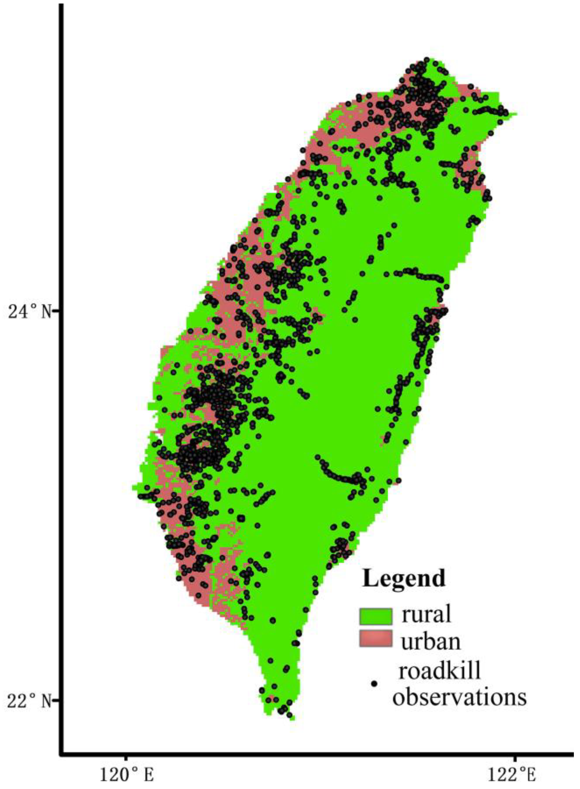
In this study, the TaiRON dataset obtained from the GBIF contained a total of 46,416 observations with a temporal coverage of 2011–2017. We restricted our analysis to amphibian species as a whole, excluding data on other non-amphibian species as well as those with unclear or no taxon information. We further excluded data with incomplete geographic information, unreasonable locations (e.g., outside the study area), and we divided pre-processed roadkill data into urban-rural sets with reference to the Global Human Settlement Layer Settlement model (GHSL SMOD) data product acquired from the European Union, European Commission (https://ghsl.jrc.ec.europa.eu/; accessed on 4 November 2021). It delineates settlement typologies based on population size for cell clusters, population and built-up area densities, and classifies areas with a density of at least 300 inhabitants per km2 of permanent land, a built-up surface share on permanent land greater than 0.03, and at least 5000 inhabitants as urban areas, with the remainder classified as rural areas. An urban-rural map of the study area and pre-processed amphibian roadkill locations is shown in Figure 1.
2.2. Environmental Variables
Similar to many large-scale representative studies using species distribution modelling, our analysis was spatial rather than spatio-temporal, given the small quantity of our derived roadkill samples for early years (i.e., 2011, 2012, etc.). Our selection of candidate environmental variables was based upon a previous study [33] where roadkill risk was expressed as a function of ‘exposure’ (i.e., species presence) and ‘hazard’ (animal-vehicle collision). For predictive variables reflecting the ‘exposure’ aspect (i.e., potential amphibian distribution), we included the 19 bioclimatic variables derived from the WorldClim database (http://www.worldclim.org; accessed on 23 May 2021), since previous studies have linked them to potential distributions of amphibian species [40,41]. In addition, we included the Normalized Difference Vegetation Index (NDVI) as an additional environmental variable since it has been used as a successful predictor of the amphibian species richness [42], and the biological characteristics of vertebrates, including species richness, abundance and distribution, and landscape connectivity [27,43,44,45]. We calculated the average NDVI derived from the MODIS/Terra Vegetation Indices Monthly L3 Global 1 km SIN Grid V006 (MOD13A3v006), obtained from the Level-1 and Atmosphere Archive and Distribution System Distributed Active Archive Center (LAADS DAAC) website (https://ladsweb.modaps.eosdis.nasa.gov/; accessed on 19 September 2021). Calculation of the average NDVI was carried out using MOD13A3v006 data in 2011–2017 for temporal matching between the MOD13A3v006 data and the obtained TaiRON roadkill data. We further included the altitude given its value in studying animal roadkill [46] and amphibian diversity and distribution [47]. The environmental variable depicting altitude was derived from the 30 m resolution Digital Elevation Model (DEM) obtained from the Geospatial Data Cloud portal (http://www.gscloud.cn/search; accessed on 8 May 2021). Furthermore, we included the density of waterways as it may also affect amphibian roadkill [30,48]. The density of waterway was calculated using OpenStreetMap-derived data in ArcGIS 10.4.1 (ESRI, Redlands, USA). For predictive variables reflecting the ‘hazard’ aspect, we included road density, as it is closely linked to the risk of amphibian-vehicle collision [34,49]. We employed road density by road types to reflect traffic speed and volume, since currently existing large-scale data sources on road traffic are limited. Road density variables were calculated using road polyline data derived from the OpenStreetMap portal (https://www.openstreetmap.org/; accessed: 9 May 2021), including the road density of motorways, primary roads, secondary roads and tertiary roads, and total road density. All candidate environmental variables (Table 1) were prepared at a spatial resolution of 30 arc-seconds (approximately 1 km at the equator) using the same spatial extent for all layers. To reduce multicollinearity, predictor variables that had a strong correlation in a pairwise matrix were identified using the Pearson correlation coefficient (r), where |r| ≥ 0.7 were considered strongly correlated, following a previous study [50]. The variable in each pair that was easiest to interpret in subsequent analysis, and/or least correlated with all other environmental variables, was retained. All data preprocessing and spatial analysis were performed in the ArcGIS 10.4.1 software (ESRI, Redlands, USA).
2.3. Data Analysis
Species distribution modelling (SDM) is an important tool for conservation planning and theoretical research on spatial ecology [51]. Conventional SDM methods such as Boosted Regression Trees (BRT) [52], Random Forest (RF) [53], and Maximum Entropy Models (MaxEnt) [54] have been adopted in various applications concerning wildlife roadkill [33,55,56]. In this study, we employed the MaxEnt as it has embedded the Jackknife test for predictor variable contribution and is considered one of the most robust and widely used SDMs [57] in the studies of roadkill. The MaxEnt optimises species-environment associations using multiple function types, including functions and product quadratic [58], and thus is especially useful in mapping ecological phenomena that may have complex non-linear correlations.
In contrast to conventional approaches where the urban-rural gradient was defined by environmental variables, we created separate models for amphibian roadkill in rural and urban areas, so as to find potentially differing functions for roadkill-environment relationships between rural and urban areas algorithmically. We employed training-test Area Under the Receiver Operator Curve (AUC) differences as a measure of potential model overfitting; our models, therefore, were developed utilising the framework of the Monte Carlo cross-validation (MCCV) [59], given the sufficiency of the obtained amphibian roadkill sample. For each model, the occurrence dataset was randomly split into two groups to create a training sample (70%) for model fitting, and a test sample (30%) for predictive performance evaluation [55]. To select specific model settings approximating optimal levels of complexity, we made models with a wide variety of different combinations of feature classes (FC: Linear; Linear and Quadratic; Linear and Hinge; Linear and Product; Linear, Quadratic and Product; Linear, Quadratic, Product and Hinge) and regularization multipliers (RM: 0.5–5.0 with 0.5 intervals). We included all reasonable features in the models to capture the potential non-linear relationships between roadkill risk and environmental drivers, and we let the algorithm detect which best fit the data via regularisation, following the practical guidance on MaxEnt modelling [58].
We then used the sample size corrected Akaike’s Information Criterion (AICc) [60] to rank models and to select the simplest model with the greatest predictive performance. The subsampling and model fitting were repeated 100 times to generate summarised outputs of environmental variable contribution and performance evaluation for urban and rural areas, respectively. To control for potential sampling bias in the opportunistic observation records derived from the TaiRON roadkill dataset, we calculated the kernel density separately using urban and rural roadkill data, and then took the kernel density layers as probabilistic weights for randomly generating pseudo-absence sample points within rural and urban areas, respectively, following previous studies [61]. The kernel density calculates a magnitude per grid from the roadkill sample points based upon a kernel function to fit a smoothly tapered surface on top of the samples, which allows the randomly generated pseudo-absence samples to be geographically clustered around these sample data. In doing so, the random sampling of pseudo-absence simulated a scenario whereby areas close to observed roadkill samples received greater survey effort than more distant areas, thereby minimising potential sampling bias as far as possible. We generated 10,000 pseudo-absence samples for rural areas and 5000 for urban areas (since it covers only 5331 grid cells in total).
The importance of environmental variables was evaluated based on the changes in regularised gains (percent contribution; PC), and changes in AUC (normalised to give percentages) based on permuted data (permutation importance; PI), alongside the embedded Jackknife test. The Jackknife test excludes environmental variables in turn when running the model, and determines variable importance by evaluating the performance of the model built without an environmental variable, as well as the model built using only that environmental variable [62]. An environmental variable is considered most important when the model excludes the variable that has the largest AICc value, or when the model built solely with this environmental variable used in isolation has the smallest AICc value. We examined multiple metrics to variable importance, and the most important variable was that identified as such by the metrics, since there was no ‘gold standard’ metric to examine how each environmental variable influenced roadkill risks.
We plotted the response curves of the environmental variables for all 100 replicated runs and fitted a trend line based on LOESS (Local Regression) smoothing for both urban and rural models, since this portrays potential complicated non-linear relationships. Each of the response curves was created by generating a model using only the corresponding environmental variable and disregarding all other variables.
The predictive performance of the models was assessed using the AUC [63]. The AUC value lies between 0.5 and 1, where the predictive power can be considered excellent (AUC ≥ 0.9), good (0.8 ≤ AUC < 0.9), fair (0.6 ≤ AUC < 0.8), and poor (AUC < 0.6), respectively [64]. The format of model output was kept as cloglog as default, indicating a relative ranking of roadkill risks within each model. We did not adopt an optimal cut-off value for urban-rural comparison between models, as our objective was to identify urban-rural differences in the ranking of environmental drivers. All analysis was carried out in R 4.1.2 (R Core Team 2021). Spatial analysis was performed using the ‘sp’ package [65,66], whilst model fitting was accomplished using the ‘SDMtune’ package [67].
3. Results
3.1. Roadkill Summary
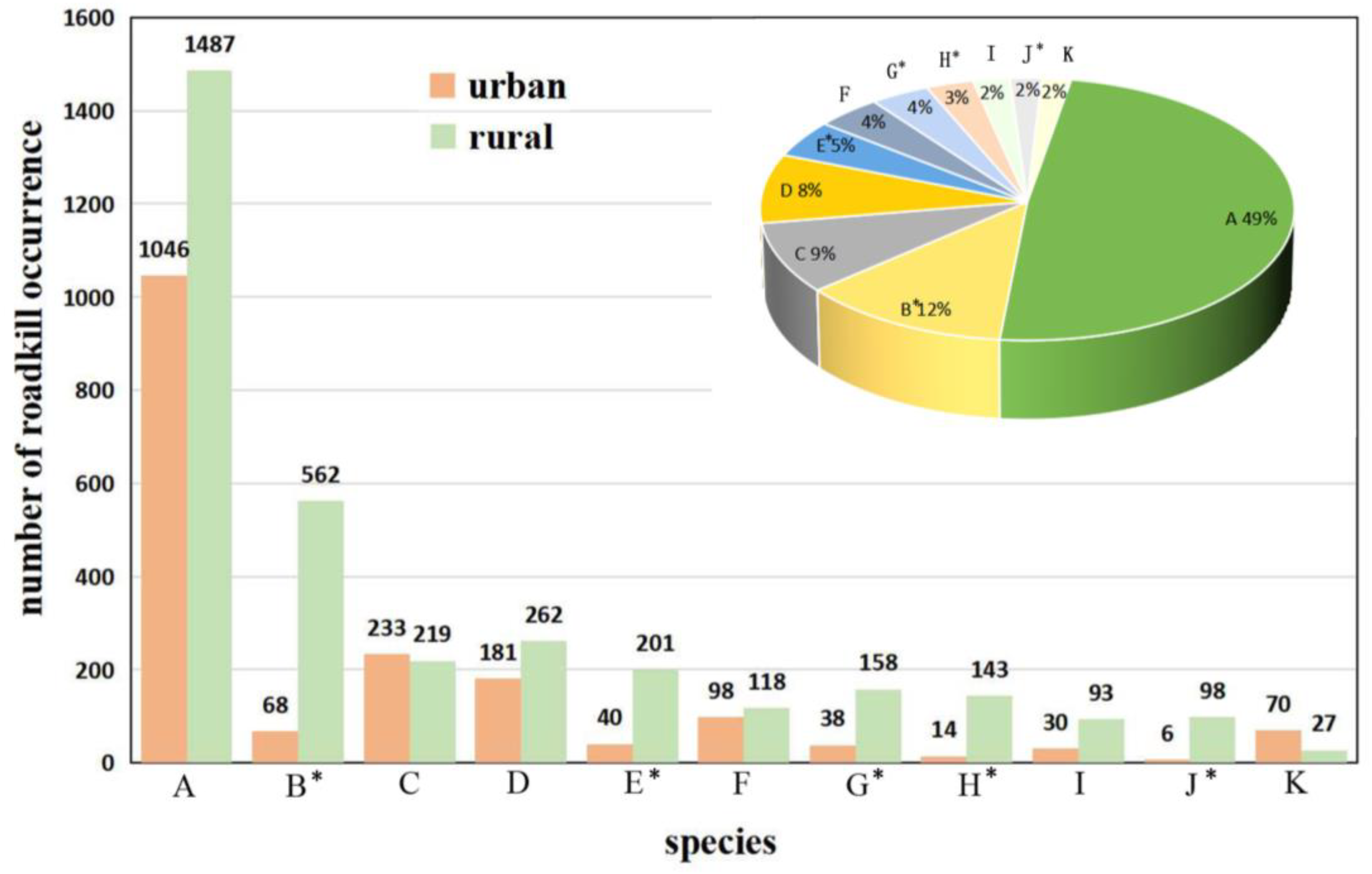
The screened data from the TaiRON dataset contained 5192 roadkill observations of 11 amphibian species from 5 families. Of these, as shown in Figure 2, 1824 records were collected from urban areas and 3368 from rural areas, and the number of roadkill varied by species. The most frequently observed road-killed amphibian species are the Asian Common toad (Bufo melanostictus), a kind of toad with medicinal properties, which roughly accounted for one-half of the total. The second most common is the Central Formosan toad (Bufo bankorensis), which is around eight times more abundant in rural areas than in urban areas. These two species are the only two species of the Bufonidae genus in Taiwan [68]. The third most common is the Common Asian Grassfrog (Fejervarya limnocharis), with numbers in rural and urban areas being not much different. The fewest roadkill observations were of the Upland Treefrog (Polypedates braueri), which is more common in urban areas than rural ones; except for this species, roadkill samples of other species were found more frequently in rural than urban areas. In addition, Chinese Bull frog (Buergeria robusta), Swinhoe’s frog (Odorrana swinhoana), and Central Formosan toad (Bufo bankorensis) are endemic to Taiwan island.
3.2. Model Outputs
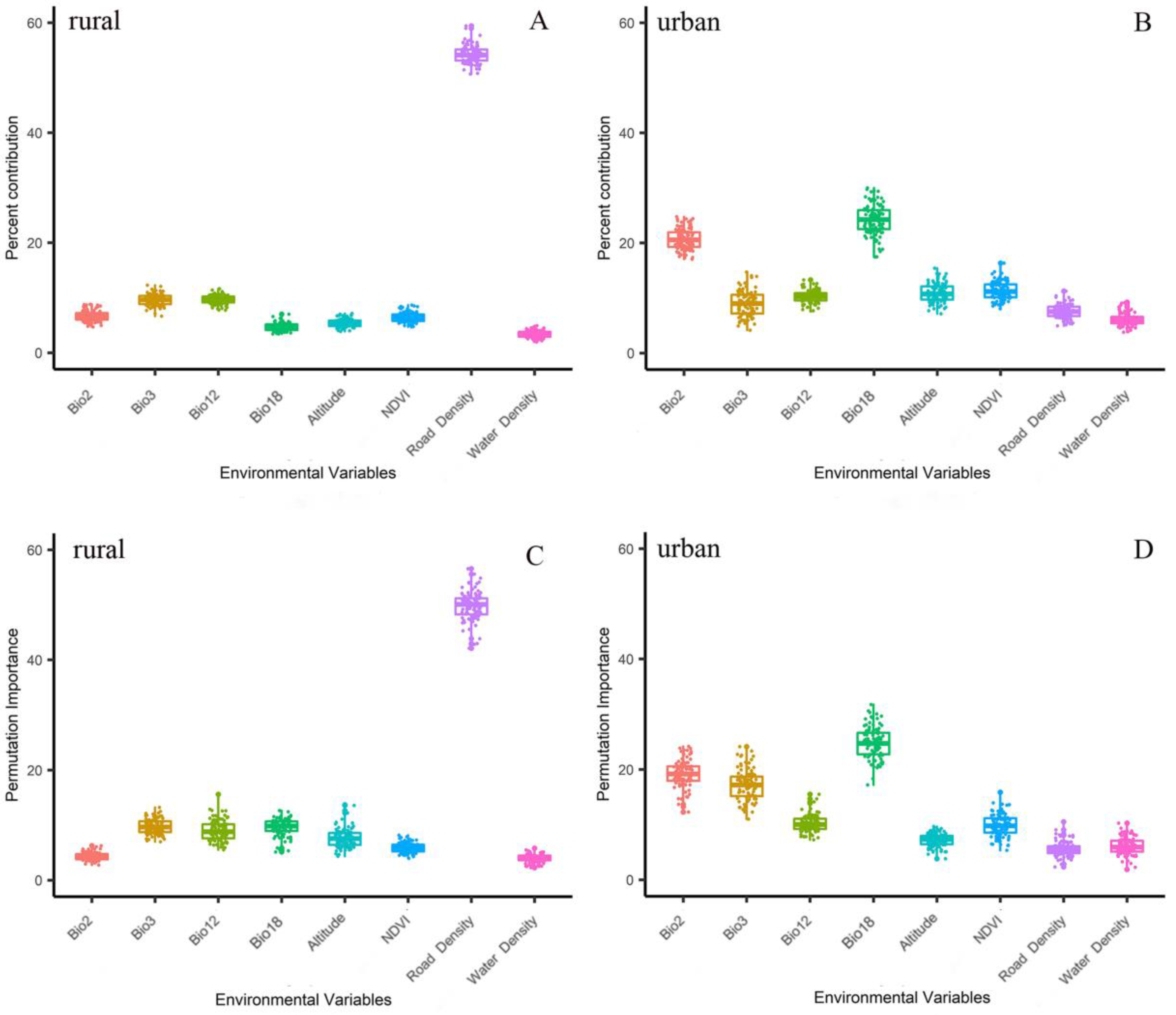
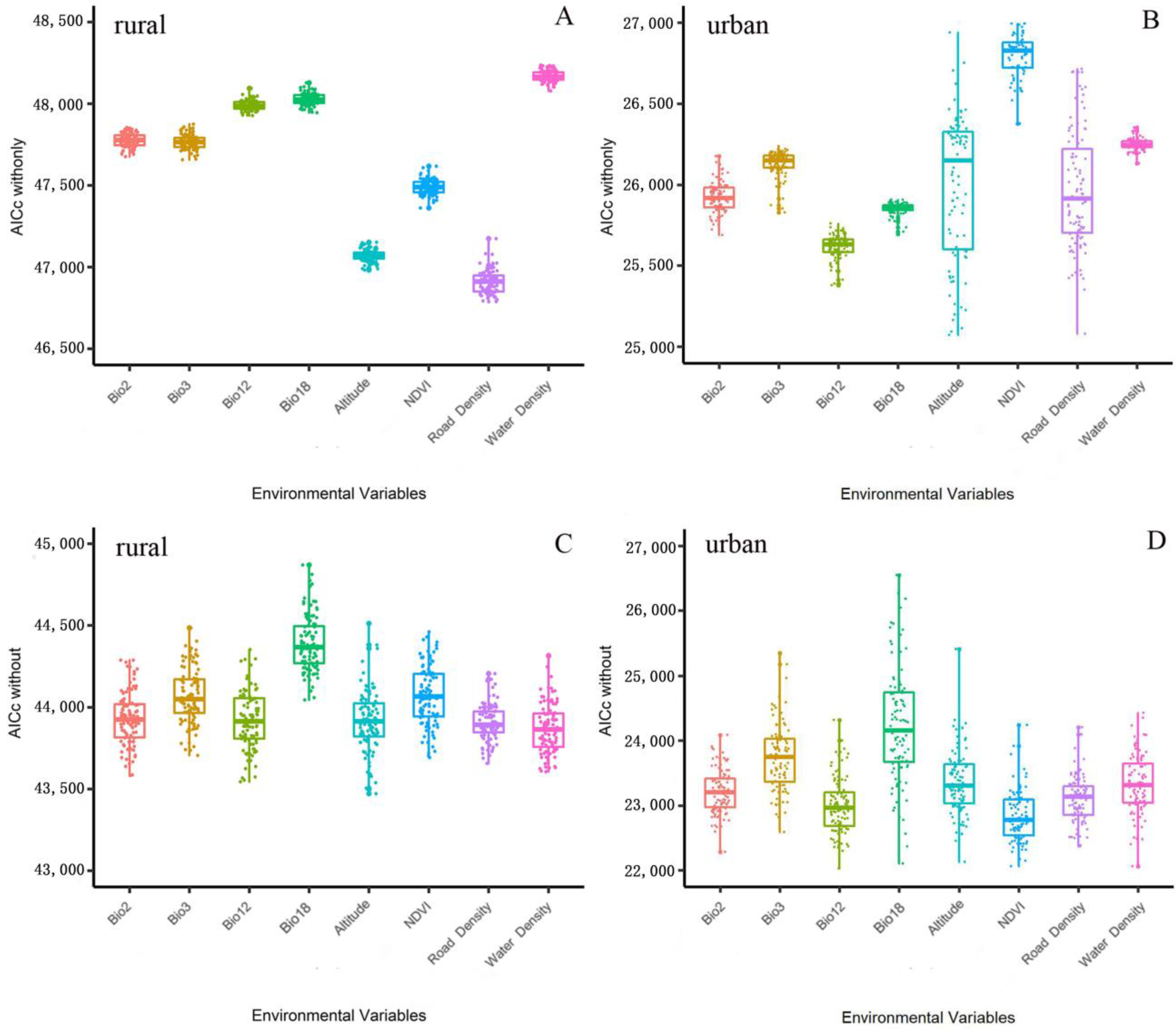
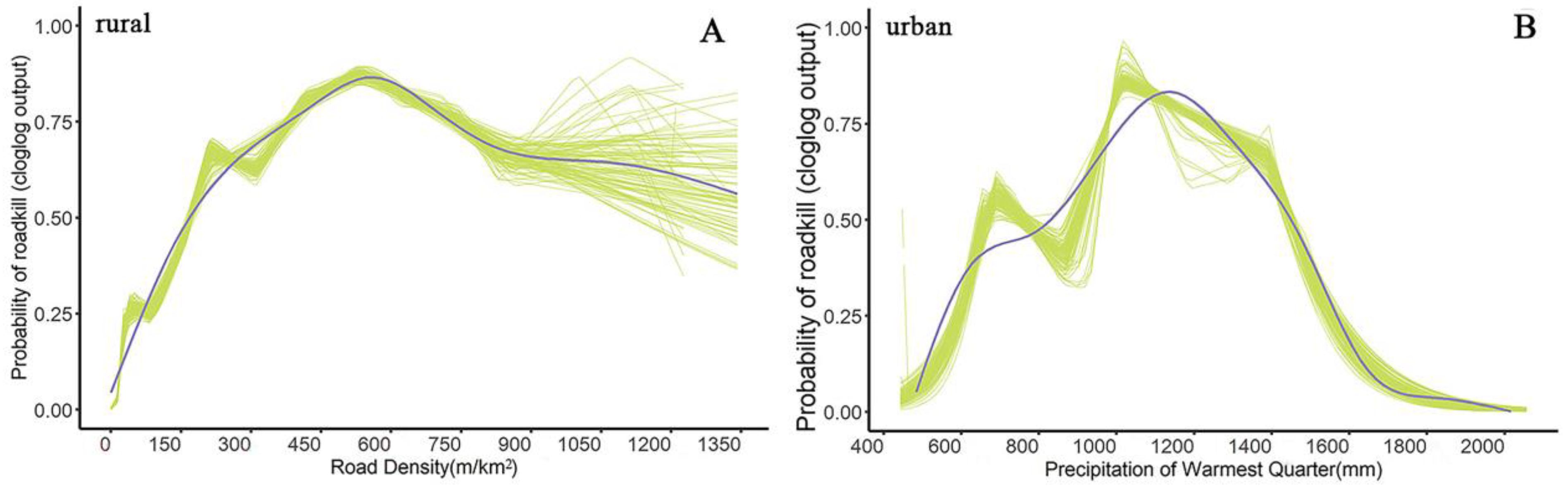
Eight environmental variables were selected for inclusion in our modelling analysis based on their pairwise correlations (Table S1), including Mean Diurnal Range (Bio2), Isothermality (Bio3), Annual Precipitation (Bio12), Precipitation of Warmest Quarter (Bio18), Altitude, NDVI, Road density and Water density. According to the AUC values, our models achieved good performance (training AUC: 0.835 for rural areas; 0.8160 for urban areas) without overfitting (the differences of training AUC and test AUC: 0.007 and 0.008 for rural and urban areas, respectively), indicating the successful capture of the relationships between amphibian roadkill occurrence and relevant environmental variables. The relative contributions of environmental variables varied depending on the evaluation method employed. In general, there are significant changes in the ranking of variable importance between rural and urban areas (Figure 3 and Figure 4; see Table 1 for definitions of the variable names shown along the x-axis in the figures). According to the contribution evaluations by multiple metrics, road density was found to be the most dominant factor affecting amphibian roadkill in rural areas, whilst in urban areas, amphibian roadkill risk was primarily driven by Precipitation of Warmest Quarter (bio18). Detailed results for each metric are shown in Table S2 in the Supplementary Material. The response curves for all environmental variables were plotted (Figures S1–S8), and we only analysed the relationship between the top-ranked variables and amphibian roadkill risk. Specifically, in rural areas, response curve analysis of the most important variable indicated a positive relationship between amphibian roadkill occurrence and road density; as the predicted relative probability of roadkill broadly increased with increasing road density and then decreased, peaking at approximately 600 m/km2 (Figure 5A). For urban areas, the most important variables displayed multimodal responses that the occurrence probability of amphibian roadkill was highest in areas with a mean precipitation of warmest quarter of approximately 1050 mm (Figure 5B).
4. Discussions
In contrast to other studies identifying relationships between amphibian roadkill risks and environmental drivers, this study (to the best of our knowledge) represents the first landscape-scale modelling analysis dedicated to looking into the urban-rural differences in environmental factors that drive the occurrence of roadkill in Taiwan island. In the context of rapidly expanding road networks significantly contributing to amphibian declines and extinctions worldwide [13,14,15], effective policies and actions mitigating impacts arising from roads and traffic are critical to perpetuating human-amphibian co-existence in the urbanising world. Although there is a growing literature on the mitigation measures to reduce amphibian road mortality [69,70,71], little experience has been gained outside of Europe and North America [6], and the urban-rural differences in the practical applicability of such mitigation measures remain poorly understood. Given such contexts, the insights into differences in landscape-level urban-rural differences in the environmental factors associated with amphibian roadkill in Taiwan island gained from this study could prove valuable.
Our models reveal significant differences in the important environmental variables that may explain amphibian roadkill between rural and urban areas. In rural areas, road density had the greatest influence on amphibian roadkill risk; in agreement with previous landscape-level roadkill studies in many species [24,46,72]. In this study, rural areas defined with reference to GHSL-SMOD data covered the majority of forests, grasslands and wetlands in Taiwan island, which present potential breeding and survival biotopes for amphibians [73]. When over half (52.4%) of the roads on the island are rural [38], our derived amphibian roadkill sightings in rural landscapes were mostly clustered in the areas of high road density on the forest fringe. Amphibian roadkill can often be associated with roads located on the migration route between aquatic and terrestrial habitats [74,75,76], and areas of high road density may elevate the risk. In this case study, the response curve for road density suggested that the risk of amphibian roadkill was highest at a road density of approximately 600 m/km2 in rural areas (Figure 5A). Areas with this road density were mostly located along urban-rural fringes identified in the GHSL-SMOD dataset (Figure S9). This pattern is in agreement with the distribution of amphibian breeding sites described in a previous study [73]. The decreased risk of roadkill at higher road density may be related to the decrease in amphibian populations in a such areas [77]. The variability in the amphibian roadkill response curve lines may likely be attributed to the different combinations of features selected during the MaxEnt model optimisation.
In urban areas, the environmental variable most strongly predictive of amphibian roadkill found in this case study was the precipitation of warmest quarter (Bio18). Extreme climatic contexts are often related to wetness and the amount of water in open reservoirs (e.g., ponds, pools, watercourses, etc.), which in turn are closely linked to amphibian habitats. For example, precipitation of warmest quarter was found among the most important environmental factors in explaining the distribution of many amphibian species in previous studies [78,79,80]. Whilst the response curve of precipitation of the warmest quarter for urban areas is broadly in line with the previous study predicting habitat suitability of amphibians in southern China [79], the decreased roadkill risk at precipitation greater than approximately 1000–1200 mm might also be related to the decrease in the number of derived roadkill samples in areas known for a hot, humid climate in the southern region of Taiwan island [79]. In contrast to road density, which represents the ‘hazard’ component of vehicle collision risks, environmental variables linked to species presence represent the ‘exposure’ component [33]. Therefore, according to our findings, a straightforward implication for amphibian roadkill mitigation planning would be differentiating the focal environmental factors for identifying target sites between rural and urban areas. Specifically, in rural Taiwan, the planning of mitigation sites may focus on areas with road density of approximately 600 m/km2, where collision risk is likely elevated. For the urban context, on the other hand, the planning of amphibian roadkill mitigation measures could target areas with precipitation in the warmest quarter (bio18) of approximately 1000–1200 mm as an indicator of potential elevated risk of road mortality.
Amphibian habitats are often closely associated with water bodies [49]. Previous studies with amphibians have also shown that amphibian roadkill can be related to water [48,81], and in some cases, may frequently occur in proximity to a small area of temporary water bodies, such as road ditches that store water during rainy nights, for example [26]. However, our variable importance evaluations found that the density of watercourses had surprisingly little effect on amphibian road deaths in both rural and urban areas. This may be mainly due to the 1 km spatial resolution of pre-processed environmental variables restricted by the resolution of the obtained WorldClim bioclimatic variable data, which could be too coarse to capture the water bodies inhabited by amphibians that are temporary and small in size.
Citizen-science projects such as the TaiRON provide roadkill data of opportunistic or ad hoc observations which are not routinely collected; thus, they are hypothesised to be potentially biased, as carcasses of small size—such as amphibians—may quickly become undetectable due to their discrete coloration, or disappear from the road before being detected as a result of scavenging and mechanical destruction by vehicles [13,22,82,83]. Nevertheless, our models represented insignificant differences between training and test AUCs, indicating successful capture of the environmental ‘niche’ of amphibian roadkill within the samples derived from the TaiRON dataset. This demonstrated the usefulness of citizen-science projects in supporting scientific research and environmental management related to wildlife roadkill. When conventional road surveys suffer from limited spatial ranges given their costly nature in terms of time and logistics [41], data collected by voluntary participants and citizen-scientists could effectively cover more broad geographic ranges. Unfortunately, existing large-scale citizen-science projects are mostly developed in Europe and North America [46,84,85], with the exception of a few efforts in Africa and Asia [41,86]. Successful implementation of the TaiRON data in our modelling analysis of environmental variables driving amphibian roadkill demonstrates the value of citizen-science projects in research on amphibian conservation science in road ecology.
We acknowledge that our study is subject to several limitations: Firstly, the roadkill data derived from the TaiRON relied heavily on public participation, and thus inevitably suffer from issues such as variable data quality potential sampling bias or other effects caused, for example, by different human population mobility levels and accessibility between rural and urban areas. Secondly, the roadkill data recorded the localities of roadkill sightings, which by nature might not be the very locations where the vehicle collisions occurred. Carcasses may be removed from the location of the collision by the traffic or by scavengers, thus leading to uncertainty in the roadkill observation data. Thirdly, since currently existing large-scale data sources on road traffic are limited, the environmental variables representing the ‘hazard’ component of amphibian roadkill risks only included road density, although other road and traffic characteristics were found important in explaining amphibian roadkill in many previous studies [81,87,88,89]. In addition, our study was based on a cross-sectional design where amphibian roadkill and environmental variables were all assumed to be temporally static. Lastly, our modelling analysis may inherit the limitations and uncertainties of the source data and methodologies, which include, for example, potential misclassification of urban-rural areas based on our referenced GHSL-SMOD data; uncertainty in the datasets adopted as environmental variables in our models; and drawbacks in the MaxEnt modelling algorithm and MCCV framework employed in this study. Subject to the sufficiency of available data, future work could expand the analysis to a larger geographic extent, and/or examine the potential changes in the environmental drivers by characteristics beyond the urban-rural gradient, for example, by local seasons or landscape types. There is also scope to improve the modelling analysis by the implementation of more sophisticated methods, such as ensemble models.
5. Conclusions
Given the expanded need for adequate and effective measures mitigating amphibian road mortality to perpetuate human-amphibian co-existence in the urbanising world, knowledge gaps related to urban-rural differences in roadkill patterns must be addressed. By integrating the TaiRON-derived citizen-science data with the MaxEnt model, this case study shed light on the urban-rural differences in the environmental variables affecting amphibian roadkill on Taiwan island. Road density was found to be important in explaining amphibian roadkill in rural areas, whilst the precipitation of warmest quarter (Bio18) was found best explain amphibian roadkill in the urban context. Accordingly, to reduce potential amphibian roadkill risks, the future planning of mitigation measures in rural Taiwan island could target areas with road density of approximately 600 m/km2 as focal areas; whilst for urban areas, the precipitation of the warmest quarter (Bio18) of approximately 1000–1200 mm could be a useful indicator of areas with elevated roadkill risks.
Supplementary Materials
The following supporting information can be downloaded at: https://www.mdpi.com/article/10.3390/su15076051/s1, Table S1. Correlation matrix of the candidate environmental variables; Table S2. Contribution of environmental variables, broken down by urban/rural areas; Figure S1. Response curves of mean diurnal rang presented as a fitted curve (blue) of 100 model replicates with all individual response curves (green) for rural (top) and urban areas (bottom); Figure S2. Response curves of isothermality presented as a fitted curve (blue) of 100 model replicates with all individual response curves (green) for rural (top) and urban areas (bottom); Figure S3. Response curves of annual precipitation presented as a fitted curve (blue) of 100 model replicates with all individual response curves (green) for rural (top) and urban areas (bottom); Figure S4. Response curves of precipitation of warmest quarter presented as a fitted curve (blue) of 100 model replicates with all individual response curves (green) for rural (top) and urban areas (bottom); Figure S5. Response curves of altitude presented as a fitted curve (blue) of 100 model replicates with all individual response curves (green) for rural (top) and urban areas (bottom); Figure S6. Response curves of NDVI presented as a fitted curve (blue) of 100 model replicates with all individual response curves (green) for rural (top) and urban areas (bottom); Figure S7. Response curves of road density presented as a fitted curve (blue) of 100 model replicates with all individual response curves (green) for rural (top) and urban areas (bottom); Figure S8. Response curves of water density presented as a fitted curve (blue) of 100 model replicates with all individual response curves (green) for rural (top) and urban areas (bottom); Figure S9. Map showing urban areas (in red) of the Taiwan island (in grey), overlaying with areas with areas where the density of road is approximately 600 m/km2 (in yellow).
Author Contributions
Conceptualization: J.Z., W.Y. and F.L.; Methodology: J.Z., W.Y., K.H., K.Z., C.Z., J.A.W. and F.L.; Software: J.Z. and W.Y.; Validation: J.Z. and W.Y.; Formal analysis: J.Z.; Investigation: J.Z.; Resources: W.Y.; Data Curation: J.Z.; Writing—Original Draft: J.Z. and W.Y.; Writing—Review & Editing: K.H., K.Z., C.Z., J.A.W. and F.L.; Visualization: J.Z.; Supervision: K.H., K.Z., C.Z., J.A.W. and F.L.; Project Administration: W.Y. and F.L.; Funding Acquisition: W.Y. and F.L. All authors have read and agreed to the published version of the manuscript.
Funding
This research was funded by a grant from the Shanghai Institute of Technology (SIT) through the Talent Recruitment Program (Reference Number: YJ2021-73).
Institutional Review Board Statement
Not applicable.
Informed Consent Statement
Not applicable.
Data Availability Statement
The TaiRON roadkill data supporting this research are available at the Global Biodiversity Information Facility website at https://www.gbif.org/, accessed on 1 May 2021; the Global Human Settlement Layer Settlement model (GHSL SMOD) data are available from the European Union, European Commission website at https://ghsl.jrc.ec.europa.eu/, accessed on 4 November 2021; the data on 19 bioclimatic variables are available from the WorldClim website at http://www.worldclim.org, accessed on 23 May 2021; the MODIS MOD13A3v006 NDVI data are available from the LAADS DAAC website at https://ladsweb.modaps.eosdis.nasa.gov/, accessed on 19 September 2021; the DEM data are available from the Geospatial Data Cloud portal at http://www.gscloud.cn/search/, accessed on 8 May 2021; the OpenStreetMap data are available from the OpenStreetMap portal at https://www.openstreetmap.org/, accessed on 9 May 2021.
Conflicts of Interest
The authors declare no conflict of interest associated with this publication to disclose, and there has been no significant financial support for this work that could have influenced its outcome. The funder had no role in study design, data collection, data analysis, data interpretation, decision to publish or writing of the manuscript.
References
- Ibisch, P.L.; Hoffmann, M.T.; Kreft, S.; Pe’er, G.; Kati, V.; Biber-Freudenberger, L.; DellaSala, D.A.; Vale, M.M.; Hobson, P.R.; Selva, N. A Global Map of Roadless Areas and Their Conservation Status. Science 2016, 354, 1423–1427. [Google Scholar] [CrossRef]
- Rytwinski, T.; Fahrig, L. The Impacts of Roads and Traffic on Terrestrial Animal Populations. In Handbook of Road Ecology; van der Ree, R., Smith, D.J., Grilo, C., Eds.; John Wiley & Sons, Ltd.: Chichester, UK, 2015; pp. 237–246. [Google Scholar]
- Berthinussen, A.; Altringham, J. The Effect of a Major Road on Bat Activity and Diversity. J. Appl. Ecol. 2012, 49, 82–89. [Google Scholar] [CrossRef]
- Schwartz, A.L.W.; Shilling, F.M.; Perkins, S.E. The Value of Monitoring Wildlife Roadkill. Eur. J. Wildl. Res. 2020, 66, 18. [Google Scholar] [CrossRef] [Green Version]
- Cosentino, B.J.; Marsh, D.M.; Jones, K.S.; Apodaca, J.J.; Bates, C.; Beach, J.; Beard, K.H.; Becklin, K.; Bell, J.M.; Crockett, C.; et al. Citizen Science Reveals Widespread Negative Effects of Roads on Amphibian Distributions. Biol. Conserv. 2014, 180, 31–38. [Google Scholar] [CrossRef] [Green Version]
- Hamer, A.J.; Langton, T.E.S.; Lesbarrères, D. Making a Safe Leap Forward: Mitigating Road Impacts on Amphibians. In Handbook of Road Ecology; van der Ree, R., Smith, D.J., Grilo, C., Eds.; John Wiley & Sons, Ltd.: Chichester, UK, 2015; pp. 261–270. [Google Scholar]
- Glista, D.J.; Devault, L.L.; Dewoody, A.J. Vertebrate Road Mortality Predominantly Impacts Amphibians. Herpetol. Conserv. Biol. 2007, 3, 77–87. [Google Scholar]
- Lima, S.L.; Blackwell, B.F.; DeVault, T.L.; Fernández-Juricic, E. Animal Reactions to Oncoming Vehicles: A Conceptual Review: Animal-Vehicle Collisions. Biol. Rev. 2015, 90, 60–76. [Google Scholar] [CrossRef] [PubMed] [Green Version]
- Brehme, C.S.; Hathaway, S.A.; Fisher, R.N. An Objective Road Risk Assessment Method for Multiple Species: Ranking 166 Reptiles and Amphibians in California. Landsc. Ecol. 2018, 33, 911–935. [Google Scholar] [CrossRef] [Green Version]
- Clarke, G.P.; White, P.C.L.; Harris, S. Effects of Roads on Badger Meles Meles Populations in South-West England. Biol. Conserv. 1998, 86, 117–124. [Google Scholar] [CrossRef]
- Haxton, T. Road Mortality of Snapping Turtles, Chelydra Serpentina, in Central Ontario during Their Nesting Period. Can. Field-Nat. 2000, 114, 106–110. [Google Scholar]
- Stuart, S.N.; Chanson, J.S.; Cox, N.A.; Young, B.E.; Rodrigues, A.S.L.; Fischman, D.L.; Waller, R.W. Status and Trends of Amphibian Declines and Extinctions Worldwide. Science 2004, 306, 1783–1786. [Google Scholar] [CrossRef] [Green Version]
- Hels, T.; Buchwald, E. The Effect of Road Kills on Amphibian Populations. Biol. Conserv. 2001, 99, 331–340. [Google Scholar] [CrossRef] [Green Version]
- Meijer, J.R.; Huijbregts, M.A.J.; Schotten, K.C.G.J.; Schipper, A.M. Global Patterns of Current and Future Road Infrastructure. Environ. Res. Lett. 2018, 13, 064006. [Google Scholar] [CrossRef] [Green Version]
- Petrovan, S.O.; Schmidt, B.R. Volunteer Conservation Action Data Reveals Large-Scale and Long-Term Negative Population Trends of a Widespread Amphibian, the Common Toad (Bufo Bufo). PLoS ONE 2016, 11, e0161943. [Google Scholar] [CrossRef] [PubMed] [Green Version]
- Lee, T.S.; Kahal, N.L.; Kinas, H.L.; Randall, L.A.; Baker, T.M.; Carney, V.A.; Kendell, K.; Sanderson, K.; Duke, D. Advancing Amphibian Conservation through Citizen Science in Urban Municipalities. Diversity 2021, 13, 211. [Google Scholar] [CrossRef]
- Hocking, D.; Babbitt, K. Amphibian Contributions to Ecosystem Services. Herpetol. Conserv. Biol. 2014, 9, 1–17. [Google Scholar]
- Scheffers, B.R.; Paszkowski, C.A. The Effects of Urbanization on North American Amphibian Species: Identifying New Directions for Urban Conservation. Urban Ecosyst. 2011, 15, 133–147. [Google Scholar] [CrossRef]
- Parris, K.M. Urban Amphibian Assemblages as Metacommunities. J. Anim. Ecol. 2006, 75, 757–764. [Google Scholar] [CrossRef]
- Konowalik, A.; Najbar, A.; Konowalik, K.; Dylewski, Ł.; Frydlewicz, M.; Kisiel, P.; Starzecka, A.; Zaleśna, A.; Kolenda, K. Amphibians in an Urban Environment: A Case Study from a Central European City (Wrocław, Poland). Urban Ecosyst. 2020, 23, 235–243. [Google Scholar] [CrossRef] [Green Version]
- Ottburg, F.G.W.A.; van der Grift, E.A. Effectiveness of Road Mitigation for Common Toads (Bufo Bufo) in the Netherlands. Front. Ecol. Evol. 2019, 7, 23. [Google Scholar] [CrossRef] [Green Version]
- Schmidt, B.; Zumbach, S. Amphibian Road Mortality and How to Prevent It: A Review. In Urban Herpetology; Society for the Study of Amphibians and Reptiles: St. Louis, MO, USA, 2008. [Google Scholar]
- Wang, Y.; Piao, Z.J.; Guan, L.; Wang, X.Y.; Kong, Y.P.; Chen, J. Road Mortalities of Vertebrate Species on Ring Changbai Mountain Scenic Highway, Jilin Province, China. North-West. J. Zool. 2013, 9, 399–409. [Google Scholar]
- Kent, E.; Schwartz, A.L.W.; Perkins, S.E. Life in the Fast Lane: Roadkill Risk along an Urban–Rural Gradient. J. Urban Ecol. 2021, 7, juaa039. [Google Scholar] [CrossRef]
- Heigl, F.; Horvath, K.; Laaha, G.; Zaller, J.G. Amphibian and Reptile Road-Kills on Tertiary Roads in Relation to Landscape Structure: Using a Citizen Science Approach with Open-Access Land Cover Data. BMC Ecol. 2017, 17, 24. [Google Scholar] [CrossRef] [PubMed]
- Matos, C.; Sillero, N.; Argaña, E. Spatial Analysis of Amphibian Road Mortality Levels in Northern Portugal Country Roads. Amphib.-Reptil. 2012, 33, 469–483. [Google Scholar] [CrossRef]
- Seto, K.C.; Fleishman, E.; Fay, J.P.; Betrus, C.J. Linking Spatial Patterns of Bird and Butterfly Species Richness with Landsat TM Derived NDVI. Int. J. Remote Sens. 2004, 25, 4309–4324. [Google Scholar] [CrossRef]
- Zhang, W.; Shu, G.; Li, Y.; Xiong, S.; Liang, C.; Li, C. Daytime Driving Decreases Amphibian Roadkill. PeerJ 2018, 6, e5385. [Google Scholar] [CrossRef] [Green Version]
- Mestre, F.; Lopes, H.; Pinto, T.; Sousa, L.G.; Mira, A.; Santos, S.M. Bad Moon Rising? The Influence of the Lunar Cycle on Amphibian Roadkills. Eur. J. Wildl. Res. 2019, 65, 58. [Google Scholar] [CrossRef]
- Sillero, N.; Poboljšaj, K.; Lešnik, A.; Šalamun, A. Influence of Landscape Factors on Amphibian Roadkills at the National Level. Diversity 2019, 11, 13. [Google Scholar] [CrossRef] [Green Version]
- Gu, H.; Dai, Q.; Wang, Q.; Wang, Y. Factors Contributing to Amphibian Road Mortality in a Wetland. Curr. Zool. 2011, 57, 768–774. [Google Scholar] [CrossRef]
- Lala, F.; Chiyo, P.I.; Kanga, E.; Omondi, P.; Ngene, S.; Severud, W.J.; Morris, A.W.; Bump, J. Wildlife Roadkill in the Tsavo Ecosystem, Kenya: Identifying Hotspots, Potential Drivers, and Affected Species. Heliyon 2021, 7, e06364. [Google Scholar] [CrossRef]
- Visintin, C.; Ree, R.; McCarthy, M.A. A Simple Framework for a Complex Problem? Predicting Wildlife–Vehicle Collisions. Ecol. Evol. 2016, 6, 6409–6421. [Google Scholar] [CrossRef] [Green Version]
- Schmeller, D.S.; Cheng, T.; Shelton, J.; Lin, C.-F.; Chan-Alvarado, A.; Bernardo-Cravo, A.; Zoccarato, L.; Ding, T.-S.; Lin, Y.-P.; Swei, A.; et al. Environment Is Associated with Chytrid Infection and Skin Microbiome Richness on an Amphibian Rich Island (Taiwan). Sci. Rep. 2022, 12, 16456. [Google Scholar] [CrossRef]
- Lee, K.-H.; Chen, T.-H.; Shang, G.; Clulow, S.; Yang, Y.-J.; Lin, S.-M. A Check List and Population Trends of Invasive Amphibians and Reptiles in Taiwan. ZooKeys 2019, 829, 85–130. [Google Scholar] [CrossRef] [Green Version]
- Hou, W.-S.; Chang, Y.-H.; Wang, H.-W.; Tan, Y.-C. Using the Behavior of Seven Amphibian Species for the Design of Banks of Irrigation and Drainage Systems in Taiwan. Irrig. Drain. 2010, 59, 493–505. [Google Scholar] [CrossRef]
- Lin, S.-C. The Ecologically Ideal Road Density for Small Islands: The Case of Kinmen. Ecol. Eng. 2006, 27, 84–92. [Google Scholar] [CrossRef]
- Taiwan’s Transportation System—A Short Overview. Discovering the Geography of Taiwan a Field Trip Report. 2009, pp. 55–63. Available online: https://docslib.org/doc/8862950/taiwans-transportation-system-a-short-overview-by-ivo-garloff-hamburg (accessed on 15 February 2023).
- Phillips, S.J.; Anderson, R.P.; Dudík, M.; Schapire, R.E.; Blair, M.E. Opening the Black Box: An Open-Source Release of Maxent. Ecography 2017, 40, 887–893. [Google Scholar] [CrossRef]
- Lai, J. Amphibian Species Distribution Modelling in Poland. Available online: https://essay.utwente.nl/92699/ (accessed on 9 November 2022).
- Périquet, S.; Roxburgh, L.; le Roux, A.; Collinson, W.J. Testing the Value of Citizen Science for Roadkill Studies: A Case Study from South Africa. Front. Ecol. Evol. 2018, 6, 15. [Google Scholar] [CrossRef] [Green Version]
- Qian, H.; Wang, X.; Wang, S.; Li, Y. Environmental Determinants of Amphibian and Reptile Species Richness in China. Ecography 2007, 30, 471–482. [Google Scholar] [CrossRef]
- Hurlbert, A.H.; Haskell, J.P. The Effect of Energy and Seasonality on Avian Species Richness and Community Composition. Am. Nat. 2003, 161, 83–97. [Google Scholar] [CrossRef]
- Planillo, A.; Malo, J.E. Infrastructure Features Outperform Environmental Variables Explaining Rabbit Abundance around Motorways. Ecol. Evol. 2017, 8, 942–952. [Google Scholar] [CrossRef] [PubMed] [Green Version]
- Root-Bernstein, M.; Svenning, J.-C. Restoring Connectivity between Fragmented Woodlands in Chile with a Reintroduced Mobile Link Species. Perspect. Ecol. Conserv. 2017, 15, 292–299. [Google Scholar] [CrossRef]
- Ha, H.; Shilling, F. Modelling Potential Wildlife-Vehicle Collisions (WVC) Locations Using Environmental Factors and Human Population Density: A Case-Study from 3 State Highways in Central California. Ecol. Inform. 2018, 43, 212–221. [Google Scholar] [CrossRef]
- Bachmann, J.C.; Van Buskirk, J. Adaptation to Elevation but Limited Local Adaptation in an Amphibian. Evolution 2021, 75, 956–969. [Google Scholar] [CrossRef] [PubMed]
- Santos, X.; Llorente, G.A.; Montori, A.; Carretero, M.A.; Franch, M.; Garriga, N.; Richter, A. Evaluating Factors Affecting Amphibian Mortality on Roads: The Case of the Common Toad Bufo Bufo, near a Breeding Place. Anim. Biodivers. Conserv. 2007, 1, 97–104. [Google Scholar] [CrossRef]
- Puky, M. Amphibian Road Kills: A Global Perspective. In Proceedings of the ICOET 2005, San Diego, CA, USA, 2 September 2005. [Google Scholar]
- Dormann, C.F.; Purschke, O.; Márquez, J.R.G.; Lautenbach, S.; Schröder, B. Components of Uncertainty in Species Distribution Analysis: A Case Study of the Great Grey Shrike. Ecology 2008, 89, 3371–3386. [Google Scholar] [CrossRef] [PubMed]
- Kozak, K.H.; Graham, C.H.; Wiens, J.J. Integrating GIS-Based Environmental Data into Evolutionary Biology. Trends Ecol. Evol. 2008, 23, 141–148. [Google Scholar] [CrossRef]
- Friedman, J.H. Stochastic Gradient Boosting. Comput. Stat. Data Anal. 2002, 38, 367–378. [Google Scholar] [CrossRef]
- Breiman, L. Random Forests. Mach. Learn. 2001, 45, 5–32. [Google Scholar] [CrossRef] [Green Version]
- Phillips, S.J.; Anderson, R.P.; Schapire, R.E. Maximum Entropy Modeling of Species Geographic Distributions. Ecol. Model. 2006, 190, 231–259. [Google Scholar] [CrossRef] [Green Version]
- Garrote, G.; Fernández–López, J.; López, G.; Ruiz, G.; Simón, M.A. Prediction of Iberian Lynx Road–Mortality in Southern Spain: A New Approach Using the MaxEnt Algorithm. Anim. Biodivers. Conserv. 2018, 41, 217–225. [Google Scholar] [CrossRef] [Green Version]
- Bager, A.; Fontoura, V. Evaluation of the Effectiveness of a Wildlife Roadkill Mitigation System in Wetland Habitat. Ecol. Eng. 2013, 53, 31–38. [Google Scholar] [CrossRef]
- Elith, J.; Phillips, S.J.; Hastie, T.; Dudík, M.; Chee, Y.E.; Yates, C.J. A Statistical Explanation of MaxEnt for Ecologists: Statistical Explanation of MaxEnt. Divers. Distrib. 2011, 17, 43–57. [Google Scholar] [CrossRef]
- Merow, C.; Smith, M.J.; Silander, J.A. A Practical Guide to MaxEnt for Modeling Species’ Distributions: What It Does, and Why Inputs and Settings Matter. Ecography 2013, 36, 1058–1069. [Google Scholar] [CrossRef]
- Richard, S. Resampling Strategies for Model Assessment and Selection. In Foundamentals of Data Mining in Genomics and Proteomics; Springer: Berlin/Heidelberg, Germany, 2007; pp. 173–186. [Google Scholar]
- Warren, D.L.; Seifert, S.N. Ecological Niche Modeling in Maxent: The Importance of Model Complexity and the Performance of Model Selection Criteria. Ecol. Appl. 2011, 21, 335–342. [Google Scholar] [CrossRef] [PubMed] [Green Version]
- Clements, G.R.; Rayan, D.M.; Aziz, S.A.; Kawanishi, K.; Traeholt, C.; Magintan, D.; Yazi, M.F.A.; Tingley, R. Predicting the Distribution of the Asian Tapir in Peninsular Malaysia Using Maximum Entropy Modeling. Integr. Zool. 2012, 7, 400–406. [Google Scholar] [CrossRef]
- Baldwin, R. Use of Maximum Entropy Modeling in Wildlife Research. Entropy 2009, 11, 854–866. [Google Scholar] [CrossRef]
- DeLong, E.R.; DeLong, D.M.; Clarke-Pearson, D.L. Comparing the Areas under Two or More Correlated Receiver Operating Characteristic Curves: A Nonparametric Approach. Biometrics 1988, 44, 837–845. [Google Scholar] [CrossRef]
- Swets, J.A. Measuring the Accuracy of Diagnostic Systems. Science 1988, 240, 1285–1293. [Google Scholar] [CrossRef] [Green Version]
- Bivand, R.S.; Pebesma, E.; Gómez-Rubio, V. Applied Spatial Data Analysis with R.; Springer: New York, NY, USA, 2013. [Google Scholar]
- Pebesma, E.; Bivand, R. Classes and Methods for Spatial Data in R. R News 2005, 5, 913. [Google Scholar]
- Vignali, S.; Barras, A.G.; Arlettaz, R.; Braunisch, V. SDMtune: An R Package to Tune and Evaluate Species Distribution Models. Ecol. Evol. 2020, 10, 11488–11506. [Google Scholar] [CrossRef]
- Li, K.-W.; Lee, D.-N.; Huang, W.-T.; Weng, C.-F. Temperature and Humidity Alter Prolactin Receptor Expression in the Skin of Toad (Bufo Bankorensis and Bufo Melanostictus ). Comp. Biochem. Physiol. A. Mol. Integr. Physiol. 2006, 145, 509–516. [Google Scholar] [CrossRef]
- Patrick, D.A.; Schalk, C.M.; Gibbs, J.P.; Woltz, H.W. Effective Culvert Placement and Design to Facilitate Passage of Amphibians across Roads. J. Herpetol. 2010, 44, 618–626. [Google Scholar] [CrossRef]
- Wang, Y.; Lan, J.; Zhou, H.; Guan, L.; Wang, Y.; Qu, J.; Shah, S.A.; Kong, Y. Investigating the Effectiveness of Road-Related Mitigation Measures under Semi-Controlled Conditions: A Case Study on Asian Amphibians. Asian Herpetol. Res. 2019, 10, 62–68. [Google Scholar]
- Woltz, H.W.; Gibbs, J.P.; Ducey, P.K. Road Crossing Structures for Amphibians and Reptiles: Informing Design through Behavioral Analysis. Biol. Conserv. 2008, 141, 2745–2750. [Google Scholar] [CrossRef] [Green Version]
- Farhig, L.; Rytwinski, T. Effects of Roads on Animal Abundance: An Empirical Review and Synthesis. Ecol Soc 2009, 14, 21. [Google Scholar]
- Löfvenhaft, K.; Runborg, S.; Sjögren-Gulve, P. Biotope Patterns and Amphibian Distribution as Assessment Tools in Urban Landscape Planning. Landsc. Urban Plan. 2004, 68, 403–427. [Google Scholar] [CrossRef]
- Hartel, T.; Moga, C.I.; Öllerer, K.; Puky, M. Spatial and Temporal Distribution of Amphibian Road Mortality with a Rana Dalmatina and Bufo Bufo Predominance along the Middle Section of the Târnava Mare Basin, Romania. North-West. J. Zool. 2009, 5, 130–141. [Google Scholar]
- Shwiff, S.A.; Smith, H.T.; Engeman, R.M.; Barry, R.M.; Rossmanith, R.J.; Nelson, M. Bioeconomic Analysis of Herpetofauna Road-Kills in a Florida State Park. Ecol. Econ. 2007, 64, 181–185. [Google Scholar] [CrossRef] [Green Version]
- Vijayakumar, J.P.; Vasudevan, K.; Ishwar, N. Herpetofaunal Mortality on Roads in the Anamalai Hills, Southern Western Ghats. Hamadryad 2001, 26, 265–272. [Google Scholar]
- Ramesh, R.; Griffis-Kyle, K.; Perry, G.; Farmer, M. Urban Amphibians of the Texas Panhandle: Baseline Inventory and Habitat Associations in a Drought Year. Reptil. Amphib. 2012, 19, 243–253. [Google Scholar] [CrossRef]
- Andrade-Díaz, M.S.; Giraudo, A.R.; Marás, G.A.; Didier, K.; Sarquis, J.A.; Díaz-Gómez, J.M.; Prieto-Torres, D.A. Austral Yungas under Future Climate and Land-Use Changes Scenarios: The Importance of Protected Areas for Long-Term Amphibian Conservation. Biodivers. Conserv. 2021, 30, 3335–3357. [Google Scholar] [CrossRef]
- Guo, K.; Yuan, S.; Wang, H.; Zhong, J.; Wu, Y.; Chen, W.; Hu, C.; Chang, Q. Species Distribution Models for Predicting the Habitat Suitability of Chinese Fire-Bellied Newt Cynops Orientalis under Climate Change. Ecol. Evol. 2021, 11, 10147–10154. [Google Scholar] [CrossRef]
- Schivo, F.; Bauni, V.; Krug, P.; Quintana, R.D. Distribution and Richness of Amphibians under Different Climate Change Scenarios in a Subtropical Region of South America. Appl. Geogr. 2019, 103, 70–89. [Google Scholar] [CrossRef]
- Orłowski, G. Spatial Distribution and Seasonal Pattern in Road Mortality of the Common Toad Bufo Bufo in an Agricultural Landscape of South-Western Poland. Amphib.-Reptil. 2007, 28, 25–31. [Google Scholar] [CrossRef]
- Langen, T.A.; Machniak, A.; Crowe, E.K.; Mangan, C.; Marker, D.F.; Liddle, N.; Roden, B. Methodologies for Surveying Herpetofauna Mortality on Rural Highways. J. Wildl. Manag. 2007, 71, 1361–1368. [Google Scholar] [CrossRef]
- Slater, F.M. An Assessment of Wildlife Road Casualties—the Potential. WEB Ecol. 2002, 3, 33–42. [Google Scholar] [CrossRef] [Green Version]
- Ament, R.; Galarus, D.; Richter, D.; Begley, J.; Bateman, K. Integrated PDA/GPS System to Collect Standardized Roadkill Data. 2011. Available online: https://rosap.ntl.bts.gov/view/dot/36494 (accessed on 15 February 2023).
- Bíl, M.; Heigl, F.; Janoška, Z.; Vercayie, D.; Perkins, S.E. Benefits and Challenges of Collaborating with Volunteers: Examples from National Wildlife Roadkill Reporting Systems in Europe. J. Nat. Conserv. 2020, 54, 125798. [Google Scholar] [CrossRef]
- Chyn, K.; Lin, T.-E.; Chen, Y.-K.; Chen, C.-Y.; Fitzgerald, L.A. The Magnitude of Roadkill in Taiwan: Patterns and Consequences Revealed by Citizen Science. Biol. Conserv. 2019, 237, 317–326. [Google Scholar] [CrossRef]
- Brzeziński, M.; Eliava, G.; Żmihorski, M. Road Mortality of Pond-Breeding Amphibians during Spring Migrations in the Mazurian Lakeland, NE Poland. Eur. J. Wildl. Res. 2012, 58, 685–693. [Google Scholar] [CrossRef]
- Fahrig, L.; Pedlar, J.H.; Pope, S.E.; Taylor, P.D.; Wegner, J.F. Effect of road traffic on amphibian density. Biol. Conserv. 1995, 73, 177–182. [Google Scholar] [CrossRef] [Green Version]
- Gibbs, J.P.; Shriver, W.G. Can Road Mortality Limit Populations of Pool-Breeding Amphibians? Wetl. Ecol. Manag. 2005, 13, 281–289. [Google Scholar] [CrossRef]
Figure 1.
Map showing the urban-rural areas of Taiwan island overlaying with the locations of obtained amphibian roadkill observations.
Figure 1.
Map showing the urban-rural areas of Taiwan island overlaying with the locations of obtained amphibian roadkill observations.

Figure 2.
Bar chart showing the variation among amphibian species in total number of roadkill occurrence, broken down by urban and rural areas, with inset pie chart showing the proportions of the species in the total amphibian roadkill. x-axis is the code for amphibian species (A: Bufo melanostictus; B: Bufo bankorensis; C: Fejervarya limnocharis; D: Hylarana guentheri; E: Hylarana latouchii; F: Hoplobatrachus rugulosa; G: Buergeria robusta; H: Polypedates megacephalus; I: Pseudoamolops sauteri; J: Odorrana swinhoana; K: Polypedates braueri). * Species with significant difference in the proportion of urban/rural roadkill.

Figure 3.
Boxplots showing the contribution of each environmental variable to the amphibian roadkill models ((A) PC of rural model; (B) PC of urban model; (C) PI of rural model; (D) PI of urban model; PC: Percent Contribution, where contribution is determined by the increase in gain in the model provided by each variable; PI: Permutation Importance, where contribution is determined by randomly permuting the variable among the training sample and measuring the decrease in training AUC, normalised in percentages).

Figure 4.
Jackknife test of variable importance showing the impact of each environmental variable on AICc values of the amphibian roadkill models ((A) AICc of rural model with each environmental variable used in isolation; (B) AICc of urban model with each environmental variable used in isolation; (C) AICc of rural model without each environmental variable; (D) AICc of urban model without each environmental variable).

Figure 5.
Response curves presented as a fitted curve (blue) of 100 model replicates with all individual response curves (green) for (A) road density for rural areas, and (B) precipitation of warmest quarter (Bio18) for urban areas, respectively.
Figure 5.
Response curves presented as a fitted curve (blue) of 100 model replicates with all individual response curves (green) for (A) road density for rural areas, and (B) precipitation of warmest quarter (Bio18) for urban areas, respectively.


Table 1.
Candidate environmental variables used for predicting amphibian roadkill.
| Variables | Description | Unit |
|---|---|---|
| Bio1 | Annual Mean Temperature | °C |
| Bio2 | Mean Diurnal Range (Mean of monthly (max temp-min temp)) | °C |
| Bio3 | Isothermality (bio2/bio7) (×100) | % |
| Bio4 | Temperature Seasonality | °C |
| Bio5 | Max Temperature of Warmest Month | °C |
| Bio6 | Min Temperature of Coldest Month | °C |
| Bio7 | Temperature Annual Range (bio5-bio6) | °C |
| Bio8 | Mean Temperature of Wettest Quarter | °C |
| Bio9 | Mean Temperature of Driest Quarter | °C |
| Bio10 | Mean Temperature of Warmest Quarter | °C |
| Bio11 | Mean Temperature of Coldest Quarter | °C |
| Bio12 | Annual Precipitation | mm |
| Bio13 | Precipitation of Wettest Month | mm |
| Bio14 | Precipitation of Driest Month | mm |
| Bio15 | Precipitation Seasonality (Coefficient of Variation) | mm |
| Bio16 | Precipitation of Wettest Quarter | mm |
| Bio17 | Precipitation of Driest Quarter | mm |
| Bio18 | Precipitation of Warmest Quarter | mm |
| Bio19 | Precipitation of Coldest Quarter | mm |
| Altitude | Elevation Change | m |
| NDVI | Vegetation amount and variation of greenness of the vegetation | |
| Motorway Road Density | Total length of motorway roads per unit area | m/km2 |
| Primary Road Density | Total length of primary roads per unit area | m/km2 |
| Secondary Road Density | Total length of secondary roads per unit area | m/km2 |
| Tertiary Road Density | Total length of tertiary roads per unit area | m/km2 |
| Road Density | Total length of all types of roads per unit area | m/km2 |
| Water Density | Total length of waterways per unit area | m/km2 |
Disclaimer/Publisher’s Note: The statements, opinions and data contained in all publications are solely those of the individual author(s) and contributor(s) and not of MDPI and/or the editor(s). MDPI and/or the editor(s) disclaim responsibility for any injury to people or property resulting from any ideas, methods, instructions or products referred to in the content. |
© 2023 by the authors. Licensee MDPI, Basel, Switzerland. This article is an open access article distributed under the terms and conditions of the Creative Commons Attribution (CC BY) license (https://creativecommons.org/licenses/by/4.0/).
Share and Cite
MDPI and ACS Style
Zhao, J.; Yu, W.; He, K.; Zhao, K.; Zhou, C.; Wright, J.A.; Li, F. Evaluating the Urban-Rural Differences in the Environmental Factors Affecting Amphibian Roadkill. Sustainability 2023, 15, 6051. https://doi.org/10.3390/su15076051
AMA Style
Zhao J, Yu W, He K, Zhao K, Zhou C, Wright JA, Li F. Evaluating the Urban-Rural Differences in the Environmental Factors Affecting Amphibian Roadkill. Sustainability. 2023; 15(7):6051. https://doi.org/10.3390/su15076051
Chicago/Turabian StyleZhao, Jingxuan, Weiyu Yu, Kun He, Kun Zhao, Chunliang Zhou, Jim A. Wright, and Fayun Li. 2023. "Evaluating the Urban-Rural Differences in the Environmental Factors Affecting Amphibian Roadkill" Sustainability 15, no. 7: 6051. https://doi.org/10.3390/su15076051
Note that from the first issue of 2016, this journal uses article numbers instead of page numbers. See further details here.