
Study on the Spatial Differences, Dynamic Evolution and Convergence of Global Carbon Dioxide Emissions

1
The Union College, China University of Labor Relations, Beijing 100048, China
2
School of Economics, Shandong University of Finance and Economics, Jinan 250014, China
*
Authors to whom correspondence should be addressed.
Sustainability 2023, 15(6), 5329; https://doi.org/10.3390/su15065329
Submission received: 3 February 2023
/
Revised: 12 March 2023
/
Accepted: 15 March 2023
/
Published: 17 March 2023
(This article belongs to the Special Issue Carbon Emission Mitigation: Drivers and Barriers)
Abstract
:Reducing carbon emissions is essential for global sustainable development and has become a key concern around the world. In this study, we analyzed the spatial differences, dynamic evolution and convergence characteristics of global carbon dioxide (CO2) emissions in 92 countries from 1990 to 2021. The Dagum Gini coefficient, Kernel density analysis, Markov chain analysis and fixed effect model were used in this study. The results showed that, from the perspective of overall differences, the overall differences in global CO2 emissions during the study period showed a gradually increasing trend, and the inequality trend became more and more obvious. Based on the perspective of distribution dynamics, there is an obvious spatial disequilibrium of global CO2 emissions. In terms of the evolution law, its distribution dynamic law is relatively stable, the relative position of CO2 emissions is relatively stable, and different groups transfer to themselves with a greater probability. There is no obvious σ convergence in global CO2 emissions, but there is absolute β convergence. This study innovatively analyzed the differential characteristics of carbon dioxide emissions from a global perspective. The research results can provide a reference for clarifying countries’ carbon emission reduction responsibilities and promoting the green transformation of the global economy.
1. Introduction
Long-term extensive economic growth has brought about a series of problems such as resource shortage and ecological environment destruction [1]. In particular, climate change caused by increasing CO2 emissions has gradually become the focus of the attention of all countries in the world. The World Meteorological Organization (WMO) Global Atmospheric Observation network observed that the global atmospheric carbon dioxide concentration exceeded 410 ppm in 2019, and the global average atmospheric carbon dioxide concentration rose to the highest level in the past 800,000 years. Climate change marked by the greenhouse effect has become an important factor affecting the economic development of all countries and human life [2]. Existing research shows that the mortality rate will increase by 2–5% every time the temperature increases by 1 °C. According to the “Health and Climate Change” report released by the World Health Organization (WHO), global temperature changes between 2030 and 2050 are expected to increase the number of deaths due to malaria, diarrhea and undernutrition by 250,000 each year [3]. In order to effectively control and reduce greenhouse gases in the air, the world’s major economies jointly signed the Kyoto Protocol in 1997 and the Paris Agreement in 2015 under the framework of the United Nations. The Chinese government has also committed itself to peaking its CO2 emissions by 2030, reducing its CO2 emissions per unit of GDP by 60–65% over the 2005 level, and increasing the share of non-fossil energy to around 20%, representing China’s contribution to the fight against global warming [4].
Reducing carbon emission is a common problem facing all countries around the world. With the gradual progress of the integration of the global energy market, factors of production, such as technology, talent and energy are flowing around the world. There are significant spatial differences in the level of economic development, energy structure and industrial structure around the world [5]. Will this affect the spatial emission of global CO2 emissions? How can the dynamic evolution law of global CO2 emissions distribution be accurately identified and revealed? How can the convergence characteristics of CO2 emissions be analyzed? These problems need to be solved urgently in the context of globalization.
Therefore, to measure the current situation of global CO2 emissions, this study analyzed its spatial differences and dynamic evolution, and explored its convergence, so as to provide a reference for global carbon reduction policy formulation and sustainable economic development. Compared with existing studies, the marginal contribution of this paper is reflected as follows: (1) the differences in global CO2 emissions are scientifically identified and the sources of the differences in carbon emissions are determined; (2) the dynamic evolution law of carbon emissions distribution is studied from a global perspective; (3) a regression model is established to thoroughly analyze the convergence characteristics of global CO2 emissions, so as to provide support for the formulation of global carbon reduction strategies.
The rest of this study is organized as follows: a review of the literature is provided in Section 2. The materials used in this study are described in Section 3. A presentation of the empirical results is provided in Section 4. Finally, the conclusions and policy implications are presented in Section 5.
2. Literature Review
The issue of carbon dioxide emission is key academic attention, and especially after China put forward the “3060” two-carbon strategic goal, related research is increasing. Scholars have studied the relationship between CO2 emissions and factors such as the economic development level [6], digitalization [7], infrastructure [8], urbanization [9], financial policy [10], and energy consumption [11] from different perspectives. From the existing literature, scholars have made a lot of analysis on the differences of CO2 emissions, and the research scope mainly focuses on the following two aspects: on the one hand, the regional differences of CO2 emissions. Li et al. [12] made a descriptive analysis of regional differences in CO2 emissions in China. Liu and Zhao [13] found that regional differences in carbon dioxide emission intensity in China showed an increasing trend, and the contribution rate of regional differences to the overall differences gradually increased. Dechezleprêtre et al. [14] studied the impact of emissions trading systems in EU countries on the differences in carbon emissions. Alaganthiran [15] analyzed the differences in carbon emissions in sub-Saharan Africa (SSA). Some scholars selected several countries with different levels of economic development to analyze the differences in their CO2 emissions [16], and conducted research from the perspectives of per capita CO2 emissions and per capita income inequality [17,18]. The second aspect is the study of industry differences in CO2 emissions. Scholars’ views on tourism [19,20], the logistics industry [21], the steel industry [22], agriculture [23], and various other industries [24,25] analyzed the differences in CO2 emissions, and discussed the main factors affecting carbon emissions of each industry. The field of research is becoming more and more micro. Studies on CO2 emission differences not only have theoretical descriptions [26,27]; scholars have also tried to measure the total amount or intensity of carbon dioxide emissions by various measurement methods [28]. Common research methods include the Theil index, coefficient of variation, Gini coefficient, decoupling index, etc. [29,30,31]. Some studies have also used spatial autocorrelation analysis [32], Morans’I index [33], and other methods to analyze the spatial effects of China’s carbon emissions.
Carbon dioxide emission convergence is an important part of the study of carbon dioxide emission. Li and Lin [34] studied the conditional convergence and absolute convergence of CO2 emissions from 1971 to 2008 using data from 110 countries. Westerlund and Basher [35] and Romero Avila [36] proved the convergence characteristics of CO2 emissions using international data. Gao Ming [37] proposed the existence of “club convergence” in the agricultural carbon emission performance of China’s provinces and regions. Sefa [38] proposed the conditional convergence of carbon emissions through a sample survey of 44 countries. However, some scholars have come to a different conclusion. Research by Elmont [39] showed that the emissions of greenhouse gas carbon dioxide do not have the characteristics of convergence. Aldy [40] studied data from 88 countries from 1960 to 2000 and found that CO2 emissions were divergent. Some scholars also proposed that there is no σ convergence in carbon emission intensity in China and other regions, but there is absolute β convergence and conditional β convergence [41].
In summary, many scholars have analyzed the differences and characteristic trends in carbon emissions and achieved fruitful results, but there is still plenty of scope for further research. The main results are as follows: (1) Existing studies are mostly conducted on the scale of several countries or within countries, and scant literature data have been used to investigate global carbon emission patterns. In fact, understanding the characteristics and sources of differences in global carbon emissions is conducive to determining the progress of carbon emissions from a global perspective, which is of great significance to promoting the green transformation of the global economy; (2) Some existing research on global carbon emissions focuses more on the analysis of spatial differences in carbon emissions, but lacks decomposition analysis of the sources of CO2 emissions differences. (3) At present, there is a lack of in-depth discussion on the dynamic evolution law of global CO2 emissions distribution, and the convergence of CO2 emissions has not reached a unified understanding. Based on this, this study comprehensively examined the spatial differences in global CO2 emissions using the Dagum coefficient, Kernel analysis, and other research methods; deeply analyzed their dynamic evolution law and spatial convergence characteristics; and further accelerated the pace of global carbon neutrality and carbon peaking.
3. Methods and Data
3.1. Methods
3.1.1. Dagum Gini Coefficient
In this study, the Dagum Gini coefficient was used to decompose the spatial inequality of CO2 emissions into intra–regional disparities, inter-regional disparities and hypervariable density, and reveal the sources of spatial inequality of the global CO2 emissions.
Originally considered as a classical method to measure the income distribution gap, the Dagum Gini coefficient has been widely applied in various aspects, such as economic development [42], population aging [43], Internet finance [44], digital economy [45], etc., because the Gini coefficient can scientifically measure the gap. The specific form of the Gini coefficient is shown in Equation (1):
where () is the CO2 emissions of a country in region j(h), is the average CO2 emissions of each country, is the number of countries, is the number of regions, () is the number of countries in region j(h), and is the overall Gini coefficient.
In the process of measuring the inequality of global CO2 emissions. First, it is necessary to rank the CO2 emissions of each country, i.e., ( is the mean value of the total CO2 emissions of each country). Second, according to the subgroup decomposition method, the global inequality of CO2 emissions is decomposed into three parts: the contribution of the intra-regional gap, , the contribution of the inter-regional gap, , and the contribution of the super-variable density , among which . Equations (2) and (3) represent the contribution of the Gini coefficient, , and intra-regional difference, , in region j, respectively; Equations (4) and (5) represent the contribution of the inter-regional Gini coefficient, , and the inter-regional net value difference, , in region j and h, respectively; and Equation (6) represents the contribution of super-variable density.
Among them, ; represents the relative impact of carbon emissions between region j and region h (as shown in Equation (7)); is the difference in urban-rural human capital differential development between regions (as shown in Equation (8)), which can be understood as the mathematical expectation of the sum of all sample values in j and h regions. is defined as the super–variable first moment and represents the mathematical expectation of the sum of all sample values in regions j and h. Here, is the cumulative density distribution function of region j(h).
3.1.2. Kernel Density Estimation
The kernel density analysis method is called the common method of evolving spatial disequilibrium distribution. The kernel density analysis method estimates the probability density of random variables and characterizes the distribution form, position change, and ductility of random variables by drawing continuous kernel density curves. In this study, the density function of random variable X was assumed to be , and the probability density at point can be estimated by Equation (10). Here, is the number of observations, is the bandwidth, is the kernel function, which is a weighting function or smooth transformation function, is the independently distributed observations, and is the mean value.
According to the different expression forms of the kernel density function, the kernel function can be divided into the Gaussian kernel, Epanechnikov kernel, triangular kernel, quartic kernel, etc. In this study, the commonly used Gaussian kernel function was selected for estimation; the expression of the Gaussian kernel function is shown in Equation (11). There is no definite function expression for non-parametric estimation; therefore, we observed the change in distribution through the comparison of graphs. Generally, according to the graph of kernel density estimation results, three aspects of variable distribution information, i.e., location, shape, and ductility, can be obtained.
3.1.3. Markov Chain Analysis
In this study, the Markov chain analysis method was used to measure the probability and direction of global carbon dioxide transfer and further investigate the dynamic evolution law of global CO2 emissions. The state space of the stochastic process {,} was set as I. If any values of time t, under the condition , the conditional distribution function of was just equal to the conditional distribution function of under the condition , as shown in Equation (12):
{,} is a Markov process with a Markov property and no aftereffect. Special attention should be paid to the Markov process with discrete time and state, which is called the Markov chain. We assumed that the spatial state of the Markov chain , . In the case of Markov chains, the Markov property is usually expressed by the conditional distribution law, i.e., for any positive integer , , and , as shown in Equation (13).
The right-hand side of the equal sign of the above equation is , with the conditional probability ; the transition probability of the Markov chain is in the state at time m and moves to the state at time . The chain starts from any state at time m and passes to another time ; thus, it must transfer to , … Therefore, Equation (14) is satisfied:
The matrix composed of transition probabilities becomes the transition probability matrix of the Markov chain. According to Equation (14), the sum of elements in each row of the matrix is 1. When the transition probability depends only on the space states , , and the time interval , we simply denote it as , i.e., . In this case, the transition probability has stationarity, and the Markov chain is also homogeneous or time homogeneous.
From this, we can determine that the formula is the -step transition probability of the Markov chain. If = 1, the one-step transition probability is . The N × N dimensional matrix composed of is called the state transition probability matrix, as shown in Equation (15).
The homogeneous Markov chain is determined by both the transition probability matrix and the state space. Let be the transfer probability that a variable belongs to type in year and transfers to type in year , then the transfer probability can be estimated by the maximum likelihood method. The maximum likelihood estimate of is:
According to Equation (16), is the number of times that the th state turns into the th state during the sample investigation period. is the total number of occurrences of the th state.
3.1.4. Convergence Model
The common convergence models are σ convergence and absolute β convergence.
The σ convergence of global CO2 emissions means that the differences in global CO2 emissions tend to decrease gradually over time. In this study, the coefficient of variation was used to test the σ convergence of global CO2 emissions, as shown in Equation (17).
where, represents the number of regions , represents the number of countries in the region , is the number of countries in each region, and is the average carbon dioxide emissions of region during the period .
The absolute β convergence of global CO2 emissions means that the CO2 emissions of all countries in the world will gradually converge to the same level over time under the condition that the economic development level, industrial structure and financial development level of all cities are exactly the same. Thus, countries with lower CO2 emissions have higher growth rates compared with countries with higher CO2 emissions. In this study, the absolute β convergence model was constructed, as shown in Equation (18).
where represents the growth rate of CO2 emissions of the th country in the period, represents the CO2 emissions at the end of the period, represents the CO2 emissions at the beginning of the period, is the convergence coefficient; < 0 indicates that global CO2 emissions have convergence characteristics, and > 0 indicates that global carbon dioxide emissions have divergent characteristics.
3.2. Data
Data on CO2 emissions for the 92 countries and regions around the world were all obtained from the Statistical Review of World Energy (1991–2021).
4. Results
4.1. Analysis of the Spatial Characteristics of Global CO2 Emissions
4.1.1. The Overall Difference in Global Inequality of CO2 Emissions
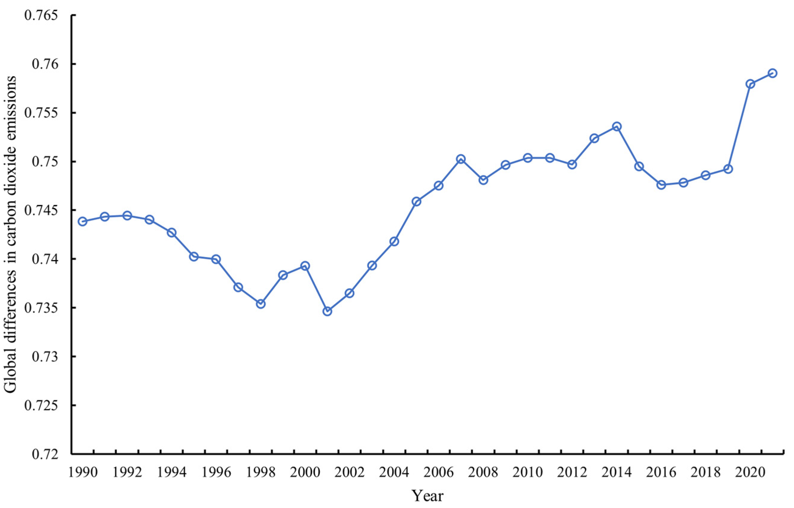
Figure 1 depicts the overall differences in CO2 emissions. According to Figure 1, it can clearly be found that the overall difference in CO2 emissions from 1990 to 2021 shows a fluctuating upward trend, which indicates that the global inequality trend in CO2 emissions is becoming more obvious during the sample study period.
The evolution trend in the Gini coefficient can be divided into four stages: the first stage was from 1990 to 2001, and the spatial differences in global CO2 emissions showed a decreasing trend. The Gini coefficient decreased from 0.7439 in 1990 to 0.7346 in 2001, with an annual average decrease of 0.1135%, indicating that the spatial difference in global CO2 emissions showed a decreasing trend from 1990 to 2001. The reason may be that after the collapse of the Soviet Union, global market mechanisms were established all over the world, which promoted the economic development of developing countries and showed a trend of the initial convergence of economic development. Therefore, the overall difference in CO2 emissions gradually decreased. Among them, the Gini coefficient from 1998 to 2001 showed a slight upward trend, mainly due to the impact of the economic crisis in Southeast Asia. The second stage was from 2001 to 2013, where the global spatial difference in carbon dioxide showed a rapidly rising trend. The Gini coefficient increased from 0.7365 in 2002 to 0.7569 in 2014, with an annual average increase of 0.2281%, indicating that the global spatial differences in CO2 emissions showed an increasing trend from 2002 to 2014. This is because China, as the largest developing country, joined the WTO after 2001. Driven by foreign trade, China’s production capacity and resource consumption capacity have been enhanced, and its global carbon emissions have increased, thus increasing the spatial differences. The third stage is from 2014 to 2019. The spatial difference in global CO2 emissions showed a rapid downward trend, and the Gini coefficient decreased from 0.7569 in 2014 to 0.7492 in 2019. The main reason is that since China proposed the Belt and Road Initiative in 2013, countries involved in the project have been promoted to optimize the green governance system and take continuous measures to reduce carbon emissions [46]. In addition, countries are paying more and more attention to the issue of climate warming and have taken action to reduce carbon emissions. The spatial differences in global carbon dioxide emissions are narrowing. The fourth stage is from 2020 to 2021. The spatial differences in global CO2 emissions are on the rise. The main reason is that the COVID-19 pandemic and Trade war has disrupted production in some countries and significantly increased the international differences in carbon dioxide emissions.
4.1.2. Intra-Regional Differences in Global Carbon Emissions
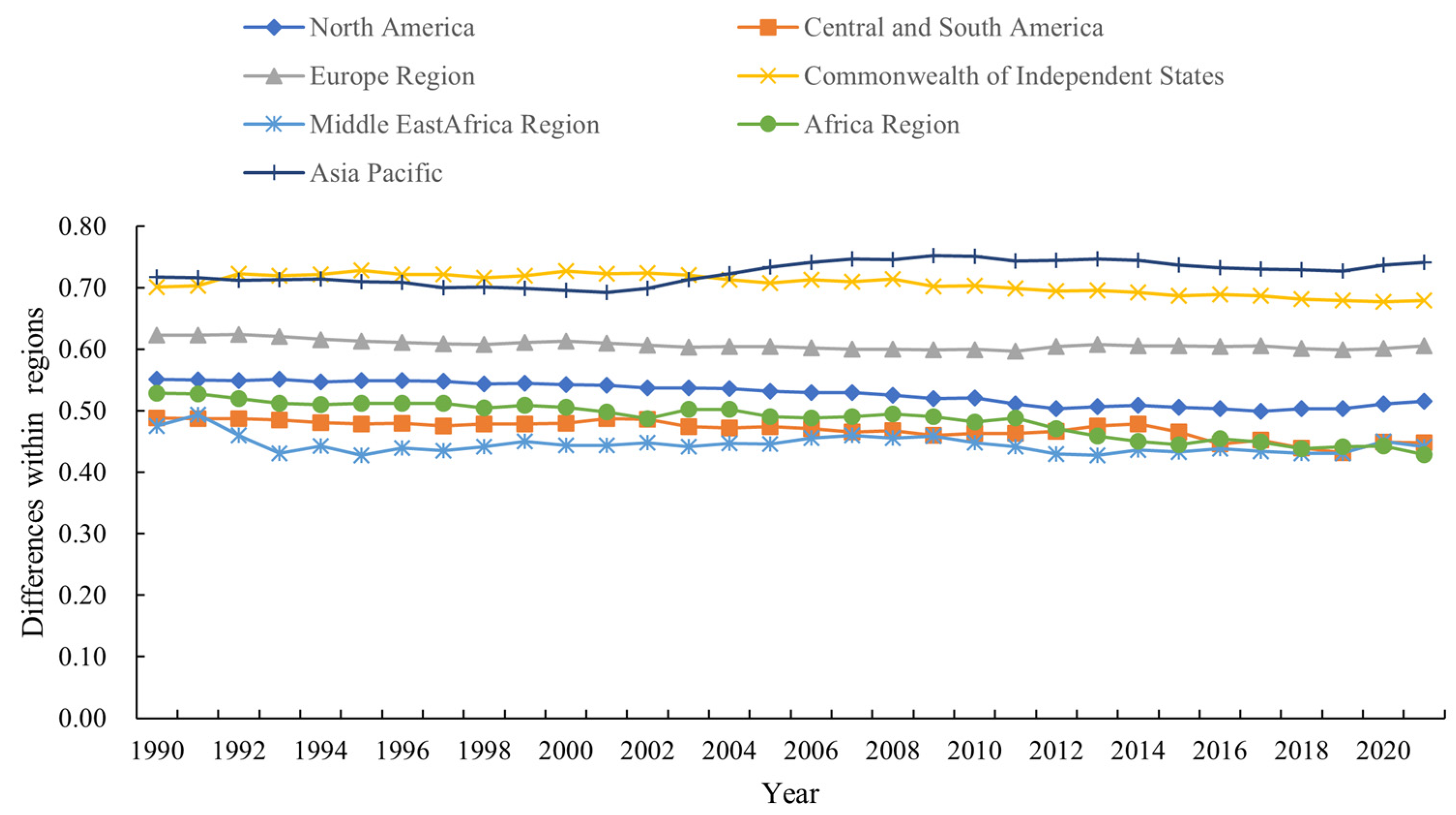
In this study, 92 countries worldwide are divided into seven regions, which are North America, Central and South America, Europe, the Commonwealth of Independent States, the Middle East, Africa, and Asia-Pacific. Figure 2 plots the intra-regional Gini coefficients for seven regions.
From Figure 2, the regional gap between the Asia-Pacific region and the Commonwealth of Independent States is much larger than that between other regions, which indicates that there is a considerable difference in CO2 emissions between the Asia-Pacific region and the Commonwealth of Independent States. This is because there is variability in the level of economic development between the Asia-Pacific region and the Commonwealth of Independent States. The Asia-Pacific region includes China, the second largest economy in the world, as well as countries with a poor level of industrialization. There are significant differences in CO2 emissions within the Asia-Pacific region. CIS countries include Russia, which has a strong industrial capacity, as well as Kazakhstan, Kyrgyzstan, and Tajikistan, which have a poor industrial capacity; thus, the CIS countries also exhibit a large difference in CO2 emissions.
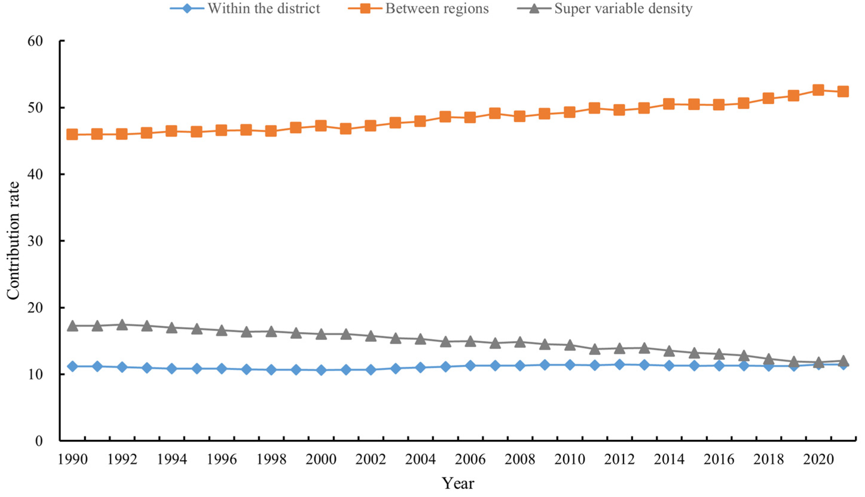
In order to determine the sources of spatial differences in global CO2 emissions, Figure 3 was derived. According to Figure 3, the contribution of regional differences in global CO2 emissions is in the order of inter-regional contribution, super-variable density, and intra-regional difference. During the sample investigation period, the difference between the interior regions contributed the most to the spatial difference in global CO2 emissions, and the contribution rate of the difference between regions remained between 45% and 55% from 1990 to 2021, and gradually increased during the sample investigation period. In addition, the contribution of the difference between regions was much higher than the difference between regions and the supervariable density. This suggests that regional disparities are the main source of global spatial differences in CO2 emissions. From 1990 to 2021, the contribution of supervariable density to the spatial difference in global CO2 emissions showed a gradually decreasing trend, whereas the contribution of intra-regional gap showed a stable trend.
4.2. Dynamic Evolution of CO2 Emission Distribution in Seven Global Regions
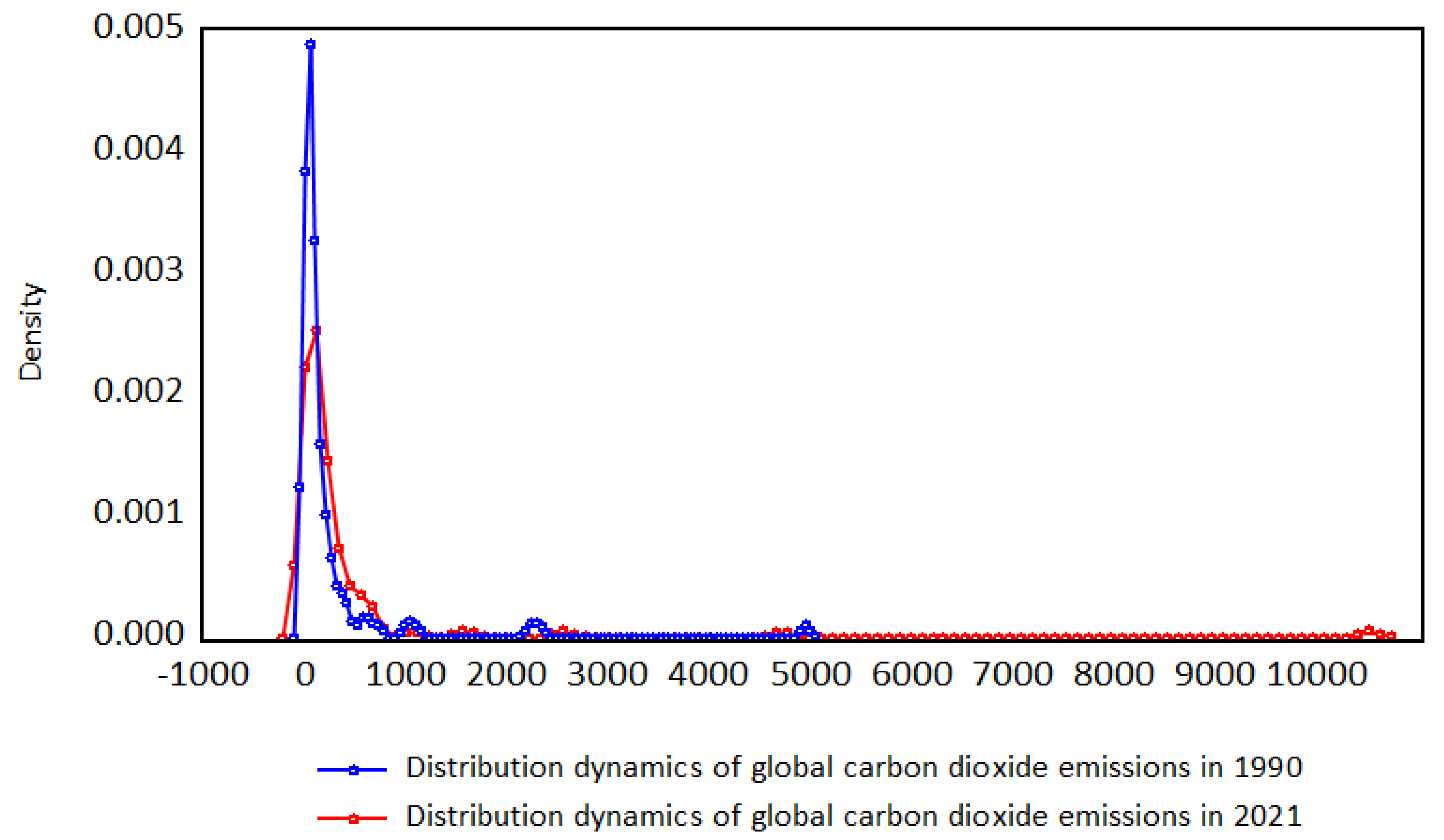
This study describes the dynamic evolution of global carbon dioxide emission distribution by drawing the kernel density map. Figure 4 depicts the dynamic evolution of global CO2 emissions distribution in 1990 and 2021.
In Figure 4, the peak value of the main peak of global CO2 emissions decreases gradually, the width of the main peak increases continuously, the distribution position of the wave crest moves to the right gradually, and there is an obvious right-trailing phenomenon; the distribution ductility is significantly expanded. This indicates that there is an obvious spatial imbalance in global CO2 emissions. Compared with 1990, the regional gap of global CO2 emissions in 2021 shows an overall widening trend. The countries with the highest CO2 emissions exhibit a large regional difference from other countries, and the multi-polar differentiation of regional differences in global CO2 emissions gradually disappears by 2021.
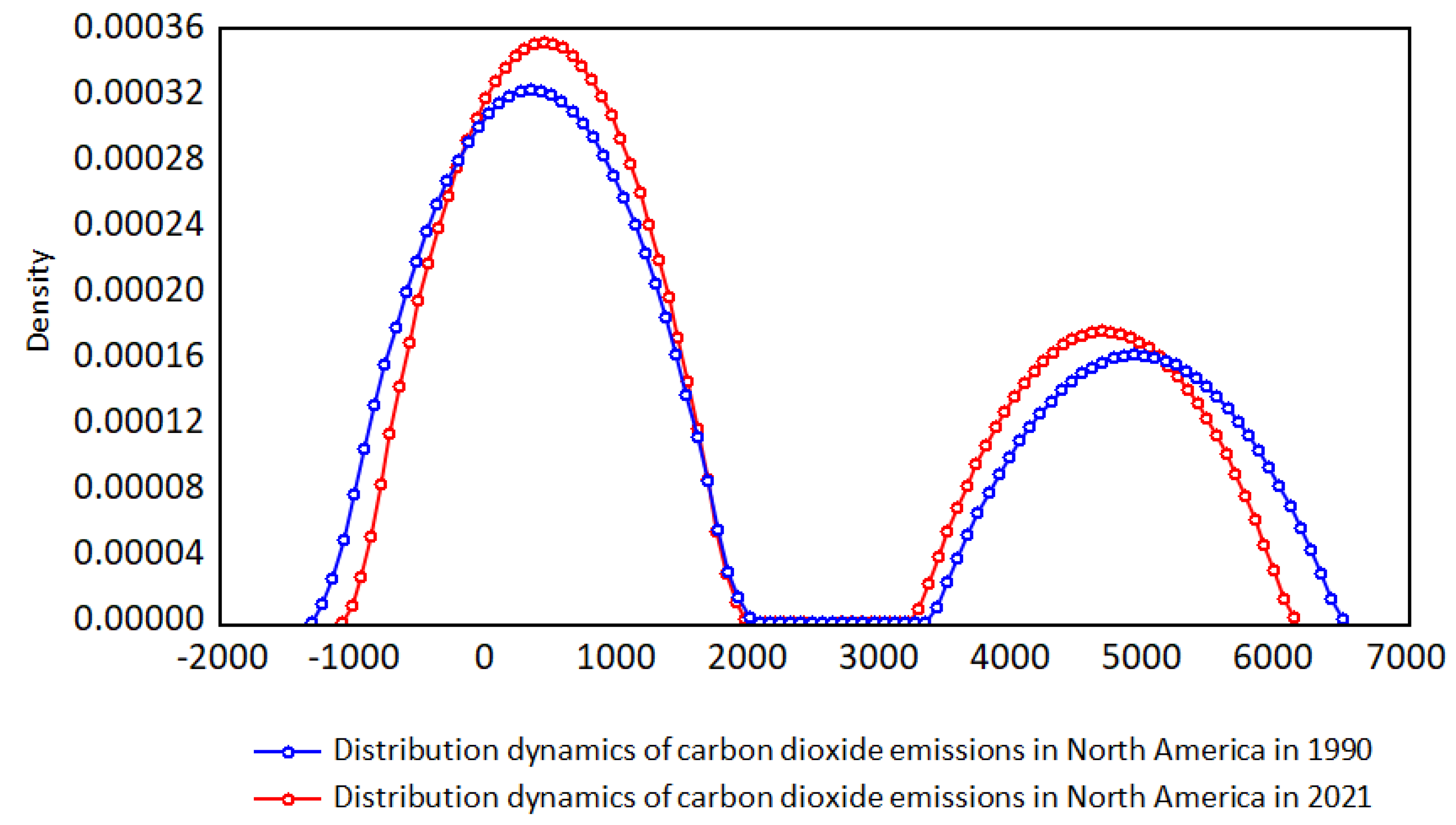
Figure 5 depicts the dynamic evolution of the distribution of global carbon dioxide emissions in North America between 1990 and 2021. According to Figure 5, compared with 1990, the nuclear density curve of CO2 emissions in North America in 2021 has an obvious leftwards trend, and there are still two peaks. The peak value increases slightly, and the ductility between the primary and secondary peaks shrinks. This shows that the carbon dioxide emission in North America presents an obvious polarization phenomenon, with little change in the regional CO2 gap. The reason is that the United States and Canada are among the world’s largest carbon emitters, with the United States being second only to China, while other countries in the region emit relatively little carbon. High-emitting countries such as the United States saw their emissions cut in 2021 due to the COVID-19 pandemic.
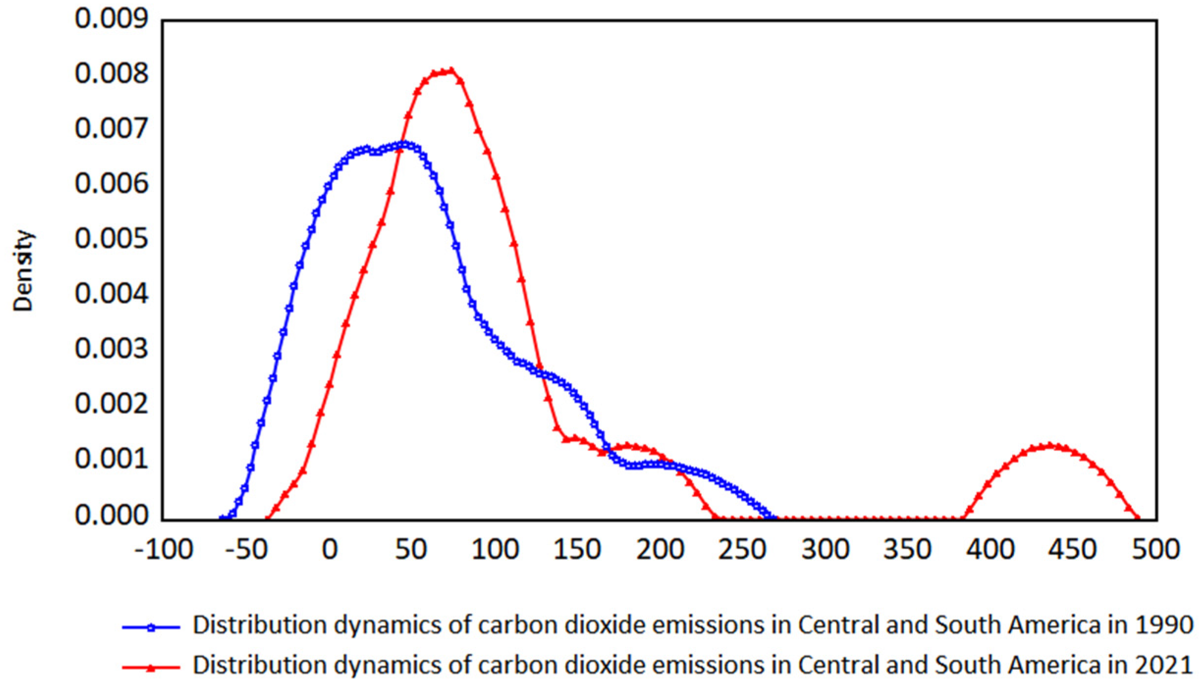
Figure 6 depicts the dynamic evolution of global CO2 emissions distribution in Central and South America between 1990 and 2021. In Figure 6, compared with 1990, the main peak of the nuclear density curve of carbon dioxide emission in Central and South America in 2021 increased, gradually shifted to the right, and the range of change expanded significantly, with two peaks obviously appearing. This shows that the regional gap of CO2 emissions in Central and South America is clearly larger, and there is a significant polarization phenomenon. The possible reason is that Brazil and Mexico are major emitters of carbon dioxide in the region, although other countries are far behind them. The destruction of the Amazon forest, known as the “world’s carbon pool”, has increased CO2 emissions. With the continuous development of the economy and society in other countries, carbon dioxide emissions have gradually increased.
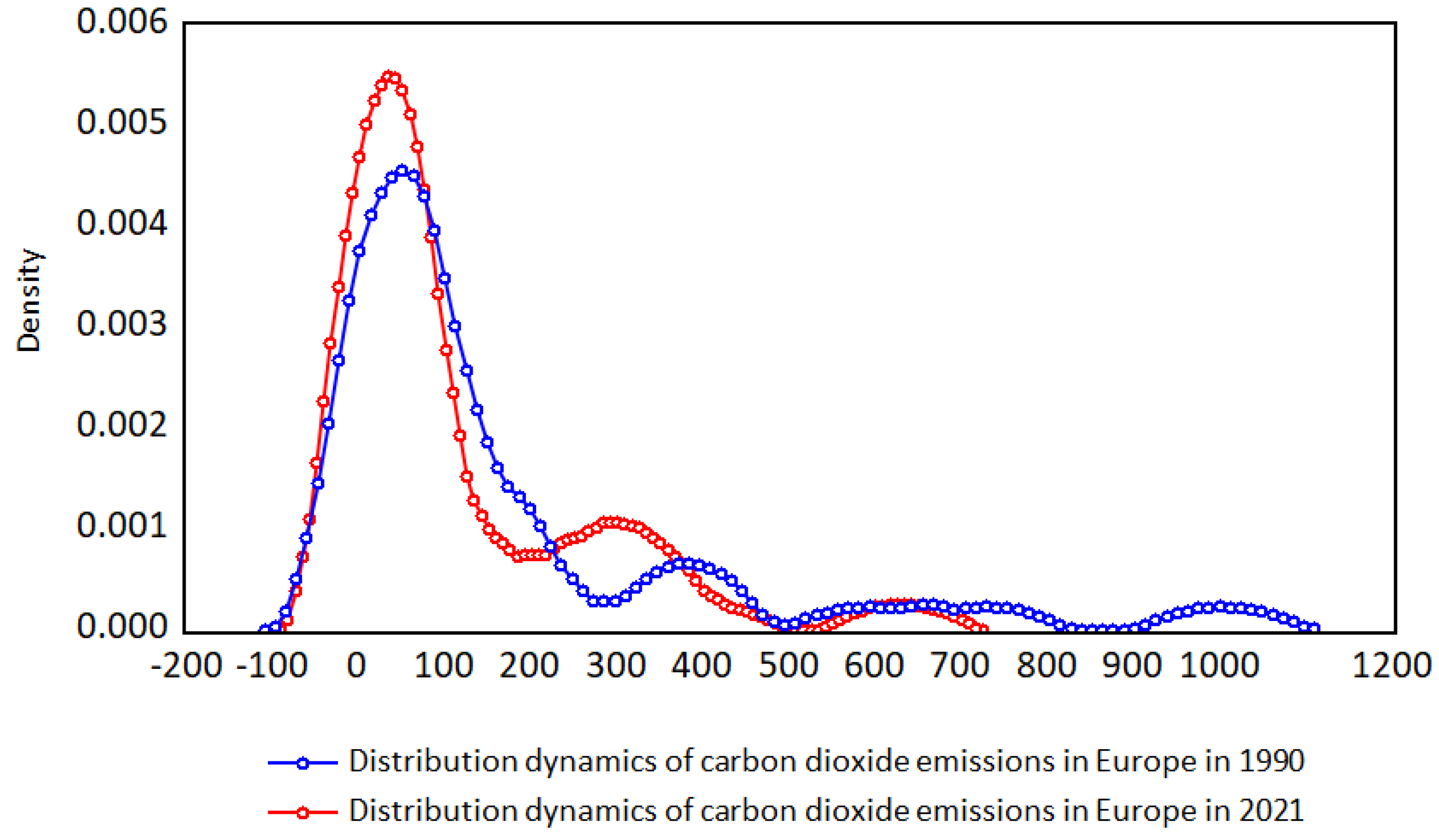
Figure 7 depicts the dynamic evolution of carbon dioxide emission distribution in Europe between 1990 and 2021. According to Figure 7, compared with 1990, the main peak of the core density curve of CO2 emissions in Europe in 2021 has increased, as has its steepness, and its sub-peak value by a large margin. Meanwhile, the number of peaks has decreased from four to three. The core density curve has shifted slightly to the left, but the moving trend is not obvious, the change range has narrowed, and the ductility has decreased. This shows that the regional gap of CO2 emissions in Europe has narrowed, and the multi-polarization phenomenon has eased, but it is still facing a triple-polarization phenomenon. The reason may be that a series of carbon reduction agreements formulated by the EU has played a key role. In particular, the rapid development of new energy vehicles has reduced the use of traditional energy sources such as oil and effectively reduced carbon dioxide emissions. The phenomenon of multi-level differentiation indicates that the major carbon emitters in Europe are still Germany, the United Kingdom, France, and other traditional industrial powers.
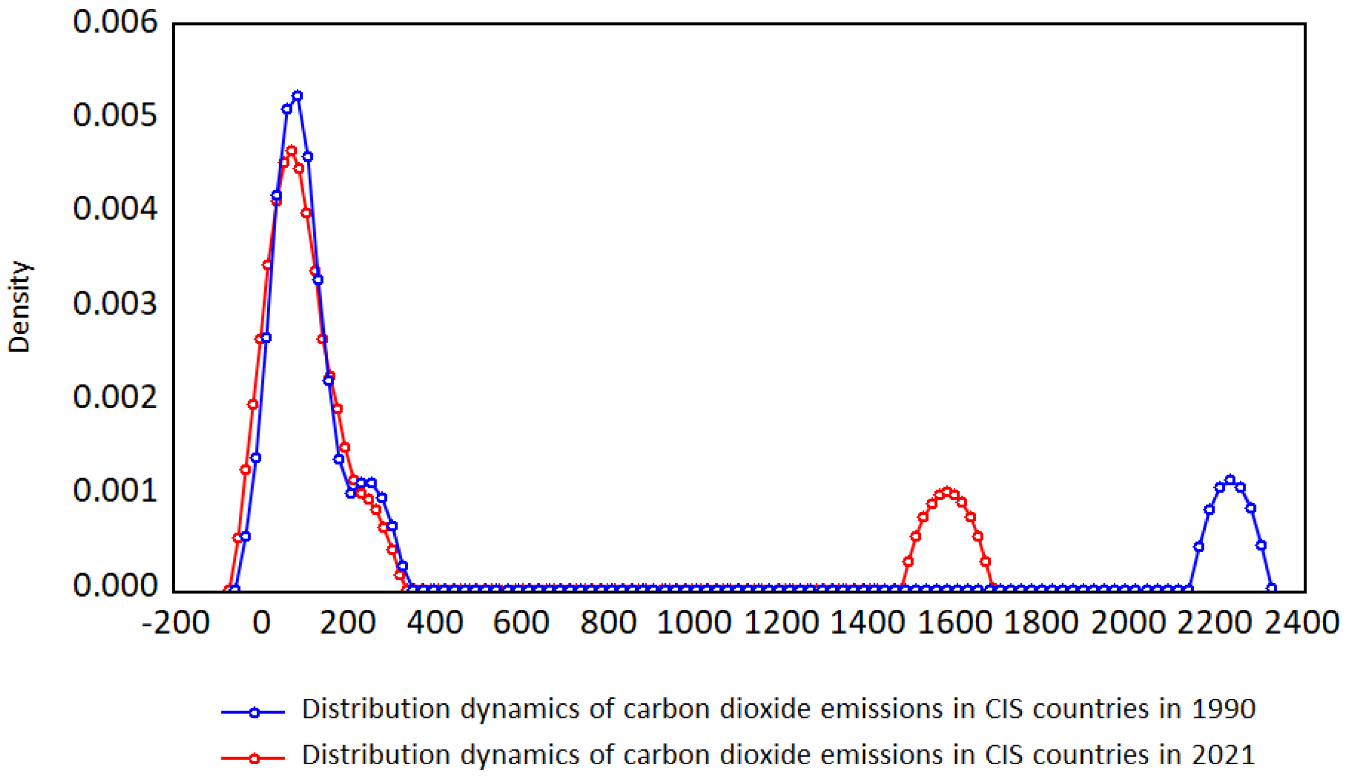
Figure 8 depicts the dynamic evolution of global CO2 emissions distribution in the CIS countries between 1990 and 2021. According to Figure 8, compared with 1990, in 2021, the nuclear density curve of carbon dioxide emission in CIS countries moved slightly on the whole, and both the main peak and sub-peak values decreased. The sub-peak shifted to the left significantly, the range of change narrowed, and the right-trailing phenomenon eased somewhat. This indicates that the regional disparity of CO2 emissions in CIS countries is not obvious and still presents a two-level differentiation trend. The reason is that Russia, as the largest industrial power in the region, emits a lot of carbon dioxide, whereas countries such as Kazakhstan and Kyrgyzstan are underdeveloped in heavy industry and emit relatively little carbon.
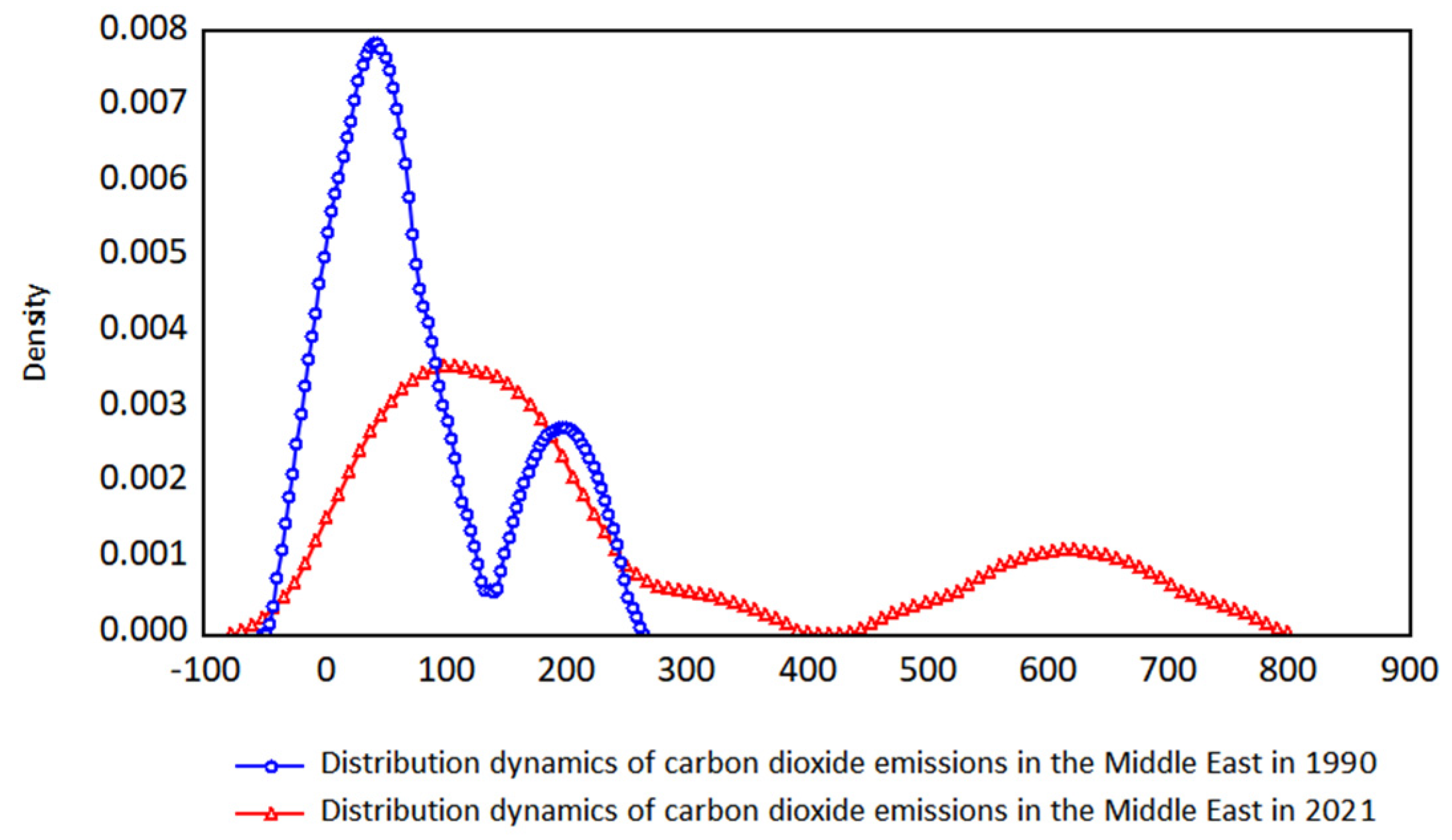
Figure 9 depicts the dynamic evolution of global CO2 emissions distribution in the Middle East between 1990 and 2021. According to Figure 9, carbon dioxide emissions in the Middle East as a whole increased in 2018 compared with 1990. The main peak and sub-peak values of the nuclear density curve of CO2 emissions in the Middle East in 2021 decreased significantly, the width increased significantly, and the steepness of the bimodal peaks decreased significantly. However, there was still an obvious bimodal pattern, with the right-trailing phenomenon increasing significantly, the ductility widening, and the range of variation expanding significantly. This shows that regional differences in CO2 emissions in the Middle East have widened significantly and are still polarized. The reason is that the countries in this region are mainly oil-producing countries, and their carbon emissions are mainly concentrated in Iran, Saudi Arabia and Turkey. Other countries are affected by wars and internal political changes; thus, they have slower economic growth and lower carbon dioxide emissions.
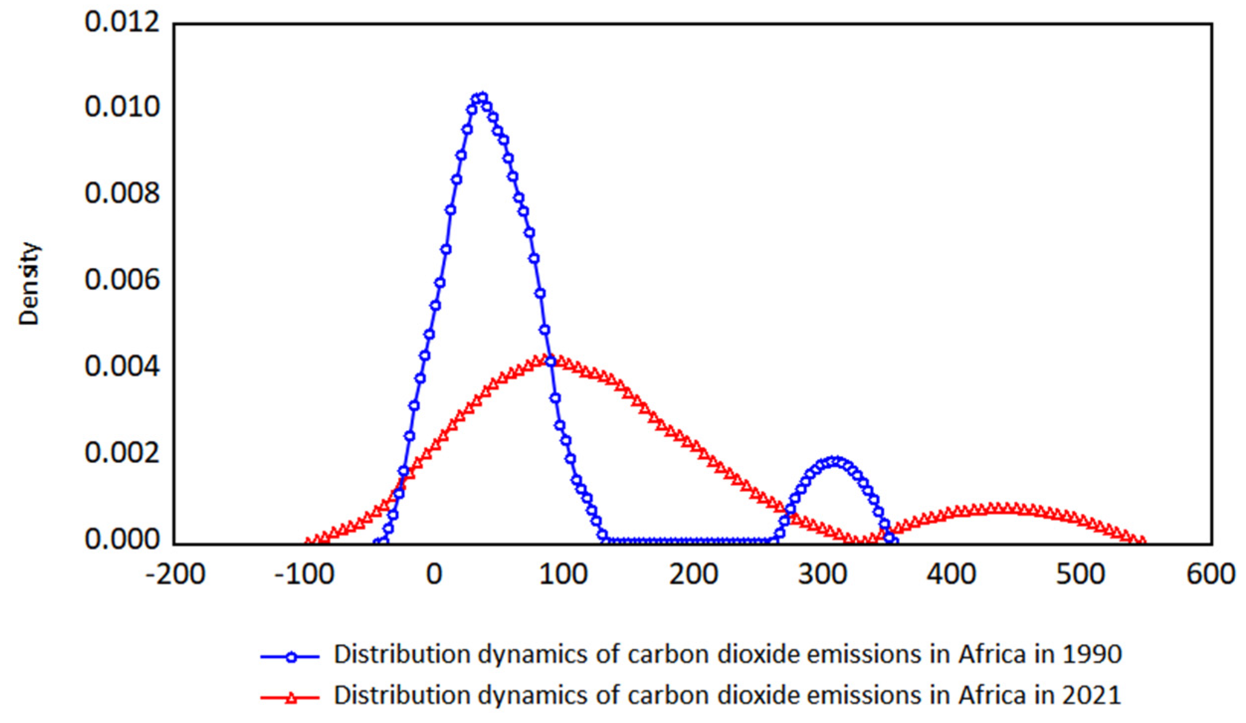
Figure 10 depicts the dynamic evolution of global CO2 emissions in Africa between 1990 and 2021. According to Figure 10, compared with 1990, both the main peak and sub-peak of the nuclear density curve of CO2 emissions in Africa in 2021 significantly decreased, the steepness of the two peaks significantly decreased, the bimodal pattern remained, the ductility widened, and the range of variation significantly expanded. This shows that the regional differences in CO2 emissions in Africa are obviously widening, and the phenomenon of polarization still exists. The likely reason is that economically developed South Africa is the “backbone” of the region’s CO2 emissions, while other regions, especially sub-Saharan Africa, have long been in deep poverty and emit less carbon dioxide.
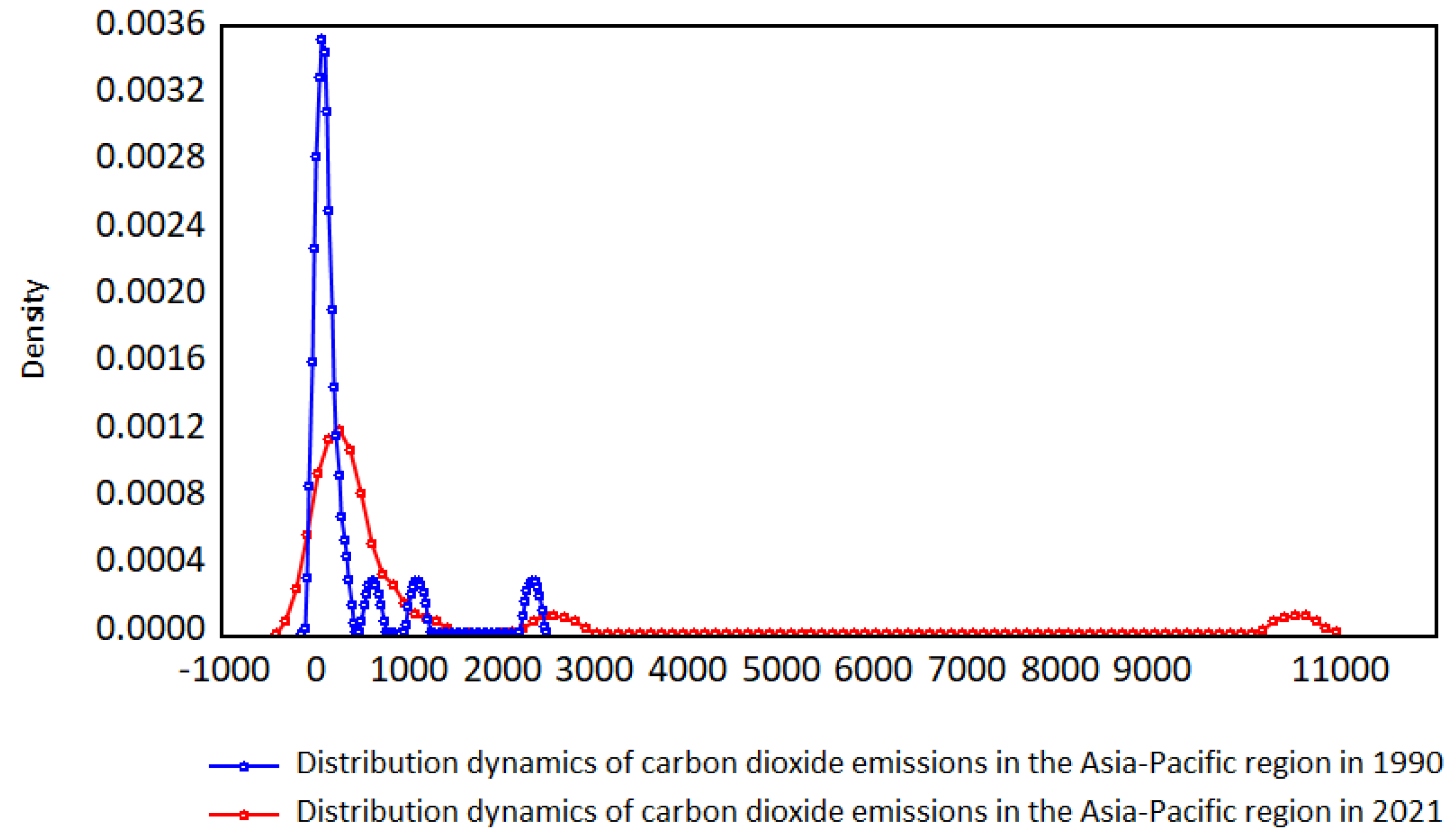
Figure 11 depicts the dynamic evolution of the global carbon dioxide emission distribution in the Asia-Pacific region between 1990 and 2021. According to Figure 11, compared with 1990, the main peak of the nuclear density curve of CO2 emissions in the Asia-Pacific region in 2021 decreased significantly, the steepness decreased, the double-peak pattern remained, the right-trailing phenomenon was obvious, the ductility widened, the range of variation expanded significantly, and the number of peaks decreased from four to three. It shows that the regional gap of CO2 emissions in the Asia-Pacific region is clearly larger, and the multi-level differentiation phenomenon persists. The reason is that the region is home not only to China, which is the largest emitter of carbon dioxide, but also to India, Indonesia, Japan, South Korea and other major carbon emitters. In particular, the global trade war against China in recent years has led to the relocation of manufacturing to India, Vietnam and other countries, resulting in a growing number of countries with high carbon emissions. It is also home to slow developing countries such as North Korea and Mongolia. As a result, the Asia-Pacific region has become the region with the highest CO2 production and the biggest differences in the world, and has become the “main front” of global carbon pollution reductions. 4.3. Markov chain analysis of global CO2 emissions.
Before analyzing the Markov chain, the CO2 emissions of 92 countries were ranked from low to high, and the entire sample was divided into four levels, in which CO2 emissions in the range of 0~25% are low level, 25~50% are medium-low level, 50~75% are medium-high level and 75~100% are high level. On this basis, the Markov transfer probability matrix of global CO2 emissions from 1992 to 2021 was measured when the lag period was years and years; the results are shown in Table 1. When the lag time was , the transfer probability value on the main diagonal of global CO2 emissions was much greater than that of other positions, which indicates that the dynamic distribution law of global CO2 emissions is stable, the inter-group mobility of CO2 emissions is low, the relative position of global CO2 emissions is stable, and different groups all transfer to themselves with a greater probability. This indicates that global CO2 emissions are still at a high level in the short term, and achieving global carbon peaking and carbon neutrality will be a long-term process. The probability of the transfer from the high-carbon emission group to the medium-low carbon emission group and the low-carbon emission group is 0, and the probability of the transfer from the medium-low carbon emission group and the low-carbon emission group to the high-carbon emission group is 0, which indicates that there is no possibility of the global carbon dioxide emission transferring from the low-carbon emission group to the high-carbon emission group in the short term, and there is no possibility of the transfer from the high-carbon emission group to the low-carbon emission group. With the increase in lag period, the probability value on the main diagonal showed a gradual decline trend.
From lag period 1 to lag period 5, the probability of transfer from the high-carbon emission group to the high-carbon emission group was 0.9590→0.94293→0.9203→0.8966→0.8746→0.8546, indicating that with the extension of the time span, the possibility of the inter-group transfer of global CO2 emissions is gradually reduced, which indicates that with the continuous progress in green innovation technology and international cooperation on climate change, CO2 emissions from the high-carbon emission group will gradually be transferred to the low-carbon emission group. From lag period 1 to lag period 5, the probability of the high-carbon emission group transferring to the medium-high carbon emission group is 0.0410→0.0571→0.0782→0.1019→0.1238→0.1438, which indicates that with the extension of time span, the possibility of global carbon dioxide emission transferring from the high-carbon emission group to the medium-high carbon emission group will increase gradually. This suggests a gradual decline in global CO2 emissions over time.
4.3. Analysis of Convergence Characteristics of Global CO2 Emissions
4.3.1. σ Convergence Analysis of Global CO2 Emissions
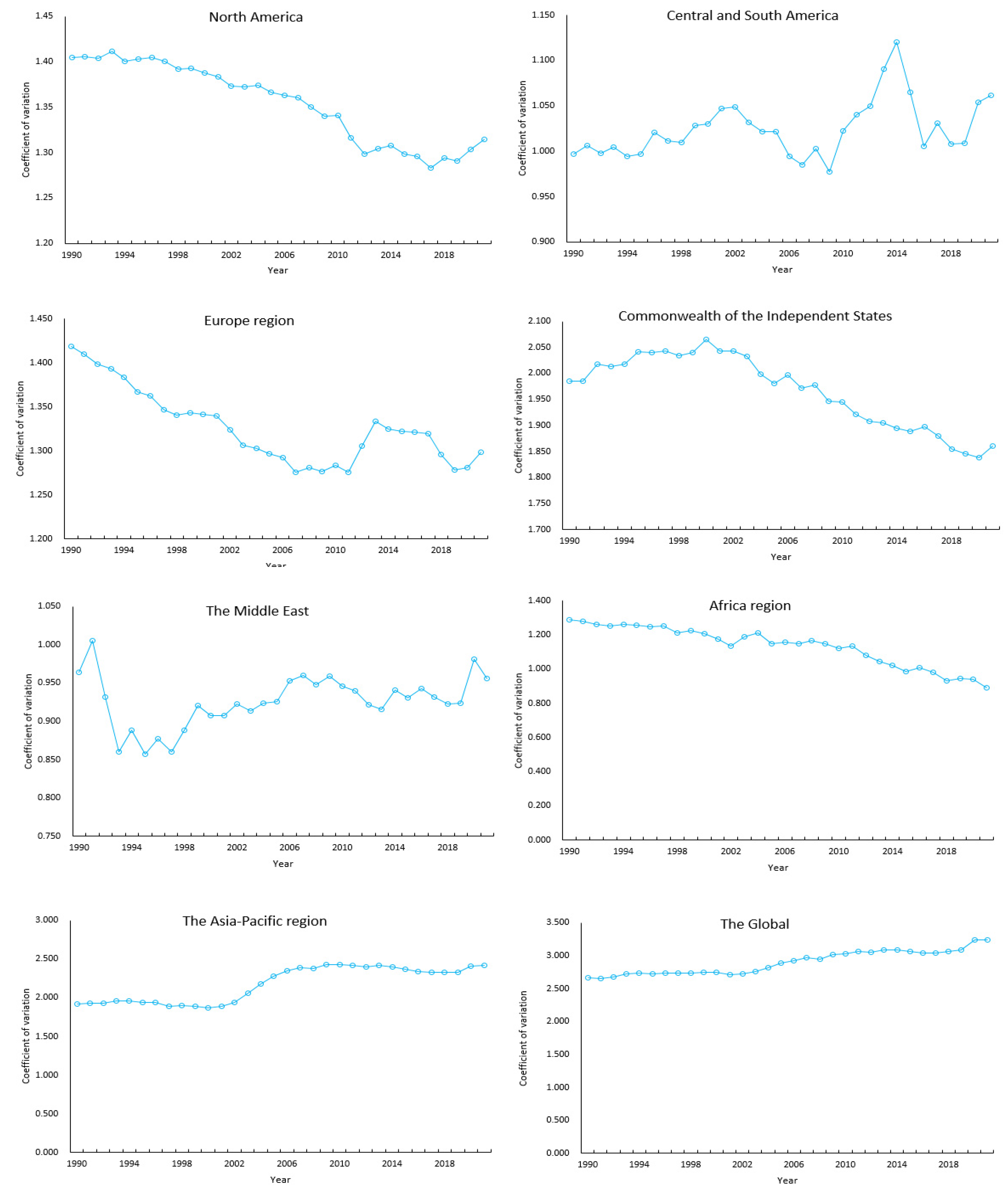
In order to reveal the convergence characteristics of global CO2 emissions, this study measured the coefficient of variation in the global, North America, Central and South America, Europe, the Commonwealth of Independent States, the Middle East, Africa, and the Asia-Pacific regions. Figure 12 shows the evolution trend in the covariance of CO2 emissions globally and in seven regions of the world from 1990 to 2021.
The evolution trend of global covariance showed a gradually increasing trend during the sample study period, which increased from 2.660 in 1990 to 3.244 in 2021, with an annual growth rate of 1.88%. Among them, it was the lowest in 2002. Later, with the increase in global economic development and the difference in fossil energy consumption, the spatial difference in carbon dioxide emissions further increased. This indicates that there was no σ convergence in global CO2 emissions from 1990 to 2021. From the evolution trend in the variation coefficients of the seven regions in the world, the variation coefficients of North America, Europe, the Commonwealth of Independent States and Africa showed a gradual downward trend during the sample study period, with average annual decline rates of 0.29%, 0.39%, 0.4% and 1.28%, respectively, indicating the convergence characteristics of CO2 emissions in these regions. The coefficients of variation in Central and South America and Asia-Pacific showed a gradual upward trend from 1990 to 2021, with average annual growth rates of 0.21% and 1.61%, respectively. This indicates that CO2 emissions in Central and South America and the Asia-Pacific have divergent characteristics, but not σ convergence. The coefficient of variation in CO2 emissions in the Middle East showed a stable trend. During the study period, the Middle East region had suffered from long-term war and economic stagnation; thus, there was no obvious convergence and divergence of CO2 emissions.
4.3.2. Absolute β Convergence Analysis of Global CO2 Emissions
Table 2 shows the absolute β convergence of CO2 emissions in the whole region. The results show that no matter the fixed effect or random effect, the convergence coefficient is always positive and passes the significance test of 1%, which indicates that with the increase in global carbon dioxide emissions, the growth rate of global carbon dioxide emissions is gradually decreasing. The regression results of the two-way fixed effect model show that the influence coefficient of global carbon dioxide emissions on the growth rate of carbon dioxide emissions is −0.0608, which also passes the significance level test of 1%, indicating the absolute β convergence of global carbon dioxide emissions. This is due to the concerted efforts of the international community to reach a consensus on carbon reduction in the context of global warming. In particular, Chinese society has actively participated in carbon reduction efforts, actively following the global trend of green and low-carbon development, and has actively and scientifically laid out carbon peaking targets, making important contributions to global carbon reduction.
5. Conclusions
Faced with the reality of climate warming, how to reduce carbon emissions has become a hot issue that increasingly concerns the governments of all countries [47,48]. Understanding the differences and sources of global carbon dioxide emissions and grasping the trends in global carbon dioxide emissions is of great significance for the differentiated and targeted development of national emission reduction strategies. Compared with traditional methods, the Dagum Gini coefficient can effectively solve the source problem of regional differences [13]. Therefore, this study first -adopted this method to measure the spatial differences of CO2 emissions in seven regions of the world, and -revealed the sources of differences. Then, the dynamic evolution law of global CO2 emissions and seven regions was analyzed, and finally, the convergence characteristics of global CO2 emissions were demonstrated. The results are -presented subsequently.
From the perspective of overall differences, the overall differences in global carbon dioxide emissions during the study period showed a gradually increasing trend. This indicates that the trend in global inequality in carbon dioxide becomes more obvious during the sample period. This is consistent with the conclusion of Bolea et al. [2]. In particular, the evolution of global carbon dioxide inequality shows a downward trend, then an upward trend, and then a downward trend. This can be explained from two aspects: on the one hand, in the wave of international industrial transfer, high-income countries will transfer energy-intensive and high-emission industries to low-income countries, resulting in the rapid growth of emissions of many low—and middle-income countries with high carbon emissions in the first place [49]. On the other hand, many high-income countries such as the United States have reached peak carbon dioxide emissions, and with the application of new technologies and the upgrading of industrial structures, carbon emissions are decreasing year by year [50]. The spatial differences in regional CO2 emissions are profound in Asia-Pacific, CIS countries, Europe, North America, Africa, Central and South America, and the Middle East. From the perspective of distribution dynamics, the peak value of the main peak of global carbon dioxide emission decreased gradually, the width of the main peak increased continuously, and the distribution position of the wave crest gradually moved to the right, with an obvious right-trailing phenomenon, and the distribution ductility is significantly expanded. This indicates that there is an obvious spatial disequilibrium of global CO2 emissions. From the perspective of evolution law, the transfer probability value on the main diagonal of the transfer probability matrix is much greater than that of other positions, indicating that the dynamic distribution law of global CO2 emissions is stable, the mobility of CO2 emissions between groups is low, the relative position of global CO2 emissions is stable, and different groups transfer to themselves with a greater probability. From the convergence characteristics, there is no obvious σ convergence in global carbon dioxide emissions, but there is absolute β convergence.
Combined with the research results, the policy recommendations are drawn:
- It is necessary to fully understand the spatial imbalance of global CO2 emissions and to formulate carbon peaking and carbon neutrality road maps according to different stages of national economic development. On the one hand, for developing countries, it is still an important task to achieve economic catch-up and improve the living standards of their citizens, and at the same time, it is necessary to take overall consideration. The relationship between development and environmental protection should be handled carefully to achieve green development. On the other hand, developed countries should take the initiative to shoulder the historical responsibility of carbon dioxide emission and promote the “net zero emission” of global carbon dioxide.
- Regional differences in global CO2 emissions are the main source of overall differences. Therefore, regional differences in CO2 emissions should be narrowed to achieve the balanced development of global carbon dioxide emission reductions. The transfer of carbon reduction technologies should be gradually realized from developed countries to developing countries, and help developing countries effectively control carbon dioxide. Market means should be adopted to optimize the allocation of carbon emission trading rights between developing and developed countries, so as to achieve carbon emission reduction.
- Regions with high carbon emissions should pay attention to intra-regional carbon emission reduction work, make comprehensive use of both market and government resource allocation methods, find a good combination of environmental regulations, and use command, market and public environmental regulations to form a carbon reduction force.
- Countries should carry out cooperation and exchanges on the global governance of CO2 emissions, and gradually realize a carbon emission reduction system featuring technology, experience and data sharing. Under the guidance of the China-proposed community of a shared future for mankind, we should build a global community with the goal of reducing pollution and carbon.
The findings of this study contribute to developing an understanding of the overall differential characteristics of carbon dioxide emissions around the world and within the seven regions studied here, and facilitate the further definition of countries’ emission reduction responsibilities. However, limited by data acquisition, only macro data between countries were analyzed, without considering carbon emissions at the enterprise level. In the future, with the development of Python big data crawler technology, the availability of enterprise data will be enhanced, and we will continue to use enterprise data for research. In this way, we can develop a more detailed understanding of the differences in carbon emissions between different countries, different industries and different industries.
Author Contributions
Conceptualization, X.G.; methodology, L.H.; software, L.H.; Writing—original draft, L.H.; Writing—review and editing, J.L. and X.G. All authors have read and agreed to the published version of the manuscript.
Funding
This study was funded by The National Social Science Foundation of China (20CJL008) and Special Fund of Social Science Layout Study in Shandong Province (19CDCJ08).
Informed Consent Statement
Informed consent was obtained from all subjects involved in the study.
Data Availability Statement
The data used to support the findings of this study are included within the article.
Acknowledgments
The authors wish to thank the Editors of this issue and all reviewers for their useful insights and constructive comments on previous versions of this study.
Conflicts of Interest
The authors declare no conflict of interest.
References
- Duro, J.A.; Teixidó-Figueras, J.; Padilla, E. Empirics of the international inequality in emissions intensity: Explanatory factors according to complementary decomposition Methodologies. Environ. Resour. Econ. 2016, 63, 57–77. [Google Scholar] [CrossRef]
- Bolea, L.; Duarte, R.; Sanchez-Choliz, J. Exploring carbon emissions and international inequality in a globalized world: A multiregional-multispectral perspective–Science Direct. Resour. Conserv. Recycl. 2020, 152, 104516. [Google Scholar] [CrossRef]
- World Health Organization. Available online: https://www.who.int/news-room/fact-sheets/detail/climate-change-and-health (accessed on 2 February 2023).
- Chen, H.; Chen, W.; He, J. Pathway to meet carbon emission peak target and air quality standard for China. Chin. J. Popul. Resour. 2020, 30, 12–18. [Google Scholar]
- Jiang, M.; An, H.; Gao, X. Adjusting the global industrial structure for minimizing global carbon emissions: A network-based multi-objective optimization approach. Sci. Total Environ. 2022, 829, 154653. [Google Scholar] [CrossRef]
- Wang, M.; Feng, C. Decoupling economic growth from carbon dioxide emissions in China’s metal industrial sectors: A technological and efficiency perspective. Sci. Total Environ. 2019, 691, 1173–1181. [Google Scholar] [CrossRef] [PubMed]
- Xu, W.; Zhou, J.; Liu, C. The impact of digital economy on urban carbon emissions: Based on the analysis of spatial effects. Geogr. Res. 2022, 41, 111–129. [Google Scholar]
- Lin, L.; Yang, Q. Does green infrastructure investment reduce carbon emissions? Mod. Econ. Res. 2022, 12, 29–37. [Google Scholar]
- Wang, X.; Cheng, Y. Research on the influencing mechanism of urbanization on carbon emission efficiency—Based on an empirical study of 118 countries. World Reg. Stud. 2020, 29, 503–511. [Google Scholar]
- You, Z.; Peng, Z.; Li, P. Research on the impact of green finance development on regional carbon emission: Take green credit green industrial investment and green bonds for example. Financ. Theory Pract. 2022, 2, 69–77. [Google Scholar]
- Wang, Z.; Fan, J. The characteristics and prospect of influencing factors of energy-related carbon emissions: Based on literature review. Geogr. Res. 2022, 41, 2587–2599. [Google Scholar]
- Li, G.; Li, Z. Regional differences and influencing factors of carbon dioxide emissions in China. Chin. J. Popul. Resour. 2010, 20, 22–27. [Google Scholar]
- Liu, H.; Zhao, H. Analysis of regional differences in carbon dioxide emission intensity in China. Stat. Res. 2012, 29, 46–50. [Google Scholar]
- Dechezleprêtre, A.; Nachtigall, D.; Venmans, F. The Joint Impact of the European Union Emissions Trading System on Carbon Emissions and Economic Performance. OECD Economics Department & Environment Directorate Bruegel, 6 December 2018. Available online: https://www.oecd.org/economy/greeneco/can-we-reduce-emissions-without-hurting-jobs/joint-impact-of-the-EU-ETS-on-carbon-emissions-and-economic-performance-OECD-december-2018.pdf (accessed on 14 March 2023).
- Alaganthiran, R.J.; Anaba, M.I. The effects of economic growth on carbon dioxide emissions in selected Sub-Saharan African (SSA) countries. Heliyon 2022, 8, 11193. [Google Scholar] [CrossRef] [PubMed]
- Heil, M.T.; Wodon, Q.T. Inequality in CO2 emissions between poor and rich countries. J. Environ. Dev. 1997, 6, 426–452. [Google Scholar] [CrossRef]
- Duro, J.A.; Padilla, E. International inequalities in per capita CO2 emissions: A decomposition methodology by Kaya factors. Energy Econ. 2006, 28, 170–187. [Google Scholar] [CrossRef]
- Padilla, E.; Serrano, A. Inequality in CO2 Emissions across Countries and Its Relationship with Income Inequality: A Distributive Approach. Energy Policy 2006, 34, 1762–1772. [Google Scholar] [CrossRef] [Green Version]
- Brahmasrene, T.; Lee, J.W. Assessing the dynamic impact of tourism, industrialization, urbanization, and globalization on growth and environment in Southeast Asia. Int. J. Sustain. Dev. World Ecol. 2017, 24, 362–371. [Google Scholar] [CrossRef]
- Huang, H.; Qiao, X.; Zhang, J. Analysison spatial-temporal evolution of carbon Emission of tourist industry in Vanatze River economic zone. Guizhou Soc. Sci. 2019, 350, 143–152. [Google Scholar]
- Zhang, L.; Li, D.; Zhou, D. Dynamic changes and regional differences in carbon dioxide emission performance of China’s logistics industry: An empirical analysis based on provincial panel data. Systems Eng. 2013, 4, 95–102. [Google Scholar]
- Wang, X.; Li, B.; Lv, C.; Guan, Z.; Cai, B.; Lei, Y.; Yan, G. China’s iron and steel industry carbon emissions peak pathways. Res. Environ. Sci. 2022, 35, 339–346. [Google Scholar]
- Jin, S.; Lin, Y.; Niu, K. Driving green transformation of agriculture with low carbon: Characteristics of agricultural carbon emissions and its emission reduction path in China. Reform 2021, 327, 29–37. [Google Scholar]
- Zhang, C.; Xie, X.; Cao, B. Analysis on the difference of carbon dioxide emission and its influencing factors among different Industries in China--Empirical analysis based on the improved STIRPAT Model. Ecol. Econ. 2012, 9, 3–116. [Google Scholar]
- Lin, X.; Bian, Y.; Wang, D. Spatiotemporal evolution characteristics and influencing factors of industrial carbon emission efficiency in Beijing-Tianjin-Hebei region. Econ. Geogr. 2021, 41, 187–195. [Google Scholar]
- Tan, D.; Huang, X. Correlation analysis and Comparison between economic development and carbon emission in East, Middle and west regions of China. Chin. J. Popul. Resour. 2008, 18, 54–57. [Google Scholar]
- Li, X.; Wang, A.; Yu, W. Global CO2 emission trend analysis based on energy demand theory. Acta Geosci. Sin. 2010, 31, 741–748. [Google Scholar]
- Davis, S.J.; Caldeira, K.; Matthews, H.D. Future CO2 emissions and climate change from existing energy infrastructure. Science 2010, 329, 1330–1333. [Google Scholar] [CrossRef] [Green Version]
- Yang, Q.; Liu, H. Regional differences and convergence of carbon intensity distribution in China: An empirical study based on provincial data from 1995 to 2009. Contemp. Financ. Econ. 2012, 2, 89–100. [Google Scholar]
- Clarke-Sather, A.; Qu, J.; Wang, Q.; Zeng, J.; Li, Y. Carbon inequality at the sub-national scale: A case study of provincial-level inequality in CO2 emissions in China 1997–2007. Energy Policy 2011, 39, 5420–5428. [Google Scholar] [CrossRef]
- Han, M.; Liu, W.; Xie, Y. Regional disparity and decoupling evolution of China’s carbon emissions by province. Resour. Sci. 2021, 43, 710–721. [Google Scholar]
- Wang, R.; Zhang, H.; Qiang, W.; Li, F.; Peng, j. Spatial characteristics and influencing factors of carbon emissions in county-level cities of China based on urbanization. Prog. Geogr. 2021, 40, 1999–2010. [Google Scholar] [CrossRef]
- Niu, Y.; Zhao, X.; Hu, Y. Spatial variation of carbon emissions from county land use in Chang-Zhu-Tan area based on NPP-VIIRS night light. Acta Sci. Circumstantiae 2021, 41, 3847–3856. [Google Scholar]
- Li, X.; Lin, B. Global convergence in per capita CO2 emissions. Renew. Sustain. Energy Rev. 2013, 24, 357–363. [Google Scholar] [CrossRef]
- Westerlund, J.; Basher, S.A. Testing for convergence in carbon dioxide emissions using a century of panel data. Environ. Resour. Econ. 2008, 40, 109–120. [Google Scholar] [CrossRef]
- Romero-Avila, D. Convergence in carbon dioxide emissions among industrialized countries revisited. Energy Econ. 2008, 30, 2265–2282. [Google Scholar] [CrossRef]
- Gao, M.; Song, H. Dynamic changes and spatial agglomeration analysis of the Chinese agricultural carbon emissions performance. Econ. Geogr. 2015, 35, 142–148+185. [Google Scholar]
- Sefa, A.C.; John, L.; Kris, I. Conditional convergence in per capita carbon emissions since 1900. Appl. Energy 2018, 228, 916–927. [Google Scholar]
- El-Montasser, G.; Inglesi-Lotz, R.; Gupta, R. Convergence of greenhouse gas emissions among G7 countries. Appl. Econ. 2015, 47, 6543–6552. [Google Scholar] [CrossRef] [Green Version]
- Aldy, J.E. Per capita carbon dioxide emissions: Convergence or divergence? Environ. Resour. Econ. 2006, 33, 533–555. [Google Scholar] [CrossRef] [Green Version]
- Zhang, Z.Q.; Zhang, T.; Feng, D.F. Study on regional differences dynamic evolution and convergence of carbon emission intensity in China. J. Quant. Technol. Econ. 2022, 39, 67–87. [Google Scholar]
- Liu, H.; Du, G. Regional disparity and stochastic convergence test of China’s economic development: Based on DMSP/OLS night light data from 2000 to 2013. J. Quant. Technol. Econ. 2017, 10, 43–59. [Google Scholar]
- Liu, H.; He, L.; Yang, Q. Spatial disequilibrium and dynamic evolution of population aging in China: 1989–2011. Popul. Res. 2014, 2, 71–82. [Google Scholar]
- Liu, C.; Wang, H.; Wei, X. Research on regional difference decomposition and convergence of internet finance development in eight urban agglomerations of China. J. Quant. Technol. Econ. 2017, 8, 4–21. [Google Scholar]
- Liu, C.; Yin, X.; Wang, L. Regional differences and dynamic evolution of distribution of digital economy in China. Forum Sci. Technol. China 2020, 287, 97–109. [Google Scholar]
- Zhou, Y. Green governance in global value chains: Status adjustment and relationship remodeling between North and South Countries. Dipl. Rev. (J. China Foreign Aff. Univ.) 2019, 36, 49–80. [Google Scholar]
- Wiedmann, T. A review of recent multi-region input–output models used for consumption-based emission and resource accounting. Ecol. Econ. 2009, 69, 211–222. [Google Scholar] [CrossRef]
- Kennedy, C.; Steinberger, J.; Gasson, B.; Hansen, Y.; Hillman, T.; Havránek, M.; Pataki, D.; Phdungsilp, A.; Ramaswami, A.; Mendez, G.V. Methodology for inventorying greenhouse gas emissions from global cities. Energy Policy 2010, 38, 4828–4837. [Google Scholar] [CrossRef]
- Nan, S.; Huo, Y.; You, W.; Guo, Y. Globalization spatial spillover effects and carbon emissions: What is the role of economic complexity? Energy Econ. 2022, 112, 106184. [Google Scholar] [CrossRef]
- Fan, Z.X.; Fang, X.Q.; Su, Y. Changes in global grid pattern of carbon emissions. Adv. Clim. Chang. Res. 2018, 14, 505–512. [Google Scholar]
Figure 1.
Regional differences in global carbon dioxide emissions.

Figure 2.
Intra-regional differences in global carbon dioxide emissions.

Figure 3.
Regional differential contribution to global carbon dioxide emissions.

Figure 4.
Global distribution dynamics of carbon dioxide emissions.

Figure 5.
Distribution dynamics of carbon dioxide emissions in North America.

Figure 6.
Distribution dynamics of carbon dioxide emissions in Central and South America.

Figure 7.
Distribution dynamics of carbon dioxide emissions in Europe.

Figure 8.
Distribution dynamics of carbon dioxide emissions in CIS countries.

Figure 9.
Distribution dynamics of carbon dioxide emissions in the Middle East.

Figure 10.
The distribution dynamics of carbon dioxide emissions in Africa.

Figure 11.
Distribution dynamics of carbon dioxide emissions in the Asia-Pacific region.

Figure 12.
Regional differential contribution to global carbon emissions.


Table 1.
Regional differences in global CO2 emissions.
| Lag 1 Period | Lag 2 Period | |||||||
| High | Middle High | Middle Low | Low | High | Middle High | Middle Low | Low | |
| High | 0.9590 | 0.0410 | 0 | 0 | 0.9429 | 0.0571 | 0 | 0 |
| Middle high | 0.0309 | 0.9297 | 0.0394 | 0 | 0.0389 | 0.8963 | 0.0648 | 0.0000 |
| Middle low | 0 | 0.0214 | 0.9530 | 0.0435 | 0 | 0.0338 | 0.9292 | 0.0398 |
| Low | 0 | 0 | 0.0100 | 0.9900 | 0 | 0 | 0.0104 | 0.9896 |
| Lag 3 period | Lag 4 period | |||||||
| High | Middle high | Middle low | Low | High | Middle high | Middle low | Low | |
| High | 0.9203 | 0.0782 | 0.0015 | 0 | 0.8966 | 0.1019 | 0.0015 | 0 |
| Middle high | 0.0445 | 0.8665 | 0.0890 | 0.0000 | 0.0491 | 0.8405 | 0.1104 | 0 |
| Middle low | 0.0015 | 0.0337 | 0.9064 | 0.0583 | 0.0016 | 0.0350 | 0.8838 | 0.0796 |
| Low | 0 | 0 | 0.0139 | 0.9861 | 0 | 0 | 0.0145 | 0.9855 |
| Lag 5 period | Lag 6 period | |||||||
| High | Middle high | Middle low | Low | High | Middle high | Middle low | Low | |
| High | 0.8746 | 0.1238 | 0.0016 | 0 | 0.8546 | 0.1438 | 0.0016 | 0 |
| Middle high | 0.0539 | 0.8146 | 0.1315 | 0 | 0.0558 | 0.7882 | 0.1560 | 0. |
| Middle low | 0.0017 | 0.0365 | 0.8671 | 0.0947 | 0.0017 | 0.0416 | 0.8458 | 0.1109 |
| Low | 0 | 0 | 0.0168 | 0.9832 | 0 | 0 | 0.0194 | 0.9806 |
Table 2.
Absolute convergence of global CO2 emissions.
| Variable | Random Effect | Effect of Fixation | Bidirectional Fixed Effect |
|---|---|---|---|
| Ln (CO2) | −0.00784 *** (0.00192) | −0.0551 *** (0.00469) | −0.0608 *** (0.00517) |
| Time fixation effect | Out of control | Out of control | Control |
| Individual fixation effect | Out of control | Out of control | Control |
| Sample observed value | 2821 | 2821 | 2821 |
| R2 | 0.0482 | 0.0482 | 0.1627 |
| FE/RE | RE | FE | — |
| Term of constant | 0.0482 *** (0.00911) | 0.261 *** (0.0212) | 0.353 *** (0.0344) |
Note: “***” represent significance levels of 1%, respectively; and the standard deviation of the regression coefficient is in parentheses.
Disclaimer/Publisher’s Note: The statements, opinions and data contained in all publications are solely those of the individual author(s) and contributor(s) and not of MDPI and/or the editor(s). MDPI and/or the editor(s) disclaim responsibility for any injury to people or property resulting from any ideas, methods, instructions or products referred to in the content. |
© 2023 by the authors. Licensee MDPI, Basel, Switzerland. This article is an open access article distributed under the terms and conditions of the Creative Commons Attribution (CC BY) license (https://creativecommons.org/licenses/by/4.0/).
Share and Cite
MDPI and ACS Style
Huang, L.; Geng, X.; Liu, J. Study on the Spatial Differences, Dynamic Evolution and Convergence of Global Carbon Dioxide Emissions. Sustainability 2023, 15, 5329. https://doi.org/10.3390/su15065329
AMA Style
Huang L, Geng X, Liu J. Study on the Spatial Differences, Dynamic Evolution and Convergence of Global Carbon Dioxide Emissions. Sustainability. 2023; 15(6):5329. https://doi.org/10.3390/su15065329
Chicago/Turabian StyleHuang, Lipeng, Xiangyan Geng, and Jianxu Liu. 2023. "Study on the Spatial Differences, Dynamic Evolution and Convergence of Global Carbon Dioxide Emissions" Sustainability 15, no. 6: 5329. https://doi.org/10.3390/su15065329
Note that from the first issue of 2016, this journal uses article numbers instead of page numbers. See further details here.