
Research on Demand Price Elasticity Based on Expressway ETC Data: A Case Study of Shanghai, China
1
The Key Laboratory of Road and Traffic Engineering, Ministry of Education, Shanghai 201804, China
2
Department of Transportation Engineering, Tongji University, Shanghai 201804, China
3
Hebei Province Highway Jingxiong Preparatory Office, Baoding 071000, China
*
Author to whom correspondence should be addressed.
Sustainability 2023, 15(5), 4379; https://doi.org/10.3390/su15054379
Submission received: 28 September 2022
/
Revised: 24 February 2023
/
Accepted: 28 February 2023
/
Published: 1 March 2023
(This article belongs to the Special Issue Advances in Smart City and Intelligent Transportation Systems)
Abstract
:The research on price elasticity of demand, especially in the field of transportation, has high theoretical and application value. Based on the perspective of price elasticity of demand, the study presents the impact of adjusting expressway rates on the traffic flow of cars with seven seats or less. The data are from the measured data of the Shanghai expressway Electronic Toll Collection (ETC) from 2019 to 2020. In order to eliminate the impact of the surge of ETC users in 2019 on the results, Empirical Mode Decomposition (EMD) is used to optimize the data. The research shows that the price elasticity of demand will increase with the increase in charge amount (distance).
1. Introduction
In recent years, road pricing has been regarded by scholars and policymakers in various countries as a means to alleviate traffic congestion. Research shows that road pricing does have good results in managing traffic congestion. Countries have also made attempts at road pricing, such as Singapore’s road pricing system [1]: electronic road pricing (ERP), which has been changed several times in the past 29 years, resulting in huge changes in traffic flow. The congestion charge introduced in central London [2] will be increased for drivers driving in congested areas from 7:00 to 18:00 from Monday to Friday and from 12:00 to 18:00 from Saturday to Sunday. It can be seen that scientific road pricing can control traffic flow, alleviate traffic congestion, reduce carbon emissions, and improve the travel comfort. Therefore, scientific road pricing is very important for traffic management, and studying the price elasticity of demand is the only way to formulate scientific road pricing.
The price elasticity of demand has been widely studied in the existing literature. In the early stages, Burris [3] and other scholars studied the price elasticity of demand for variable charges and found that when charges change over time or congestion, the price elasticity of variable charging demand is usually greater than that of uniform charging. Holguin Veras [4,5,6] and other scholars further studied the demand elasticity of variable charges under different periods of time and congestion levels. In 2013 [7], Litman summarized the relevant definitions of demand elasticity, and investigated the impact of factors such as price and service quality on travel activities, and how to use elasticity to measure these impacts.
In recent years, price elasticity of demand for single-type vehicles is emerging, such as evaluating the price elasticity of demand for trucks or public transport. By using this method, it is possible to evaluate various users with greater accuracy, which, in turn, can enable more targeted road pricing. Mcknight [8] estimated the charge elasticity of the intersection of the bridge and tunnel authority (TBTA) in the third district of New York City. They found that the demand elasticity of medium-sized trucks ranged from −0.61 to −0.29, and that of heavy trucks ranged from −0.93 to −0.27. In the article [9] published in 2017, Zou and other scholars found that freight travel demand was affected by many factors, such as transportation commodity prices, fuel costs, operating costs, and so on. At the same time, different methods and data are used to derive the elasticity related to these factors. Bari [10] et al. studied the changes in truck traffic after the reduction in sh130 expressway charges in Austin, Texas. Vehicles that pay manually are more sensitive to the reduced charge price.
Anna [11] introduced the research results of demand price elasticity in the field of public transport and determined the non-price factors of urban public transport service demand changes based on the public transport ticket sales data of a city in Poland. Putri Cahaya Siantiri [12] and others estimated the demand price elasticity of its newly opened rapid rail transit by using a tariff change event in Jakarta in mid-May 2019. The results showed that the demand in the non-peak period was more sensitive than that in the peak period, which proved the necessity of supply-side expansion to promote the growth of passenger flow and the necessity of pricing in the peak period in the pricing strategy. Lucas W. Davis [13] used fare changes in Mexico City, Guadalajara, and Monterrey to estimate the price elasticity of demand for urban rail transit and found that price elasticity between cities ranged from −0.23 to −0.32. Patrica C. [14] estimated the long-term demand elasticity of the Lisbon Metro, and the results of the study showed that the long-term demand price elasticity of the metro was between −0.45 and −0.84. The study also found that there is a substitution effect between the subway and private transportation, but there is no substitution effect between the subway and the urban bus.
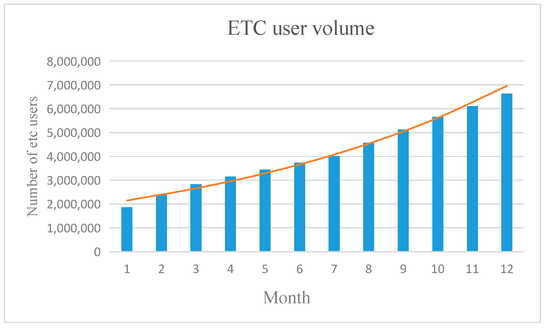
In previous studies, we found that demand price elasticity is inseparable from factors such as economy and geography. Even in different regions of China, people may have different attitudes towards a certain charge due to their different consumption customs. Therefore, when conducting a study of congestion charges in one region, it is unreliable to hastily refer to the elasticity of demand in other regions. The purpose of the research is to study the impact of the change in expressway charge price on the flow of cars with seven seats or fewer in Shanghai, China, through the demand price elasticity analysis method. The data come from the actual ETC charge data of Shanghai Expressway from 2019 to 2020. The data include the station information of vehicles entering and leaving the expressway, the charge amount, the vehicle type, etc. Based on this, we can obtain the traffic flow data between any two points. Due to government policy, the charging standard of the expressway has changed from 1 January 2020. Therefore, under this price change, the charge for vehicles on the same route has changed, and the change in traffic flow in 2019 and 2020 can provide data support for this research on the price elasticity of demand. Due to many factors that affect the change in traffic flow in 2019 and 2020, such as the growth of ETC users in 2019 and COVID-19 in 2020, in order not to affect the accuracy of the final result, this paper eliminates unknown factors except price through Empirical Mode Decomposition (EMD), and divides each path according to a different distance, so as to obtain the demand price elasticity of multiple OD pairs and analyze it. Figure 1 lists the growth level of ETC users in 2019. We can clearly see that there is an upward trend in Figure 1. This paper is divided into four chapters. The first part is the introduction, the second part is the methodology, the third part is the case studies and discussion, and the fourth part is the conclusion.
2. Methodology
2.1. Demand Elasticity
The elasticity of demand is a measure of the response of demand to changes in factors that affect it. Demand elasticity is an economic ratio without units, which can be defined as the ratio of the relative (percentage) change in demand scale to the relative (percentage) change in demand influencing factors. In general, it can be expressed by a formula. E represents demand elasticity, Q represents the demand, Xi indicates the demand impact variable, △Q indicates the amount of change in demand before and after, and △Xi indicates the amount of change in influencing factors before and after [15]:
It can be seen from the formula that there are positive and negative differences in demand elasticity. A negative value means that demand-influencing factors are negatively correlated with demand, and a positive value means that demand-influencing factors are positively correlated with demand.
When |E| > 1, demand is elastic to characteristics, and changes in characteristics will lead to substantial changes in demand, which means that demand is sensitive to this characteristic.
When |E| = 1, demand shows the characteristics of unit elasticity to characteristics, and the change in characteristics will lead to the change in demand by the same amplitude.
When |E| < 1, demand is inelastic to characteristics, and the change in characteristics can lead to low demand change.
When E = 0, it means that the demand is completely inelastic to the characteristics, and the change in characteristics will not change the demand.
Under the price elasticity of demand, X in the above formula represents the price, including but not limited to fuel fees, road charges, etc. The price in this paper refers to the expressway road charges.
2.2. Experimental Method
Due to the gradual demolition of toll booths at China’s provincial borders, the new toll collection standard was implemented on 1 January 2020. As a result, there is a change in expressway tolls between 2020 and 2019, which is the basis of this study. The original fee was to calculate the amount of the charge according to the actual mileage and then need to be rounded into an integer multiple of the billing unit (five yuan), but the current charging fee is calculated on the basis of the actual mileage. For example, before the actual mileage calculation to obtain three yuan, the actual charge was five yuan; now it is three yuan. The data of this study adopt the ETC charge data of Shanghai Expressway, and the time span includes the whole year of 2019 and June 2020 to December 2020. The data include the vehicle types of vehicles passing through the expressway, the entrance charge station, the exit charge station, and the charge amount. Based on the above background, by comparing the flow change rates in 2019 and 2020, we can find the price elasticity of road users’ demand for the expressway charges. It is worth mentioning that the change in the charging standard involves not only cars with seven seats or fewer, but also other types of cars. However, due to the change in vehicle classification standards, for example, vehicles originally belonging to two different types of cars will be divided into the same type of cars under the new standard (only cars with seven seats or less have not changed), which makes it impossible for us to accurately distinguish the type of cars of the flow. Therefore, in order to ensure the accuracy of the research results, we only study the demand price elasticity of cars with seven seats or less.
The data in the actual road network are used; therefore, there are many factors that affect the traffic flow. Two of the factors that affect the traffic volume are COVID-19 in 2020 and the surge of ETC users in 2019. Since these two known factors have a great impact on the traffic flow, we need to eliminate them in the follow-up study.
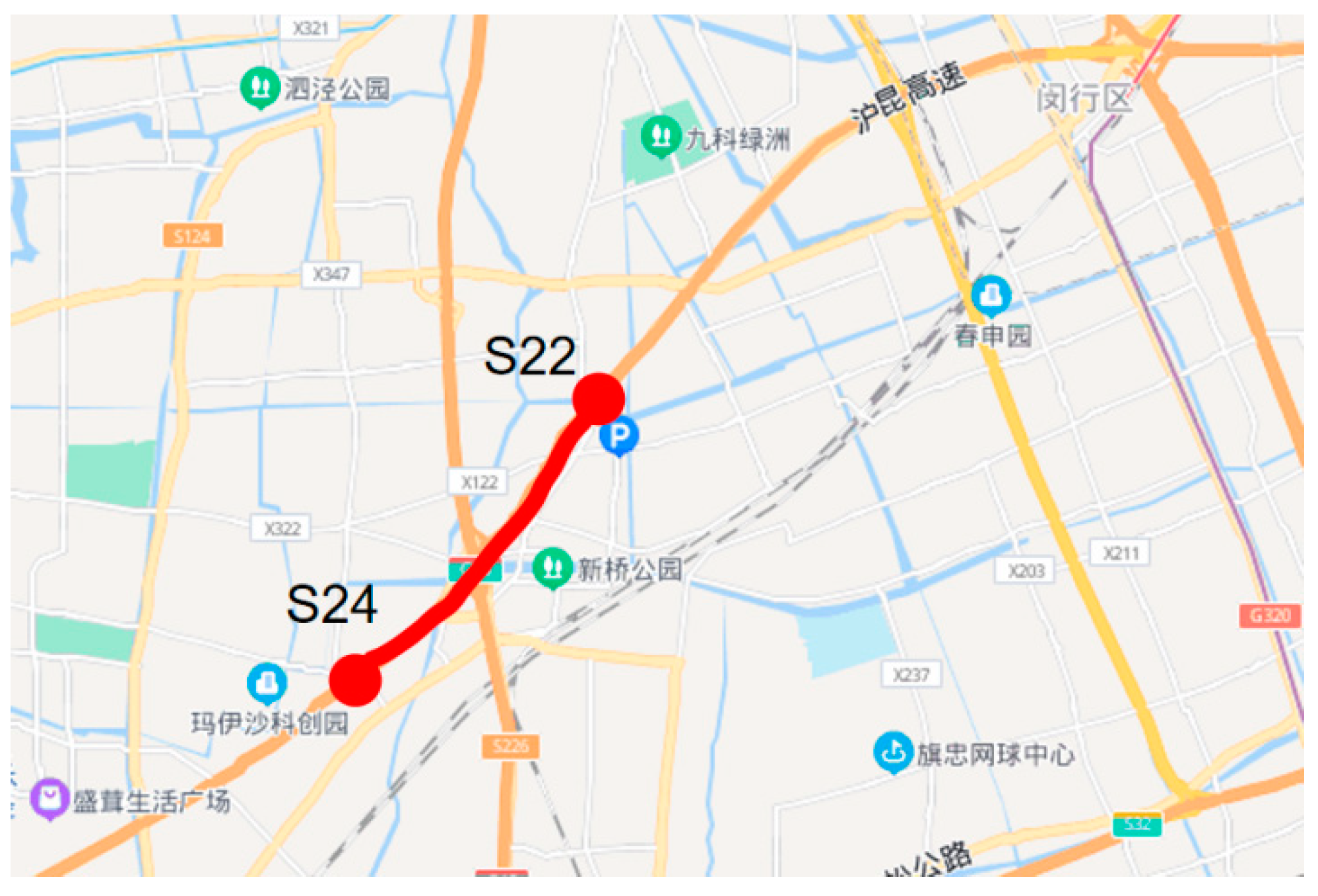
In order to eliminate the impact of the pandemic, according to the annual report of Shanghai’s comprehensive operation and transportation and the actual situation of the pandemic in 2020, since there are no new cases in Shanghai between June and October 2020, it is believed that the pandemic has the least impact on traffic flow during this period. The data from June to October 2020 and the ETC charge data of the same period in 2019 were used. Considering that expressway charges are related to mileage and starting and ending points, vehicles with the same starting and ending points have the same charging standard, which is conducive to the calculation of the price elasticity, this study adopts the OD one-to-one correspondence method. Vehicles with the same starting and ending points are put into two sets according to different years, so as to facilitate the subsequent comparison of the flow between the two sets. Since the data include all charge stations in Shanghai and some charge stations in other provinces and cities, they contains many OD pairs with less traffic. In order to prevent these OD pairs from affecting the final result, set the daily traffic threshold = 1000 pcu/d, exclude the OD pairs below this threshold, and obtain 29 OD pairs. For the convenience of article expression, OD pair names will be expressed in the form of numbers; for example, they will be expressed as S1, S2, S3, etc. Figure 2 shows the specific situation of an OD pair in the data. In Figure 2, the orange line represents the expressway, and the red line represents the route range of this OD pair.
Based on the objective fact that there is a substantial increase in ETC users in 2019, this will lead to abnormal calculation results of demand price elasticity; it is necessary to exclude the increase in ETC traffic caused by this factor when calculating the demand elasticity. This study uses empirical mode decomposition (EMD) to decompose the time series data into multiple time series data with different characteristics and frequencies. Therefore, the growth curve caused by the growth of ETC users can be found through the screened time series data. The growth curve obtained by EMD decomposition unifies the ETC user level from June to October 2019 to the October level. Since the curve includes monthly changes from June to October, in order to avoid the impact of monthly changes on the final results, this method is also used for normalization in 2020. At the same time, in order to avoid the impact of annual changes on the final results, according to the Shanghai comprehensive operation annual report, a report published by the government containing the coefficient of traffic flow growth from 2019 to 2020, multiply the data flow of each OD pair in 2019 by 6.1%.
Finally, we sum the daily data of each OD to obtain the total flow from June to October 2019 and June to October 2020 respectively, combined with the price change in each OD pair, the demand price elasticity of each OD pair can be obtained according to the demand price elasticity formula. In order to avoid different calculation results due to price increases or price reductions, the midpoint formula of arc elasticity in the demand elasticity formula is used to calculate the demand price elasticity of each OD pair, where Q1 and Q2 represent the demand before and after the change, and P1 and P2 represent the price before and after the change:
As mentioned earlier, the empirical mode decomposition (EMD) method is suitable for the analysis of both nonlinear and non-stationary time series data, as well as linear and stationary time series data. It can decompose the original signal into finite intrinsic mode functions (IMF).
The empirical mode decomposition method is based on the following assumptions:
(1) There are at least two extreme values in the data;
(2) The local time-domain characteristics of the data are uniquely determined by the time scale between the extreme points.
In order to decompose the eigenmode function from the original signal, the empirical mode decomposition method requires the following process:
(1) Find all extreme points in signal Z (T);
(2) Use a cubic spline curve to fit the envelope Emax (T) and Emin (T) of the upper and lower extreme points, and calculate the average value of the upper and lower envelope m (T), and subtract it from
Z (T): H (T) = Z (T) − m (T);
(3) Judge whether H (T) meets the requirements of IMF according to the preset conditions;
(4) If not, replace Z (T) with H (T) and repeat the above steps until H (T) meets the criterion, then H (T) is the IMFCk to be extracted;
(5) Every time you obtain a first-order IMF, deduct it from the original signal and repeat the above steps. Until the last part of the signal, rn is only a monotonic sequence or a constant sequence, which is called residual.
In this way, the original signal Z (T) is decomposed into a series of IMF and the linear superposition of residuals after EMD method decomposition.
To sum up, this method can exclude some cyclical trends and obtain more accurate internal trend lines, to further optimize the data.
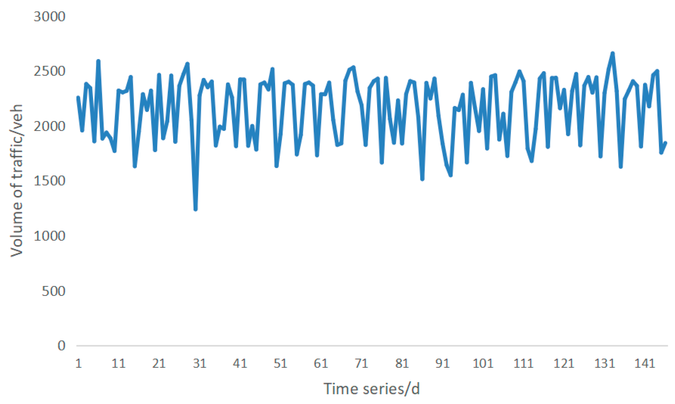
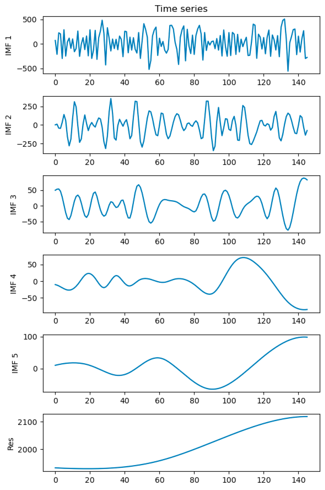
Figure 3 shows the annual traffic flow of an OD pair in Shanghai, and the Figure 4 shows the result of an OD after EMD treatment of traffic flow, where the abscissa represents the time series and the ordinate represents the result of addition and subtraction of the traffic volume. The five curves from top to bottom represent the five eigenmodes functions separated from the original traffic flow, and the last curve represents the residual after the isolation of the eigenmodal function.
As can be seen in the Figure 4, EMD divides the original data into six parts, and the residual part shows an obvious trend. In the previous study, we learned that the traffic flow has monthly changes in the annual changes. As mentioned above, due to the increase in ETC users in this data, the annual traffic has increased abnormally. Therefore, we can consider that the residual represents an overall trend after the combination of these two factors.
3. Case Studies and Discussion
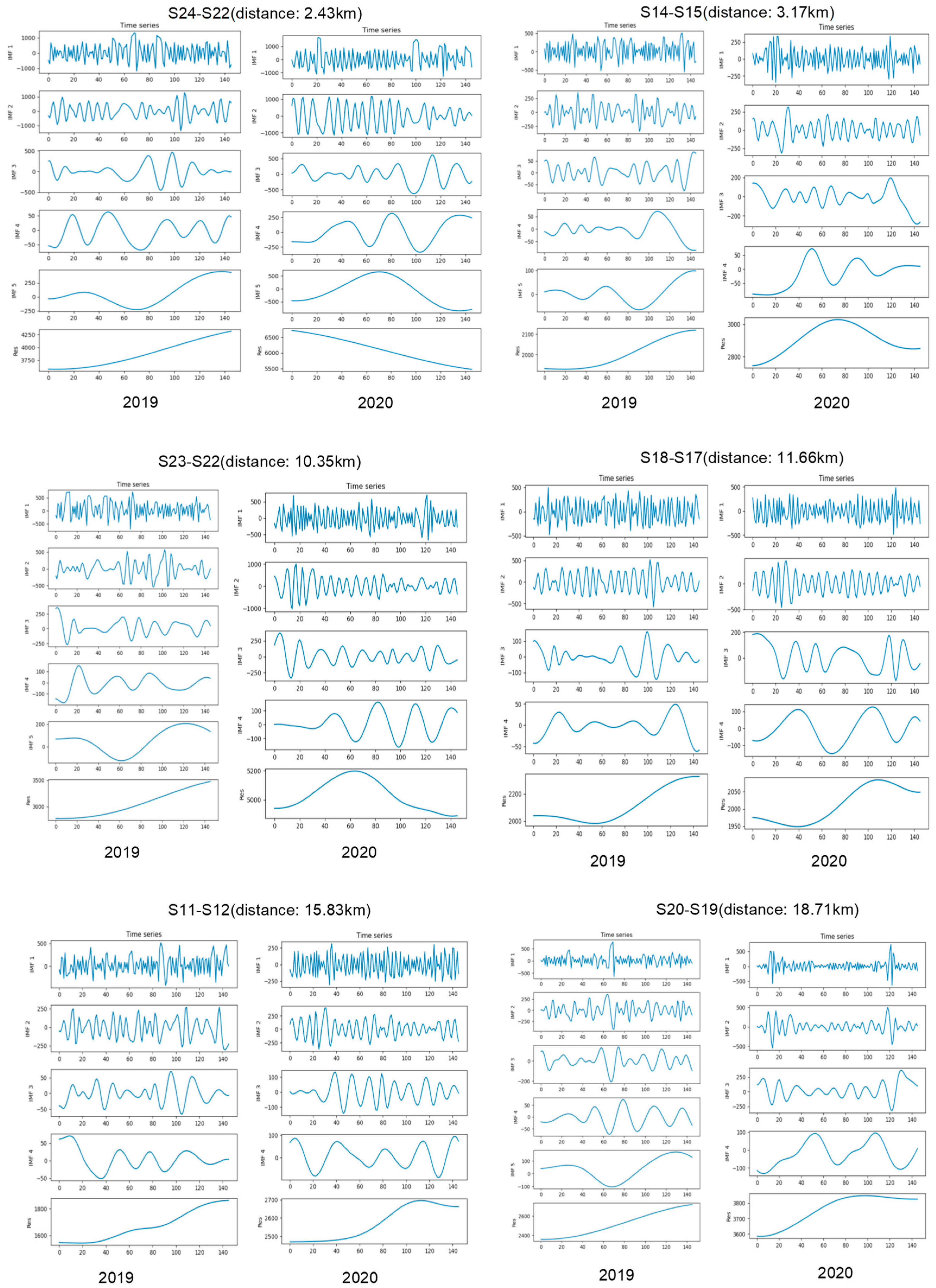
In this study, EMD is used to determine the internal trend of the ETC charging data of each OD pair. Due to space constraints, select OD pairs with different distances from 29 OD pairs for display, and the distance increases from left to right. In each group of graphs, the left side represents the result of the EMD decomposition of the OD pair’s 2019 traffic flow, and the right side represents the result of the EMD decomposition of the OD pair’s 2020 traffic flow. The abscissa is the number of days, and the ordinate is the traffic volume after decomposition. For example, in the first group, it represents the decomposition result of the OD pair (S24 to S22), and the distance between the two points is 2.43 km:
In Figure 5, we can find that the residuals of different years in each group are significantly different, while the residuals of the same year between groups have the same trend. This shows that it is correct to use the residuals separated by EMD to represent the trend of traffic flow change. The trend of traffic flow growth caused by the growth of ETC user level in 2019 has been shown in the figure above, but this factor does not exist in 2020, so the trend in 2020 mostly represents the monthly change in traffic flow. Next, we can smooth out the trend in 2019 by multiplying the traffic flow of each day by a factor to show that the level of ETC users in 2019 and 2020 is at the same level. However, this method also smooths the monthly change in traffic flow in 2019, which is not conducive to the calculation of demand price elasticity, so we also use this method for 2020 data. Therefore, we can think that among the factors that lead to the change in traffic flow, there are only charge changes. In order to maximize the use of these data, we sum the flow of each OD pair for 2019 and 2020 respectively. The price elasticity of demand is calculated through the midpoint formula of arc elasticity based on the charge difference between OD pairs.
Through data normalization processing, the elasticity value of each OD for passenger cars with seven seats and less is calculated according to the midpoint formula of the demand price elasticity arc as follows:
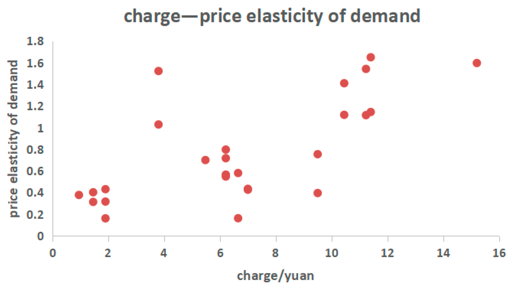
According to the definition of demand price elasticity, higher prices will lead to lower demand, the two OD pairs with positive demand price elasticity in the Table 1 obviously has other influencing factors leading to flow changes. To prevent such factors from affecting the research results, exclude the two OD pairs with positive elasticity in the above table, study the relationship between the remaining OD pair demand price elasticity and charge (distance), and take the OD pair 2020 charge (distance) as the abscissa, and the absolute value of demand price elasticity as the ordinate. The following figure is obtained:
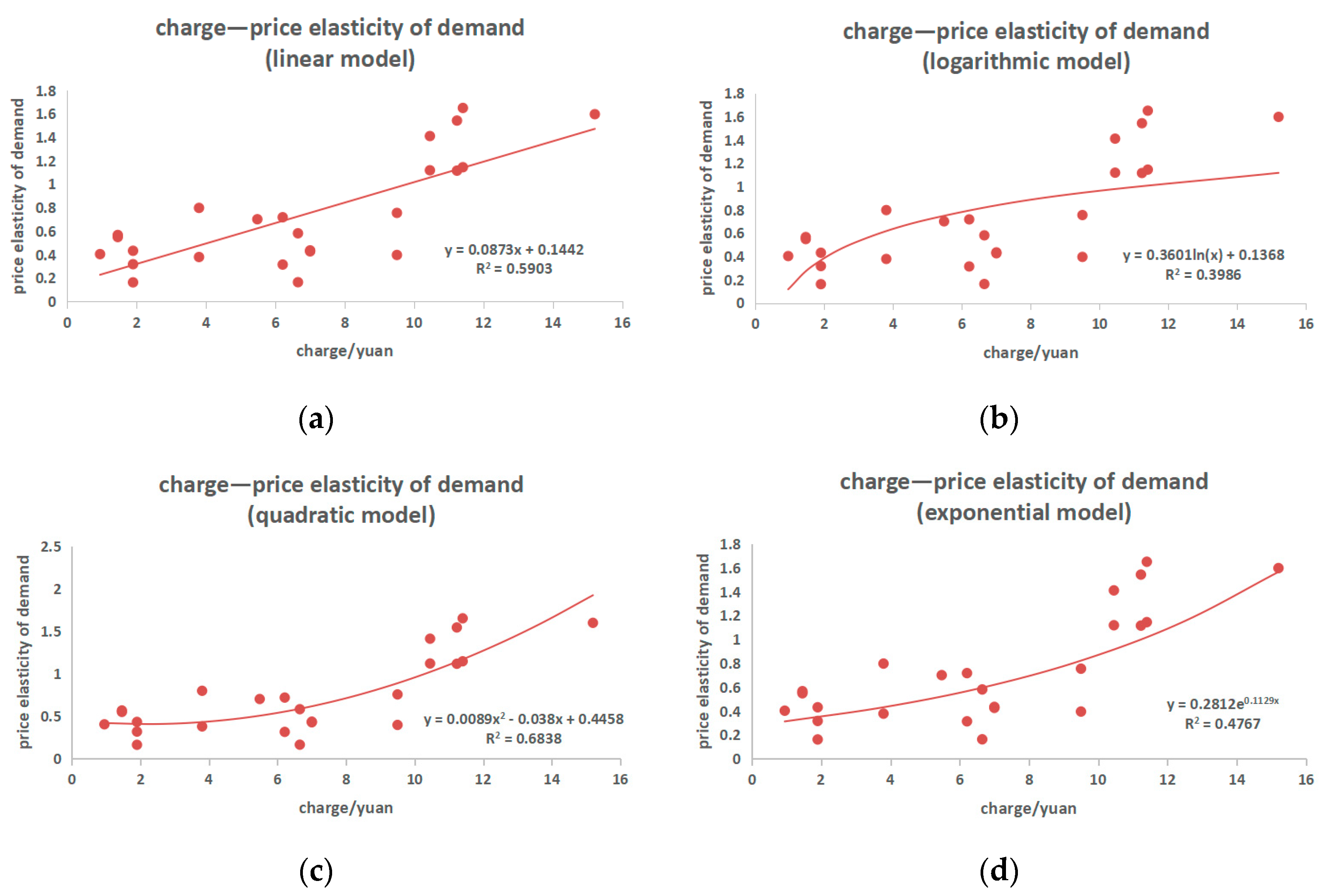
In the Figure 6, the abscissa of each point represents the charge amount of a certain OD pair, and the ordinate represents the demand price elasticity calculated from the traffic flow data of that OD pair, so we can see the change in demand price elasticity under different charges. In these points, it can be found that there are two discrete points deviating from the trend at the charge of 4 yuan. Among them, there is something in common with the two OD pairs that have been excluded in Table 1 that the charge difference is small. Therefore, the price elasticity of demand may not be accurate when the charge change is small. In this study, the change in these four OD pairs is less than 1 yuan. After excluding the above two discrete points, linear model, quadratic model, logarithmic model, and exponential model are used to regress the data, and their fitting results and goodness of fit R2 are obtained. Through the comparison of goodness of fit R2, the correlation strength between different elastic values and charges (distance) is obtained.
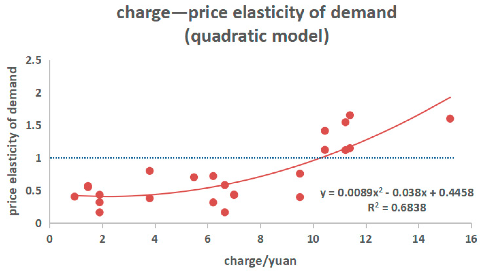
It can be seen from Figure 7 that the fitting accuracy of the quadratic model is the best, and it can be found that there is a negative correlation between the elasticity value and the expressway charge (travel mileage). The farther the travel distance is, the higher the charge is, and the greater the absolute value of the elasticity value is.
According to the definition of demand price elasticity, if the elasticity value is less than 1, it is inelastic, and if the elasticity value is greater than 1, it is elastic. In the Figure 8, when the charge is greater than 10.31 yuan, the elasticity value is greater than 1. Road users are more sensitive to price, and the implementation of road pricing is more effective in changing traffic flow. This shows that in short-distance travel, if the government wants to control the flow through charge, it needs a more aggressive charging strategy.
4. Conclusions
Based on the measured data, this study divides the road flow into multiple groups to analyze the demand price elasticity through the way of starting and ending points, and uses EMD to exclude the factors that have an obvious influence. Compared with other studies that calculate the elasticity value only through the change in traffic flow, this paper has a great improvement, the research results show that:
1. The demand elasticity of expressway charges is related to the number of charges. The longer the travel distance, the higher the charge, and the greater the absolute value of demand price elasticity;
2. In this study, road users with higher road charges are more sensitive to price changes, which shows that the effect of applying road charges in long-distance, high-charge cases will be better;
3. EMD has obvious advantages in analyzing the trend of time series data such as traffic flow. This study can provide some references for other research on the price elasticity of demand.
Author Contributions
The authors confirm contribution to the paper as follows: study conception and design: Y.L., M.S., L.S.; data collection: Y.L., M.S.; analysis and interpretation of results: Y.L., M.S.; draft manuscript preparation: Y.L., M.S., Writing—review and editing: X.W., S.S. All authors have read and agreed to the published version of the manuscript.
Funding
This research was funded by National Key Research and Development Project (2019YFE0112100), Science and Technology Innovation Action Plan of Shanghai Science and Technology Commission (21dz1203802), Science and Technology Innovation Action Plan of Shanghai Science and Technology Commission (20dz1202702), and National Natural Science Foundation of China (Grant No. 52272312).
Data Availability Statement
Data available on request due to restrictions e.g., privacy or ethical. The data presented in this study are available on request from the corresponding author. The data are not publicly available due to government policy restrictions.
Conflicts of Interest
The authors declare no conflict of interest.
References
- Olszewski, P.; Xie, L. Modelling the effects of road pricing on traffic in Singapore. Transp. Res. Part A Policy Pract. 2005, 39, 755–772. [Google Scholar] [CrossRef]
- TfL: Transport for London. 2003. Available online: http://www.cclondon.com/ (accessed on 16 March 2003).
- Burris, M.W. The toll-price component of travel demand elasticity. Int. J. Transport Econ./Riv. Internazionale Di Econ. Dei Trasp. 2003, 1, 45–59. [Google Scholar]
- Holguín-Veras, J.; Wang, Q.; Xu, N.; Ozbay, K.; Cetin, M.; Polimeni, J. The impacts of time of day pricing on the behavior of freight carriers in a congested urban area: Implications to road pricing. Transport. Res. Part A Policy Pract. 2006, 40, 744–766. [Google Scholar] [CrossRef]
- Holguín-Veras, J. Necessary conditions for off-hour deliveries and the effectiveness of urban freight road pricing and alternative financial policies in competitive markets. Transport. Res. Part A Policy Pract. 2008, 42, 392–413. [Google Scholar] [CrossRef]
- Holguín-Veras, J. The truth, the myths and the possible in freight road pricing in congested urban areas. Procedia-Social Behav. Sci. 2010, 2, 6366–6377. [Google Scholar] [CrossRef] [Green Version]
- Litman, T. Understanding Transport Demands and Elasticities. How Prices and Other Factors Affect Travel Behavior. (Victoria Transport Policy Institute: Litman). 2013. Available online: http://www.vtpi.org/elasticities.pdf (accessed on 22 November 2013).
- McKnight, C.E.; Hirschman, I.; Pucher, J.R.; Berechman, J.; Paaswell, R.E.; Hernandez, J.A.; Gamill, J. Optimal Toll Strategies for the Triborough Bridge and Tunnel Authority; Final Report; Triborough Bridge and Tunnel Authority: New York, NY, USA, 1992. [Google Scholar]
- Zou, W.; Wang, X.; Zhang, D. Truck crash severity in New York city: An investigation of the spatial and the time of day effects. Acc. Anal. Prevent. 2017, 99, 249–261. [Google Scholar] [CrossRef] [PubMed]
- Bari, M.E.; Burris, M.W.; Huang, C. The Impact of a Toll Reduction for Truck Traffic Using SH 130. Case Stud. Transp. Policy 2015, 2, 222–228. [Google Scholar] [CrossRef]
- Urbanek, A. Public Transport Fares as an Instrument of Impact on the Travel Behaviour: An Empirical Analysis of the Price Elasticity of Demand. In Challenges of Urban Mobility, Transport Companies and Systems; Springer Proceedings in Business and Economics: Berlin/Heidelberg, Germany, 2019. [Google Scholar]
- Sianturi, P.C.; Nasrudin, R.; Yudhistira, M.H. Estimating the price elasticity of demand for urban mass rapid transit ridership: A quasi-experimental evidence from Jakarta, Indonesia. Transp. Policy 2022, 10, 354–364. [Google Scholar] [CrossRef]
- Davis, L.W. Estimating the price elasticity of demand for subways: Evidence from Mexico. Reg. Sci. Urban Econ. 2021, 87, 103651. [Google Scholar] [CrossRef]
- Melo, P.C.; Sobreira, N.; Goulart, P. Estimating the long-run metro demand elasticities for Lisbon: A time-varying approach. Transp. Res. Part A 2019, 26, 360–376. [Google Scholar] [CrossRef]
- Holmgren, J. Meta-analysis of public transport demand. Transp. Res. Part A Policy Pract. 2017, 41, 1021–1035. [Google Scholar] [CrossRef] [Green Version]
Figure 1.
ETC user-level growth in 2019.

Figure 2.
Example of OD pair number.

Figure 3.
Example of raw data.

Figure 4.
IMF functions of different frequencies obtained after EMD.

Figure 5.
IMF functions of different frequencies obtained after EMD.

Figure 6.
Relationship between charge and elasticity value.

Figure 7.
Relationship between charge and elasticity value with model regress. Note: Subfigure (a) represents the fitting results using linear model, subfigure (b) represents the fitting results using logarithmic model, subfigure (c) represents the fitting results using quadratic model, subfigure (d) represents the fitting results using exponential model.

Figure 8.
Relationship between charge and elasticity value with quadratic model regress.


Table 1.
Elasticity value of each OD pair.
| OD Pairs | 2019 Charge/yuan | 2020 Charge/yuan | Distance/km | Charge Difference/yuan | Elasticity Value |
|---|---|---|---|---|---|
| S24-S19 | 4.75 | 0.95 | 1.58 | 3.8 | −0.42 |
| S22-S24 | 4.75 | 1.46 | 2.43 | 3.29 | −0.46 |
| S24-S22 | 4.75 | 1.46 | 2.43 | 3.29 | −0.37 |
| S14-S15 | 4.75 | 1.9 | 3.17 | 2.85 | −0.38 |
| S11-S16 | 4.75 | 1.9 | 3.17 | 2.85 | −0.50 |
| S15-S14 | 4.75 | 1.9 | 3.17 | 2.85 | −0.23 |
| S3-S21 | 4.75 | 3.8 | 6.30 | 0.95 | −1.78 |
| S21-S3 | 4.75 | 3.8 | 6.30 | 0.95 | −1.29 |
| S19-S26 | 4.75 | 5.23 | 8.72 | −0.48 | 2.17 |
| S26-S19 | 4.75 | 5.23 | 8.72 | −0.48 | 1.40 |
| S9-S10 | 9.5 | 5.48 | 9.13 | 4.02 | −0.81 |
| S22-S23 | 9.5 | 6.21 | 10.35 | 3.29 | −0.93 |
| S23-S22 | 9.5 | 6.21 | 10.35 | 3.29 | −0.86 |
| S22-S25 | 9.5 | 6.21 | 10.35 | 3.29 | −0.69 |
| S25-S22 | 9.5 | 6.21 | 10.35 | 3.29 | −0.71 |
| S5-S6 | 9.5 | 6.65 | 11.08 | 2.85 | −0.75 |
| S6-S5 | 9.5 | 6.65 | 11.08 | 2.85 | −0.33 |
| S17-S18 | 4.75 | 7 | 11.66 | −2.25 | −0.27 |
| S18-S17 | 4.75 | 7 | 11.66 | −2.25 | −0.28 |
| S11-S12 | 14.25 | 9.5 | 15.83 | 4.75 | −0.90 |
| S12-S11 | 14.25 | 9.5 | 15.83 | 4.75 | −0.54 |
| S3-S4 | 14.25 | 10.45 | 17.41 | 3.8 | −1.59 |
| S4-S3 | 14.25 | 10.45 | 17.41 | 3.8 | −1.30 |
| S19-S20 | 14.25 | 11.23 | 18.71 | 3.02 | −1.78 |
| S20-S19 | 14.25 | 11.23 | 18.71 | 3.02 | −1.36 |
| S7-S8 | 14.25 | 11.4 | 19 | 2.85 | −1.91 |
| S13-S11 | 14.25 | 11.4 | 19 | 2.85 | −1.41 |
| S1-S2 | 19 | 15.2 | 25.33 | 3.8 | −1.85 |
Disclaimer/Publisher’s Note: The statements, opinions and data contained in all publications are solely those of the individual author(s) and contributor(s) and not of MDPI and/or the editor(s). MDPI and/or the editor(s) disclaim responsibility for any injury to people or property resulting from any ideas, methods, instructions or products referred to in the content. |
© 2023 by the authors. Licensee MDPI, Basel, Switzerland. This article is an open access article distributed under the terms and conditions of the Creative Commons Attribution (CC BY) license (https://creativecommons.org/licenses/by/4.0/).
Share and Cite
MDPI and ACS Style
Li, Y.; Shao, M.; Sun, L.; Wang, X.; Song, S. Research on Demand Price Elasticity Based on Expressway ETC Data: A Case Study of Shanghai, China. Sustainability 2023, 15, 4379. https://doi.org/10.3390/su15054379
AMA Style
Li Y, Shao M, Sun L, Wang X, Song S. Research on Demand Price Elasticity Based on Expressway ETC Data: A Case Study of Shanghai, China. Sustainability. 2023; 15(5):4379. https://doi.org/10.3390/su15054379
Chicago/Turabian StyleLi, Yunyi, Minhua Shao, Lijun Sun, Xinmiao Wang, and Shizhao Song. 2023. "Research on Demand Price Elasticity Based on Expressway ETC Data: A Case Study of Shanghai, China" Sustainability 15, no. 5: 4379. https://doi.org/10.3390/su15054379
Note that from the first issue of 2016, this journal uses article numbers instead of page numbers. See further details here.