
Sustainable City Evaluation Using the Database for Estimation of Road Network Performance


Faculty of Business, Economics and Management Information Systems, University of Regensburg, Universitätsstraße 31, 93053 Regensburg, Germany
*
Author to whom correspondence should be addressed.
Sustainability 2023, 15(1), 733; https://doi.org/10.3390/su15010733
Submission received: 16 November 2022
/
Revised: 27 December 2022
/
Accepted: 29 December 2022
/
Published: 31 December 2022
(This article belongs to the Special Issue Sustainable Logistics and Environmental Protection)
Abstract
:This article introduces the Database for Estimation of Road Network Performance (DERNP) to enable wide-scale estimation of relevant Road Network Performance (RNP) factors for major German cities. The methodology behind DERNP is based on a randomized route sampling procedure that utilizes the Worldwide Harmonized Light Vehicles Test Procedure (WLTP) in combination with the tile-based HERE Maps Traffic API v7 and a digital elevation model provided by the European Union’s Earth Observation Programme Copernicus to generate a large set of independent and realistic routes throughout OpenStreetMap road networks. By evaluating these routes using the PHEMLight5 framework, a comprehensive list of RNP parameters is estimated and translated into polynomial regression models for general usage. The applicability of these estimations is demonstrated based on a case study of four major German cities. This case study considers network characteristics in terms of detours, infrastructure, traffic congestion, fuel consumption, and CO2 emissions. Our results show that DERNP and its underlying randomized route sampling methodology overcomes major limitations of previous wide-scale RNP approaches, enabling efficient, easy-to-use, and region-specific RNP comparisons.
1. Introduction
Road Network Performance (RNP) remains an integral part to the evaluation of urban sustainability [1,2,3,4]. According to Chen [5], the economy of a nation or geographic region depends heavily upon an efficient and reliable transportation system to provide accessibility and promote the safe and efficient movement of people and goods [6,7,8]. Poor RNP results in (1) decreased economical performance represented by increasing transportation costs [9,10,11,12], (2) negative ecological effects in terms of higher greenhouse gas (GHG) emissions [13,14,15] and (3) a decrease in social sustainability via a combination of the aforementioned factors in addition to traffic induced health issues [16,17,18,19,20]. Despite its importance for most aspects of everyday life [21,22] and its impact on productivity and costs of constantly increasing [23] short-distance freight operations [9,10,24,25,26], efforts on calculating RNP on a wide geographical scale remain scarce due to expensive equipment requirements for observational vehicles and so-called ‘in situ’ technologies [27,28]. Measurements are often restricted to predefined test tracks and restricted time intervals [29,30] and often fail to account for infrastructural and temporal variances throughout large road networks [20,25]. Furthermore, testing procedures may vary across cities and metropolitan areas, rendering them unreliable for systematic comparisons [31].
To solve several of these issues, analysts increasingly rely on digitization, specifically on open data platforms such as OpenStreetMap (OSM) and floating car data provided via Application Programming Interface (API) offered by navigation service providers such as HERE and TomTom, to estimate Road Network Performance on a wider scale by evaluating historical traffic data [23,29,32,33]. These digital procedures alleviate many problems encountered in field-testing, i.e., expensive equipment, regulatory hurdles, low area coverage, and low external validity [34], by leveraging the aggregated historical data of a large fleet of private and commercial vehicles [35]. Unfortunately, most navigation service providers require a set of predefined routes to enable the retrieval of route-specific information, leaving analysts to figure out sensible ways to either obtain historical traffic patterns on an individual basis or generate or extract such vehicle-specific data from publicly available information.
In 2020, Braun et al. [36] presented a data collection methodology to overcome the obstacle of route generation by referencing the TomTom Reachable Range API. The API returns a polygon with exactly fifty corner points covering the geographical area reachable within a given distance or time budget. This polygon enables a one-directional analysis of traffic patterns from an outgoing centroid, delivering time-specific information on reachable distances and corresponding travel time requirements within a region. Based on these requests, researchers were able to estimate road network characteristics on a per air-distance kilometer basis in an efficient way. By choosing comparable starting locations for multiple regions, RNP became observable and comparable between the exemplary four German cities. Nonetheless, this methodology introduced its own limitations, mainly concerning the selection of comparable points of origin and the impact of a good or poorly chosen node of origin on the model’s outcome. In addition to this major limitation, unidirectional routes ignore the fact that inbound traffic should be considered equally important for a generalizable RNP analysis.
To solve and remedy these shortcomings (i.e., unidirectional routes and subjective points of origin), a solution to algorithmically generate and evaluate a large set of representative network paths is required in order to establish a general road network performance measurement. To enable such a methodology, each path within a road network requires traffic information, but historically this has led to large amounts of API transactions [10,37]. By utilizing a novel and previously unavailable feature of the HERE Traffic API [38], access to real-time traffic flow data is provided for large geographic areas within a predefined bounding box via a single request. Since each request delivers geographically referenced information on speed and jam factors for all road sections contained within the specified region, this new feature enables the efficient generation and enrichment of routable road network representations. Based on this finding, we set out to answer the following research question, deduced from the original publication by Braun et al. [36]:
How can representative routes be generated and evaluated to reliably measure Road Network Performance and overcome limitations of contemporary RNP estimation?
The remainder of this article introduces and describes the methodology applied to generate the DERNP—the Database for Estimation of Road Network Performance in Germany. Section 2 examines the current state of RNP research and its lack of suitable, practical solutions. Section 3 presents the individual components utilized in generating and evaluating the underlying network routes of the proposed methodology. By aggregating all routes in a given region and distance class, DERNP includes polynomial regression coefficients to estimate factors such as detour, travel time and speed (with and without traffic), fuel consumption, and CO2 emissions based on a set air distance in a specific region. Section 4 demonstrates the applicability of these models by comparing four major German cities in terms of their economic and ecological sustainability. In Section 5, theoretical and practical implications are discussed. Section 6 summarizes the main takeaways of this article and provides an outlook for further research.
2. Literature Review
2.1. Fundamentals on Road Network Performance
Literature on transport pricing is well aware of the fact that poor Road Network Performance, generally defined as the network driven impact on sustainability [36] and mainly referred to in the context of traffic congestion, significantly reduces efficiency and increases transportation costs [9,10,39,40,41]. Specific negative impacts of traffic congestion, i.e., delays due to decreasing achievable travel speeds [42,43,44], economic losses to drivers [45], degrading ambient air quality [34,42,46,47] as well as general inconvenience and a reduction in quality of life [26] are well-researched topics in the literature. While traffic congestion can be subdivided into recurring and non-recurring traffic delays [39,48], i.e., regular and predictable road usage in comparison to road incidents such as collisions, medical emergencies, and vehicle breakdowns, studies on Road Network Performance tend to focus on recurring or general congestion patterns. To account for non-recurring traffic patterns, several studies have been carried out to allow for an improved estimation [49,50].
According to Mondschein and Taylor [51], geographic regions vary significantly in terms of adaption to traffic congestion. While congestion can constrain mobility and reduce accessibility, traffic is also associated with agglomerations of activity and is thus a byproduct of proximity-based accessibility. Whether agglomeration and congestion have net positive or negative impacts on activity participation thus varies substantially over space. In contrast to earlier studies of urban network performance focusing mainly on network reliability and resilience [5,52,53,54,55,56,57,58], this new perspective on RNP aims to provide geographically comparable measurements of Road Network Performance to supply indicators on regional attractiveness and infrastructural relevance [59].
In line with prior research [10,36] and supported by its predominant relevance for road freight transportation, we focus on the economic dimension of sustainability, which leads to a refined definition of RNP as the network driven economic costs of moving a vehicle from a specified point of origin (O) to a specified destination (D) using the public road network [36]. A public road network is characterized by the set of all roads within a geographical region that are accessible by all network participants and excludes private road infrastructure. To narrow down the scope of analysis presented in this article, the methodology is predominantly concerned with urban transportation, i.e., short distance traffic up to 20 km, also referred to as the last mile or urban cargo traffic [60,61].
In line with existing literature on road network transportation [9,10,39,42,43,44,46,53,62,63], we suggest measuring the geographically distinct Road Network Performance by answering the following general questions:
- How efficient is the road infrastructure in terms of detour factor and achievable travel speed?
- How utilized is the road infrastructure in terms of traffic congestion?
- How resource-intensive is the utilization of the road infrastructure in terms of fuel consumption and CO2 emissions?
Each of these questions is dependent on region-specific characteristics. Interestingly, as Bell [55] points out, network performance simultaneously depends on the state of the infrastructure and on the behaviour of network users, while user behavior is also governed by expectations about the general state of the network. Several studies have been carried out in support to this claim by examining and evaluating user behaviour in varying road networks. Milevitch et al. [64] apply agent-based traffic flow simulations to analyze the impact of planned road network development on the dynamics of the automobile transportation system during the departure of visitors after the semifinal match of the 2018 FIFA World Cup. Dia and Panwei [65] evaluate the impact of driving behaviour on emissions and RNP. Snelder and Calvert [62] propose the Macroscopic Dynamic Traffic Assignment and Marginal Model to evaluate the impact of weather conditions on driving behaviour and RNP.
In terms of infrastructure analysis, the detour factor, defined as the ratio of required road distance to cover a specific air distance, incorporates commonly used network attributes, such as density [66] or connectivity [67]. Travel speed is defined as the average speed achievable between origin and destination pairs considering vehicle and road constraints. Thus, travel speed implicitly accounts for road network attributes such as speed limits, traffic lights, or the level of congestion within the network [42,68,69] as well as user behaviour [55,65]. By combining travel speeds and travel distances, travel times can be derived [70]. Thoen et al. [71] show that longer travel times result in significantly higher transportation costs, emphasizing the importance of determining travel times objectively.
2.2. Leveraging Floating Car Data
Recent studies increasingly rely on floating car data in order to appropriately measure RNP. Kellner [28] analyzes vehicle fleet data from German transportation service providers to measure and compare network performance and its impact on distribution costs between different service areas. Nuzollo et al. [72] provide distribution tour simulations based on extracted floating car data from logistics operations, while Waadt et al. [73] present a methodology to estimate traffic congestion based on GPS data extracted from cellular networks.
Due to no generally accepted standard in floating car data extraction, the handling of these data are considered difficult. The large size of datasets and the complexitiy and dynamics of traffic phenomena [74] in combination with reliability problems [69] lead to increasing requirements of data harmonization [31]. Additionally, vehicle fleet management data is usually constrained to specific areas and routes serviced by the originating company, enabling region-specific analyses but prohibiting general measurements of RNP.
In recent years, increasing availability of floating car data provided by navigation service providers via APIs delivers potential solutions to efforts on data harmonization and regional specificity [75]. According to Kellner [37], API data is considered a significant improvement in contrast to individual data from fleet vehicle management systems due to four primary reasons: (1) Reliability or “completeness”, (2) area-wide coverage, (3) consistency, and (4) higher levels of representativeness. While APIs do not provide access to a complete set of individual routes due to privacy regulations, they record and deliver aggregated historic traffic information throughout many worldwide road networks in a structured query language. These databases enable researches to ignore primary data acquisition, shifting focus to automated generation or extraction of origin-destination pairs. Kellner et al. [10] referenced navigation service providers’ data to generate distance matrices for existing customers’ locations and requested travel times at different times throughout the day. Wen et al. [76] propose a traffic congestion evaluation index system based upon Beijing floating car data. In the same vain, Sun et al. [77] calculate a congestion index for arterial roads in Changzhou, China. Li et al. [78] obtain real-time travel data from web services to measure urban tourism accessibility in Nanjing, China. Nuzzolo et al. [72] analyze freight delivery patterns through floating car data in Italy while Waller et al. [79], comparable to Braun et al. [36], leverage data provided by TomTom, Google, and OSM to estimate RNP in Sydney through their Rapidex data exploration and visualization tool.
In an attempt to generalize methodologies presented in previous studies and alleviate many problems related to subjective trip generation, Braun et al. [36] suggest an improved approach to generalizable route generation based on real-world floating car data: for a given point of origin in the network, do not specify a destination and proceed to measure detour and travel speed for any origin-destination pair generated by a reachability approach using distance and time-based isochrones. While overcoming some limitations of previous research, especially concerning the availability of suitable or publicly available tour data, this methodology does not report RNP across the complete road network but manually selects well-defined partitions [80], constituting a lack of generalizability.
To the best of our knowledge, contemporary literature does not provide a suitable solution to the problem of limited individual route availability for wide-scale road network performance. By leveraging the HERE Maps API Version 7 [81] and its tile-based catalogue of historic traffic data in combination with publicly available OSM data on road network infrastructure [82], we propose a randomized route generation methodology which leverages floating car data and model-based traffic and emission simulation. The resulting Database for Estimation of Road Network Performance is inspired by the COPERT industry standard emissions calculator [83] and constitutes the first generalizable methodology for wide-scale RNP measurement for German metropolises. Our approach is considered efficient as the entirety of Germany can be analyzed by a total of 266 API calls per timestamp. Thus, DERNP allows measuring RNP on a large scale with no prior knowledge of origins and destinations and without a need to rely on second-best solutions, i.e., regional aggregation as suggested by Casadei et al. [84], alleviating a main concern of previous data collection methodologies.
3. Materials and Methods
The algorithmic measurement of RNP requires three main components: (1) a routable representation of the road network including all relevant public road sections in the area of interest, (2) traffic flow information for these sections, and (3) representative routes throughout the network along which the RNP is measured. The underlying methodology behind DERNP delivers solutions to acquire these components in combination with additional information to allow for an artificial generation of network traffic for any given area of interest. As depicted in Figure 1, the procedure consists of five phases.
3.1. Phase 1: Data Collection
The exemplary use cases in this article focus on German cities by defining the area of interest as the outermost rectangular boundary of any given city. To harmonize extraction procedures across data providers, DERNP relies on the commonly used, web-based Slippy Map Tile system [85]. Based on a list of required tiles per bounding box, a routable representation of the road network within the tiles is created using the OSMnx Python package [86]. This representation only includes user-generated data from the OSM community [82], which is prone to be incomplete, outdated, or incorrect. To alleviate this issue, the HERE Traffic API [81] is utilized to retrieve current traffic flow information on a per-tile basis. All tile references in this article rely on a set of HERE traffic data retrieved in between 25 July 2022 and 10 September 2022 at five different timestamps (08:00 a.m., 09:00 a.m., 12:00 p.m., 02:00 p.m., and 04:00 p.m.). Traffic data is held constant for purposes of reproducibility within this article but should be updated in regular intervals. The selected time frames are related to main working hours of German Transportation Service Providers. Additional time frames can be considered if relevant to the underlying business case. Figure 2 and Figure 3 depict fluctuations of averaged flow speeds between the four exemplary German cities during this time frame. Exact results can only be guaranteed by referencing identical data at identical timestamps across all objects of comparison [54].
Concerning nomenclature, a network’s free flow state describes the traffic flow without congestion exceeding an agreed upon norm [87] and corresponds to the average historic travel speed without extraordinary traffic incidents. Comparing free flow and traffic speeds at 08:00 a.m. on a specific date results in an indicator whether or not the inspected date is representative of average network usage or if higher-than-average traffic is occurring. Comparing free-flow speeds between different areas at the same timestamp provides a good indicator of average road network performance between geographies.
Using OSMnx [86], the network is initialized as a dynamic graph object [88] consisting of nodes and edges. Traffic flow data is mapped onto this graph based on latitude/longitude coordinate pairs. The mapping is validated by comparing the edge length attribute of both input sources.
The last information added onto the graph object is elevation data extracted from the digital elevation model provided by the European Union’s Earth Observation Programme Copernicus [89]. To achieve compatibility with the given network structure, global elevation data provided in .tff format is converted into tile-based raster files.
Successful application of Phase 1 results in a Routable Road Network (RRN).
3.2. Phase 2: Network Rasterization
During network rasterization, the RRN is subdivided into a grid of 150 × 150 equally-sized cells. Each cell is geographically referenced using the same coordinate reference system as the RRN. The centroid of each cell represents a point defined via latitude/longitude coordinate pairs.
Due to the high level of subdivision created by 150 × 150 grid cells, the smallest distance between two centroids is measured at 150 m air distance for large cities like Munich. Based on this grid, a distance matrix between all centroids is calculated using the great-circle distance formula, resulting in a matrix of air distances c between all centroid pairs. Based on this distance matrix, randomized route sampling with a default sample size of is applied to extract observations for each distance class. Distance classes for this study range from 500 m to 20.5 km air distance in increments of 500 m, resulting in 40 distinct classes.
Random route sampling enables the independent selection of travel path connections across the entire network for each distance class. These travel paths need to be converted from direct air connections to actual vehicle routes utilizing the existing Routable Road Network. Non-routable connections are dropped.
Network rasterization returns a dictionary containing a key for each distance class and a list of artificial network paths as corresponding value.
Figure 4 depicts the complete graph for Munich in comparison to the graph that is traversed by all paths within the network rasterization dictionary generated using random route sampling. While smaller road segments are left out due to not being located on any fastest path between two nodes, the majority of arterial roads are covered and can therefore be utilized in calculating the RNP in the subsequent steps.
3.3. Phase 3: Route Generation
The network paths returned by the previous step correspond to the fastest path from origin to destination, while these paths are sufficient to calculate average travel speed under free flow and traffic conditions, realistic estimation of RNP in terms of economical and ecological sustainability requires representative driving cycles. To achieve realistic measurements without excessive field testing, the Worldwide Harmonized Light Vehicles Test Procedure (WLTP) [90] is the standardized testing scenario for new vehicles since 1 September 2019. It includes a highly detailed set of representative driving cycles on a 1 Hz (per second) basis.
By referencing the WLTP, custom driving cycles are calculated for each network route. Although not perfectly accurate, especially on shorter road segments, these driving cycles do allow for a much more realistic representation of actual driving behaviour than mean speed calculations. A customized driving cycle for a 2.1 km route in Munich is depicted in Figure 5.
By applying the customized driving cycle logic to all routes in the dictionary returned in Phase 2, a Driving Cycle Catalogue (DCC) comprised of up to 40,000 estimated driving cycles across all 40 distance classes is generated.
3.4. Phase 4: Route Evaluation
All driving cycles in the DCC simulate real-world network paths throughout the RRN, including acceleration and deceleration phases as well as stop times (speed = 0 kph) at intersections or traffic lights. This information is crucial since the number of existing intersections in a road network is heavily flow-regulating [91].
To achieve a realistic measurement of RNP, it is therefore mandatory to take specific driving behaviours and road characteristics into account instead of relying on averaged calculations. It is due to this that we dissuade from referencing COPERT emission curves [83] and instead focus on the cycle-based Passenger Car and Heavy Duty Emission Model (PHEM) [92]. An Open-Source version of PHEM tailored to Microscopic Traffic Simulation titled PHEMLight is available in the software package SUMO [93,94]. For application in the DERNP methodology, PHEMLight Version 5 was transposed to the Python programming environment. In its Creative Common License, PHEMLight only includes two vehicle types: light passenger vehicles rated EURO 4 for both gasoline and diesel engines. Due to this, all calculations presented in this article are based on a standardized EURO 4 Diesel Light Passenger Vehicle with a rated power of 74 kW, belonging to the WLTP Class 3.
3.5. Phase 5: Transformation
After evaluation of all 40,000 driving cycles using PHEMLight5, results are saved in a tabular structure. Individual data points are aggregated by their corresponding distance class using a median calculation, resulting in a table of 40 rows with one column per network performance factor as described in Table 1. Based on these aggregated results, 10th-degree polynomial regression curves are fitted for each factor to enable continuous approximation on the basis of air distance.
After successful transformation of all included factors, the DERNP reference database for the six largest German cities is depicted in Table 2. Additional cities or customized areas of interest can be calculated using the methodology described above. To calculate a specific factor F for a given air distance in kilometers, coefficients from columns a to k need to be inserted into a 10th-degree polynomial function (Equation (1)).
4. Results
The DERNP (Table 2) allows for fast and efficient regional comparisons in terms of economical and ecological RNP. Since DERNP relies on air distance measurements as input factors, it seamlessly integrates into existing calculation models. To visualize the impact of differences in RNP between geographical regions, the upcoming section examines four of the largest German cities: Berlin (North-East), Hamburg (North), Stuttgart (South-West), and Munich (South-East). These cities rank highly in the 2021 TomTom Traffic Index [95] but vary significantly in terms of road network size.
Figure 6 visualizes the size differences in road network length (measured in kilometers) and the total length of network kilometers traversed for the DERNP generation. Due to the fixed amount of 40 distance classes and the fixed number of generated paths per distance class, larger networks feature less coverage than smaller road networks. Additionally, as depicted in Figure 4, DERNP, due to being based on fastest network paths, focuses on larger, arterial roads within networks and tends to ignore smaller residential roads. Even though these smaller roads make up for a large amount of total network length, they can be considered less important for overall RNP as they are less likely to be traversed by a large number of vehicles.
4.1. Detour Factor
The detour factor (Equation (2)) is defined as the increase in road or travel distance compared to a straight-line connection using air distance and measures the infrastructural efficiency of a road network. The less turns and intersections required to overcome a specified air distance, the better the detour factor. A perfectly straight road without turns or intersections corresponds to a detour factor of 1.0.
Figure 7 indicates that all investigated detour factors follow a similar pattern. Short distances in a large city introduce a heavy detour penalty due to the densely populated inner-city areas. As air distance increases, larger surrounding roads, also known as arterial roads, are accessible, significantly decreasing the detour necessary to cover air distance. The curve for Hamburg is noteworthy, as it decreases less rapidly compared to the other curves. This indicates a strong deviation from a road network made up of straight connections, which is certainly the case in the city of Hamburg due to the river Elbe and its many waterways inside the inner-city area. Interestingly, Munich’s detour factor is significantly lower up to 10 km air distance, indicating a well-built road infrastructure which allows for more direct connections. While Stuttgart’s road infrastructure appears to be comparable up to 8 km air distance, a bump can be seen upwards of 10 km air distance. This indicates a below-average road infrastructure at the outer city boundaries, coming close to Hamburg’s detour factor. This phenomenon is caused by the city’s geographical location within the valley basin of Stuttgart and its unusual city area which extends over an altitude difference of almost 350 m.
4.2. Fuel Consumption and Impact of Network Elevation
The unusual geographical situation in the Stuttgart city area is further supported by examining the fuel consumption per air distance kilometer. As can be seen in Figure 8, Stuttgart shows a significantly decreased fuel consumption curve both for (a) the total and (c) the average fuel consumption. This observation is caused by the PHEMLight5 emission calculation methodology which reports a less steep increase in fuel consumption for positive slopes in comparison to its coasting fuel consumption on negative inclines. Therefore, vehicles in areas containing large changes in altitude can save a disproportionately high amount of fuel while coasting in comparison to the increased fuel consumption caused by traversing positive slopes within the network. This hypothesis is further validated by examining Figure 9, which depicts the absolute and relative difference in fuel consumption caused by including elevation parameters in the PHEMLight5 calculation model.
Besides Stuttgart, the city of Berlin introduces another interesting observation in terms of fuel consumption. While Hamburg is the most fuel-intensive city for short distances, Berlin overtakes at both in (a) actual and (c) average fuel consumption. This indicates that while most of the inspected cities enable more efficient driving behaviour at longer air distances, Berlin fails to achieve this effect. This is caused by the much larger network size of Berlin compared to the remaining three cities (Figure 6), corresponding to a larger diameter of the inner-city area where intersections and traffic stops are much more frequent, resulting in a higher subdivision in driving cycles. This increase in subdivisions, equaling a higher number of stops and acceleration/deceleration phases, significantly increases fuel consumption, rendering driving in Berlin less fuel efficient.
4.3. CO2 Emission
In addition to fuel consumption, PHEMLight5 includes common emission calculation models based on driving cycles, including Nitrogen oxides (NOx), carbon monoxide (CO), hydrocarbons (HC), particulate matter (PM), particle number (PN), and carbon dioxide emissions (CO2). This information enables potential CO2 compensation calculations on a per-vehicle-kilometer basis. Since CO2 emission per liter Diesel can be described by a ratio of kg/L [96], the emission curves depicted in Figure 10 follow the same general behaviour as their fuel consumption counterparts (Figure 8), leading to identical interpretations. Nonetheless, we include the emission curves for ease of access to CO2 emission information.
4.4. Speed Profiles and Travel Times
Speed profiles and travel time curves provide information on how cities position in terms of infrastructure and congestion measurement. A well-built infrastructure enables longer coasting and less stop times, leading to more efficient driving cycles and a decrease in travel time per air distance kilometer. High levels of congestion decrease the achievable average velocity during these driving cycles, leading to an increase in travel time.
Figure 11 depicts achievable travel speeds for each distance class in (a) free flow and (b) congested state as well as (c) the traffic-induced relative decrease in average velocity. Figure 12 focuses on the corresponding travel times.
In both free flow and congested state, the city of Hamburg is among the top curves in terms of achievable travel speed. When looking at the traffic penalty curve for Hamburg, the relative increase in travel time (Figure 12c) caused by traffic congestion peaks at 17 percent or, in other terms, an average increase of min when covering 20 km air distance. This indicates that Hamburg suffers from a comparatively low congestion level among most of its network paths, which is in line with average speeds depicted in Figure 2 and Figure 3. Nonetheless, travel times remain similar to the remaining cities, which is largely caused by the poorly designed infrastructure due to the river Elbe as depicted by Hamburg’s detour factor (Figure 7).
Interestingly, the city of Berlin suffers the least from congestion (15 percent peak or min at km) while achieving the slowest travel speed in free flow and the second-to-last travel speed in congested state. Based on this observation in combination with an average detour factor, it appears that Berlin suffers from an almost constantly high level of congestion, influencing the historic free flow speed and significantly reducing the gap between free flow and congested state.
The counterexample to this is Stuttgart. While the travel speed during free flow is akin to Hamburg, it drops significantly when accounting for traffic within the observed time frame, requiring an additional 12 min to achieve the same distance of 20.0 km. This effect is also displayed in the relative traffic penalty curve for Stuttgart, with a relative traffic induced time penalty peaking at 30 percent.
The cities displaying the largest variation between free flow and congested state are Munich and Stuttgart, with Stuttgart showing a constant increase in relative loss compared to free flow, indicating a large congestion problem throughout the entire city. Munich, on the other hand, is characterized by an increasing level of relative loss or penalty up to a plateau value of 21 percent (difference in velocity) and 23 percent (traffic induced penalty) where it remains constant. This indicates a large congestion problem for short to medium length travel distances, implying a high level of traffic in inner-city areas, while longer paths upwards of allow for improved traffic flow, which might imply access to larger roads with less congestion on the city boundaries.
4.5. Transportation Costs
The economic dimension of sustainability of infrastructure, congestion, and detour factor is reflected in total costs of transport. In addition, DERNP allows translating environmental sustainability into economical impact by proposing the inclusion of CO2 compensation costs into transport cost evaluation. The price per ton CO2 is set to EUR 180, in line with current political debates by the German Federal Environment Agency [97]. Additionally, we assume EUR 0.7 per kilometer driving costs, an hourly wage of EUR 20.5 as driver costs and EUR 7.5 per hour of vehicle occupation costs, which is in line with other literature [98]. In contrast to comparable studies and based on their heavy impact on transportation costs [99], fuel costs are split from distance-based costs and incorporated on the basis of estimated vehicle fuel consumption derived from PHEMLight5 with a price per liter for Diesel fuel of EUR 1.70.
Figure 13 depicts the conglomeration of individual costing factors (a) to (e) in EUR per air distance which account for total costs of transportation in (f) free flow and (g) congested state. Subplot (h) depicts the difference in transportation costs caused by traffic congestion. Free flow data was compared to average traffic data for each city in between July 25 and September 22 of 2022. Traffic-specific results may vary for different time frames. Free flow data constitutes the historical average and is resilient to changes in specified time frames.
The total costs of transportation per air distance kilometer are highest in Hamburg and Berlin both in free flow and congested state. While Hamburg suffers from less travel time loss compared to Berlin, the difference is equalized by an increase in travel distance and distance related costs due to inefficient infrastructure as measured by the detour factor. Since both fuel and CO2 compensation costs correlate only with travel distance, both Hamburg and Berlin inflict a disproportionate cost surplus in comparison to Munich and Stuttgart.
With the exception of fuel and CO2 compensation costs, transportation is most cost-efficient across all cost components in the city of Munich. A low detour factor due to well-built infrastructure in combination with comparably less congestion and better optimized free flow conditions allow for savings of up to EUR 0.6 per kilometer air distance in Munich compared to Hamburg.
Stuttgart, on the other hand, inflicts higher distance and time related costs than Munich but saves significantly in terms of fuel and CO2 compensation due to increased coasting possibilities based on its geographical location. Nonetheless, even combined, these savings account for no more than one-third of total distance-related costs, resulting in transportation costs slightly higher than in the city of Munich both in free flow and congested state.
Subfigure (h) depicts the difference in costs per air distance between historical network speeds (free flow) and measured traffic speeds (congestion) within the specified time frame. As explained earlier, Berlin appears to suffer from a constant state of congestion, diminishing most differences between free flow and congested travel speeds. Stuttgart, on the other hand, seems to suffer from a more temporary congestion problem during the seven weeks of observation, accounting for a difference in transportation costs of up to EUR 0.14 per air distance kilometer on short paths. As path lengths increase, the difference between free flow and congestion rapidly decreases due to an increase in availability for alternative routes and faster arterial roads. Converging onto EUR 0.01 per kilometer for paths upwards of km, differences become negligible, removing the need of accounting for time-specific traffic conditions.
5. Discussion
The methodology presented in this article adapts and improves on existing methodologies by generating a large set of representative and realistic driving cycles to enable RNP measurement for any geographical bounding box, as long as OSM and HERE Traffic data is available. It therefore manages to overcome a major limitation of previous RNP iterations, which directly depended on a subjective selection of starting locations [36]. The resulting network coverage upwards of 59 percent for most large German cities presents a considerable leap in applicability in comparison to existing studies.
Results derived from the DERNP are in line with comparable studies, such as the TomTom Traffic Index [95] or an RNP approach based on reachable range isochrones [36]. By leveraging the PHEMLight5 [93] emission framework, DERNP provides the first catalogue of combined economic and environmental parameter estimators based on simple air distances. The inclusion of CO2 compensation costs for sustainable transportation costing based on specific regional geographies can lay the foundation for more realistic and comprehensible approaches to dynamic costing. Studies on the acceptance of congestion pricing indicate that environmental sensitivity is one of the most influential factors that positively affect the acceptability of transport charging policies [100]. As environmental sensitivity can be expected to continually increase over the next decade [101], so does the relevance of CO2 and congestion pricing strategies [102].
By incorporating realistic driving cycles based on the Worldwide Harmonized Light Vehicles Test Procedure, DERNP manages to improve upon static, mean-based fuel consumption methodologies commonly found in previous studies [36,103,104]. Customized driving cycles provide a better estimation of actual traffic behavior as they account for the amount of traffic lights, intersections, roundabouts, and other flow-regulating infrastructural characteristics which are especially important in urban transportation. Our study shows that topology varies heavily between geographic areas, resulting in higher or lower traffic efficiencies and increased or decreased travel costs.
The same is true for the inclusion of elevation data. Even though most major German cities do not contain high variation in geographical elevation, the city of Stuttgart provides a case in point that elevation data, especially in combination with highly detailed emission models such as PHEMLight5, can lead to significant differences in fuel consumption and CO2 emissions [105].
In addition to the aforementioned aspects, the DERNP confirms and further supports many findings of prior studies on RNP. As previously described, the free flow state in any network includes an accepted delay [87,106]. Even during free flow state, the maximum allowed speeds are mostly unachievable. This is mainly due to a certain number of simultaneous road users that are considered acceptable during any given time of day. Additionally, certain characteristics of existing infrastructures such as road conditions, traffic lights, and traffic routing considerably influence the maximum speed any road user can be expected to reach. Traffic congestion therefore is not defined by a speed lower than the maximum speed, but as the excessive delay above an agreed upon norm [36].
It remains true that little attention has been paid to the explanation of the detour factor, its determination, and its influencing factors. Nonetheless, our study shows its importance for transport costing as it significantly impacts the cost per air distance kilometer due to the high share of distance-based costs in comparison to total costs of transport. In accordance with previous studies [36], the detour factor decreases with increasing air distance throughout urban areas. This effect is a direct result from the existence of motorways or inner-city highways. These more efficient sections of road networks usually follow a comparably straight or direct course and can be accessed with a higher likelihood as air distances increase. Consequently, when calculating costs, transport companies must take a closer look at short distances, as the costs per kilometer can be many times higher than for longer distances. These short distances occur mainly in distribution between customer locations.
Special care has been taken to account for recent developments in fuel pricing. Previous studies tend to aggregate fuel costs into distance-based costs, obscuring the impact of external fuel price changes and internal cost factors. DERNP deliberately splits and disaggregates distance-based costs from fuel costs, allowing for a better evaluation of internal performance and external, non-adjustable effects.
In general, Section 4 underlines the fact that significant cost differences can arise between different geographical regions. As a practical example, since transport companies mostly charge prices for distribution independent of regional characteristics, the contribution margin of a single shipment might vary significantly between regions [10,36]. When comparing costs between business units, care should be taken to account for differences in geographical characteristics by referencing the DERNP and adjusting expectations accordingly, i.e., via proportional corrections based on comparative RNP measurements.
In contrast to prior research [36,103], DERNP does not define the free flow state by measuring traffic speeds at night. Instead, free flow and traffic speed are compared at identical timestamps, allowing for a comparison between average historic network performance and current network utilization. Most transportation services do not occur at night, rendering free flow results measured during closing hours irrelevant. To allow for a better estimation of traffic costs, the average network performance during delivery hours adjusted by current real-time traffic attributes should be taken into account. Interestingly, when applying the DERNP logic, differences between free flow and congested state diminish in many cases since major German cities tend to suffer from a constantly high level of traffic congestion. Due to this, free flow and congested network performance converges during the relevant business hours.
6. Limitations and Further Research
While digitization and open data platforms, such as OSM, provide researchers and analysts with large sets of data, the validity of such crowd-sourced data is a matter of concern. DERNP implements multiple types of validity checks, especially for calculated road attributes. Nonetheless, it fails to account for correctly inserted information by content creators. Several studies found that OSM data is mostly accurate for densely populated areas in developed western countries while accuracy decreases significantly for less developed regions [107,108,109,110,111,112]. Further studies might be necessary to validate these claims, especially for German road infrastructure referenced during this study as it represents the backbone of the proposed methodology.
In addition to OSM data, traffic information retrieved from the HERE Traffic API is another point of contention concerning the validity of the presented results. In general, further research should evaluate differences in historic traffic data between HERE and other navigation service providers, such as TomTom or INRIX. On a more specific note, external validity could be improved by incorporating additional timestamps throughout the day besides the five timestamps used in this study (08:00 a.m., 09:00 a.m., 12:00 p.m., 02:00 p.m., 04:00 p.m.), albeit at an increase in API requests and the costs associated with it. This change would also allow for a better estimation of isolated infrastructural impact, as performance deterioration inherently caused by network participants can be omitted or minimized at less populated timestamps such as 03:00 a.m. as was shown in previous studies [36].
In the same vein, the selected time frame of 25 July to 10 September, 2022 covers the time period of summer vacation for most German states, which might distort the results observed. At the time of writing, the HERE Traffic API does not allow extraction of historic timestamps, severely limiting the availability of data without this distortion. Future research might investigate potential seasonality in network utilization, validating or refuting such concerns.
Another limitation to the validity of the provided results can be seen in the novel approach to driving cycle generation based on the WLTP. While the WLTP certainly provides accurate estimations for laboratory studies in vehicle emission behaviour, the applicability to real-world driving scenarios requires additional research. As Greenwood [113] points out, predictions of fuel consumption based on generated driving cycles may differ by up to 25 percent in comparison to data extracted from equipped single cars. Due to this, future studies should focus on validating and improving the customized driving cycles contained within the driving cycle catalogue by extensive field testing or comparative studies. Introduction of a smoothing factor to allow for better merging of individual road sections might improve accuracy to real-world driving behaviour.
In its current version, DERNP only includes RNP estimators for EURO 4 light passenger vehicles. While general performance patterns between cities will likely remain identical, specific emissions and cost factors will change significantly when incorporating modern engine models as well as heavy duty vehicles. Therefore, future research should focus on acquiring modern vehicle models and updating the provided results, either via licensing through TU Graz or by independent generation of suitable vehicle data.
As DERNP is meant as a generic and universally applicable database for RNP estimation, it tries to measure RNP across the entirety of a road network. While theoretically correct, in practice most transportation service providers, commercial or public, will traverse the same subset of individual network paths multiple times per week or day during operation, rendering generic results less representative for specific service areas. Future studies should focus on acquiring and comparing historic vehicle fleet data for specific service areas to general results provided by the DERNP to measure practical applicability in a more comprehensive study. More specifically, DERNP results should be compared to commercial solutions such as PVT Vissim in order to acquire a reliable benchmark for representativeness of open source solutions in comparison to established commercial software packages.
In addition to these proposed changes, research should focus on identifying potentially missing latent parameters relevant to RNP (besides detour, infrastructure, traffic, and elevation), which are not included in either the current or any previous iteration of RNP measurements. Exploratory studies might also be valuable in incorporating the last remaining dimension of social sustainability into RNP measurements. As a starting point, DERNP enables the inclusion of vehicle noise emission frameworks such as CoRTN or CONOSSOS on the basis of highly detailed 1 Hz customized driving cycles included within the driving cycle catalogue. By combining all required information to implement these frameworks, our method can help to quantify the impact of RNP on urban social sustainability.
7. Conclusions
The contribution of this paper is the presentation of an efficient methodology to generate a large set of representative individual driving cycles through OSM road networks by referencing the Worldwide Harmonized Light Vehicles Test Procedure. Based on this driving cycle catalogue, the reference Database for Estimation of Road Network Performance (DERNP) is derived using the PHEMLight5 emission framework and allows for efficient estimation of relevant RNP parameters based on simple air distance calculations. DERNP overcomes many limitations of contemporary RNP research, especially the lack of availability for large and representative vehicle kinematic data, enabling efficient regional comparisons for researchers and practitioners alike.
Using DERNP, we have quantified and shown that when examining the impact of RNP on the economic dimension of sustainability, it is mandatory to consider several types of costs in parallel: distance-based and time-based costs. In addition to previous RNP measurements, DERNP further differentiates distance-based costs into vehicle usage costs, fuel costs as well as CO2 compensation costs, effectively integrating environmental sustainability into transport costing.
Future studies could focus on different parts of the presented methodology: (1) integration of the last dimension of sustainability, social sustainability, into the DERNP via implementation of the CoRTN or CONOSSOS frameworks to estimate road noise pollution based on the highly detailed vehicle kinematic data included in the driving cycle catalogue. Additionally, further research is required on (2) validation and improvement of the WLTP-based custom driving cycle logic using extensive field testing or comparative studies. Lastly, (3) researchers might aim to integrate modern vehicles, especially EURO 6 Light Passenger Vehicles as well as heavy duty vehicles, into the DERNP by licensing or generating suitable vehicle models to supply to the PHEMLight5 emission model, increasing external validity and applicability of the presented results.
Author Contributions
Conceptualization, J.K.; methodology, J.K.; software, J.K.; validation, J.K., F.K.; formal analysis, J.K.; investigation, J.K.; resources, J.K.; data curation, J.K.; writing—original draft preparation, J.K.; writing—review and editing, J.K. and F.K.; visualization, J.K.; supervision, F.K.; project administration, J.K. All authors have read and agreed to the published version of the manuscript.
Funding
This research received no external funding.
Data Availability Statement
Restrictions apply to the availability of these data. Data was obtained from HERE Maps and OpenStreetMap and are available via API with the permission of HERE Maps and OpenStreetMap.
Conflicts of Interest
The authors declare no conflict of interest.
Sample Availability
Samples of the Database for Estimation of Road Network Performance for the 80 largest German cities are available from the authors.
Abbreviations
The following abbreviations are used in this manuscript:
| API | Application Programming Interface |
| COPERT | Calculation Of Air Pollutant Emissions From Road Transport |
| CONOSSOS | Common Noise Assessment Methods In Europe |
| CoRTN | Calculation of Road Traffic Noise |
| DCC | Driving Cycle Catalogue |
| DERNP | Database for Estimation of Road Network Performance |
| HBEFA | Handbook of Emission Factors of Road Transport |
| OEM | Original Equipment Manufacturer |
| OSM | OpenStreetMap |
| PHEM | Passenger Car and Heavy Duty Emission Model |
| RMSE | Root Mean Squared Error |
| RNP | Road Network Performance |
| RRN | Routable Road Network |
| WLTP | Worldwide Harmonized Light Vehicles Test Procedure |
References
- Ivankova, V.; Gavurova, B.; Bačík, R.; Rigelský, M. Relationships between road transport infrastructure and tourism spending: A development approach in European OECD countries. Entrep. Sustain. Issues 2021, 9, 535–551. [Google Scholar] [CrossRef] [PubMed]
- Mahmoudi, R.; Shetab-Boushehri, S.N.; Hejazi, S.R.; Emrouznejad, A. Determining the relative importance of sustainability evaluation criteria of urban transportation network. Sustain. Cities Soc. 2019, 47, 101493. [Google Scholar] [CrossRef] [Green Version]
- Tian, X.; Geng, Y.; Zhong, S.; Wilson, J.; Gao, C.; Chen, W.; Yu, Z.; Hao, H. A bibliometric analysis on trends and characters of carbon emissions from transport sector. Transp. Res. Part D Transp. Environ. 2018, 59, 1–10. [Google Scholar] [CrossRef]
- Touratier-Muller, N.; Jaussaud, J. Development of Road Freight Transport Indicators Focused on Sustainability to Assist Shippers: An Analysis Conducted in France through the FRET 21 Programme. Sustainability 2021, 13, 9641. [Google Scholar] [CrossRef]
- Chen, A.; Yang, H.; Lo, H.K.; Tang, W.H. Capacity reliability of a road network: An assessment methodology and numerical results. Transp. Res. Part B Methodol. 2002, 36, 225–252. [Google Scholar] [CrossRef]
- Chen, A.; Yang, C.; Kongsomsaksakul, S.; Lee, M. Network-based Accessibility Measures for Vulnerability Analysis of Degradable Transportation Networks. Netw. Spat. Econ. 2007, 7, 241–256. [Google Scholar] [CrossRef]
- Polyzos, S.; Tsiotas, D. The Contribution of Transport Infrastructures to the Economic and Regional Development: A review of the conceptual framework. Theor. Empir. Res. Urban Manag. 2020, 15, 5–23. [Google Scholar]
- Skorobogatova, O.; Kuzmina-Merlino, I. Transport Infrastructure Development Performance. Procedia Eng. 2017, 178, 319–329. [Google Scholar] [CrossRef]
- Weisbrod, G.; Vary, D.; Treyz, G. Measuring Economic Costs of Urban Traffic Congestion to Business. Transp. Res. Rec. J. Transp. Res. Board 2003, 1839, 98–106. [Google Scholar] [CrossRef] [Green Version]
- Kellner, F.; Otto, A.; Brabänder, C. Bringing infrastructure into pricing in road freight transportation—A measuring concept based on navigation service data. Transp. Res. Procedia 2017, 25, 794–805. [Google Scholar] [CrossRef]
- Achour, H.; Belloumi, M. Investigating the causal relationship between transport infrastructure, transport energy consumption and economic growth in Tunisia. Renew. Sustain. Energy Rev. 2016, 56, 988–998. [Google Scholar] [CrossRef]
- Pradhan, R.P.; Bagchi, T.P. Effect of transportation infrastructure on economic growth in India: The VECM approach. Res. Transp. Econ. 2013, 38, 139–148. [Google Scholar] [CrossRef]
- Maden, W.; Eglese, R.; Black, D. Vehicle routing and scheduling with time-varying data: A case study. J. Oper. Res. Soc. 2010, 61, 515–522. [Google Scholar] [CrossRef] [Green Version]
- Asim, M.; Usman, M.; Abbasi, M.S.; Ahmad, S.; Mujtaba, M.A.; Soudagar, M.E.M.; Mohamed, A. Estimating the Long-Term Effects of National and International Sustainable Transport Policies on Energy Consumption and Emissions of Road Transport Sector of Pakistan. Sustainability 2022, 14, 5732. [Google Scholar] [CrossRef]
- Tang, J.; Zhu, H.L.; Liu, Z.; Jia, F.; Zheng, X.X. Urban Sustainability Evaluation under the Modified TOPSIS Based on Grey Relational Analysis. Int. J. Environ. Res. Public Health 2019, 16, 256. [Google Scholar] [CrossRef] [PubMed] [Green Version]
- Guo, Y.; Zhang, Q.; Lai, K.K.; Zhang, Y.; Wang, S.; Zhang, W. The Impact of Urban Transportation Infrastructure on Air Quality. Sustainability 2020, 12, 5626. [Google Scholar] [CrossRef]
- Park, T.; Kim, M.; Jang, C.; Choung, T.; Sim, K.A.; Seo, D.; Chang, S. The Public Health Impact of Road-Traffic Noise in a Highly-Populated City, Republic of Korea: Annoyance and Sleep Disturbance. Sustainability 2018, 10, 2947. [Google Scholar] [CrossRef] [Green Version]
- Wolny, A.; Ogryzek, M.; Źróbek, R. Towards Sustainable Development and Preventing Exclusions—Determining Road Accessibility at the Sub-Regional and Local Level in Rural Areas of Poland. Sustainability 2019, 11, 4880. [Google Scholar] [CrossRef] [Green Version]
- Rey Gozalo, G.; Suárez, E.; Montenegro, A.L.; Arenas, J.P.; Barrigón Morillas, J.M.; Montes González, D. Noise Estimation Using Road and Urban Features. Sustainability 2020, 12, 9217. [Google Scholar] [CrossRef]
- Wang, L.; Chen, X.; Xia, Y.; Jiang, L.; Ye, J.; Hou, T.; Wang, L.; Zhang, Y.; Li, M.; Li, Z.; et al. Operational Data-Driven Intelligent Modelling and Visualization System for Real-World, On-Road Vehicle Emissions—A Case Study in Hangzhou City, China. Sustainability 2022, 14, 5434. [Google Scholar] [CrossRef]
- Elburz, Z.; Cubukcu, K.M. Spatial effects of transport infrastructure on regional growth: The case of Turkey. Spat. Inf. Res. 2021, 29, 19–30. [Google Scholar] [CrossRef]
- Ruiz, A.; Guevara, J. Sustainable Decision-Making in Road Development: Analysis of Road Preservation Policies. Sustainability 2020, 12, 872. [Google Scholar] [CrossRef] [Green Version]
- Pernestål, A.; Engholm, A.; Bemler, M.; Gidofalvi, G. How Will Digitalization Change Road Freight Transport? Scenarios Tested in Sweden. Sustainability 2021, 13, 304. [Google Scholar] [CrossRef]
- Castanho, R.A.; Behradfar, A.; Vulevic, A.; Naranjo Gómez, J.M. Analyzing Transportation Sustainability in the Canary Islands Archipelago. Infrastructures 2020, 5, 58. [Google Scholar] [CrossRef]
- McKinnon, A.; Edwards, J.; Piecyk, M.; Palmer, A. Traffic congestion, reliability and logistical performance: A multi-sectoral assessment. Int. J. Logist. Res. Appl. 2009, 12, 331–345. [Google Scholar] [CrossRef]
- Leite, C.E.; Granemann, S.R.; Mariano, A.M.; de Oliveira, L.K. Opinion of Residents about the Freight Transport and Its Influence on the Quality of Life: An Analysis for Brasília (Brazil). Sustainability 2022, 14, 5255. [Google Scholar] [CrossRef]
- Leduc, G. Road traffic data: Collection methods and applications. Work. Pap. Energy Transp. Clim. Chang. 2008, 1, 1–55. [Google Scholar]
- Kellner, F. Insights into the effect of traffic congestion on distribution network characteristics—A numerical analysis based on navigation service data. Int. J. Logist. Res. Appl. 2016, 19, 395–423. [Google Scholar] [CrossRef]
- Wang, X.; Liu, H.; Yu, R.; Deng, B.; Chen, X.; Wu, B. Exploring Operating Speeds on Urban Arterials Using Floating Car Data: Case Study in Shanghai. J. Transp. Eng. 2014, 140, 04014044. [Google Scholar] [CrossRef]
- Raza, A.; Ali, M.U.; Ullah, U.; Fayaz, M.; Alvi, M.J.; Kallu, K.D.; Zafar, A.; Nengroo, S.H. Evaluation of a Sustainable Urban Transportation System in Terms of Traffic Congestion—A Case Study in Taxila, Pakistan. Sustainability 2022, 14, 12325. [Google Scholar] [CrossRef]
- McKinnon, A.C.; Ge, Y. Use of a synchronised vehicle audit to determine opportunities for improving transport efficiency in a supply chain. Int. J. Logist. Res. Appl. 2004, 7, 219–238. [Google Scholar] [CrossRef]
- Qiang, Y.; Xu, J. Empirical assessment of road network resilience in natural hazards using crowdsourced traffic data. Int. J. Geogr. Inf. Sci. 2020, 34, 2434–2450. [Google Scholar] [CrossRef]
- Jarašūnienė, A.; Čižiūnienė, K.; Petraška, A. Sustainability Promotion by Digitalisation to Ensure the Quality of Less-Than-Truck Load Shipping. Sustainability 2022, 14, 12878. [Google Scholar] [CrossRef]
- Figliozzi, M.A. The impacts of congestion on time-definitive urban freight distribution networks CO2 emission levels: Results from a case study in Portland, Oregon. Transp. Res. Part C Emerg. Technol. 2011, 19, 766–778. [Google Scholar] [CrossRef]
- Creutzig, F.; Lohrey, S.; Bai, X.; Baklanov, A.; Dawson, R.; Dhakal, S.; Lamb, W.F.; McPhearson, T.; Minx, J.; Munoz, E.; et al. Upscaling urban data science for global climate solutions. Glob. Sustain. 2019, 2, 1–25. [Google Scholar] [CrossRef]
- Braun, M.; Kunkler, J.; Kellner, F. Towards Sustainable Cities: Utilizing Floating Car Data to Support Location-Based Road Network Performance Measurements. Sustainability 2020, 12, 8145. [Google Scholar] [CrossRef]
- Kellner, F. Exploring the impact of traffic congestion on CO2 emissions in freight distribution networks. Logist. Res. 2016, 9, 21. [Google Scholar] [CrossRef] [Green Version]
- Christo, M. Upgrade to the New Set of HERE Location Services Now Available on HERE Platform. 2022. Available online: https://www.here.com/learn/blog/upgrade-to-the-new-set-of-here-location-services-now-available-on-here-platform (accessed on 23 September 2022).
- McKinnon, A. The Effect of Traffic Congestion on the Efficiency of Logistical Operations. Int. J. Logist. Res. Appl. 1999, 2, 111–128. [Google Scholar] [CrossRef]
- Konur, D.; Geunes, J. Analysis of traffic congestion costs in a competitive supply chain. Transp. Res. Part E Logist. Transp. Rev. 2011, 47, 1–17. [Google Scholar] [CrossRef]
- Figliozzi, M.A. The impacts of congestion on commercial vehicle tour characteristics and costs. Transp. Res. Part E Logist. Transp. Rev. 2010, 46, 496–506. [Google Scholar] [CrossRef]
- He, F.; Yan, X.; Liu, Y.; Ma, L. A Traffic Congestion Assessment Method for Urban Road Networks Based on Speed Performance Index. Procedia Eng. 2016, 137, 425–433. [Google Scholar] [CrossRef] [Green Version]
- Jabali, O.; van Woensel, T.; de Kok, A.G. Analysis of Travel Times and CO2 Emissions in Time-Dependent Vehicle Routing. Prod. Oper. Manag. 2012, 21, 1060–1074. [Google Scholar] [CrossRef]
- Demir, E.; Bektaş, T.; Laporte, G. A review of recent research on green road freight transportation. Eur. J. Oper. Res. 2014, 237, 775–793. [Google Scholar] [CrossRef] [Green Version]
- Afrin, T.; Yodo, N. A Survey of Road Traffic Congestion Measures towards a Sustainable and Resilient Transportation System. Sustainability 2020, 12, 4660. [Google Scholar] [CrossRef]
- Zhang, K.; Batterman, S. Air pollution and health risks due to vehicle traffic. Sci. Total Environ. 2013, 450–451, 307–316. [Google Scholar] [CrossRef] [Green Version]
- Igl, J.; Kellner, F. Exploring greenhouse gas reduction opportunities for retailers in Fast Moving Consumer Goods distribution networks. Transp. Res. Part D Transp. Environ. 2017, 50, 55–69. [Google Scholar] [CrossRef]
- McKinnon, A.; Palmer, A.; Edwards, J.; Piecyk, M. Reliability of road transport from the perspective of logistics managers and freight operators. In Report Prepared for the Joint Transport Research Centre of the OECD and the International Transport Forum; Logistics Research Centre Heriot-Watt University: Edinburgh, UK, 2008. [Google Scholar]
- Shao, H.; Lam, W.H.; Sumalee, A.; Chen, A. Journey time estimator for assessment of road network performance under demand uncertainty. Transp. Res. Part C Emerg. Technol. 2013, 35, 244–262. [Google Scholar] [CrossRef]
- Sun, X.; Lin, K.; Jiao, P.; Lu, H. The Dynamical Decision Model of Intersection Congestion Based on Risk Identification. Sustainability 2020, 12, 5923. [Google Scholar] [CrossRef]
- Mondschein, A.; Taylor, B.D. Is traffic congestion overrated? Examining the highly variable effects of congestion on travel and accessibility. J. Transp. Geogr. 2017, 64, 65–76. [Google Scholar] [CrossRef]
- Freiria, S.; Ribeiro, B.; Tavares, A.O. Understanding road network dynamics: Link-based topological patterns. J. Transp. Geogr. 2015, 46, 55–66. [Google Scholar] [CrossRef]
- Kim, S.; Yeo, H. A Flow-based Vulnerability Measure for the Resilience of Urban Road Network. Procedia-Soc. Behav. Sci. 2016, 218, 13–23. [Google Scholar] [CrossRef] [Green Version]
- Bell, M.G.; Cassir, C.; Iida, Y.; Lam, W.H. A sensitivity based approach to network reliability assessment. In Proceedings of the 14th International Symposium on Transportation and Traffic TheoryTransportation Research Institute, Jerusalem, Israel, 20–23 July 1999. [Google Scholar]
- Bell, M.G.H. Measuring network reliability: A game theoretic approach. J. Adv. Transp. 1999, 33, 135–146. [Google Scholar] [CrossRef]
- Berdica, K. An introduction to road vulnerability: What has been done, is done and should be done. Transp. Policy 2002, 9, 117–127. [Google Scholar] [CrossRef]
- Dai, H.; Yao, E.; Lu, N.; Bian, K.; Zhang, B. Freeway Network Connective Reliability Analysis Based Complex Network Approach. Procedia Eng. 2016, 137, 372–381. [Google Scholar] [CrossRef] [Green Version]
- Du, Z.P.; Nicholson, A. Degradable transportation systems: Sensitivity and reliability analysis. Transp. Res. Part B Methodol. 1997, 31, 225–237. [Google Scholar] [CrossRef]
- de Oliveira, E.L.; Da Portugal, L.S.; Junior, W.P. Determining Critical Links in a Road Network: Vulnerability and Congestion Indicators. Procedia-Soc. Behav. Sci. 2014, 162, 158–167. [Google Scholar] [CrossRef] [Green Version]
- Ranieri, L.; Digiesi, S.; Silvestri, B.; Roccotelli, M. A Review of Last Mile Logistics Innovations in an Externalities Cost Reduction Vision. Sustainability 2018, 10, 782. [Google Scholar] [CrossRef] [Green Version]
- Oliveira, C.; Albergaria De Mello Bandeira, R.; Vasconcelos Goes, G.; Schmitz Gonçalves, D.; D’Agosto, M. Sustainable Vehicles-Based Alternatives in Last Mile Distribution of Urban Freight Transport: A Systematic Literature Review. Sustainability 2017, 9, 1324. [Google Scholar] [CrossRef] [Green Version]
- Snelder, M.; Calvert, S. Quantifying the impact of adverse weather conditions on road network performance. Eur. J. Transp. Infrastruct. Res. 2016, 16, 128–149. [Google Scholar] [CrossRef]
- Meyer, T. Decarbonizing road freight transportation—A bibliometric and network analysis. Transp. Res. Part D Transp. Environ. 2020, 89, 102619. [Google Scholar] [CrossRef]
- Milevich, D.; Melnikov, V.; Karbovskii, V.; Krzhizhanovskaya, V. Simulating an Impact of Road Network Improvements on the Performance of Transportation Systems under Critical Load: Agent-based Approach. Procedia Comput. Sci. 2016, 101, 253–261. [Google Scholar] [CrossRef]
- Dia, H.; Panwai, S. Impact of Driving Behaviour on Emissions and Road Network Performance. In Proceedings of the 2015 IEEE International Conference on Data Science and Data Intensive Systems, Sydney, NSW, Australia, 11–13 December 2015; pp. 355–361. [Google Scholar] [CrossRef]
- Wang, S.; Yu, D.; Kwan, M.P.; Zheng, L.; Miao, H.; Li, Y. The impacts of road network density on motor vehicle travel: An empirical study of Chinese cities based on network theory. Transp. Res. Part A Policy Pract. 2020, 132, 144–156. [Google Scholar] [CrossRef]
- Chowdhury, S.; Ceder, A.; Velty, B. Measuring Public-Transport Network Connectivity Using Google Transit with Comparison across Cities. J. Public Transp. 2014, 17, 76–92. [Google Scholar] [CrossRef] [Green Version]
- Mohan Rao, A.; Ramachandra Rao, K. Measuring Urban Traffic Congestion: A Review. Int. J. Traffic Transp. Eng. 2012, 2, 286–305. [Google Scholar] [CrossRef] [Green Version]
- Altintasi, O.; Tuydes-Yaman, H.; Tuncay, K. Detection of urban traffic patterns from Floating Car Data (FCD). Transp. Res. Procedia 2017, 22, 382–391. [Google Scholar] [CrossRef]
- Chen, B.Y.; Lam, W.H.K.; Sumalee, A.; Li, Q.; Shao, H.; Fang, Z. Finding Reliable Shortest Paths in Road Networks Under Uncertainty. Netw. Spat. Econ. 2013, 13, 123–148. [Google Scholar] [CrossRef]
- Thoen, S.; Tavasszy, L.; de Bok, M.; Correia, G.; van Duin, R. Descriptive modeling of freight tour formation: A shipment-based approach. Transp. Res. Part E Logist. Transp. Rev. 2020, 140, 101989. [Google Scholar] [CrossRef]
- Nuzzolo, A.; Comi, A.; Polimeni, A. Urban Freight Vehicle Flows: An Analysis of Freight Delivery Patterns through Floating Car Data. Transp. Res. Procedia 2020, 47, 409–416. [Google Scholar] [CrossRef]
- Waadt, A.; Wang, S.; Bruck, G.H.; Jung, P. Traffic congestion estimation service exploiting mobile assisted positioning schemes in GSM networks. Procedia Earth Planet. Sci. 2009, 1, 1385–1392. [Google Scholar] [CrossRef] [Green Version]
- Xu, L.; Yue, Y.; Li, Q. Identifying Urban Traffic Congestion Pattern from Historical Floating Car Data. Procedia-Soc. Behav. Sci. 2013, 96, 2084–2095. [Google Scholar] [CrossRef] [Green Version]
- Kong, L.; Liu, Z.; Wu, J. A systematic review of big data-based urban sustainability research: State-of-the-science and future directions. J. Clean. Prod. 2020, 273, 123142. [Google Scholar] [CrossRef]
- Wen, H.; Hu, Z.; Guo, J.; Zhu, L.; Sun, J. Operational Analysis on Beijing Road Network during the Olympic Games. J. Transp. Syst. Eng. Inf. Technol. 2008, 8, 32–37. [Google Scholar] [CrossRef]
- Sun, D.J.; Liu, X.; Ni, A.; Peng, C. Traffic Congestion Evaluation Method for Urban Arterials. Transp. Res. Rec. J. Transp. Res. Board 2014, 2461, 9–15. [Google Scholar] [CrossRef]
- Li, J.; Guo, X.; Lu, R.; Zhang, Y. Analysing Urban Tourism Accessibility Using Real-Time Travel Data: A Case Study in Nanjing, China. Sustainability 2022, 14, 12122. [Google Scholar] [CrossRef]
- Waller, S.T.; Chand, S.; Zlojutro, A.; Nair, D.; Niu, C.; Wang, J.; Zhang, X.; Dixit, V.V. Rapidex: A Novel Tool to Estimate Origin–Destination Trips Using Pervasive Traffic Data. Sustainability 2021, 13, 11171. [Google Scholar] [CrossRef]
- Saedi, R.; Saeedmanesh, M.; Zockaie, A.; Saberi, M.; Geroliminis, N.; Mahmassani, H.S. Estimating network travel time reliability with network partitioning. Transp. Res. Part C Emerg. Technol. 2020, 112, 46–61. [Google Scholar] [CrossRef]
- HERE Technologies. HERE Traffic API v7 Developer Guide. Available online: https://developer.here.com/documentation/traffic-api/dev_guide/ (accessed on 23 September 2022).
- OpenStreetMap. OSM History Dump © OpenStreetMap Contributors. 2022. Available online: https://planet.openstreetmap.org/planet/full-history/ (accessed on 23 September 2022).
- Emisia. The Industry Standard Emissions Calculator. 2022. Available online: https://www.emisia.com/utilities/copert/ (accessed on 23 September 2022).
- Casadei, G.; Bertrand, V.; Gouin, B.; Canudas-de Wit, C. Aggregation and travel time calculation over large scale traffic networks: An empiric study on the Grenoble City. Transp. Res. Part C Emerg. Technol. 2018, 95, 713–730. [Google Scholar] [CrossRef] [Green Version]
- OpenStreetMap. Slippy Map Wiki Entry. 2022. Available online: https://wiki.openstreetmap.org/wiki/Slippy_map (accessed on 20 September 2022).
- Boeing, G. OSMnx: New methods for acquiring, constructing, analyzing, and visualizing complex street networks. Comput. Environ. Urban Syst. 2017, 65, 126–139. [Google Scholar] [CrossRef] [Green Version]
- Levinson, H.S.; Lomax, T.J. Developing a Travel Time Congestion Index. Transp. Res. Rec. J. Transp. Res. Board 1996, 1564, 1–10. [Google Scholar] [CrossRef]
- Hagberg, A.; Swart, P.; S Chult, D. Exploring Network Structure, Dynamics, and Function Using NetworkX. Available online: https://www.osti.gov/servlets/purl/960616 (accessed on 17 June 2022).
- European Environment Agency. EU-DEM v1.0 and Derived Products. 2022. Available online: https://land.copernicus.eu/imagery-in-situ/eu-dem/eu-dem-v1-0-and-derived-products (accessed on 17 June 2022).
- Tutuianu, M.; Bonnel, P.; Ciuffo, B.; Haniu, T.; Ichikawa, N.; Marotta, A.; Pavlovic, J.; Steven, H. Development of the World-wide harmonized Light duty Test Cycle (WLTC) and a possible pathway for its introduction in the European legislation. Transp. Res. Part D Transp. Environ. 2015, 40, 61–75. [Google Scholar] [CrossRef]
- Topić, J.; Škugor, B.; Deur, J. Neural Network-Based Prediction of Vehicle Fuel Consumption Based on Driving Cycle Data. Sustainability 2022, 14, 744. [Google Scholar] [CrossRef]
- Forschungs gesellschaft für Verbrennungs kraftmaschinen und Thermodynamik. PHEM: Passenger car and Heavy duty Vehicle Emission Model. 1999. Available online: https://www.fvt.at/em/en/simulation/phem.html (accessed on 21 June 2022).
- German Aerospace Center. PHEMlight. 2022. Available online: https://sumo.dlr.de/docs/Models/Emissions/PHEMlight.html (accessed on 22 June 2022).
- Leich, A.; Niebel, W.; Bieker, L.; Blokpoel, R.; Caselli, F.; Härri, J.; Junghans, M.; Saul, H.; Stützle, T. COLOMBO Deliverable 7.6: Project Final Report 2016. Available online: https://elib.dlr.de/100344/ (accessed on 20 June 2022).
- TomTom International BV. TomTom Traffic Index Ranking 2021. 2022. Available online: https://www.tomtom.com/traffic-index/ranking/?country=DE (accessed on 20 August 2022).
- McKinnon, A.; Piecyk, M. Measuring and Managing CO2 Emissions in European Chemical Transport; CEFIC: Brussels, Belgium, 2010. [Google Scholar]
- Matthey, A.; Buenger, B. Methodenkonvention 3.1 zur Ermittlung von Umweltkosten. Available online: https://www.umweltbundesamt.de/sites/default/files/medien/1410/publikationen/2020-12-21_methodenkonvention_3_1_kostensaetze.pdf (accessed on 19 August 2022).
- Brabänder, C.; Braun, M. Correction to: Bringing economies of integration into the costing of groupage freight. J. Revenue Pricing Manag. 2022, 21, 372. [Google Scholar] [CrossRef]
- Leung, A.; Burke, M.; Cui, J.; Perl, A. Fuel price changes and their impacts on urban transport—A literature review using bibliometric and content analysis techniques, 1972–2017. Transp. Rev. 2019, 39, 463–484. [Google Scholar] [CrossRef] [Green Version]
- Petraki, V.; Papantoniou, P.; Korentzelou, A.; Yannis, G. Public Acceptability of Environmentally Linked Congestion and Parking Charging Policies in Greek Urban Centers. Sustainability 2022, 14, 9208. [Google Scholar] [CrossRef]
- Pöllänen, M.; Liljamo, T.; Kallionpää, E.; Liimatainen, H. Is There Progress towards Environmental Sustainability among Road Haulage Companies? Sustainability 2021, 13, 5845. [Google Scholar] [CrossRef]
- Kilani, M.; Diop, N.; de Wolf, D. A Multimodal Transport Model to Evaluate Transport Policies in the North of France. Sustainability 2022, 14, 1535. [Google Scholar] [CrossRef]
- Kunkler, J.; Braun, M.; Kellner, F. Speed Limit Induced CO2 Reduction on Motorways: Enhancing Discussion Transparency through Data Enrichment of Road Networks. Sustainability 2021, 13, 395. [Google Scholar] [CrossRef]
- Kellner, F. Generating greenhouse gas cutting incentives when allocating carbon dioxide emissions to shipments in road freight transportation. OR Spectr. 2022, 44, 833–874. [Google Scholar] [CrossRef]
- Zhang, W.; Lu, J.; Xu, P.; Zhang, Y. Moving towards Sustainability: Road Grades and On-Road Emissions of Heavy-Duty Vehicles—A Case Study. Sustainability 2015, 7, 12644–12671. [Google Scholar] [CrossRef] [Green Version]
- Hansen, I. Determination and evaluation of traffic congestion costs. Eur. J. Transp. Infrastruct. Res. 2001, 1, 61–72. [Google Scholar]
- Brovelli, M.A.; Zamboni, G. A new method for the assessment of spatial accuracy and completeness of OpenStreetMap building footprints. ISPRS Int. J. Geo-Inf. 2018, 7, 289. [Google Scholar] [CrossRef] [Green Version]
- Canavosio-Zuzelski, R.; Agouris, P.; Doucette, P. A Photogrammetric Approach for Assessing Positional Accuracy of OpenStreetMap© Roads. ISPRS Int. J. Geo-Inf. 2013, 2, 276–301. [Google Scholar] [CrossRef]
- Ciepłuch, B.; Jacob, R.; Mooney, P.; Winstanley, A.C. Comparison of the accuracy of OpenStreetMap for Ireland with Google Maps and Bing Maps. In Proceedings of the Ninth International Symposium on Spatial Accuracy Assessment in Natural Resuorces and Enviromental Sciences, Leicester, UK, 20–23 July 2010; p. 337. [Google Scholar]
- Helbich, M.; Amelunxen, C.; Neis, P.; Zipf, A. Comparative spatial analysis of positional accuracy of OpenStreetMap and proprietary geodata. Proc. GI_Forum 2012, 4, 24. [Google Scholar]
- Zhang, H.; Malczewski, J. Accuracy evaluation of the Canadian OpenStreetMap road networks. Int. J. Geospat. Environ. Res. 2017, 5. Available online: https://dc.uwm.edu/ijger/vol5/iss2/1 (accessed on 19 August 2022).
- Zheng, S.; Zheng, J. Assessing the completeness and positional accuracy of OpenStreetMap in China. In Thematic Cartography for the Society; Springer: Berlin/Heidelberg, Germany, 2014; pp. 171–189. [Google Scholar]
- Greenwood, I.D.; Dunn, R.C.; Raine, R.R. Estimating the Effects of Traffic Congestion on Fuel Consumption and Vehicle Emissions Based on Acceleration Noise. J. Transp. Eng. 2007, 133, 96–104. [Google Scholar] [CrossRef]
Figure 1.
The five phases comprising the core methodology behind DERNP.

Figure 2.
Comparison between average free flow and traffic speeds across four different timestamps for a period of seven weeks between 25 July 2022 and 10 September 2022.
Figure 2.
Comparison between average free flow and traffic speeds across four different timestamps for a period of seven weeks between 25 July 2022 and 10 September 2022.

Figure 3.
Variation in traffic speeds per city for a period of seven weeks between 25 July 2022 and 10 September 2022.
Figure 3.
Variation in traffic speeds per city for a period of seven weeks between 25 July 2022 and 10 September 2022.

Figure 4.
Comparison between the (a) full road network for Munich, Germany, and the (b) network composed of edges that have been traversed at least once during Random Route Sampling.
Figure 4.
Comparison between the (a) full road network for Munich, Germany, and the (b) network composed of edges that have been traversed at least once during Random Route Sampling.

Figure 5.
Customized Driving Cycle for a 2.1 km route in Munich based on the WLTP Driving Cycle Class 3.
Figure 5.
Customized Driving Cycle for a 2.1 km route in Munich based on the WLTP Driving Cycle Class 3.

Figure 6.
Network size comparison and DERNP network coverage.

Figure 7.
City comparison: detour factors.

Figure 8.
City comparison: (a) Absolute fuel consumption versus (b) fuel consumption per kilometer across air distance classes versus (c) average fuel consumption per 100 km.
Figure 8.
City comparison: (a) Absolute fuel consumption versus (b) fuel consumption per kilometer across air distance classes versus (c) average fuel consumption per 100 km.

Figure 9.
City comparison: fuel consumption differences caused via inclusion of elevation data. (a) depicts the absolute difference in liters while (b) depicts the relative difference in percent.
Figure 9.
City comparison: fuel consumption differences caused via inclusion of elevation data. (a) depicts the absolute difference in liters while (b) depicts the relative difference in percent.

Figure 10.
City comparison: (a) Absolute CO2 emission versus (b) CO2 emission per kilometer across air distance classes versus (c) average CO2 emission per 100 km.
Figure 10.
City comparison: (a) Absolute CO2 emission versus (b) CO2 emission per kilometer across air distance classes versus (c) average CO2 emission per 100 km.

Figure 11.
City comparison: (a) Average speed per air distance class during free flow versus (b) average speed per air distance class when accounting for traffic versus (c) relative speed difference between free flow and congested state.
Figure 11.
City comparison: (a) Average speed per air distance class during free flow versus (b) average speed per air distance class when accounting for traffic versus (c) relative speed difference between free flow and congested state.

Figure 12.
City comparison: (a) Absolute travel time to cover air distance during free flow versus (b) travel time per kilometer during free flow versus (c) traffic induced time penalty in percent.
Figure 12.
City comparison: (a) Absolute travel time to cover air distance during free flow versus (b) travel time per kilometer during free flow versus (c) traffic induced time penalty in percent.

Figure 13.
City comparison in terms of costs per air distance kilometer: (a) Distance related costs; (b) diesel fuel costs; (c) CO2 compensation costs; (d) time related costs during free flow; (e) time related costs when accounting for traffic; (f) total costs of transport during free flow; (g) total costs of transport when accounting for traffic; (h) absolute difference in costs of transport due to traffic.


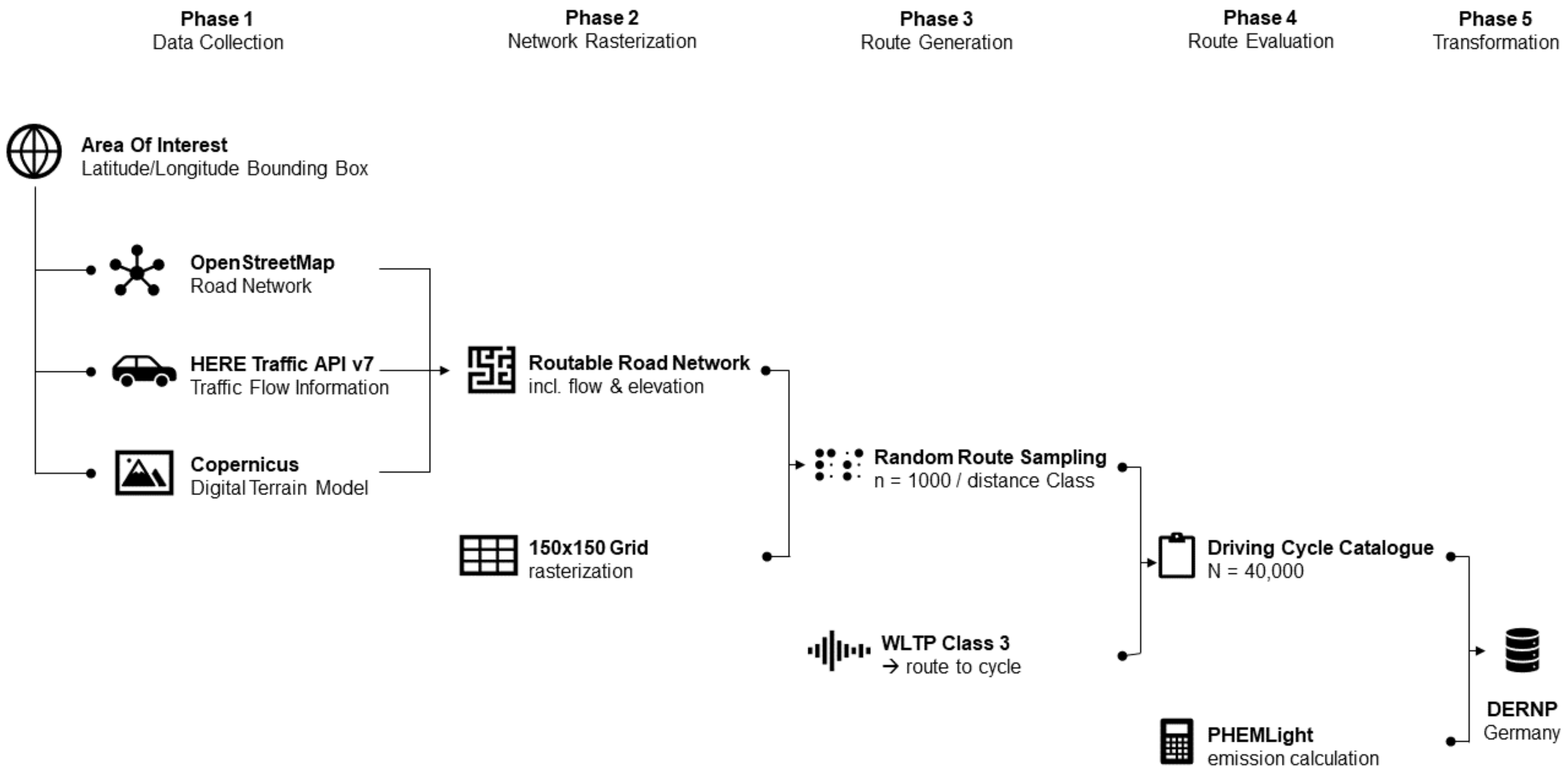
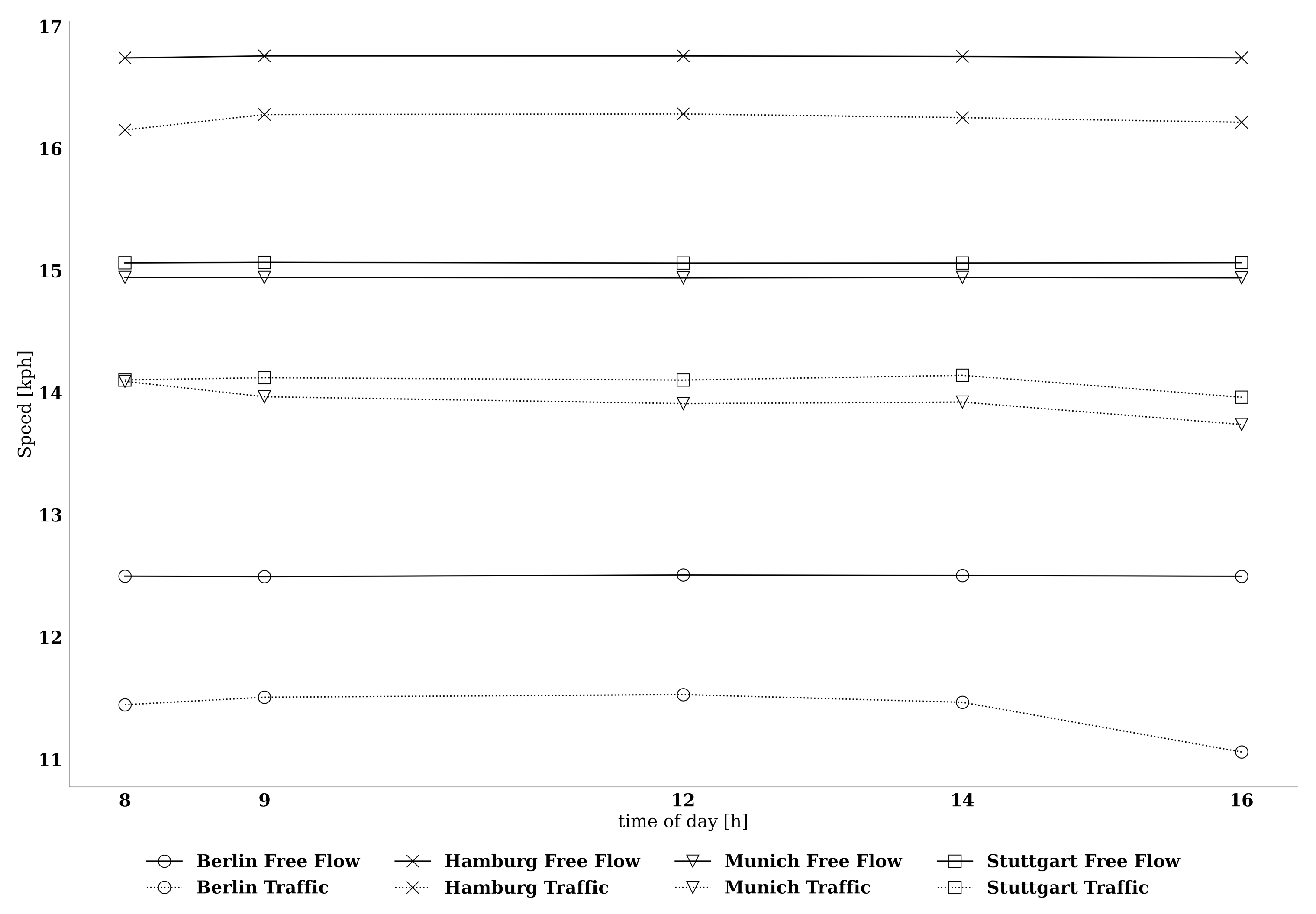
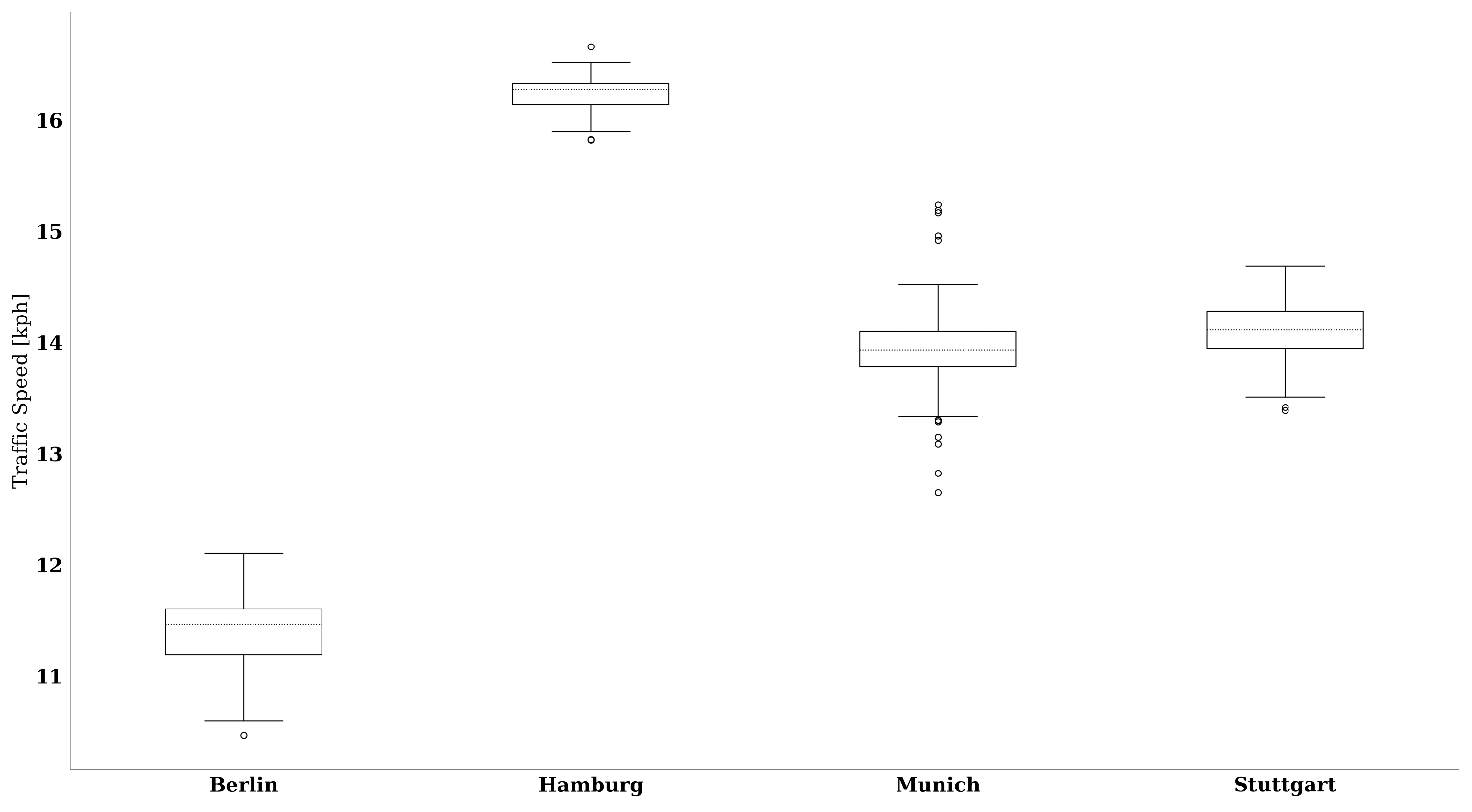
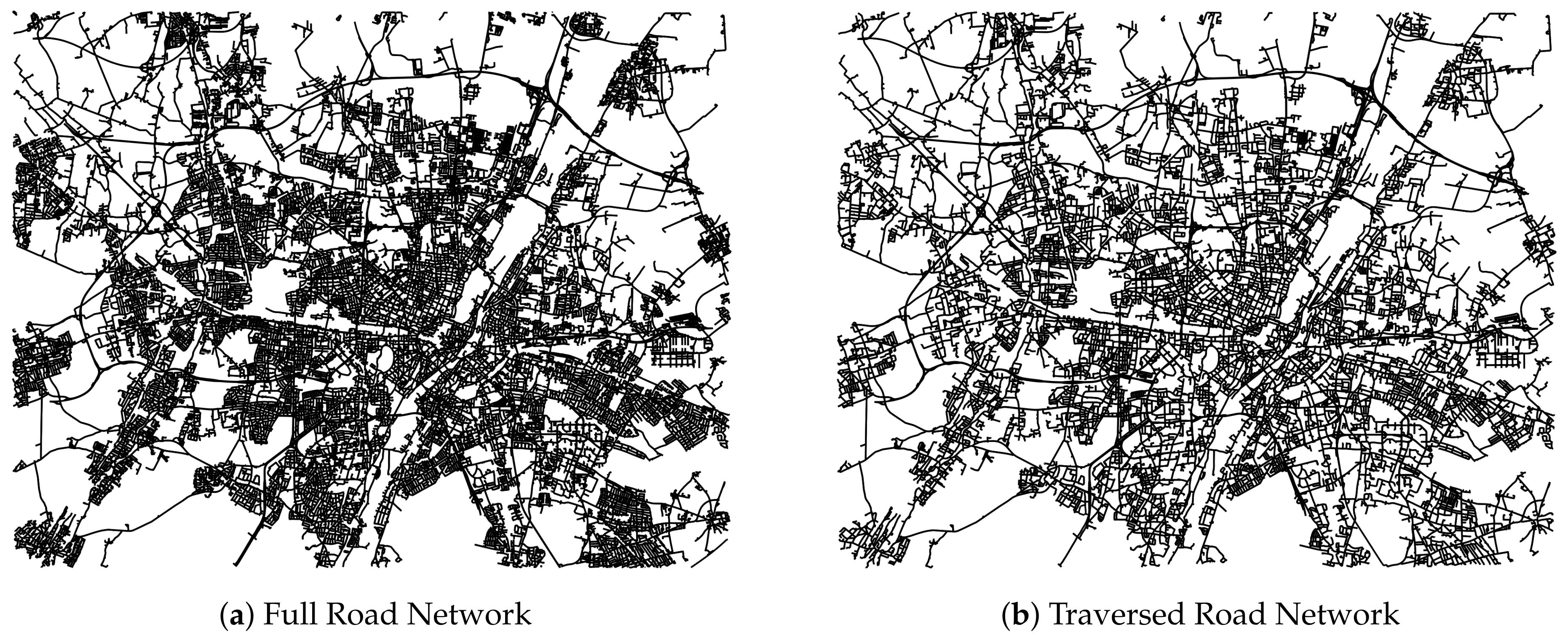
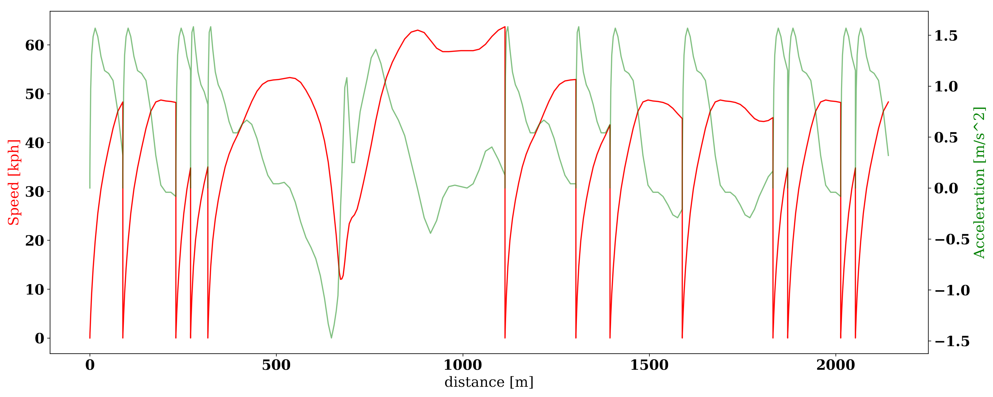
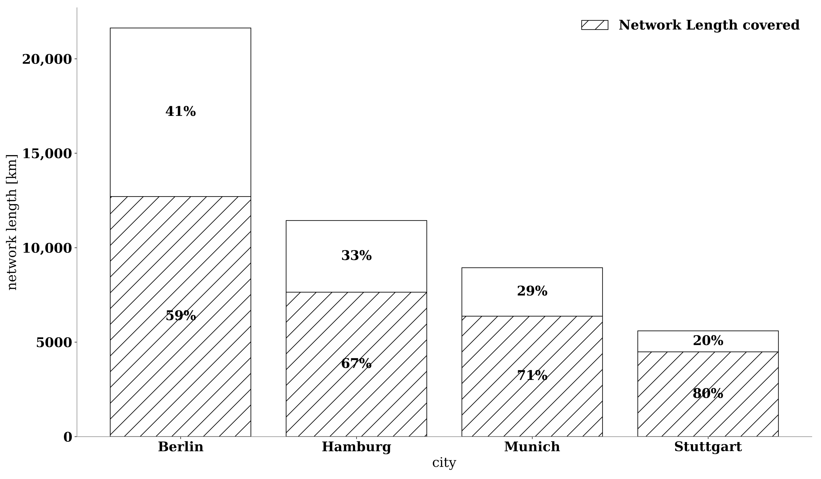
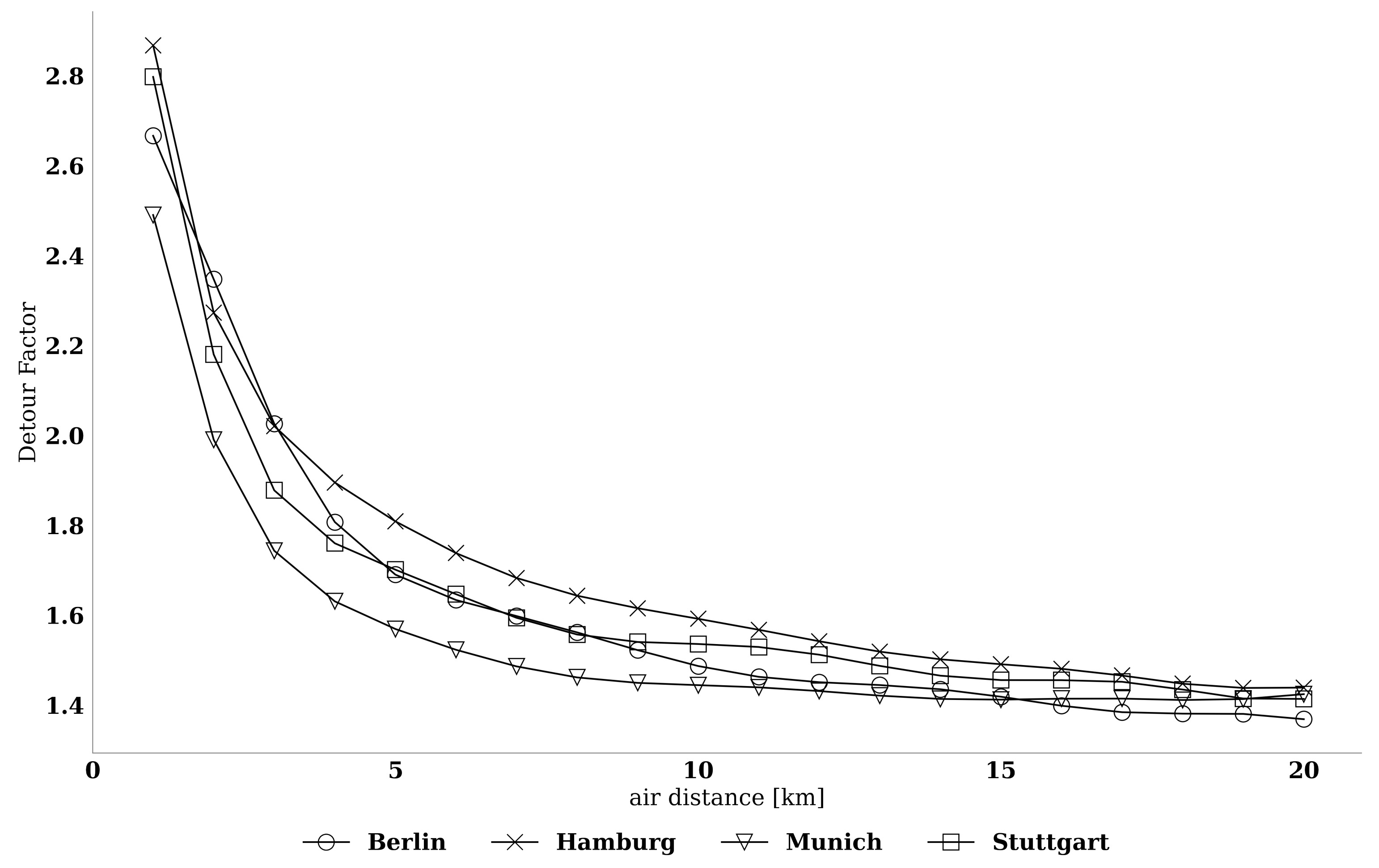
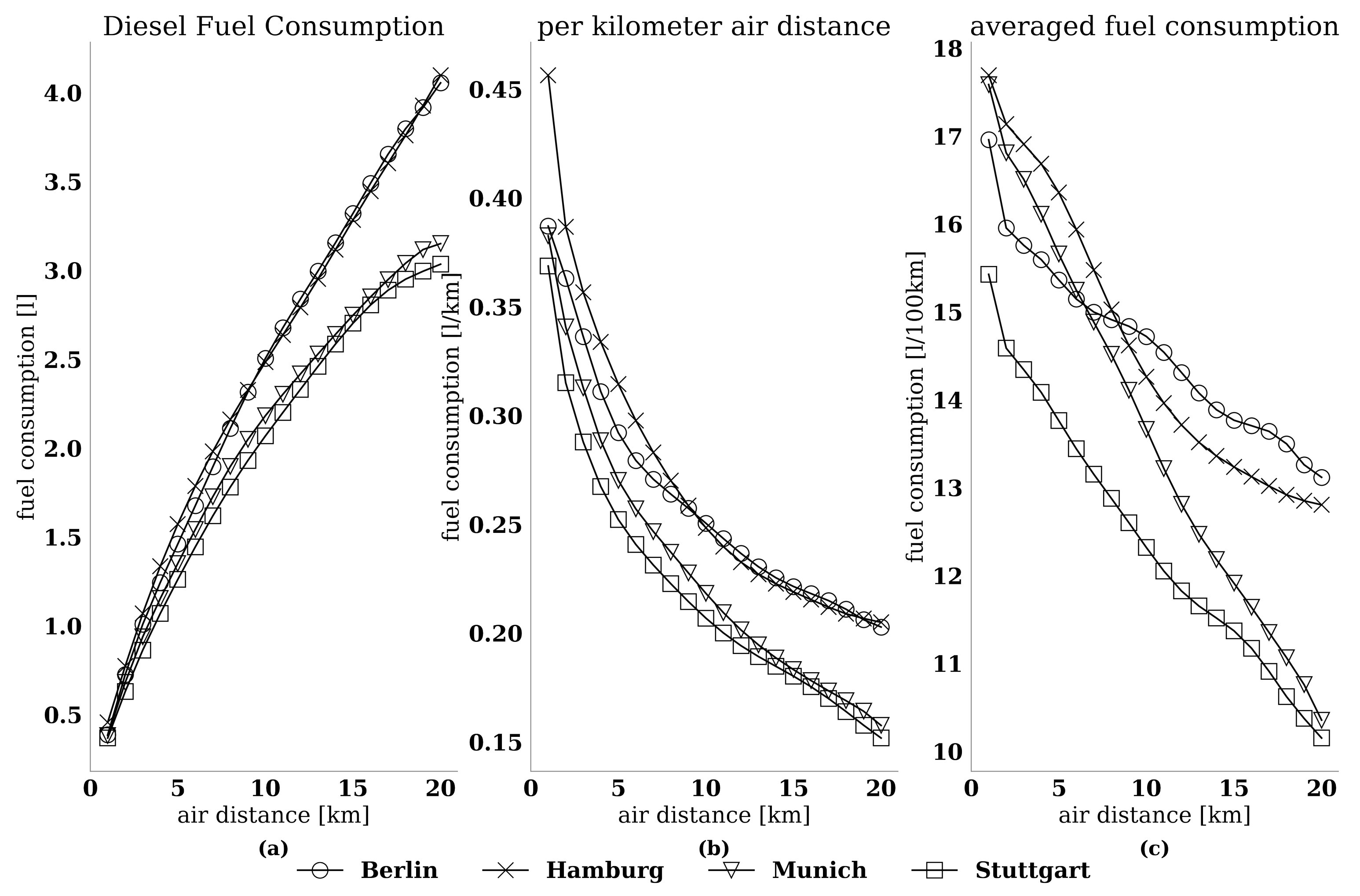
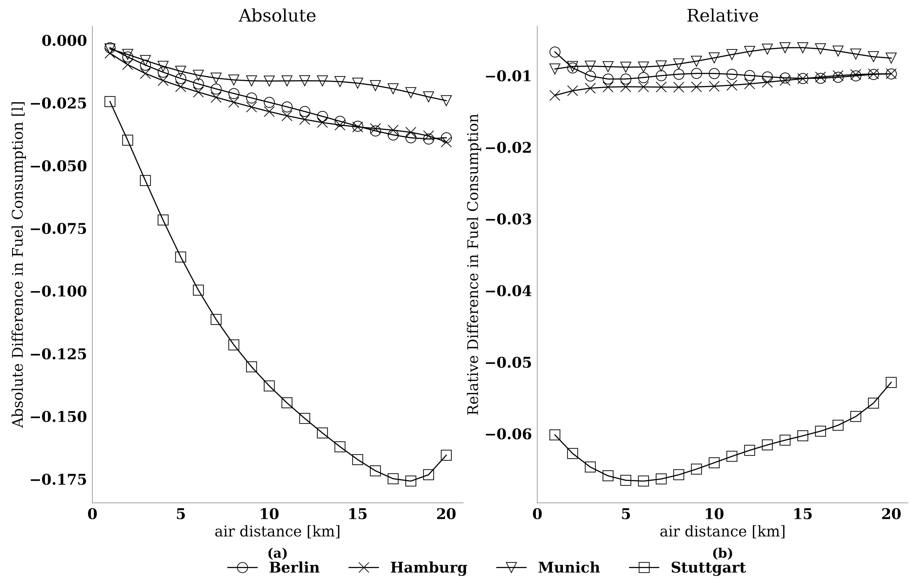
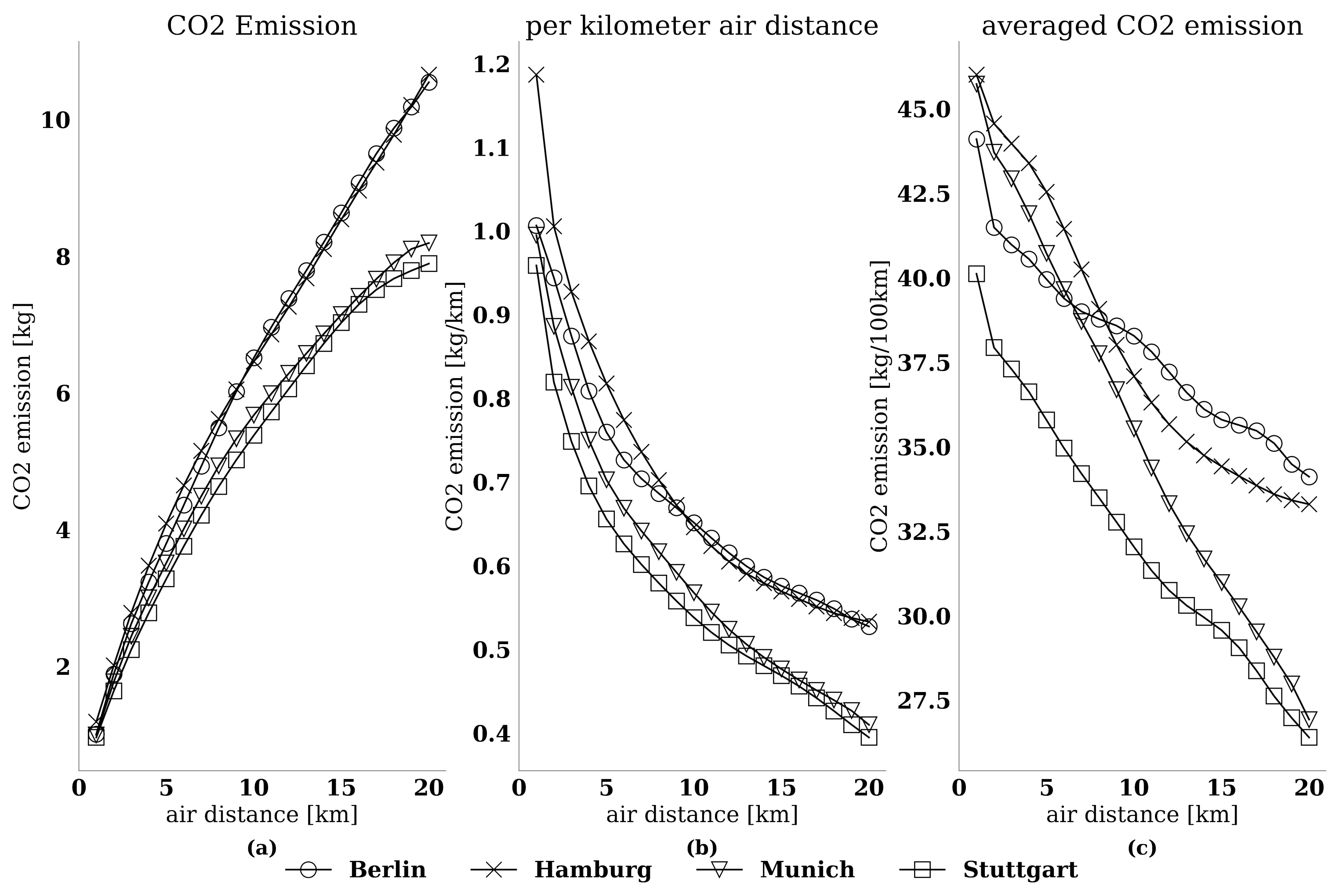
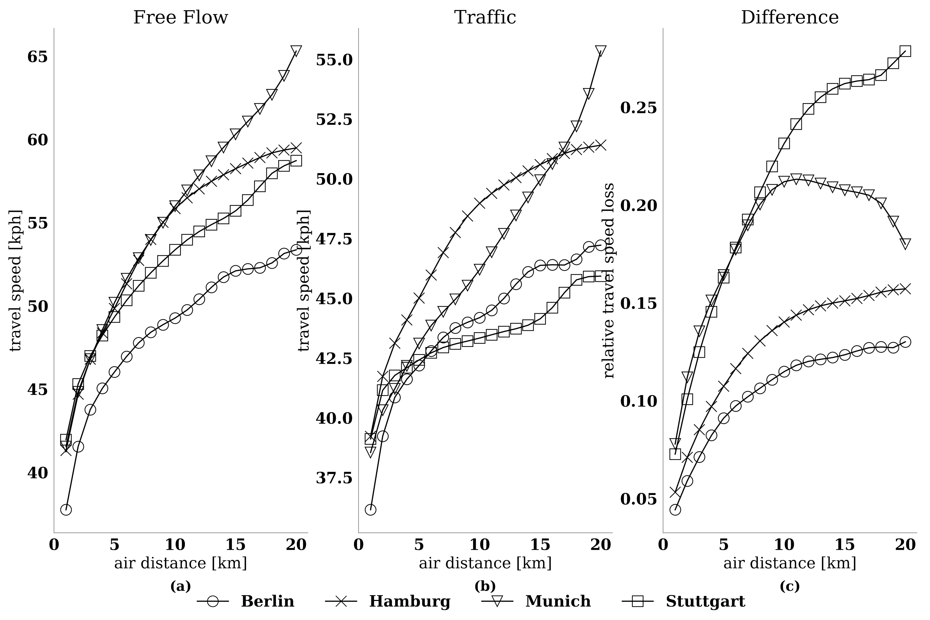
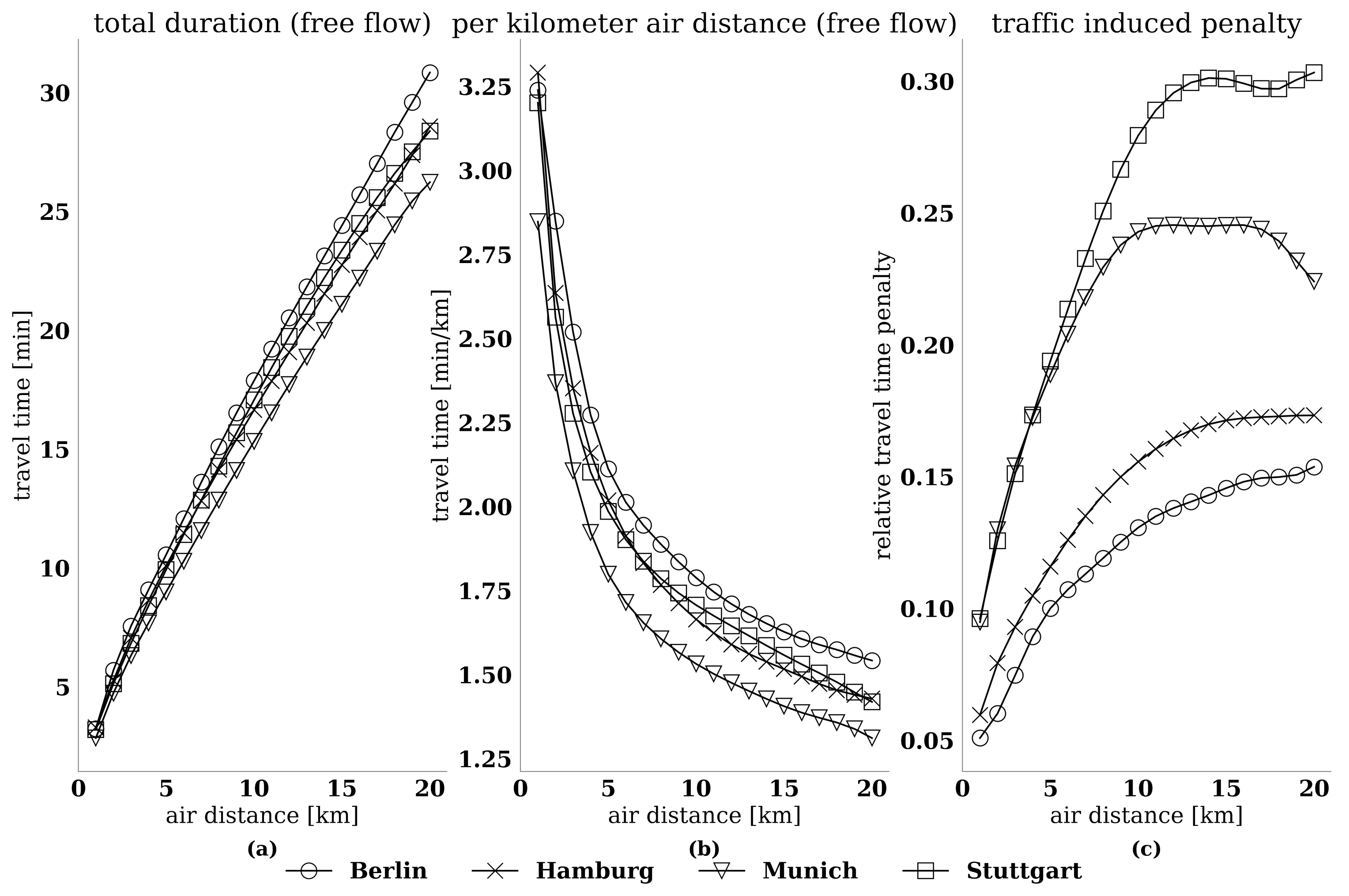
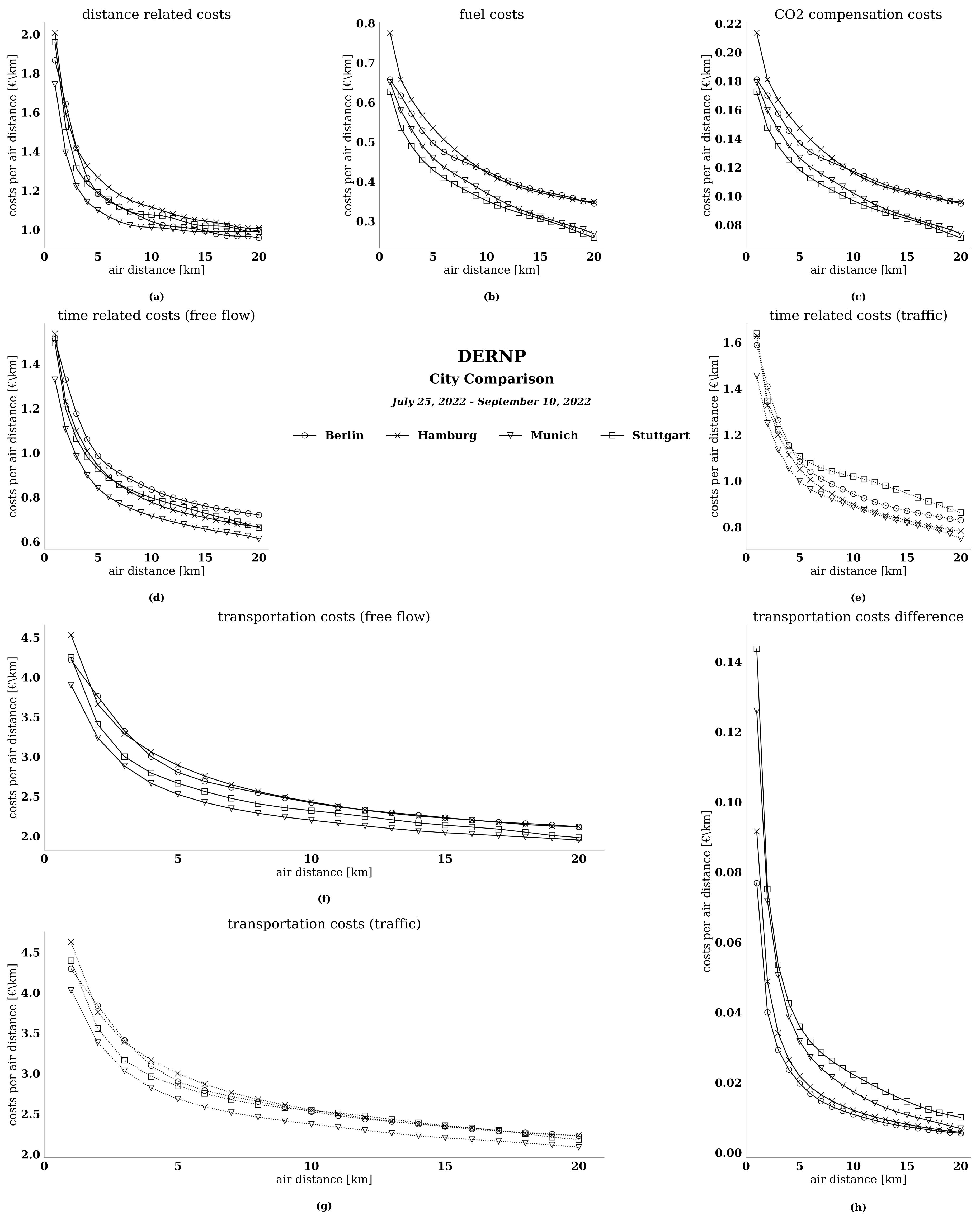
Table 1.
Description of Network Performance Factors included in DERNP.
| Variable | Description | Explanation |
|---|---|---|
| Air distance | The air distance from a start point to an end point | |
| Detour Factor regression | Continuous Detour Factor regression based on discrete measures | |
| Free flow velocity regression | Continuous free flow velocity regression based on discrete measures | |
| Traffic velocity regression | Continuous traffic velocity regression based on discrete measures | |
| Free flow travel time regression | Continuous free flow travel time regression based on discrete measures | |
| Traffic travel time regression | Continuous traffic traveltime regression based on discrete measures | |
| Fuel consumption regression | Continuous free flow fuel consumption regression based on discrete measures | |
| Avg. fuel consumption per 100 km regression | Continuous fuel consumption regression based on discrete measures | |
| CO2() | CO2 emission regression | Continuous CO2 emission regression based on discrete measures |
| CO2avg() | Avg. CO2 emission per 100 km regression | Continuous CO2 emission regression based on discrete measures |
Table 2.
Excerpt of the DERNP reference database for the top six largest German cities.
| City | Vehicle | Engine | Category | Factor | Unit | a | b | c | d | e | f | g | h | i | j | k | RMSE | ||
|---|---|---|---|---|---|---|---|---|---|---|---|---|---|---|---|---|---|---|---|
| Berlin | PKW | Diesel | EUR 4 | df | [-] | 0.5 | 20.5 | 1.940 × 10⁻¹⁰ | −1872 × 10−8 | 7.288 × 10⁻⁷ | −1.408 × 10⁻⁵ | 0.000 | 0.000 | −0.015 | 0.124 | −0.426 | 0.299 | 2.684 | 0.00 |
| Berlin | PKW | Diesel | EUR 4 | vf | [kph] | 0.5 | 20.5 | 4.197 × 10⁻⁹ | −4.754 × 10⁻⁷ | 2.285 × 10⁻⁵ | −0.001 | 0.010 | −0.098 | 0.600 | −2.076 | 3.068 | 2.615 | 33.630 | 0.03 |
| Berlin | PKW | Diesel | EUR 4 | vt | [kph] | 0.5 | 20.5 | 4.708 × 10⁻⁹ | −5.335 × 10⁻⁷ | 2.567 × 10⁻⁵ | −0.001 | 0.011 | −0.111 | 0.686 | −2.419 | 3.912 | 0.820 | 33.250 | 0.05 |
| Berlin | PKW | Diesel | EUR 4 | tf | [min] | 0.5 | 20.5 | 1.980 × 10⁻⁹ | −2.118 × 10⁻⁷ | 9.728 × 10⁻⁶ | −0.000 | 0.004 | −0.039 | 0.237 | −0.812 | 1.187 | 2.019 | 0.644 | 0.02 |
| Berlin | PKW | Diesel | EUR 4 | tt | [min] | 0.5 | 20.5 | 1.467 × 10⁻⁹ | −1.568 × 10⁻⁷ | 7.214 × 10⁻⁶ | −0.000 | 0.003 | −0.030 | 0.180 | −0.607 | 0.796 | 2.553 | 0.509 | 0.02 |
| Berlin | PKW | Diesel | EUR 4 | fc | [l] | 0.5 | 20.5 | 1.174 × 10⁻¹⁰ | −1.272 × 10⁻⁸ | 6.098 × 10⁻⁷ | −1.687 × 10⁻⁵ | 0.000 | −0.003 | 0.023 | −0.092 | 0.176 | 0.200 | 0.084 | 0.00 |
| Berlin | PKW | Diesel | EUR 4 | FC | [l/100 km] | 0.5 | 20.5 | 4.292 × 10⁻¹⁰ | −5.421 × 10⁻⁸ | 3.082 × 10⁻⁶ | −0.000 | 0.002 | −0.029 | 0.247 | −1.333 | 4.251 | −7.365 | 21.185 | 0.01 |
| Berlin | PKW | Diesel | EUR 4 | CO2 | [kg] | 0.5 | 20.5 | 3.052 × 10⁻¹⁰ | −3.308 × 10⁻⁸ | 1.586 × 10⁻⁶ | −4.386 × 10⁻⁵ | 0.001 | −0.008 | 0.059 | −0.240 | 0.457 | 0.521 | 0.217 | 0.00 |
| Berlin | PKW | Diesel | EUR 4 | CO2avg | [kg/100 km] | 0.5 | 20.5 | 1.116 × 10⁻⁹ | −1.410 × 10⁻⁷ | 8.014 × 10⁻⁶ | −0.000 | 0.006 | −0.074 | 0.642 | −3.466 | 11.055 | −19.151 | 55.090 | 0.04 |
| Hamburg | PKW | Diesel | EUR 4 | df | [-] | 0.5 | 20.5 | −1.792 × 10⁻¹⁰ | 1.714 × 10⁻⁸ | −6.673 × 10⁻⁷ | 1.310 × 10⁻⁵ | −0.000 | −0.000 | 0.014 | −0.143 | 0.719 | −1.947 | 4.226 | 0.00 |
| Hamburg | PKW | Diesel | EUR 4 | vf | [kph] | 0.5 | 20.5 | 1.712 × 10⁻⁹ | −1.816 × 10⁻⁷ | 8.242 × 10⁻⁶ | −0.000 | 0.003 | −0.029 | 0.143 | −0.252 | −0.907 | 6.434 | 35.914 | 0.05 |
| Hamburg | PKW | Diesel | EUR 4 | vt | [kph] | 0.5 | 20.5 | 1.130 × 10⁻⁹ | −1.214 × 10⁻⁷ | 5.575 × 10⁻⁶ | −0.000 | 0.002 | −0.019 | 0.088 | −0.071 | −1.138 | 5.572 | 34.787 | 0.07 |
| Hamburg | PKW | Diesel | EUR 4 | tf | [min] | 0.5 | 20.5 | −2.701 × 10⁻¹⁰ | 1.909 × 10⁻⁸ | −4.088 × 10⁻⁷ | −1.937 × 10⁻⁶ | 0.000 | −0.004 | 0.041 | −0.202 | 0.414 | 1.655 | 1.387 | 0.01 |
| Hamburg | PKW | Diesel | EUR 4 | tt | [min] | 0.5 | 20.5 | −3.435 × 10⁻¹⁰ | 2.495 × 10⁻⁸ | −5.875 × 10⁻⁷ | 3.964 × 10⁻⁷ | 0.000 | −0.005 | 0.045 | −0.222 | 0.479 | 1.780 | 1.411 | 0.01 |
| Hamburg | PKW | Diesel | EUR 4 | fc | [l] | 0.5 | 20.5 | −6.406 × 10⁻¹¹ | 5.459 × 10⁻⁹ | −1.846 × 10⁻⁷ | 3.011 × 10⁻⁶ | −1.953 × 10⁻⁵ | −9.656 × 10⁻⁵ | 0.003 | −0.019 | 0.049 | 0.266 | 0.158 | 0.00 |
| Hamburg | PKW | Diesel | EUR 4 | FC | [l/100 km] | 0.5 | 20.5 | −3.231 × 10⁻¹⁰ | 3.153 × 10⁻⁸ | −1.271 × 10⁻⁶ | 2.663 × 10⁻⁵ | −0.000 | 0.001 | 0.018 | −0.220 | 1.027 | −2.384 | 19.251 | 0.01 |
| Hamburg | PKW | Diesel | EUR 4 | CO2 | [kg] | 0.5 | 20.5 | −1.666 × 10⁻¹⁰ | 1.420 × 10⁻⁸ | −4.799 × 10⁻⁷ | 7.830 × 10⁻⁶ | −5.079 × 10⁻⁵ | −0.000 | 0.007 | −0.049 | 0.127 | 0.692 | 0.410 | 0.00 |
| Hamburg | PKW | Diesel | EUR 4 | CO2avg | [kg/100 km] | 0.5 | 20.5 | −8.403 × 10⁻¹⁰ | 8.199 × 10⁻⁸ | −3.305 × 10⁻⁶ | 6.925 × 10⁻⁵ | −0.001 | 0.002 | 0.048 | −0.571 | 2.671 | −6.199 | 50.061 | 0.06 |
| München | PKW | Diesel | EUR 4 | df | [-] | 0.5 | 20.5 | −3.203 × 10⁻¹⁰ | 3.440 × 10⁻⁸ | −1.579 × 10⁻⁶ | 4.032 × 10⁻⁵ | −0.001 | 0.006 | −0.033 | 0.085 | 0.060 | −0.929 | 3.302 | 0.00 |
| München | PKW | Diesel | EUR 4 | vf | [kph] | 0.5 | 20.5 | −2.995 × 10⁻⁹ | 3.313 × 10⁻⁷ | −1.593 × 10⁻⁵ | 0.000 | −0.007 | 0.084 | −0.610 | 2.840 | −8.105 | 14.696 | 32.648 | 0.12 |
| München | PKW | Diesel | EUR 4 | vt | [kph] | 0.5 | 20.5 | −4.217 × 10⁻⁹ | 4.607 × 10⁻⁷ | −2.185 × 10⁻⁵ | 0.001 | −0.010 | 0.109 | −0.765 | 3.388 | −8.926 | 13.501 | 31.246 | 0.12 |
| München | PKW | Diesel | EUR 4 | tf | [min] | 0.5 | 20.5 | 1.201 × 10⁻⁹ | −1.266 × 10⁻⁷ | 5.731 × 10⁻⁶ | −0.000 | 0.002 | −0.022 | 0.138 | −0.494 | 0.818 | 1.393 | 1.013 | 0.00 |
| München | PKW | Diesel | EUR 4 | tt | [min] | 0.5 | 20.5 | 1.424 × 10⁻⁹ | −1.503 × 10⁻⁷ | 6.846 × 10⁻⁶ | −0.000 | 0.003 | −0.028 | 0.179 | −0.668 | 1.237 | 1.237 | 1.159 | 0.01 |
| München | PKW | Diesel | EUR 4 | fc | [l] | 0.5 | 20.5 | 1.262 × 10⁻¹⁰ | −1.505 × 10⁻⁸ | 7.663 × 10⁻⁷ | −2.180 × 10⁻⁵ | 0.000 | −0.004 | 0.028 | −0.114 | 0.233 | 0.079 | 0.160 | 0.00 |
| München | PKW | Diesel | EUR 4 | FC | [l/100 km] | 0.5 | 20.5 | 1.622 × 10⁻⁹ | −1.901 × 10⁻⁷ | 9.611 × 10⁻⁶ | −0.000 | 0.005 | −0.055 | 0.401 | −1.830 | 4.919 | −7.311 | 21.459 | 0.02 |
| München | PKW | Diesel | EUR 4 | CO2 | [kg] | 0.5 | 20.5 | 3.283 × 10⁻¹⁰ | −3.912 × 10⁻⁸ | 1.993 × 10⁻⁶ | −5.668 × 10⁻⁵ | 0.001 | −0.011 | 0.073 | −0.296 | 0.606 | 0.205 | 0.416 | 0.00 |
| München | PKW | Diesel | EUR 4 | CO2avg | [kg/100 km] | 0.5 | 20.5 | 4.219 × 10⁻⁹ | −4.944 × 10⁻⁷ | 2.499 × 10⁻⁵ | −0.001 | 0.013 | −0.143 | 1.043 | −4.759 | 12.792 | −19.013 | 55.801 | 0.13 |
| Köln | PKW | Diesel | EUR 4 | df | [-] | 0.5 | 20.5 | 4.041 × 10⁻¹⁰ | −4.840 × 10⁻⁸ | 2.513 × 10⁻⁶ | −7.405 × 10⁻⁵ | 0.001 | −0.016 | 0.126 | −0.623 | 1.871 | −3.212 | 4.473 | 0.00 |
| Köln | PKW | Diesel | EUR 4 | vf | [kph] | 0.5 | 20.5 | −4.075 × 10⁻⁹ | 4.226 × 10⁻⁷ | −1.879 × 10⁻⁵ | 0.000 | −0.007 | 0.072 | −0.466 | 1.997 | −5.693 | 12.228 | 33.587 | 0.09 |
| Köln | PKW | Diesel | EUR 4 | vt | [kph] | 0.5 | 20.5 | −5.960 × 10⁻⁹ | 6.259 × 10⁻⁷ | −2.827 × 10⁻⁵ | 0.001 | −0.011 | 0.114 | −0.745 | 3.114 | −8.138 | 14.139 | 32.156 | 0.11 |
| Köln | PKW | Diesel | EUR 4 | tf | [min] | 0.5 | 20.5 | −7.929 × 10⁻¹⁰ | 7.798 × 10⁻⁸ | −3.219 × 10⁻⁶ | 7.206 × 10⁻⁵ | −0.001 | 0.007 | −0.028 | 0.038 | −0.035 | 1.991 | 1.148 | 0.01 |
| Köln | PKW | Diesel | EUR 4 | tt | [min] | 0.5 | 20.5 | −6.828 × 10⁻¹⁰ | 6.973 × 10⁻⁸ | −2.976 × 10⁻⁶ | 6.854 × 10⁻⁵ | −0.001 | 0.007 | −0.026 | 0.023 | 0.031 | 2.002 | 1.197 | 0.02 |
| Köln | PKW | Diesel | EUR 4 | fc | [l] | 0.5 | 20.5 | 3.781 × 10⁻¹¹ | −4.704 × 10⁻⁹ | 2.545 × 10⁻⁷ | −7.801 × 10⁻⁶ | 0.000 | −0.002 | 0.014 | −0.063 | 0.150 | 0.107 | 0.178 | 0.00 |
| Köln | PKW | Diesel | EUR 4 | FC | [l/100 km] | 0.5 | 20.5 | 3.692 × 10⁻⁹ | −4.036 × 10⁻⁷ | 1.903 × 10⁻⁵ | −0.001 | 0.008 | −0.089 | 0.615 | −2.677 | 6.995 | −10.279 | 21.893 | 0.01 |
| Köln | PKW | Diesel | EUR 4 | CO2 | [kg] | 0.5 | 20.5 | 9.833 × 10⁻¹¹ | −1.223 × 10⁻⁸ | 6.617 × 10⁻⁷ | −2.029 × 10⁻⁵ | 0.000 | −0.005 | 0.036 | −0.165 | 0.389 | 0.279 | 0.462 | 0.00 |
| Köln | PKW | Diesel | EUR 4 | CO2avg | [kg/100 km] | 0.5 | 20.5 | 9.600 × 10⁻⁹ | −1.050 × 10⁻⁶ | 4.949 × 10⁻⁵ | −0.001 | 0.022 | −0.232 | 1.599 | −6.961 | 18.191 | −26.730 | 56.931 | 0.07 |
| Frankfurt am Main | PKW | Diesel | EUR 4 | df | [-] | 0.5 | 20.5 | 2.676 × 10⁻⁹ | −2.965 × 10⁻⁷ | 1.419 × 10⁻⁵ | −0.000 | 0.006 | −0.070 | 0.489 | −2.167 | 5.774 | −8.516 | 7.485 | 0.00 |
| Frankfurt am Main | PKW | Diesel | EUR 4 | vf | [kph] | 0.5 | 20.5 | 6.967 × 10⁻⁹ | −7.318 × 10⁻⁷ | 3.299 × 10⁻⁵ | −0.001 | 0.013 | −0.129 | 0.796 | −2.904 | 5.212 | 0.590 | 39.073 | 0.09 |
| Frankfurt am Main | PKW | Diesel | EUR 4 | vt | [kph] | 0.5 | 20.5 | 6.223 × 10⁻⁹ | −6.530 × 10⁻⁷ | 2.944 × 10⁻⁵ | −0.001 | 0.012 | −0.115 | 0.715 | −2.594 | 4.583 | 0.373 | 37.502 | 0.15 |
| Frankfurt am Main | PKW | Diesel | EUR 4 | tf | [min] | 0.5 | 20.5 | −1.173 × 10⁻⁹ | 1.201 × 10⁻⁷ | −5.301 × 10⁻⁶ | 0.000 | −0.002 | 0.021 | −0.143 | 0.623 | −1.716 | 4.126 | 0.440 | 0.01 |
| Frankfurt am Main | PKW | Diesel | EUR 4 | tt | [min] | 0.5 | 20.5 | −1.423 × 10⁻⁹ | 1.447 × 10⁻⁷ | −6.337 × 10⁻⁶ | 0.000 | −0.002 | 0.024 | −0.157 | 0.659 | −1.721 | 4.217 | 0.552 | 0.01 |
| Frankfurt am Main | PKW | Diesel | EUR 4 | fc | [l] | 0.5 | 20.5 | −2.836 × 10⁻¹⁰ | 2.938 × 10⁻⁸ | −1.306 × 10⁻⁶ | 3.262 × 10⁻⁵ | −0.001 | 0.005 | −0.032 | 0.125 | −0.296 | 0.585 | 0.021 | 0.00 |
| Frankfurt am Main | PKW | Diesel | EUR 4 | FC | [l/100 km] | 0.5 | 20.5 | −4.341 × 10⁻¹⁰ | 4.092 × 10⁻⁸ | −1.584 × 10⁻⁶ | 3.168 × 10⁻⁵ | −0.000 | 0.001 | 0.021 | −0.257 | 1.355 | −3.991 | 18.952 | 0.01 |
| Frankfurt am Main | PKW | Diesel | EUR 4 | CO2 | [kg] | 0.5 | 20.5 | −7.374 × 10⁻¹⁰ | 7.639 × 10⁻⁸ | −3.396 × 10⁻⁶ | 8.483 × 10⁻⁵ | −0.001 | 0.013 | −0.082 | 0.324 | −0.770 | 1.521 | 0.053 | 0.00 |
| Frankfurt am Main | PKW | Diesel | EUR 4 | CO2avg | [kg/100 km] | 0.5 | 20.5 | −1.129 × 10⁻⁹ | 1.064 × 10⁻⁷ | −4.118 × 10⁻⁶ | 8.239 × 10⁻⁵ | −0.001 | 0.002 | 0.055 | −0.669 | 3.524 | −10.379 | 49.282 | 0.05 |
| Stuttgart | PKW | Diesel | EUR 4 | df | [-] | 0.5 | 20.5 | −6.547 × 10⁻¹⁰ | 7.186 × 10⁻⁸ | −3.378 × 10⁻⁶ | 8.867 × 10⁻⁵ | −0.001 | 0.014 | −0.087 | 0.291 | −0.349 | −0.666 | 3.596 | 0.00 |
| Stuttgart | PKW | Diesel | EUR 4 | vf | [kph] | 0.5 | 20.5 | 1.109 × 10⁻⁹ | −8.093 × 10⁻⁸ | 1.860 × 10⁻⁶ | 4.439 × 10⁻⁶ | −0.001 | 0.022 | −0.233 | 1.465 | −5.433 | 12.278 | 33.859 | 0.06 |
| Stuttgart | PKW | Diesel | EUR 4 | vt | [kph] | 0.5 | 20.5 | 1.706 × 10⁻⁹ | −1.436 × 10⁻⁷ | 4.676 × 10⁻⁶ | −6.634 × 10⁻⁵ | 7.573 × 10⁻⁵ | 0.011 | −0.168 | 1.208 | −4.713 | 9.908 | 32.866 | 0.08 |
| Stuttgart | PKW | Diesel | EUR 4 | tf | [min] | 0.5 | 20.5 | 5.500 × 10⁻¹⁰ | −5.351 × 10⁻⁸ | 2.211 × 10⁻⁶ | −5.058 × 10⁻⁵ | 0.001 | −0.006 | 0.030 | −0.068 | −0.078 | 2.336 | 0.987 | 0.01 |
| Stuttgart | PKW | Diesel | EUR 4 | tt | [min] | 0.5 | 20.5 | 2.543 × 10⁻¹⁰ | −2.566 × 10⁻⁸ | 1.105 × 10⁻⁶ | −2.659 × 10⁻⁵ | 0.000 | −0.004 | 0.020 | −0.050 | −0.055 | 2.567 | 1.031 | 0.01 |
| Stuttgart | PKW | Diesel | EUR 4 | fc | [l] | 0.5 | 20.5 | 9.131 × 10⁻¹¹ | −1.052 × 10⁻⁸ | 5.215 × 10⁻⁷ | −1.448 × 10⁻⁵ | 0.000 | −0.003 | 0.018 | −0.070 | 0.141 | 0.132 | 0.151 | 0.00 |
| Stuttgart | PKW | Diesel | EUR 4 | FC | [l/100 km] | 0.5 | 20.5 | 5.594 × 10⁻¹⁰ | −7.621 × 10⁻⁸ | 4.361 × 10⁻⁶ | −0.000 | 0.003 | −0.033 | 0.263 | −1.313 | 3.892 | −6.399 | 19.014 | 0.01 |
| Stuttgart | PKW | Diesel | EUR 4 | CO2 | [kg] | 0.5 | 20.5 | 2.374 × 10⁻¹⁰ | −2.736 × 10⁻⁸ | 1.356 × 10⁻⁶ | −3.766 × 10⁻⁵ | 0.001 | −0.007 | 0.046 | −0.182 | 0.366 | 0.344 | 0.391 | 0.00 |
| Stuttgart | PKW | Diesel | EUR 4 | CO2avg | [kg/100 km] | 0.5 | 20.5 | 1.455 × 10⁻⁹ | −1.982 × 10⁻⁷ | 1.134 × 10⁻⁵ | −0.000 | 0.007 | −0.086 | 0.685 | −3.414 | 10.121 | −16.639 | 49.445 | 0.07 |
Disclaimer/Publisher’s Note: The statements, opinions and data contained in all publications are solely those of the individual author(s) and contributor(s) and not of MDPI and/or the editor(s). MDPI and/or the editor(s) disclaim responsibility for any injury to people or property resulting from any ideas, methods, instructions or products referred to in the content. |
© 2022 by the authors. Licensee MDPI, Basel, Switzerland. This article is an open access article distributed under the terms and conditions of the Creative Commons Attribution (CC BY) license (https://creativecommons.org/licenses/by/4.0/).
Share and Cite
MDPI and ACS Style
Kunkler, J.; Kellner, F. Sustainable City Evaluation Using the Database for Estimation of Road Network Performance. Sustainability 2023, 15, 733. https://doi.org/10.3390/su15010733
AMA Style
Kunkler J, Kellner F. Sustainable City Evaluation Using the Database for Estimation of Road Network Performance. Sustainability. 2023; 15(1):733. https://doi.org/10.3390/su15010733
Chicago/Turabian StyleKunkler, Jan, and Florian Kellner. 2023. "Sustainable City Evaluation Using the Database for Estimation of Road Network Performance" Sustainability 15, no. 1: 733. https://doi.org/10.3390/su15010733
Note that from the first issue of 2016, this journal uses article numbers instead of page numbers. See further details here.