A Machine Learning-Based Approach to Estimate Energy Flows of the Mangrove Forest: The Case of Panama Bay

Abstract

Two models were developed to simulate energy flows in a mangrove area of A. germinans and A. bicolor in the Bay of Panama, considering the importance of these areas in CO₂ fixation. The first model (black box) consisted of the use of artificial neural networks for estimation, using meteorological data and energy flows calculated by the Eddy Covariance method for model training. The second model (grey box) used the RC circuit theory, considering a non-steady state model for the flow of water from the ground to the atmosphere. A methodology was developed to reduce the uncertainty of the data collected by the sensors in the field. The black box model managed to predict the fluxes of latent heat (R² > 0.91), sensible heat (R² > 0.86), CO₂ (R² > 0.88), and the potential of water in the air (R² > 0.88) satisfactorily, while the grey box model generated R² values of 0.43 and 0.37, indicating that it requires further analysis regarding the structuring of the equations and parameters used. The application of the methodology to filter the data improved the effectiveness of the model during the predictions, reducing the computational capacity necessary for the resolution of the iterations.

1. Introduction

The increase in the planet’s temperature, attributed to the production of greenhouse gases, has increased the interest in improving industrialization practices and finding techniques that allow for mitigating CO₂ concentrations in the atmosphere [1]. Mangroves can store more carbon per hectare, compared to tropical forests; they are also essential to maintain terrestrial and marine fauna [2,3,4]. In addition, these mangrove coastal areas can retain pollutants such as heavy metals in the tributaries, as well as reduce the effects caused by strong waves, floods, and even cyclonic winds, thanks to the presence of abundant aerial biomass that manages to dissipate the energy coming from of the outside [4,5,6,7,8,9,10,11]. Despite the importance of mangrove areas, they are affected worldwide due to bad human practices through fishing, logging, and the construction of spaces for tourism, interventions that modify the concentrations of nutrients and the hydroperiod of the ecosystem [12,13].

We can find multiple studies that analyze the energy exchange in coastal areas, as well as the hydrological modifications they suffer due to the intervention of the human being [14,15,16,17]. Such studies allow us to understand the dynamics of these ecosystems, evidencing the significant contribution to the capture and fixation of CO₂ from the atmosphere through trees and sediment transport, monitoring the resources available to the ecosystem to analyze the productivity and efficiency in the transfer and dissipation of energy [18].

Sensible heat flux (H), latent heat flux (LE), and ground heat flux (G) are the main ways in which the forest processes the radiation it receives from the sun. These energy flows condition the productivity of forests, which is why there are multiple strategies to determine them [19]. The Eddy Covariance (EC) method is one of those used to determine flows, where variables such as CO₂/H₂O concentrations, wind speed, and direction are recorded, considering the exchange between the forest and the atmosphere due to the turbulent flow of the wind [20]. This method requires the installation of sophisticated measurement equipment to record meteorological variables, which translates into a considerable initial investment. Therefore, many authors choose to estimate LE and H through simulations [19]. Other methods used include remote sensing, the Penman–Monteith equation, the Shuttleworth and Wallace method, and artificial neural networks [21,22].

One of the main advantages of remote sensing lies in the ability to monitor large areas based on satellite images that are recorded for the treatment and identification of vegetation indices. However, the most direct way to measure evapotranspiration is related to the EC method [23]. Multiple crops were analyzed by [24] to determine evapotranspiration using remote sensing, obtaining a coefficient of determination R² of 0.74 when the data were compared with measurements obtained by Bowen’s relationship. In the case of [25], an estimate of the evapotranspiration of a vineyard was made, obtaining an R² of 0.63 when comparing remote sensing with the EC methodology.

Artificial neural networks allow complex data processing, finding patterns between input and output variables, and allowing the prediction of behaviors of interest with much more accuracy than the aforementioned models [19]. This method has been used by multiple authors to estimate LE and H in different ecosystems around the world, but it should be noted that the configuration of these networks is often based on trial and error [26,27,28,29,30,31,32,33].

If more specific parameters of the forest are known, such as the water conditions of the tree, respiration, and factors that intervene during the photosynthesis process, it is possible to use methods that can predict the exchange between the forest and the atmosphere, such as soil-plant-atmosphere-continuum (SPAC) [34], where the flow of water in a non-steady state can be considered, to structure an analogy of electrical systems such as RC or RCL circuits such as those developed by [35,36,37,38,39,40,41]. The work developed by [42] considered a steady state flow; later [43] questioned these assumptions because it is far from the reality of the process, recommending the use of non-steady states in the plants. Continuing the focus on trees, there is the work of [44] where multiple allometric equations have been presented that attempt to estimate growth rates and carbon fixed in their biomass.

The objective of the study is to verify the effectiveness of artificial neural networks to predict LE, H, CO₂ flux (FC), and the potential of water in the air in mangrove ecosystems (Black box model), as well as to propose a methodology to determine the parameters that arise when using an RC circuit to estimate climatic variables within the ecosystem through state space representation (Grey box model). Because there are values for the latent heat and the potential of water in the air, the use of the cohesion-tension model is proposed to estimate the value of the resistances of the system, referring to the species that coexist in the area. The hypothesis for the use of this model (grey box) is that it may be possible to know the hydrological properties of the trees that make up the forest, using the records of latent heat and water potential generated by sensors installed in the area.

2. Materials and Methods

2.1. Artificial Intelligence

Artificial intelligence refers to the possibility that a machine can have to imitate the cognitive abilities of the human brain, being used in branches such as psychology, medicine, and statistics, among others [45]. Within artificial intelligence is machine learning, where its algorithms collect information on the selected database, making decisions based on patterns that were identified during the training process. A model is said to be learning if their performance on tasks, as measured by a performance benchmark, improves with experience assigned during training. The training process is realized through a training dataset, a collection of data points used to minimize the error between the predicted and real output, as established by the dataset. While the training process inevitably minimizes the training error, the goal of the optimization is to minimize the error in an unseen dataset, called the testing set. A model capable of performing acceptably in a testing dataset is said to have a good generalization capacity. Both training and testing or generalization errors vary with the characteristics of the training dataset, which include its size (number of examples), quality, and comprehension of the system’s dynamic behavior [46,47].

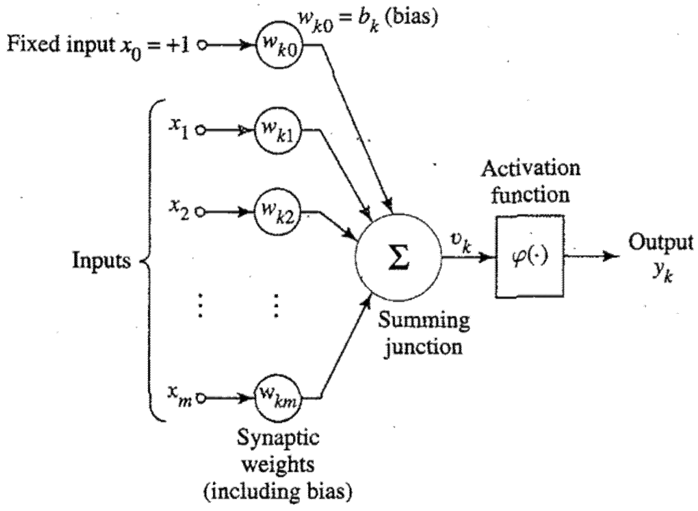
A subset of machine learning is artificial neural networks, models that consist of interconnected processing units called neurons. These interconnections allow to store knowledge acquired by the model during the learning process. The neural network seeks to define the function expressed in (1), where the parameters ($\theta$) identified as optimal during the training process are processed together with the inputs $(x)$ to obtain the output $(y)$ [47,48].

$$y=f(x; \theta )$$

(1)

A neuron is the fundamental processing unit in a neural network. The block diagram in Figure 1 shows the model of a neuron. The main elements of a neuron are:

• A set of synapses: each input “$x_j$” corresponding to a neuron “k” is multiplied by a weight “$w_{kj}$” which represents a parameter optimized by the machine learning algorithm.
• A summation process to add the “m” number of inputs multiplied by their weights.
• The activation function $\phi (v_k)$ that will determine the output of the neuron.

The respective equations for the process carried out by the neurons are shown in (2) and (3).

$$v_k={\displaystyle \sum }_{j=0}^m{w}_{kj}{x}_j$$

(2)

$$y_k=\phi (v_k)$$

(3)

2.2. Non-Steady State Model

The flow of water in trees can be explained by the cohesion-tension theory, which considers that the difference in pressure between the soil and the atmosphere allows the flow of water to rise through the xylem to be used within their biological processes such as respiration and photosynthesis [41]. Being considered a hydraulic system, the medium could generate some resistance to the passage of the fluid, which is why the hydraulic conductances (or their inverse, the resistances) are considered, as well as the storage of water in the different parts of the tree. These considerations allow for obtaining results that are much closer to the real conditions of the analyzed process [43].

Considering the net assimilation of CO₂, the work of [49] is observed, where he presents a model that involves stomatal conductance ($g_s$):

$$g_s=\frac{1.6 A}{C_s-C_i}$$

(4)

where $C_s$ is the concentration of CO₂ in the environment, $C_i$ is the concentration of CO₂ in the stomatal cavity, and A the net assimilation of CO₂ $({\mathsf{\mu }\mathrm{mol}\mathrm{m}}^{-2}{\mathrm{s}}^{-1})$ determined by (5):

$$A=((A_m+R_d)[1-e^{ \frac{-\epsilon I_a F_c}{A_m+R_d}} ]-R_d)F_{co2}$$

(5)

where $A_m$ is the net assimilation as a function of CO₂ $({\mathrm{mg}\mathrm{m}}^{-2}{\mathrm{s}}^{-1})$, $R_d$ is leaf respiration $({\mathrm{mg}\mathrm{m}}^{-2}{\mathrm{s}}^{-1})$, $I_a$ photosynthetic active radiation (PAR) reaching the $({\mathsf{\mu }\mathrm{mol}\mathrm{m}}^{-2}{\mathrm{s}}^{-1})$, ε is the initial quantum use efficiency $(\mathrm{mg} \mathrm{C}{\mathrm{O}}_2 {[ \mathrm{J} \mathrm{PAR}]}^{-1})$, $F_c$ is a conversion factor between PAR and its association with energy: $F_c=0.22 \mathrm{J} \mathrm{PAR} {\mathsf{\mu }\mathrm{mol}}^{-1}$ according to the ratio of 1 mol of photons $\equiv 0.22 \mathrm{MJ} \mathrm{PAR}$. $F_{co2}$ is a conversion between the mass unit and molar unit of CO₂ (22.727 $\mathsf{\mu }\mathrm{mol}$ CO₂ [g $\mathrm{C}{\mathrm{O}}_2{]}^{-1}$). This methodology was used in [49] because they had enough information on the type of species analyzed, collecting information in the study area and complementing with works developed by other authors.

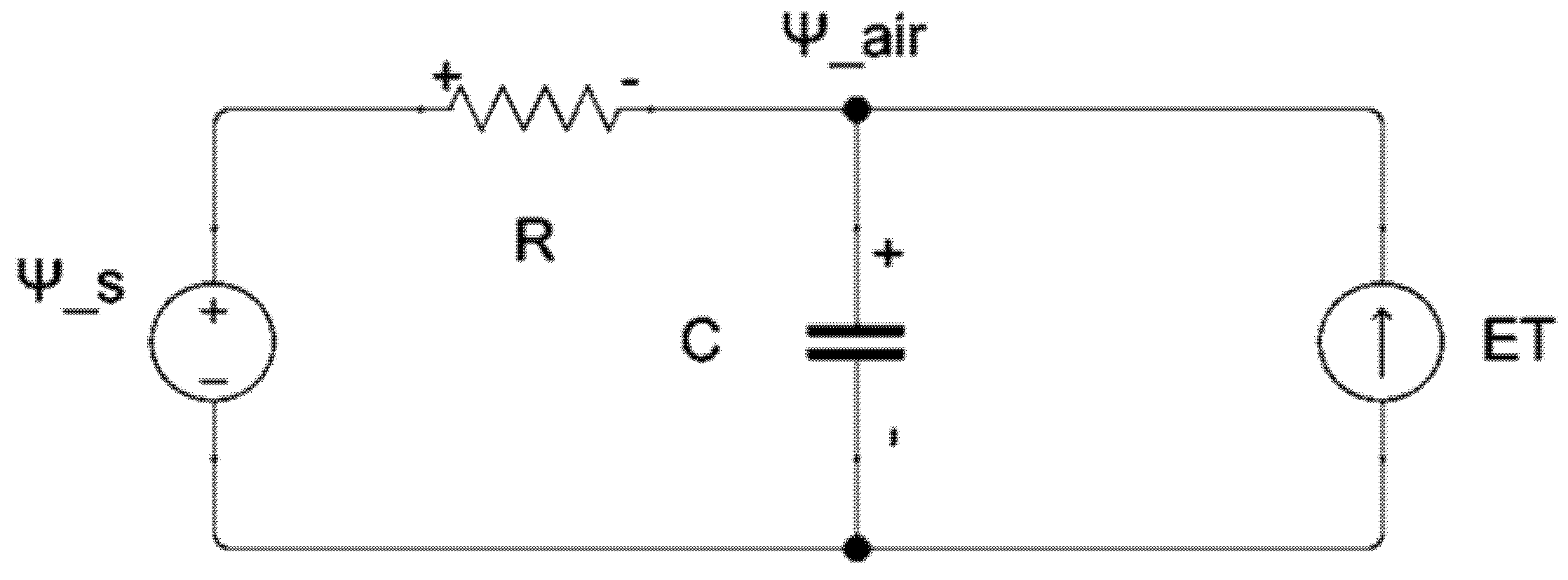
The hydraulic system can be represented by the analogy of Ohm’s law and it is used to determine the transpiration of trees or meteorological conditions such as the potential of water in the air [50]. Detailed explanations can be found in the works of Tyree and Ewers [42] and Kumagai [43]. Figure 2 shows a representative scheme of the analogy, including the potential of water in the air (${\mathsf{\Psi }}_{\mathrm{air}}$) and the ground (${\mathsf{\Psi }}_{\mathrm{s}}$), the evapotranspiration (ET), the hydric resistance (R), and the water storage (C) equivalents of the system.

Analyzing Figure 2, it is possible to extract an equation through a flow balance, shown in (6), where the known variables would be ${\mathsf{\Psi }}_{\mathrm{air}}$ determined by (7) [50] and ET obtained by the (EC) method.

$$\frac{{\mathsf{\Psi }}_{\mathrm{s}}-{\mathsf{\Psi }}_{\mathrm{air}}}{\mathrm{R}}+\mathrm{ET}=\mathrm{C}\frac{{\mathrm{d}\mathsf{\Psi }}_{\mathrm{air}}}{\mathrm{dt}}$$

(6)

$${\mathsf{\Psi }}_{\mathrm{air}}=\frac{\mathrm{RT}}{{\mathrm{V}}_{\mathrm{w}}}\ln (\mathrm{RH})$$

(7)

where, ${\mathrm{V}}_{\mathrm{w}}$ represents the partial molar volume of water (18.05 × 10⁻⁶ ${\mathrm{m}}^3/\mathrm{mol}$), T (K) the air temperature at 30.3 m, R the constant for ideal gases (8.31 $\mathrm{Pa} {\mathrm{m}}^3/\mathrm{mol}$ K), and RH the relative humidity. For the development of (6), it is possible to use a state space representation shown in (8).

$$\left[\frac{{\mathrm{d}\mathsf{\Psi }}_{\mathrm{air}}}{\mathrm{dt}}\right]=\left[\frac{1}{\mathrm{CR}}\left(\mathrm{G}-1\right)\right]\left[{\mathsf{\Psi }}_{\mathrm{air}}\right]+\left[\frac{1}{\mathrm{C}}\right]\left[\mathrm{ET}\right]$$

(8)

The variable G is a representation of the proportionality that must exist between ${\mathsf{\Psi }}_{\mathrm{air}}$ and ${\mathsf{\Psi }}_{\mathrm{s}}$ (${\mathsf{\Psi }}_{\mathrm{s}}$ = G ∗ ${\mathsf{\Psi }}_{\mathrm{air}}$), because in practice the determination of ${\mathsf{\Psi }}_{\mathrm{s}}$ is based on the measurement of the water potential in the leaves before dawn [51]. Once the state space representation is obtained, we proceed to use the identification process and optimization functions such as “idgrey” to enter the matrix and “greyest” for the solution through the method of least squares to minimize the error between the estimated and measured variables in the software MATLAB (version 2020b, 9.9.0.1467703) [52].

2.3. Site Information

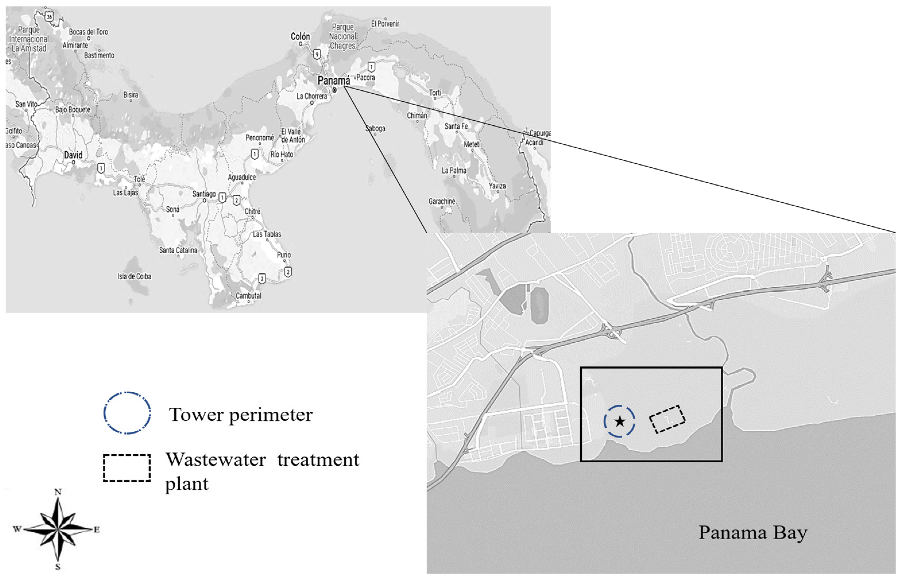
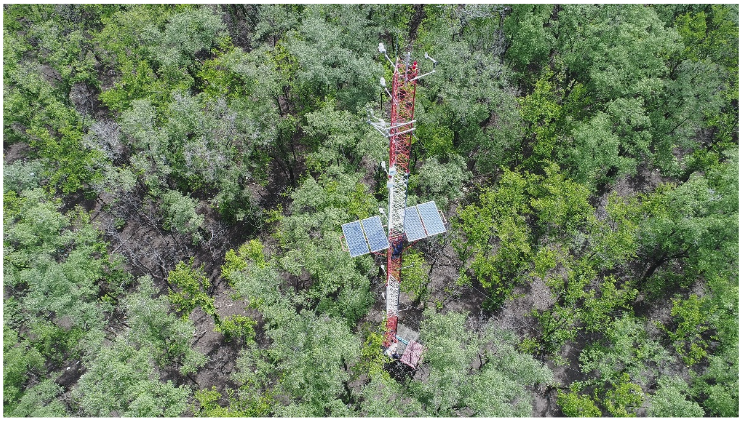
The experimental site (9°00′51.82″ N 79°27′10.60″ W) is located in a mangrove forest in the Bay of Panama (Figure 3), within the Juan Díaz neighborhood with an average temperature of 27 °C per year. Among the species that can be found close to the study area are Rhizophora mangle, Laguncularia racemosa, Avicennia germinans, and Avicennia bicolor, the last two species being present in the study area [53]. This area was selected due to the presence of a 30.3 m flow measurement tower (Figure 4) with multiple sensors (

Table 1. Sensors were installed in the study area.

Sensors	Model
Wind monitor	Young Model 05103V
Ultrasonic Anemometer	Young Model 86106
Air humidity	Young Model 41382VC
Air temperature
Soil temperature	BetaTherm 100L6A1IA
Soil Heat Flux	Campbell HFP01SC-L
Radiometer	Kipp & Zonen CNR 4
CO2/H2O Open Path Gas Analyzer	LI-7500DS

), with a radius of action of 300 m, to record meteorological variables such as wind speed and direction, temperature, CO_2, and water vapor concentrations.

2.4. Data Pre-Processing

The data collected by the flow measurement tower presented problems of atypical values, high variability, and missing data (Figure 5). MATLAB software is used to assess these issues. When carrying out field data collection, it is common to find the presence of atypical values due to the vulnerability of the sensors to natural phenomena or the intervention of an animal or object that may affect the equipment.

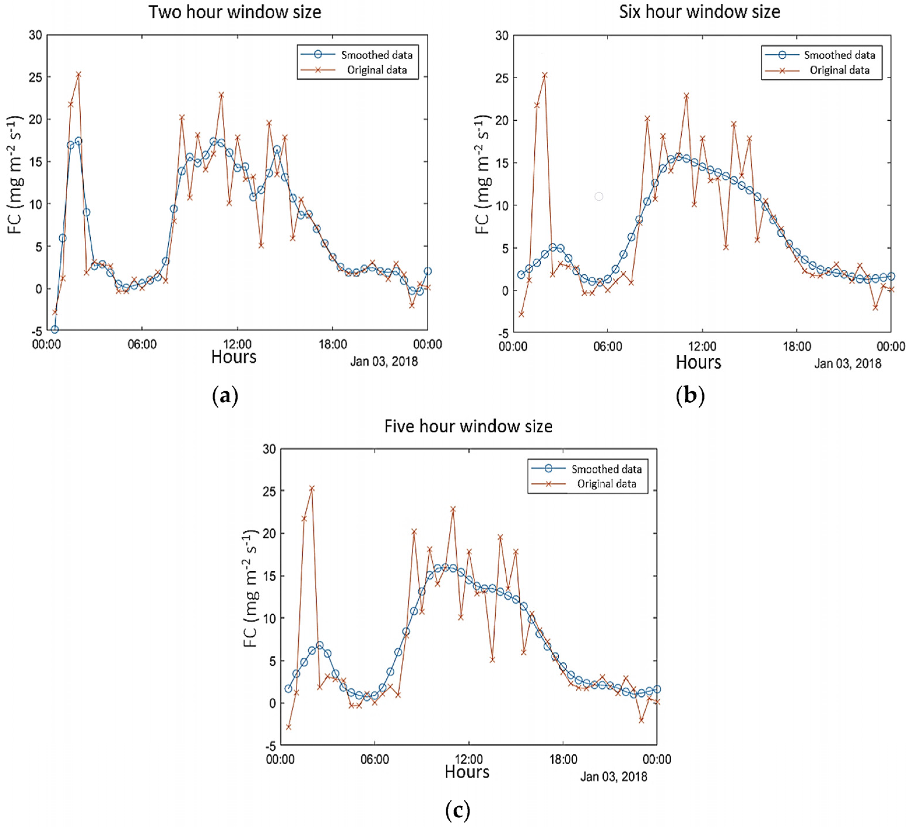
To remove outliers, the “filloutliers” function was used, which replaces the value that exceeds three times the standard deviation of the mean by the next value in the database. The “smoothdata” function was also used, which allows the elimination of “NaN” values and smooths the behavior of the data (Figure 6), through the application of a moving average according to a data window assigned by the user. An appropriate window for the smoothing method should be chosen carefully; if the window is too narrow, the smoothing carried out is insignificant, while if it is too wide, important dynamic behavior is likely to be lost. Figure 6a,b illustrate these two possibilities. In this work, it is found that a data window of five hours (Figure 6c) is appropriate to maintain desired dynamic information while removing the presence of noise and outliers.

2.5. Estimation of Energy Flows

For the training of both models, it will be necessary to generate energy flows, which will be determined using the EC method, considering the vertical speed of the wind, CO_2, and H₂O concentrations, among other variables recorded by the tower. Equation (9) was used to determine H, (10) for LE, and (11) for FC.

$$\mathrm{H}={\mathsf{\rho }}_{\mathrm{a}}{\mathrm{C}}_{\mathrm{p}}\overline{{\mathrm{w}}^{\prime }{\mathrm{T}}^{\prime }}$$

(9)

$$\mathrm{LE}={\mathrm{L}\mathsf{\rho }}_{\mathrm{a}}\overline{{\mathrm{w}}^{\prime }{\mathrm{e}}^{\prime }}$$

(10)

$$\mathrm{FC}=\overline{{{{\mathrm{w}}^{\prime }\mathsf{\rho }}_{\mathrm{c}}}^{\prime }}$$

(11)

where, ${\mathsf{\rho }}_{\mathrm{a}}$ is the air density, ${\mathrm{C}}_{\mathrm{p}}$ is the specific heat, ${\mathrm{w}}^{\prime }$ the deviation in the vertical speed of the wind, ${\mathrm{T}}^{\prime }$ is the deviation in the instantaneous temperature, ${{\mathsf{\rho }}_{\mathrm{c}}}^{\prime }$ is the deviation in the density of the CO₂ present in the air, ${\mathrm{e}}^{\prime }$ is the deviation in vapor pressure and $\mathrm{L}$ is the latent heat of vaporization.

A Pearson coefficient-based correlation analysis is carried out between the recorded meteorological variables, as well as the energy flows calculated using the EC method, allowing us to know the influence that some variables may have regarding the behavior of the energy flows.

Considering the variability of the recorded data, a time interval was selected where each variable maintained a controlled behavior, using measurements every 10 minutes from 01/01/2018 00:10 to 12/01/2018 23:50, generating a total of 1727 measurements. The RStudio Software (version 1.3.1093, Boston, MA, USA. Available online: https://www.rstudio.com/, accessed on 10 June 2021) is used for data processing, through the “cor()” and “corplot()” functions which allow obtaining the correlation plot with their respective values.

2.6. Neural Network Configuration

A deep feedforward neural network was used to model the desired outputs. To structure the neural network, the “Experiment Manager” application was used, which creates machine learning-based experiments through different conditions and hyperparameters. Once configured, the Experiment Manager scans the ranges assigned to each hyperparameter, determining the optimal values according to the performance criteria, in this case, it is the Root Mean Squared Error (RMSE) (12) of the test set output:

$$\mathrm{RMSE}=\sqrt{\frac{1}{\mathrm{n}}{\displaystyle \sum }_{\mathrm{d}=1}^{\mathrm{n}}{({\mathrm{x}}_{\mathrm{d}}-{\widehat{\mathrm{x}}}_{\mathrm{d}})}^2}$$

(12)

where ${\mathrm{x}}_{\mathrm{d}}$ represents the estimated value and ${\widehat{\mathrm{x}}}_{\mathrm{d}}$ is the actual value for n number of observations. The hyperparameters considered to carry out the experiments are as follows:

• Training_days: Due to the variability that may exist in data that depend on weather conditions, a training range was established that goes between 1 to 15 days, where the algorithm determines the number of days necessary for the best performance of the model.
• Hidden_layers: According to [55] using one to two hidden layers could be enough to obtain a meaningful model, while for [47] the structure of the network depends directly on the data. The number of hidden layers for this work varied between 2 and 9.
• HiddenUnits: Represents the number of neurons within each hidden layer. Varies from 10 to 100.
• MiniBatchSize: Refers to the number of samples considered before updating the weights and bias of the neural network. The lot size is varied between 16 and 128.
• InitialLearnRate: Controls the adjustment of the model parameters concerning the value of the loss function. The higher the learning rate, the more abrupt the adjustments in the parameters will be, which can cause the model to not reach the global minimum. The optimal learning rate is determined by varying it between 1 × 10⁻⁴ to 1 × 10⁻² [56].
• Inputs considered: Five fixed inputs were used, wind speed in its three components, CO_2, and H₂O absorptance. Additionally, the model could select the following variables recorded at the top of the tower: average wind speed (WS_ms_top_Avg), average wind direction (WindDir_D1_WVT), air temperature (temp10_Avg), and relative humidity (RH10_Avg), so that the algorithm can use the settings that benefit the estimate.
• Variables estimated by the model (outputs): The model will be estimating variables such as ${\mathsf{\Psi }}_{\mathrm{air}}$, FC, H, and LE.

3. Results

3.1. Relevant Variables in the Energy Flow Behavior

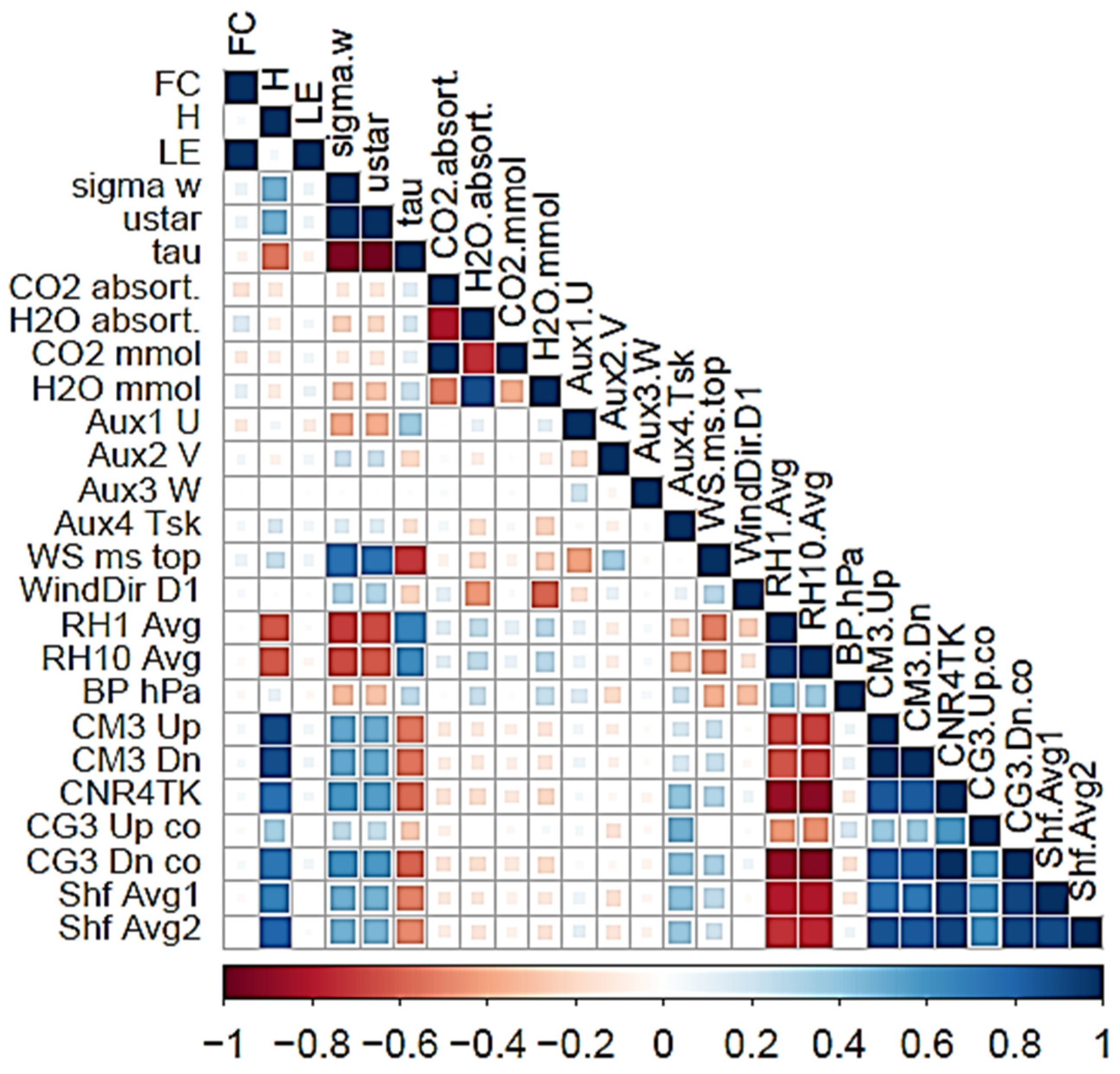
The Pearson correlation analysis performed using the variables recorded in the field of study served to identify which of these have a significant influence on the behavior of the energy flows analyzed. The variables considered for the analysis were: FC, H, LE, WS_ms_top_Avg, WindDir_D1_WVT, RH10_Avg and RH1_Avg, sonic temperature (Aux 4—Ts), wind speeds in its different components (U, V, and W), CO₂, and H₂O absorptance, the record of CO₂ and H₂O in mmol, barometric pressure (BP_hPa), average air temperature (CMR4TK), incoming and reflected shortwave radiation (CM3_Up and CM3_Dn), descending and ascending longwave radiation (CG3_Up_co and CG3_Dn_co), ground heat fluxes (Shf_Avg1 and Shf_Avg2), vertical velocity standard deviation (Sigma_w), friction velocity (ustar), and momentum (Tau).

The result of the analysis using Rstudio Software is shown in Figure 7, while the variables that presented significance (p < 0.001, R > 0.7) are shown in

Table 2. Significant correlations obtained (R > 0.7).

	H	Shf_avg1	Shf_avg2	Sigma_w	Ustar
CM3_up	0.90	0.73	0.86
CM3_dn	0.89	0.71	0.84
CNR4TK	0.74	0.89	0.92
Shf_avg2	0.80
CG3_dn	0.73	0.91	0.91
Ws_ms_top_Avg				0.75	0.74

.

3.2. Energy Flows Estimation through the Black Box Model

The proposed black box model was applied to January and September 2018, using the first 15 days of each month for model training, and then performing the testing process with any remaining day of the month. The values initially assigned to the hyperparameters are shown in

Table 3. Initial configuration of hyperparameters for the black box model.

Hyperparameters	Range
Initial Learn Rate	[1 × 10−4, 1 × 10−2]
Mini Batch Size	[16, 128]
Training days	[1, 15]
Hidden layers	[1, 8]
Hidden Units	[10, 100]

, while the optimal values according to the model for January and September 2018 are presented in

Table 4. Hyperparameters of the model for January 2018.

Hyperparameters	LE	FC	H	${\mathsf{\Psi }}_{\mathbf{air}}$
Initial Learn Rate	0.0094	0.0033	0.0048	0.0100
Mini Batch Size	106	110	71	47
Training days	15	8	12	14
Hidden layers	3	3	9	7
Hidden Units	84	61	94	13
RMSE test	3715.37	1.62	0.42	0.96
Additional variables	a, b, c	a, b, d	a, b	c, d

LE (W/m²), FC (mg/m²s), H (W/m²) and ${\mathsf{\Psi }}_{\mathrm{air}}$ (MPa). Here “a” represents WS_ms_top_Avg, “b” is WinDir_D1_WVT, “c” is temp10_Avg, and “d” is RH10_Avg.

and

Table 5. Hyperparameters of the model for September 2018.

Hyperparameters	LE	FC	H	${\mathsf{\Psi }}_{\mathbf{air}}$
Initial Learn Rate	0.0008	0.0098	0.0098	0.0010
Mini Batch Size	27	31	20	38
Training days	4	10	6	15
Hidden layers	8	8	6	9
Hidden Units	10	99	10	40
RMSE test	2968.40	1.95	0.44	0.56
Additional variables	a, b, c, d	d	-	a, b, c, d

LE (W/m²), FC (mg/m²s), H (W/m²) and ${\mathsf{\Psi }}_{\mathrm{air}}$ (MPa). Here “a” represents WS_ms_top_Avg, “b” is WinDir_D1_WVT, “c” is temp10_Avg, and “d” is RH10_Avg.

, respectively, being used for validation on 25 January and 25 September.

From Table 4 and Table 5 can be observed the difference in the hyperparameters depending on the training dataset used. These differences can be attributed to the season in which the training data are collected. At the location, January corresponds to one of the driest months, while September belongs to the rainy season. These different weather conditions, as well as the possible discrepancies in data recollection, could explain the variation in hyperparameters’ optimal values.

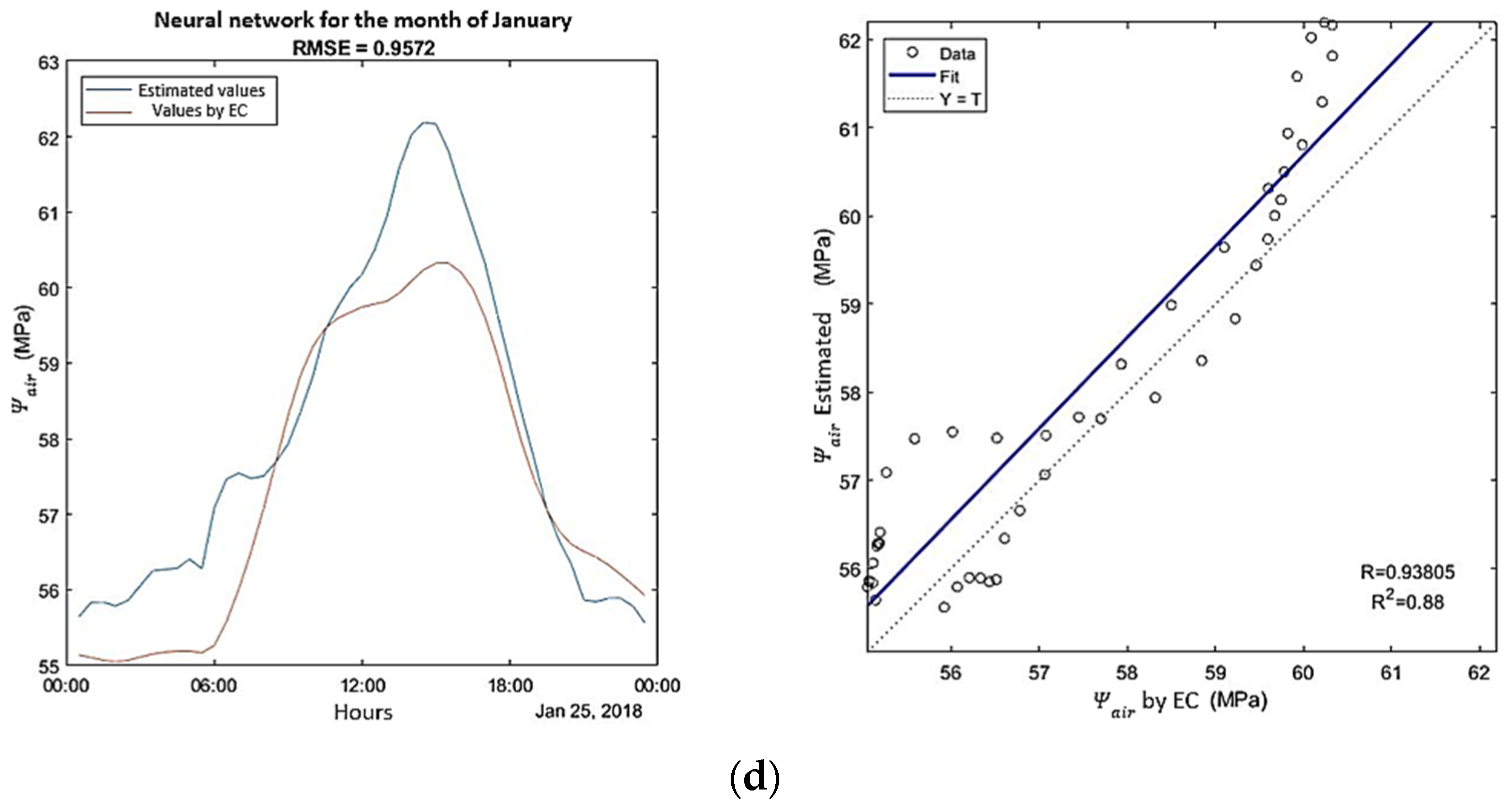
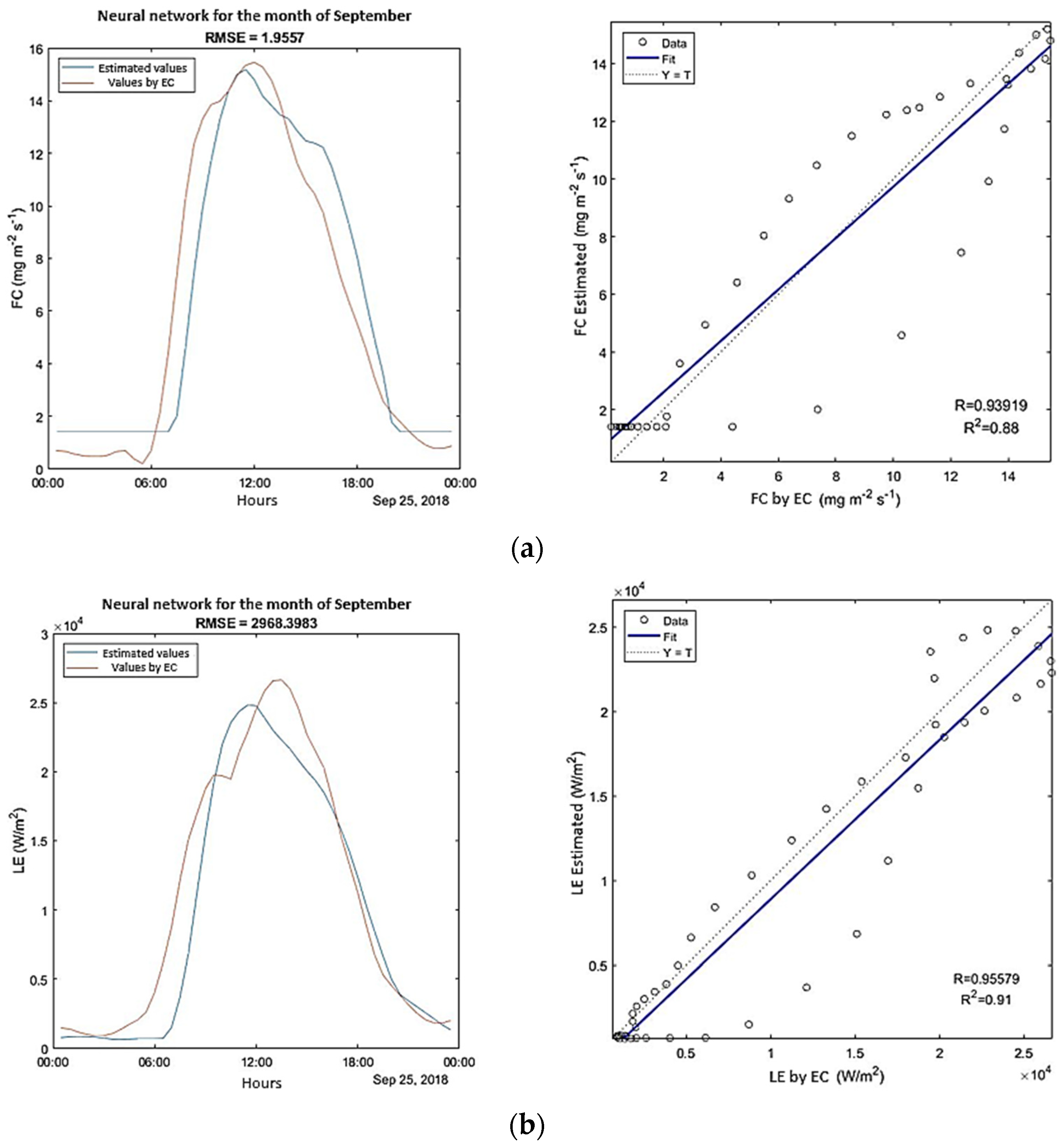
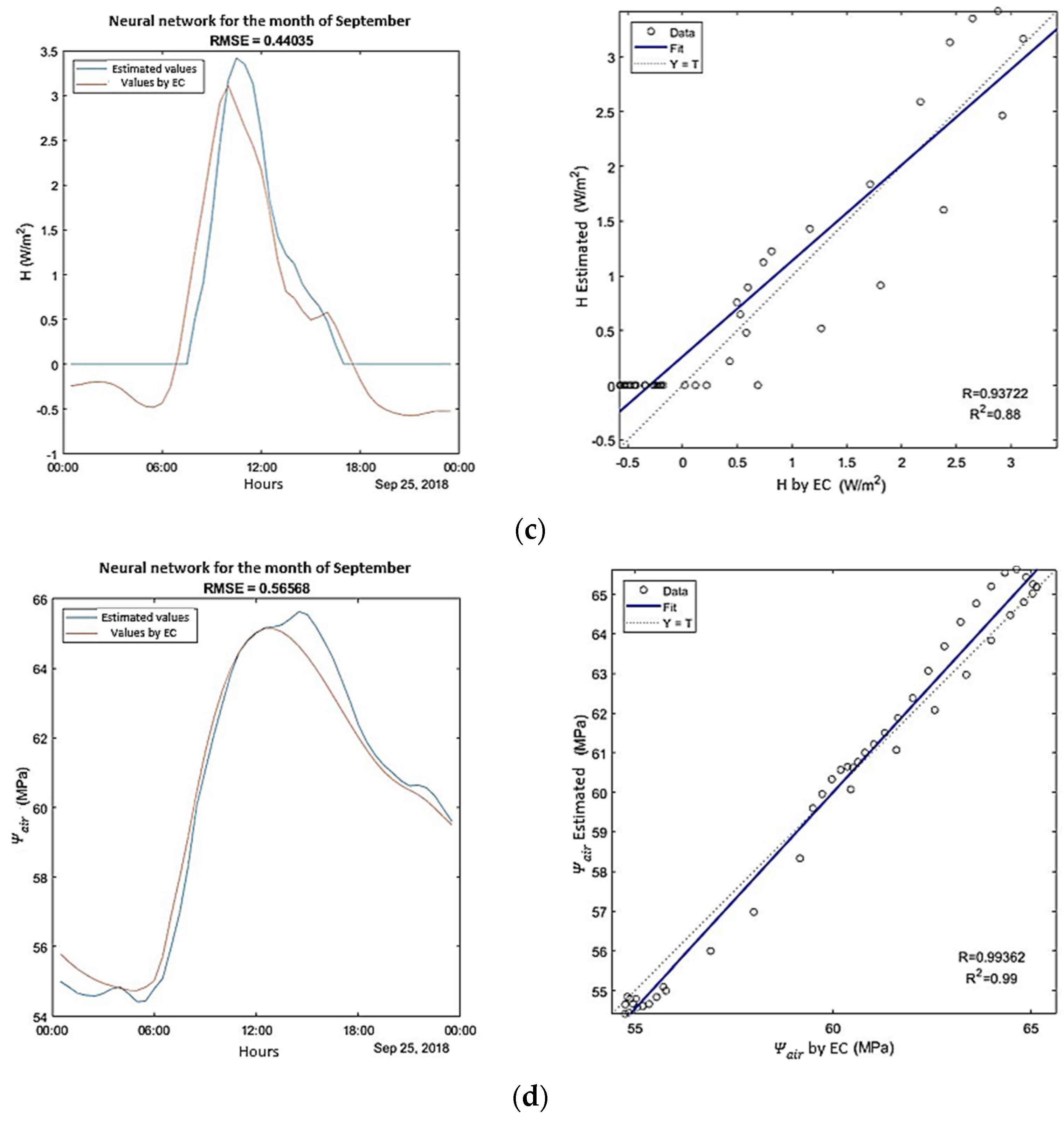
Obtaining the most efficient configuration for the hyperparameters, we proceed to estimate the energy fluxes for FC, LE, H, and ${\mathsf{\Psi }}_{\mathrm{air}}$ presented in sections a, b, c, and d for January (Figure 8) and September (Figure 9). For January, FC obtained an R² value of 0.95 (Figure 8a), while for September it decreased to 0.88 (Figure 9a). For LE there was also a reduction in the R² coefficient from 0.93 to 0.91 (Figure 8b and Figure 9b), however, for H and ${\mathsf{\Psi }}_{\mathrm{air}}$ there was an increase when comparing the months, from 0.86 (Figure 8c) to 0.88 (Figure 9c) and from 0.88 (Figure 8d) to 0.99 (Figure 9d), respectively.

3.3. Water Potential in Air through the Grey Box Model

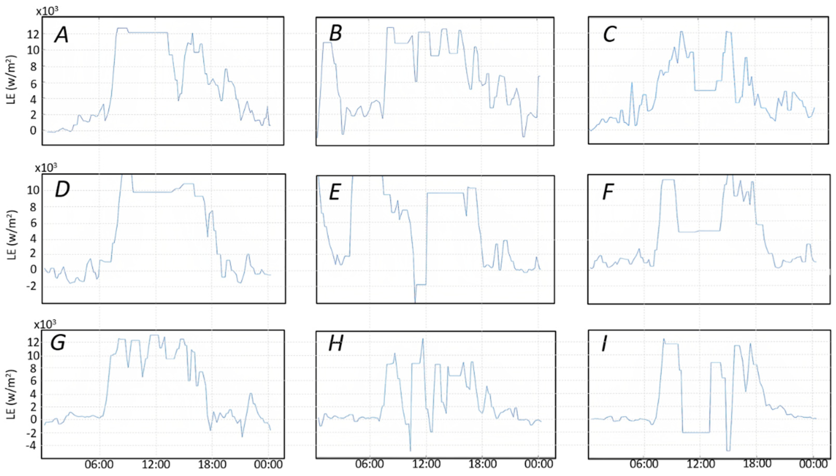
The data that were used in the grey box model were based on the daily behavior presented by the input variable LE, from 1 January 2018 to 26 June 2018, whose common behaviors are shown in Figure 10. Test runs were made using each of the nine behaviors, where group G managed to generate the lowest estimated error value.

The gray box model presented disadvantages regarding the ability to predict the variable of interest using highly variable data for the training period, which is why it was proposed to use days that had a similar behavior for the LE variable, resulting in an increase of the R². In the case of the black box model, neural networks and their different layers allow much more complex data to be analyzed, so it was not necessary to group similar days to be used during training. Considering that our range of data is not the same for each model presented, it would not be appropriate to try to compare them between them even though the R² can be obtained in both models.

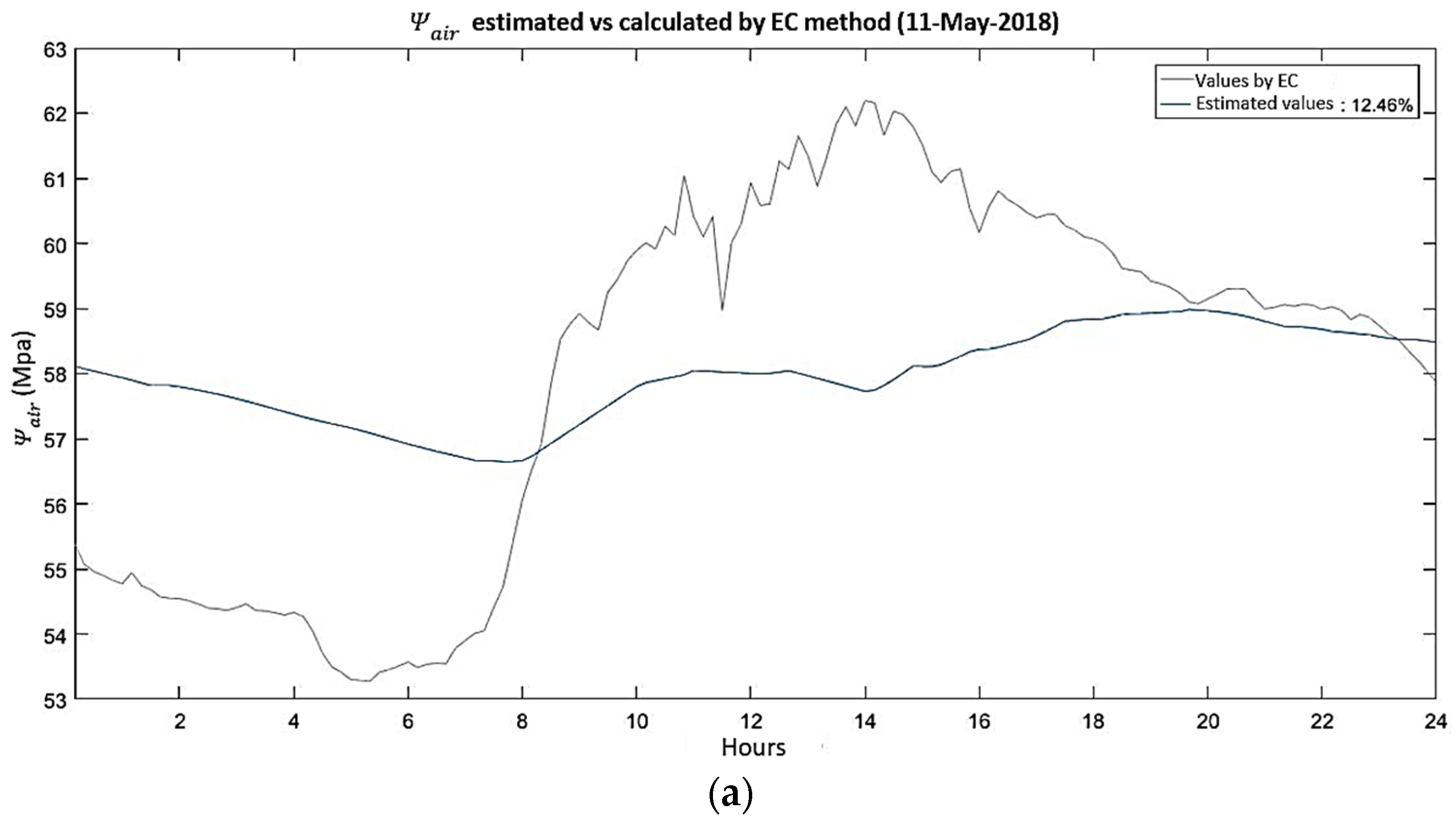
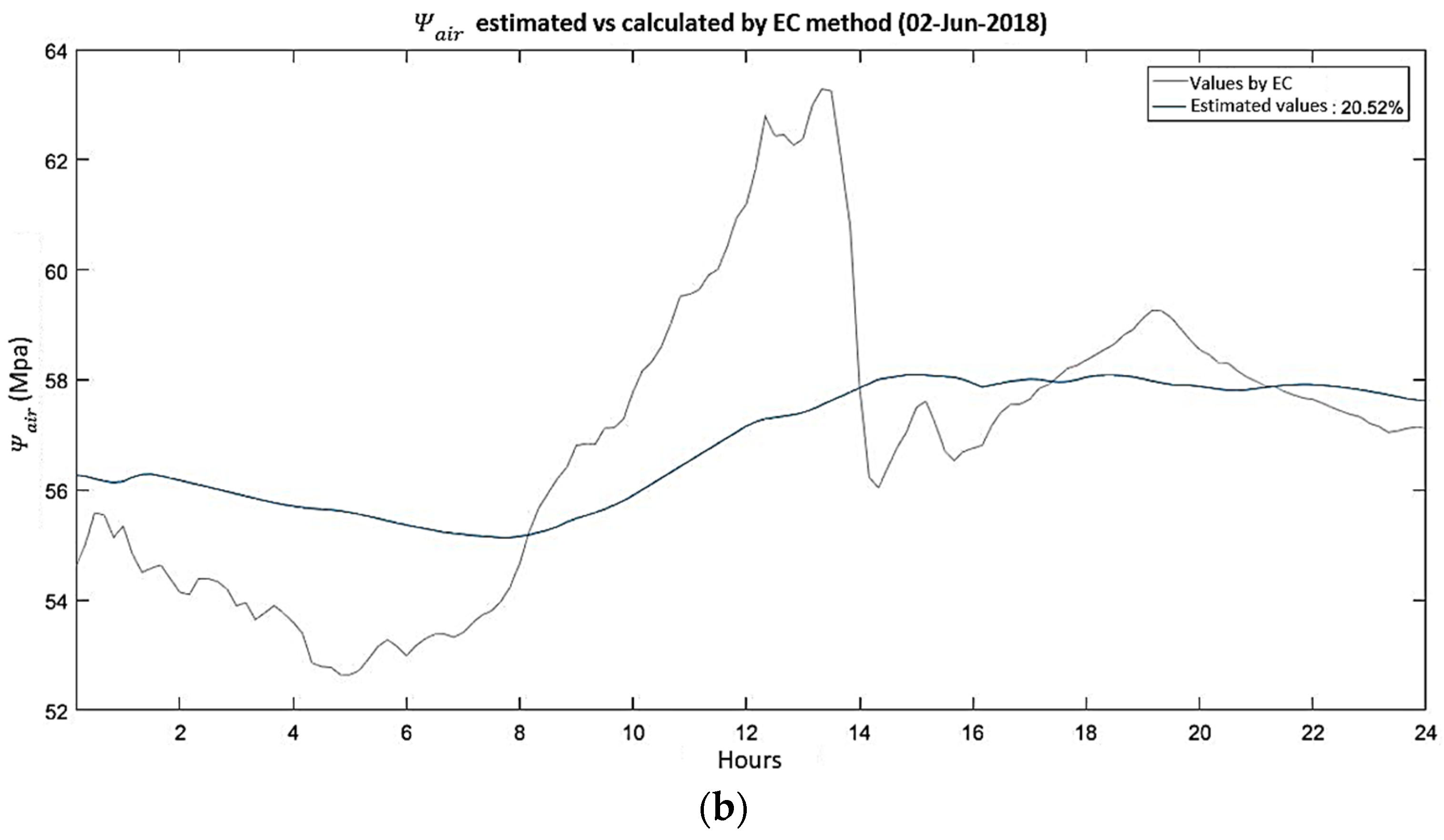
Once the model determines the configuration of R, C, and G that minimizes the estimation error value (

Table 6. Results of the iterations for the grey box model.

Parameters	Initial Values	Estimated by the Model
C	2.2501 × 104	8.8027 × 104
R	6.1451 × 105	4.8222 × 104
G	0.1112	4.2418 × 109

), the data are used for the validation process, estimating the ${\mathsf{\Psi }}_{\mathrm{air}}$ value for 11 May and 2 June (days that did not belong to the training group), comparing it with ${\mathsf{\Psi }}_{\mathrm{air}}$ obtained by the EC method. The training process of this model generated an estimation error value of 13.46% after 4774 iterations. The results obtained in the validation of 11 May (Figure 11a) show an R² coefficient of 0.37, while for 2 June (Figure 11b) an R² coefficient of 0.43 was obtained, both representing a very low ability to predict the behavior of ${\mathsf{\Psi }}_{\mathrm{air}}$.

4. Discussion

The correlation analysis carried out showed a weak relationship between the variables recorded and the resulting energy flows, where only the sensible heat flux obtained a significant relationship with the values of shortwave radiation, heat flux in the ground, sonic temperature, and the long wave ascending radiation. The analysis showed negative correlation values in long wave ascending radiation, sonic temperature, and heat flux in the ground when related to the relative humidity of the medium (−0.92, −0.90, and −0.81, respectively). Negative correlations tend to be a common behavior within the analysis of flows in ecosystems according to [57], where the correlation that existed between the temperature at different points of the forest (soil, air) and the net exchange of the ecosystem was analyzed.

Similarly, the authors in [58] carried out a correlation analysis between the CO₂ content in the soil and some measured variables such as pressure, air temperature, soil temperature, and friction speed. No significant correlation was observed between barometric pressure and the other variables recorded, but a correlation between friction speed and wind speed was observed (R = 0.74, p < 0.001), comparable to the work performed in [59], in addition to a correlation between sensible heat flux and net radiation.

Regarding the energy flow estimation, the study presented in [60] made an approximation of the value of H in an arid zone, using the atmospheric similarity theory for the second moment of air temperature. The model results were compared with the calculations generated by the EC method, whose R² coefficient was 0.85. The study [21] presented a record of LE comparisons at different points using a Bayesian model involving five algorithms: Moderate Resolution Imaging Spectroradiometer (MODIS), Penman–Monteith for remote sensing, Priestley Taylor based on LE, Modified Satellite-based Priestley Taylor (MS-PT), and Penman’s semi-empirical algorithm for LE, obtaining R² values greater than 0.7. In [22], the Shuttleworth and Wallace (SW) model was used to determine the value of LE on a vineyard in the Maule region, Chile. This model consisted of combining two one-dimensional models regarding crop transpiration and soil evaporation. The results of the SW model were compared with the EC method, obtaining an R² coefficient of 0.77.

Some works where neural networks are used to determine energy flows are [28] estimating FC (0.45 < R² < 0.72) and LE (0.51 < R² < 0.85) for six coniferous forests in Europe, while in [29] the R² coefficient for FC was between 0.59 and 0.79, while for LE it was between 0.83 and 0.88 in a coniferous forest in the United States. The work of [19] developed on a corn plantation was also analyzed, obtaining values for LE greater than 0.95 and for H greater than 0.80 concerning the coefficient of determination R².

The aforementioned models are analyzed, using the R² coefficient to compare the effectiveness of some models used according to the literature, where it can be seen that neural networks as an estimation/prediction method turn out to be very effective. In this study, the estimates of LE (R² > 0.91), H (R² > 0.86), FC (R² > 0.88) and ${\mathsf{\Psi }}_{\mathrm{air}}$ (R² > 0.88) represent a prediction that is fairly close to the real data.

The grey box model developed using the state space representation solution shows a low fit to the data calculated using the EC method, 12.45% and 20.52% for May and June, respectively. In contrast, the use of the cohesion-tension theory in other works requires the use of multiple equations, but its usefulness lies in the fact that the authors have the information regarding each of the variables considered (hydraulic conductances, specific conductivity of branches and leaves, potentials, among others) [38,42,61,62]. Overall, considering the results obtained, the consideration of the non-linear behavior, involving many other variables may help increase the effectiveness of the model.

The use of the grey box model to determine the variables that explained some phenomena was used by [52] to represent the thermal dynamics that exist in buildings in humid and rainy climates. At least 10 different configurations were proposed for the RC Networks. The output of the model used in the investigation was the internal temperature of the enclosure, generating RMSE values of 0.3573 °C and 0.99 °C for each case presented, implying a good predictive capacity of the model. The use of RC networks for space conditioning systems has proven to be very efficient, adjusting satisfactorily to the real conditions of the phenomenon [63,64,65]. However, the application to the behavior of trees would require further study regarding the structuring and selection of the variables that would explain the phenomenon, based on the results obtained within this investigation.

By mentioning the characteristic species of the study area, it was intended to be able to determine the coefficients related to storage and resistance to the flow of water, using the gray box model, whose results would be compared with existing data in the literature (A. germinans). Because the results generated by the gray box model for R, C, and G did not correspond to physical behavior, it was not possible to obtain the hydrological characteristics of the trees using the LE record of the tower as the input value.

5. Conclusions

This work proposed the use of two methods for the estimation of parameters that describe the behavior of the mangrove forest of the Bay of Panama, carrying out a bibliographic review of the models used, as well as the development of a methodology for the processing of meteorological data that would be used in the investigation.

In the development of a correlation analysis between the registered variables, the significance could be observed only with H and the heat flux in the soil. Within the period analyzed, the sensor that measures photosynthetic active radiation (PAR) was not available, which would have had a direct correlation with FC according to the literature analyzed.

The adequate treatment of the data used was fundamental to obtain accurate results because the applied methods needed to find patterns among the data during the training process, to later predict the behavior during the validation of the model. The data recorded by the tower may have erroneous measurements due to the presence of some external phenomenon that affects its calibration. Likewise, the behavior of the wind and the climatic conditions can influence the presence of noise in the recorded data, so processing is recommended before using them in such a model.

Depending on the model, we have the following conclusions:

• Grey Box Model: The analogy of Ohm’s Law was applied to determine some characteristic parameters of the study area, such as hydraulic conductivity per tree (1/R) and water storage (C). The model used, as an input variable, the latent heat (LE) registered by the measurement tower, and by using the MATLAB software, the development of the equations in state space was obtained that would indicate the respective values for the resistances and capacitances existing in the model. Carrying out the respective runs for each month, it was not possible to obtain physical values that represented the behavior of the species, the system required more information to achieve the connection between the flows recorded by the tower and the conditions of the selected species. Nine behaviors were found and the one with the fewest variations was selected, and then validated with the days 11 May and 2 June. The model improved its ability to predict behavior, but the coefficient R² obtained was still low (0.37 and 0.43).
• Black Box Model: A black box model was applied and developed through the application of neural networks using the Deep Learning package of MATLAB software. The use of neural networks for the prediction of energy flows (LE, H, FC) was highly effective, obtaining R² values greater than 0.86 in the runs carried out in January and September 2018.

As mangrove areas are lost to the development of poorly planned economic activities, the efficiency with which mangrove forests manage to fix and store one of the gases that contribute to the greenhouse effect begins to reduce. The modification of the hydroperiod in these areas could accelerate the process of emission of gases such as methane, considering that the areas are exposed to the open sky [66]. From another perspective, maintaining and recovering these mangrove areas would represent direct support for the reduction of emissions in these areas, the main contribution of the research being the reinforcement of the process of obtaining data that allows showing the economic and environmental contribution of these areas for the generation and modification of government policies for the protection and rehabilitation of these ecosystems.

References

- Castro, M. Derretimiento de Los Polos: Evolución, Causas, Consecuencias, Soluciones—Lifeder. Available online: https://www.lifeder.com/derretimiento-de-los-polos/ (accessed on 17 August 2020).
- Food and Agriculture Organization of the United Nations. Carbono Orgánico Del Suelo: El Potencial Oculto; Food & Agriculture Org: Rome, Italy, 2017; ISBN 978-92-5-309681-7. [Google Scholar]
- Sjögersten, S.; de la Barreda-Bautista, B.; Brown, C.; Boyd, D.; Lopez-Rosas, H.; Hernández, E.; Monroy, R.; Rincón, M.; Vane, C.; Moss-Hayes, V.; et al. Coastal Wetland Ecosystems Deliver Large Carbon Stocks in Tropical Mexico. Geoderma 2021, 403, 115173. [Google Scholar] [CrossRef]
- Velázquez-Pérez, C.; Tovilla-Hernández, C.; Romero-Berny, E.I.; De Jesús-Navarrete, A. Mangrove Structure and Its Influence on the Carbon Storage in La Encrucijada Reserve, Chiapas, Mexico. Madera Y Bosques 2019, 25, 1–14. [Google Scholar] [CrossRef] [Green Version]
- Das, S.; Crépin, A.S. Mangroves Can Provide Protection against Wind Damage during Storms. Estuar. Coast. Shelf Sci. 2013, 134, 98–107. [Google Scholar] [CrossRef]
- Al-Khayat, J.A.; Abdulla, M.A.; Alatalo, J.M. Diversity of Benthic Macrofauna and Physical Parameters of Sediments in Natural Mangroves and in Afforested Mangroves Three Decades after Compensatory Planting. Aquat. Sci. 2018, 81, 4. [Google Scholar] [CrossRef]
- Richter, O.; Nguyen, H.A.; Nguyen, V.P. Modeling Phytoremediation by Mangroves. 2013. pp. 1–5. Available online: https://www.researchgate.net/publication/305446247_Modeling_Phytoremediation_by_Mangroves (accessed on 14 July 2021).
- Nguyen, A.; Le, B.V.Q.; Richter, O. The Role of Mangroves in the Retention of Heavy Metal (Chromium): A Simulation Study in the Thi Vai River Catchment, Vietnam. Int. J. Environ. Res. Public Health 2020, 17, 5823. [Google Scholar] [CrossRef] [PubMed]
- Shinde, P.S.; Donde, S.S. Heavy Metal Pollution Correlation with Mangrove (Avicennia Marina) Carbon Sequestration in Dahisar Creek of Mumbai Region, India. Ecol. Environ. Conserv. 2018, 24, S344–S348. [Google Scholar]
- Ray, R.; Dutta, B.; Mandal, S.K.; González, A.G.; Pokrovsky, O.S.; Jana, T.K. Bioaccumulation of Vanadium (V), Niobium (Nb) and Tantalum (Ta) in Diverse Mangroves of the Indian Sundarbans. Plant Soil 2020, 448, 553–564. [Google Scholar] [CrossRef]
- Pittarello, M.; Busato, J.G.; Carletti, P.; Sodré, F.F.; Dobbss, L.B. Dissolved Humic Substances Supplied as Potential Enhancers of Cu, Cd, and Pb Adsorption by Two Different Mangrove Sediments. J. Soils Sediments 2019, 19, 1554–1565. [Google Scholar] [CrossRef] [Green Version]
- FAO. The World’s Mangroves 1980–2005. A Thematic Study Prepared in the Framework of the Global Forest Resources Assessment 2005; FAO Forestry Paper; FAO: Roma, Italy, 2007; ISBN 978-92-5-105856-5. [Google Scholar]
- Hoyos, R.G.; Estela Urrego, L.G.; Lema, Á.T. Respuesta de La Regeneración Natural En Manglares Del Golfo de Urabá (Colombia) a La Variabilidad Ambiental y Climática Intra-Annual. Rev. De Biol. Trop. 2013, 61, 1445–1461. [Google Scholar] [CrossRef] [Green Version]
- Barr, J.G.; Engel, V.; Smith, T.J.; Fuentes, J.D. Hurricane Disturbance and Recovery of Energy Balance, CO2 Fluxes and Canopy Structure in a Mangrove Forest of the Florida Everglades. Agric. For. Meteorol. 2012, 153, 54–66. [Google Scholar] [CrossRef] [Green Version]
- Zhao, X.; Rivera-Monroy, V.H.; Farfán, L.M.; Briceño, H.; Castañeda-Moya, E.; Travieso, R.; Gaiser, E.E. Tropical Cyclones Cumulatively Control Regional Carbon Fluxes in Everglades Mangrove Wetlands (Florida, USA). Sci. Rep. 2021, 11, 13927. [Google Scholar] [CrossRef] [PubMed]
- Granados-Martínez, K.P.; Yépez, E.A.; Sánchez-Mejía, Z.M.; Gutiérrez-Jurado, H.A.; Méndez-Barroso, L.A. Environmental Controls on the Temporal Evolution of Energy and CO2 Fluxes on an Arid Mangrove of Northwestern Mexico. J. Geophys. Res. Biogeosciences 2021, 126, e2020JG005932. [Google Scholar] [CrossRef]
- Day, J.W.; Conner, W.H.; DeLaune, R.D.; Hopkinson, C.S.; Hunter, R.G.; Shaffer, G.P.; Kandalepas, D.; Keim, R.F.; Kemp, G.P.; Lane, R.R.; et al. A Review of 50 Years of Study of Hydrology, Wetland Dynamics, Aquatic Metabolism, Water Quality and Trophic Status, and Nutrient Biogeochemistry in the Barataria Basin, Mississippi Delta-System Functioning, Human Impacts and Restoration Approaches. Water 2021, 13, 642. [Google Scholar] [CrossRef]
- Vega-Cendejas, M.E.; Arreguín-Sánchez, F. Energy Fluxes in a Mangrove Ecosystem from a Coastal Lagoon in Yucatan Peninsula, Mexico. Ecol. Modell. 2001, 137, 119–133. [Google Scholar] [CrossRef]
- Safa, B.; Arkebauer, T.J.; Zhu, Q.; Suyker, A.; Irmak, S. Latent Heat and Sensible Heat Flux Simulation in Maize Using Artificial Neural Networks. Comput. Electron. Agric. 2018, 154, 155–164. [Google Scholar] [CrossRef]
- Burba, G.; Anderson, D. A Brief Practical Guide to Eddy Covariance CO2 Flux Measurements. Ecol. Appl. 2008, 18, 1368–1378. [Google Scholar]
- Yao, Y.; Liang, S.; Li, X.; Yang, H.; Fisher, J.B.; Zhang, N.; Chen, J.; Cheng, J.; Zhao, S.; Zhang, X.; et al. Bayesian Multimodel Estimation of Global Terrestrial Latent Heat Flux from Eddy Covariance, Meteorological, and Satellite Observations. J. Geophys. Res. 2014, 119, 6578–6595. [Google Scholar] [CrossRef]
- Ortega-Farias, S.; Carrasco, M.; Olioso, A.; Acevedo, C.; Poblete, C. Latent Heat Flux over Cabernet Sauvignon Vineyard Using the Shuttleworth and Wallace Model. Irrig. Sci. 2007, 25, 161–170. [Google Scholar] [CrossRef]
- Domingo, F.; Villagracia, L. ¿Cómo Se Puede Medir y Estimar La Evapotranspiración?: Estado Actual y Evolución. Ecosistemas 2003, 12, 1. [Google Scholar]
- Singh, R.K.; Irmak, A. Estimation of Crop Coefficients Using Satellite Remote Sensing. J. Irrig. Drain. Eng. 2009, 135, 597–608. [Google Scholar] [CrossRef]
- Er-Raki, S.; Rodriguez, J.C.; Garatuza-Payan, J.; Watts, C.J.; Chehbouni, A. Determination of Crop Evapotranspiration of Table Grapes in a Semi-Arid Region of Northwest Mexico Using Multi-Spectral Vegetation Index. Agric. Water Manag. 2013, 122, 12–19. [Google Scholar] [CrossRef]
- Huntingford, C.; Cox, P.M. Use of Statistical and Neural Network Techniques to Detect How Stomatal Conductance Responds to Changes in the Local Environment. Ecol. Modell. 1997, 97, 217–246. [Google Scholar] [CrossRef]
- Abareshi, B.; Schuepp, P.H. Sensible Heat Flux Estimation over the FIFE Site by Neural Networks. J. Atmos. Sci. 1998, 55, 1185–1197. [Google Scholar] [CrossRef]
- Van Wijk, M.T.; Bouten, W. Water and Carbon Fluxes above European Coniferous Forests Modelled with Artificial Neural Networks. Ecol. Modell. 1999, 120, 181–197. [Google Scholar] [CrossRef]
- Van Wijk, M.T.; Bouten, W.; Verstraten, J.M. Comparison of Different Modelling Strategies for Simulating Gas Exchange of a Douglas-Fir Forest. Ecol. Modell. 2002, 158, 63–81. [Google Scholar] [CrossRef]
- Qin, Z.; Su, G.; Zhang, J.; Ouyang, Y.; Yu, Q.; Li, J. Identification of Important Factors for Water Vapor Flux and CO2 Exchange in a Cropland. Ecol. Modell. 2010, 221, 575–581. [Google Scholar] [CrossRef]
- Qin, Z.; Su, G.L.; Yu, Q.; Hu, B.M.; Li, J. Modeling Water and Carbon Fluxes above Summer Maize Field in North China Plain with Back-Propagation Neural Networks. J. Zhejiang Univ. Sci. 2005, 6, 418–426. [Google Scholar] [CrossRef] [Green Version]
- Qin, Z.; Yu, Q.; Li, J.; Wu, Z.Y.; Hu, B.M. Application of Least Squares Vector Machines in Modelling Water Vapor and Carbon Dioxide Fluxes over a Cropland. J. Zhejiang Univ. Sci. 2005, 6, 491–495. [Google Scholar] [CrossRef] [Green Version]
- Castañeda-Miranda, A.; Castaño, V.M. Smart Frost Control in Greenhouses by Neural Networks Models. Comput. Electron. Agric. 2017, 137, 102–114. [Google Scholar] [CrossRef]
- Campbell, G.S. Soil Physics with BASIC : Transport Models for Soil-Plant Systems; Elsevier: Amsterdam, The Netherlands, 1985; ISBN 9780080869827. [Google Scholar]
- Zhuang, J.; Yu, G.R.; Nakayama, K. A Series RCL Circuit Theory for Analyzing Non-Steady-State Water Uptake of Maize Plants. Sci. Rep. 2014, 4, 6720. [Google Scholar] [CrossRef] [PubMed] [Green Version]
- Lhomme, J.P.; Rocheteau, A.; Ourcival, J.M.; Rambal, S. Non-Steady-State Modelling of Water Transfer in a Mediterranean Evergreen Canopy. Agric. For. Meteorol. 2001, 108, 67–83. [Google Scholar] [CrossRef]
- Ye, Z.P.; Yu, Q. A Coupled Model of Stomatal Conductance and Photosynthesis for Winter Wheat. Photosynthetica 2008, 46, 637–640. [Google Scholar] [CrossRef]
- Huntingford, C.; Smith, D.M.; Davies, W.J.; Falk, R.; Sitch, S.; Mercado, L.M. Combining the [ABA] and Net Photosynthesis-Based Model Equations of Stomatal Conductance. Ecol. Modell. 2015, 300, 81–88. [Google Scholar] [CrossRef]
- Zweifel, R.; Steppe, K.; Sterck, F.J. Stomatal Regulation by Microclimate and Tree Water Relations: Interpreting Ecophysiological Field Data with a Hydraulic Plant Model. J. Exp. Bot. 2007, 58, 2113–2131. [Google Scholar] [CrossRef]
- Bentrup, F.-W. Water Ascent in Trees and Lianas: The Cohesion-Tension Theory Revisited in the Wake of Otto Renner. Protoplasma 2017, 254, 627–633. [Google Scholar] [CrossRef] [Green Version]
- Tyree, M. The Cohesion-Tension Theory of Sap Ascent: Current Controversies. J. Exp. Bot. 1997, 48, 1753–1765. [Google Scholar] [CrossRef] [Green Version]
- Tyree, M.T.; Ewers, F.W. The Hydraulic Architecture of Trees and Other Woody Plants. New Phytol. 1991, 119, 345–360. [Google Scholar] [CrossRef]
- Kumagai, T. Modeling Water Transportation and Storage in Sapwood—Model Development and Validation. Agric. For. Meteorol. 2001, 109, 105–115. [Google Scholar] [CrossRef]
- Brooks, J.; Chen, M.A.; Mora, D.; Tejedor-Flores, N. A Critical Review on Mathematical Descriptions to Study Flux Processes and Environmental-Related Interactions of Mangroves. Sustainability 2021, 13, 6970. [Google Scholar] [CrossRef]
- El Naqa, I.; Murphy, M.J. What Is Machine Learning? In Machine Learning in Radiation Oncology: Theory and Applications; El Naqa, I., Li, R., Murphy, M.J., Eds.; Springer International Publishing: Cham, Switzerland, 2015; pp. 3–11. ISBN 978-3-319-18305-3. [Google Scholar]
- Columbia Engineering Artificial Intelligence (AI) vs. Machine Learning | Columbia AI. Available online: https://ai.engineering.columbia.edu/ai-vs-machine-learning/ (accessed on 26 May 2022).
- Goodfellow, I.; Bengio, Y.; Courville, A. Deep Learning; MIT Press: Cambridge, MA, USA, 2016; Volume 26, ISBN 9780262035613. [Google Scholar]
- Kubat, M. Neural Networks: A Comprehensive Foundation by Simon Haykin, Macmillan, 1994, ISBN 0-02-352781-7. Knowl. Eng. Rev. 1999, 13, 409–412. [Google Scholar] [CrossRef]
- Jara-Rojas, F.; Ortega-Farías, S.; Valdés-Gómez, H.; Poblete, C.; del Pozo, A. Model Validation for Estimating the Leaf Stomatal Conductance in Cv. Cabernet Sauvignon Grapevines. Chil. J. Agric. Res. 2009, 69, 88–96. [Google Scholar] [CrossRef]
- Jones, H.G. Plants and Microclimate: A Quantitative Approach to Environmental Plant Physiology; Cambridge University Press: Cambridge, UK, 2013; ISBN 9780511845727. [Google Scholar]
- Ishida, A.; Yamamura, Y.; Hori, Y. Roles of Leaf Water Potential and Soil-to-Leaf Hydraulic Conductance in Water Use by Understorey Woody Plants. Ecol. Res. 1992, 7, 213–223. [Google Scholar] [CrossRef]
- Rivera, A.K.; Sánchez, J.; Austin, M.C. Parameter Identification Approach to Represent Building Thermal Dynamics Reducing Tuning Time of Control System Gains: A Case Study in a Tropical Climate. Front. Built Environ. 2022, 8, 1–18. [Google Scholar] [CrossRef]
- Laucevicius, C.; Olmedo, P.; Jenifer, B. Estimación de Reservas de Carbono En Manglares de Juan Díaz Bajo Enfoque Ecosistémico, Panamá; Toth Research & Lab: Panama City, Panama, 2019. [Google Scholar]
- Google Maps Google Maps. Available online: https://www.google.com/maps/@9.0171535,-79.4487525,14.96z (accessed on 27 July 2022).
- Maren, A.J.; Harston, C.T.; Pap, R.M. Handbook of Neural Computing Applications; Academic Press: Cambridge, MA, USA, 1990; ISBN 9780125460903. [Google Scholar]
- Design and Run Experiments to Train and Compare Deep Learning Networks—MATLAB—MathWorks América Latina. Available online: https://la.mathworks.com/help/deeplearning/ref/experimentmanager-app.html (accessed on 14 March 2022).
- Lasslop, G.; Migliavacca, M.; Bohrer, G.; Reichstein, M.; Bahn, M.; Ibrom, A.; Jacobs, C.; Kolari, P.; Papale, D.; Vesala, T.; et al. On the Choice of the Driving Temperature for Eddy-Covariance Carbon Dioxide Flux Partitioning. Biogeosciences 2012, 9, 5243–5259. [Google Scholar] [CrossRef] [Green Version]
- Pérez Sánchez, E. Comportamiento de Los Flujos Gaseosos de CO2 En El Suelo de Un Ecosistema Kárstico. Factores Que Índice Introducción Resultados; Universidad de Granada: Granada, Spain, 2009. [Google Scholar]
- Anandakumar, K. Sensible Heat Flux over a Wheat Canopy: Optical Scintillometer Measurements and Surface Renewal Analysis Estimations. Agric. For. Meteorol. 1999, 96, 145–156. [Google Scholar] [CrossRef]
- Albertson, J.D.; Parlange, M.B.; Katul, G.G.; Chu, C.-R.; Stricker, H.; Tyler, S. Sensible Heat Flux From Arid Regions: A Simple Flux-Variance Method. Water Resour. Res. 1995, 31, 969–973. [Google Scholar] [CrossRef] [Green Version]
- Sobrado, M.A. Relationship of Water Transport to Anatomical Features in the Mangrove Laguncularia Racemosa Grown under Contrasting Salinities. New Phytol. 2007, 173, 584–591. [Google Scholar] [CrossRef]
- Sobrado, M.A. Hydraulic Properties of a Mangrove Avicennia Germinans as Affected by NaCl. Biol. Plant. 2001, 44, 435–438. [Google Scholar] [CrossRef]
- Wang, Z.; Chen, Y.; Li, Y. Development of RC Model for Thermal Dynamic Analysis of Buildings through Model Structure Simplification. Energy Build. 2019, 195, 51–67. [Google Scholar] [CrossRef]
- Cui, B.; Fan, C.; Munk, J.; Mao, N.; Xiao, F.; Dong, J.; Kuruganti, T. A Hybrid Building Thermal Modeling Approach for Predicting Temperatures in Typical, Detached, Two-Story Houses. Appl. Energy 2019, 236, 101–116. [Google Scholar] [CrossRef]
- Massa Gray, F.; Schmidt, M. A Hybrid Approach to Thermal Building Modelling Using a Combination of Gaussian Processes and Grey-Box Models. Energy Build. 2018, 165, 56–63. [Google Scholar] [CrossRef]
- Gómez Junca, D.A. Almacenes de Carbono y Emisiones de Metano En Manglares Con Diferente Composición de Especies En La Costa de Veracruz, México. 2018. Available online: https://repositorio.unbosque.edu.co/handle/20.500.12495/5487 (accessed on 21 December 2022).
Figure 1.
A nonlinear model of a neuron. Reproduced with permission from [48], Neural networks: a comprehensive foundation by Simon Haykin, published by Cambridge University Press, 1999.
Figure 2.
Representation of the Soil-Tree-Atmosphere Domain. Own elaboration.
Figure 3.
The location of the mangrove area was analyzed in the Bay of Panama [54].
Figure 4.
Photograph of the tower installed in the study area. Own elaboration.
Figure 5.
Behavior found in the database. Own elaboration.
Figure 6.
(a) Data smoothing using reference data every two hours (data window); (b) Data smoothing using reference data every six hours; (c) Data smoothing using reference data every five hours. Own elaboration.
Figure 7.
Correlation analysis of the registered variables. Own elaboration.
Figure 8.
Validation of the neural network for January, comparing the estimates with the values calculated using the EC method for (a) FC, (b) LE, (c) H, and (d) , each with their respective linear regression. Own elaboration.
Figure 9.
Validation of the neural network for September, comparing the estimates with the values calculated using the EC method for (a) FC, (b) LE, (c) H, and (d) , each with their respective linear regression. Own elaboration.
Figure 10.
Behaviors observed in LE data from 00:10 to 23:50. The variability recorded by the sensors can be observed, with surpluses shown in (E), (B) and (C), absence of data for (F), (H) and (I), as well as an expected behavior for (A), (D) and (G). Own elaboration.
Figure 11.
Validation of the grey box model for (a) May and (b) June, in terms of the water potential in the air. Own elaboration.