
Morphometric, Meteorological, and Hydrologic Characteristics Integration for Rainwater Harvesting Potential Assessment in Southeast Beni Suef (Egypt)

Abstract
:1. Introduction
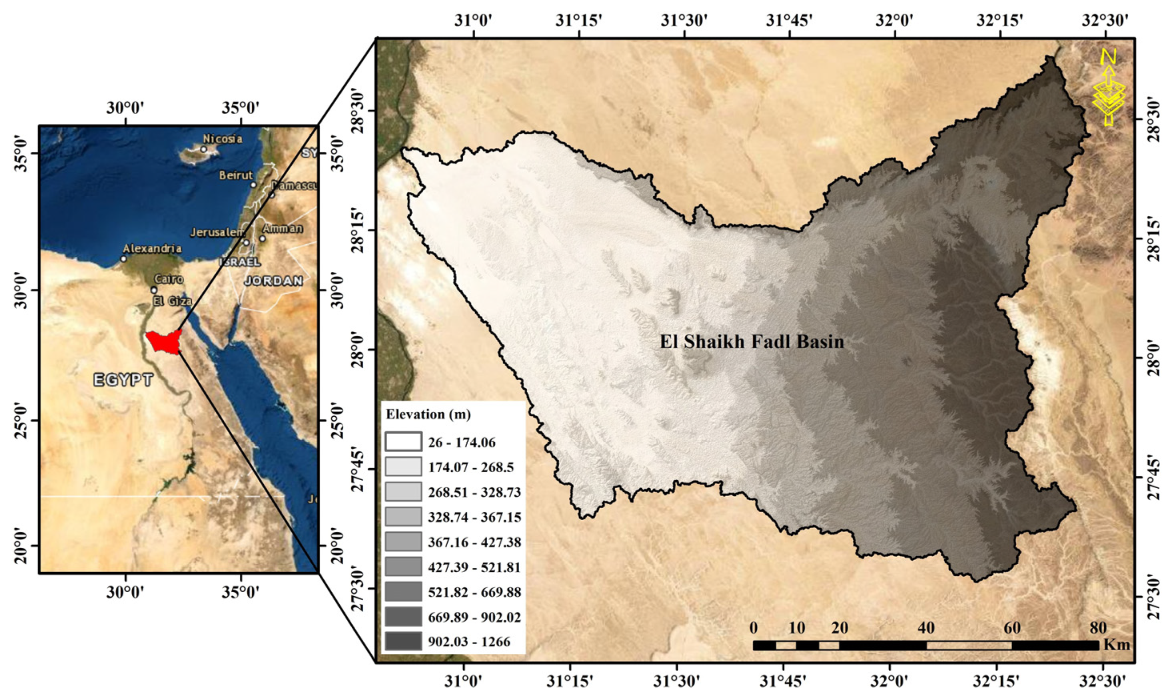
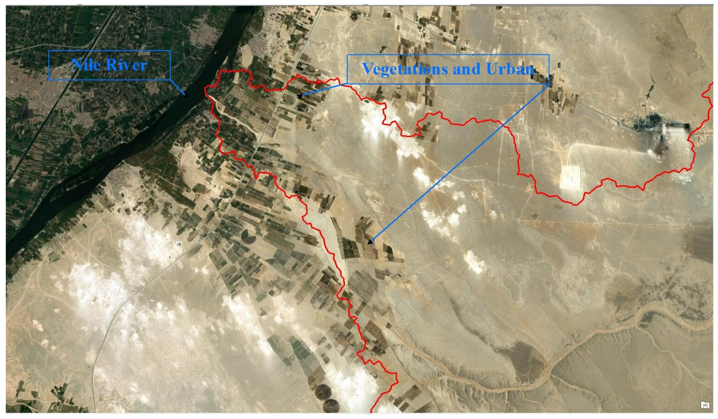
2. Study Area
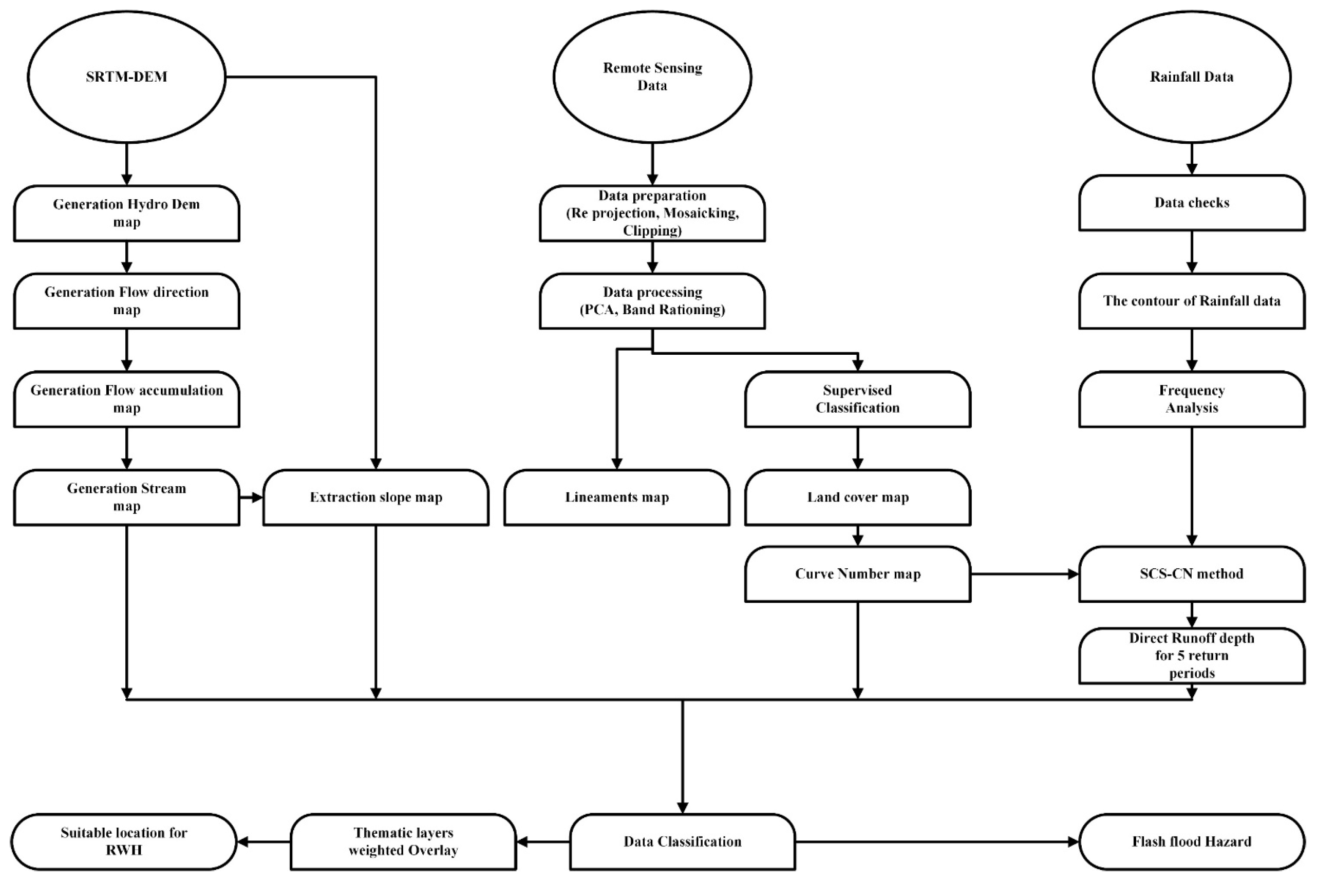
3. Materials and Methods
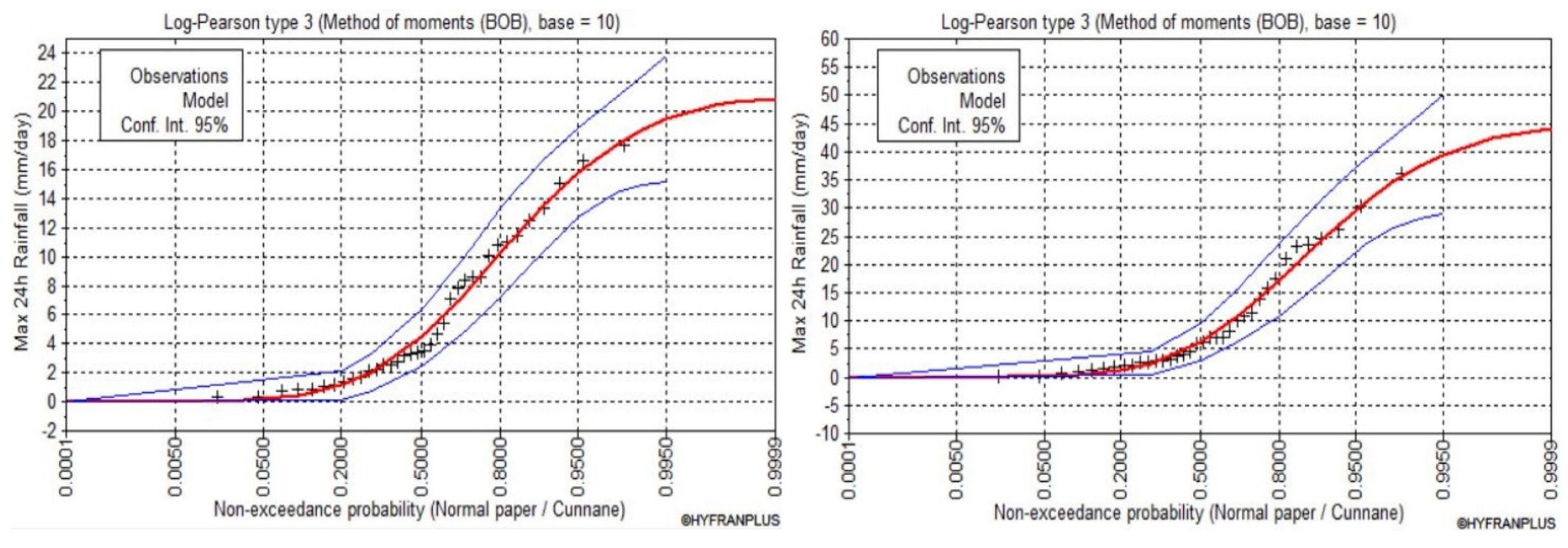
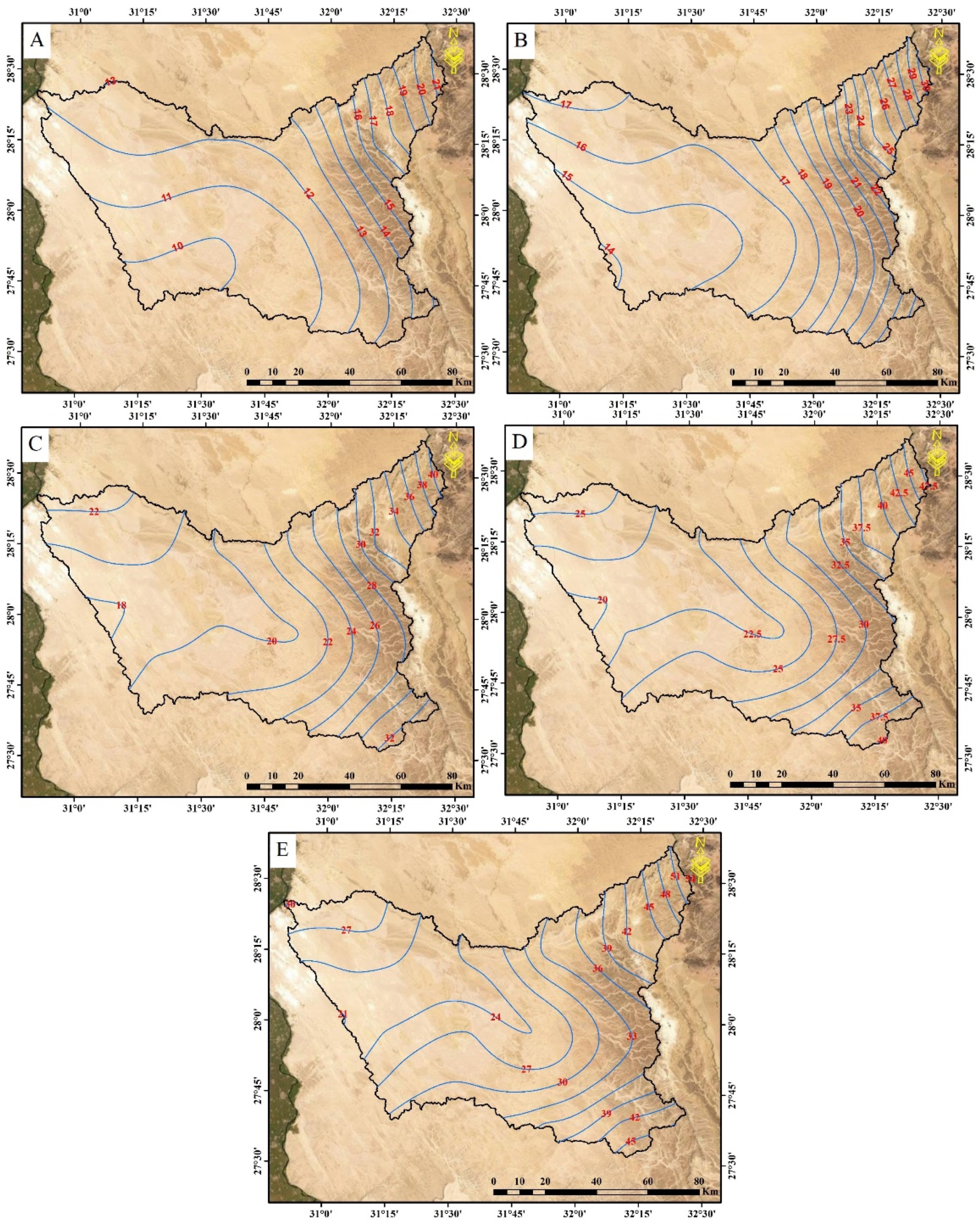
3.1. Rainfall Processing
3.2. Morphometric Analysis [45,46]
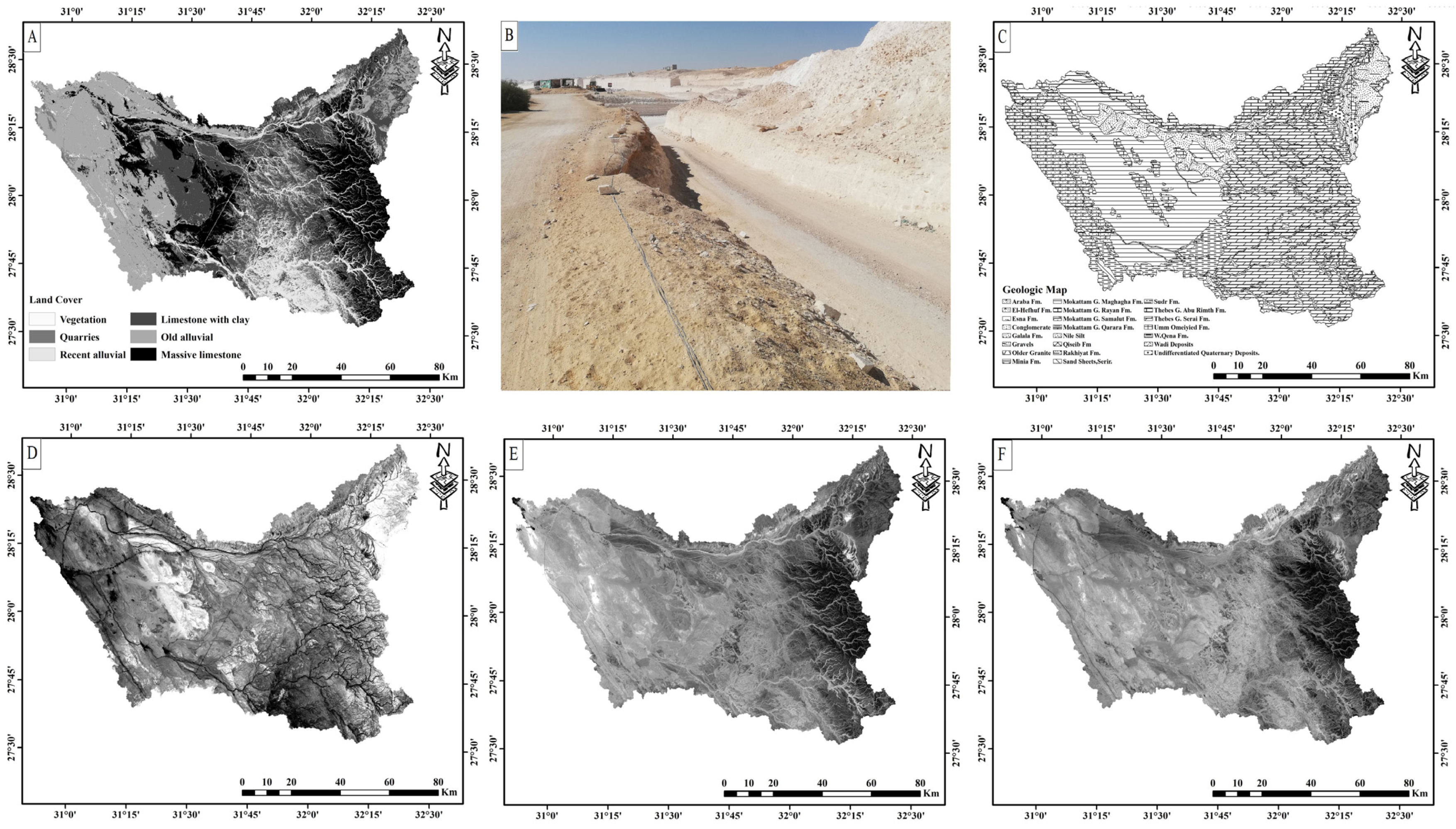
3.3. Image Analysis
3.4. Rainfall–Runoff Modeling
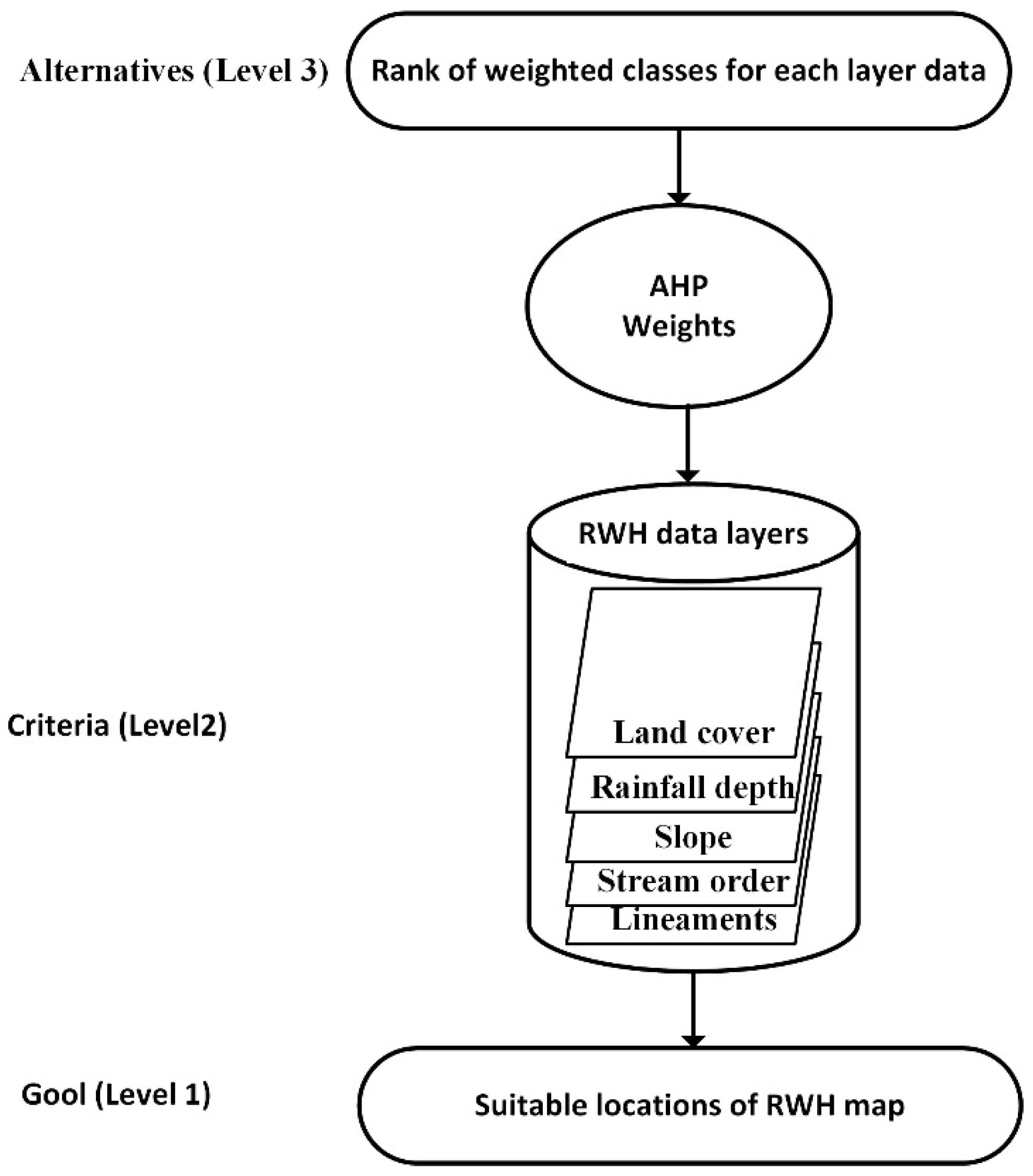
3.5. Mapping of the Suitable Potential Sites for RWH
4. Results and Discussion
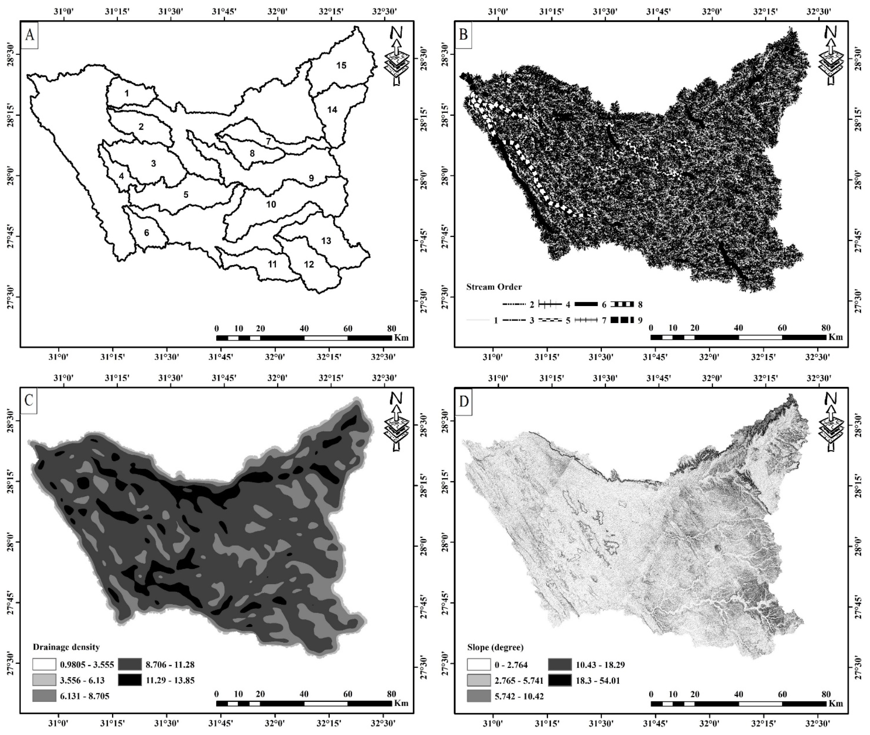
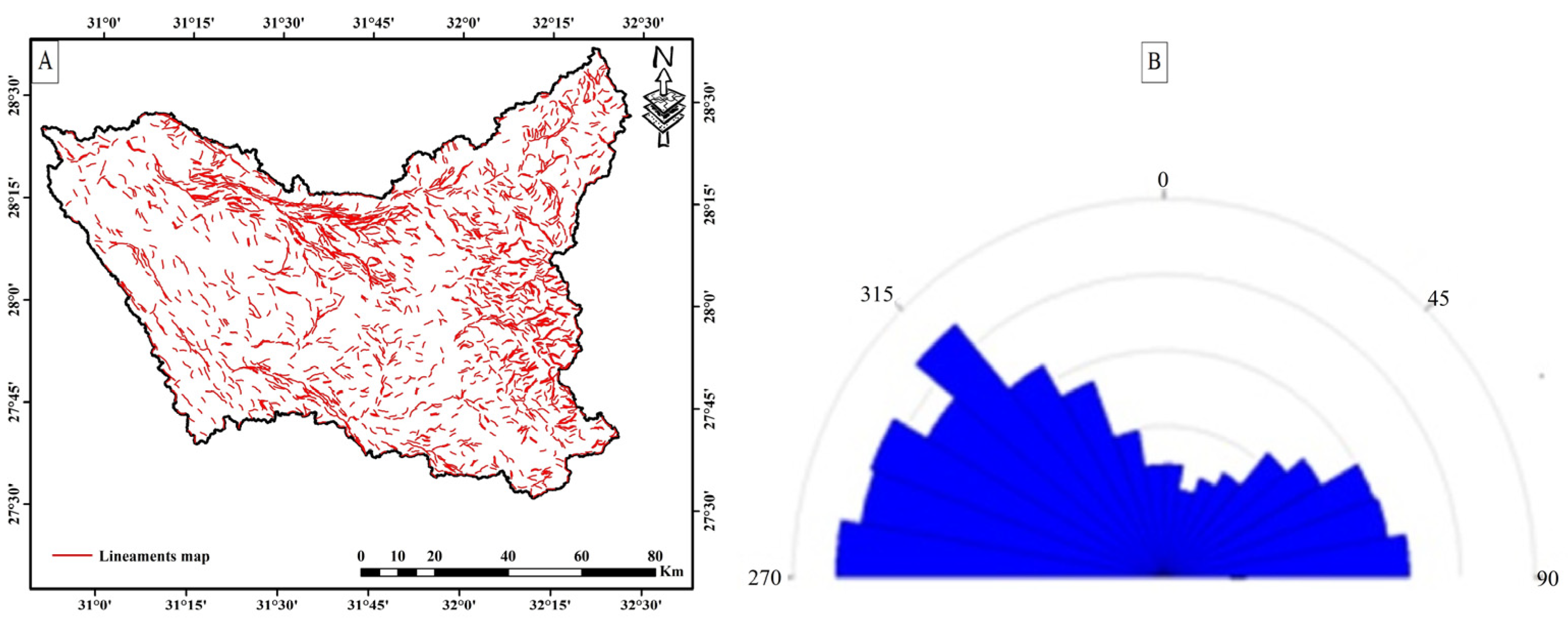
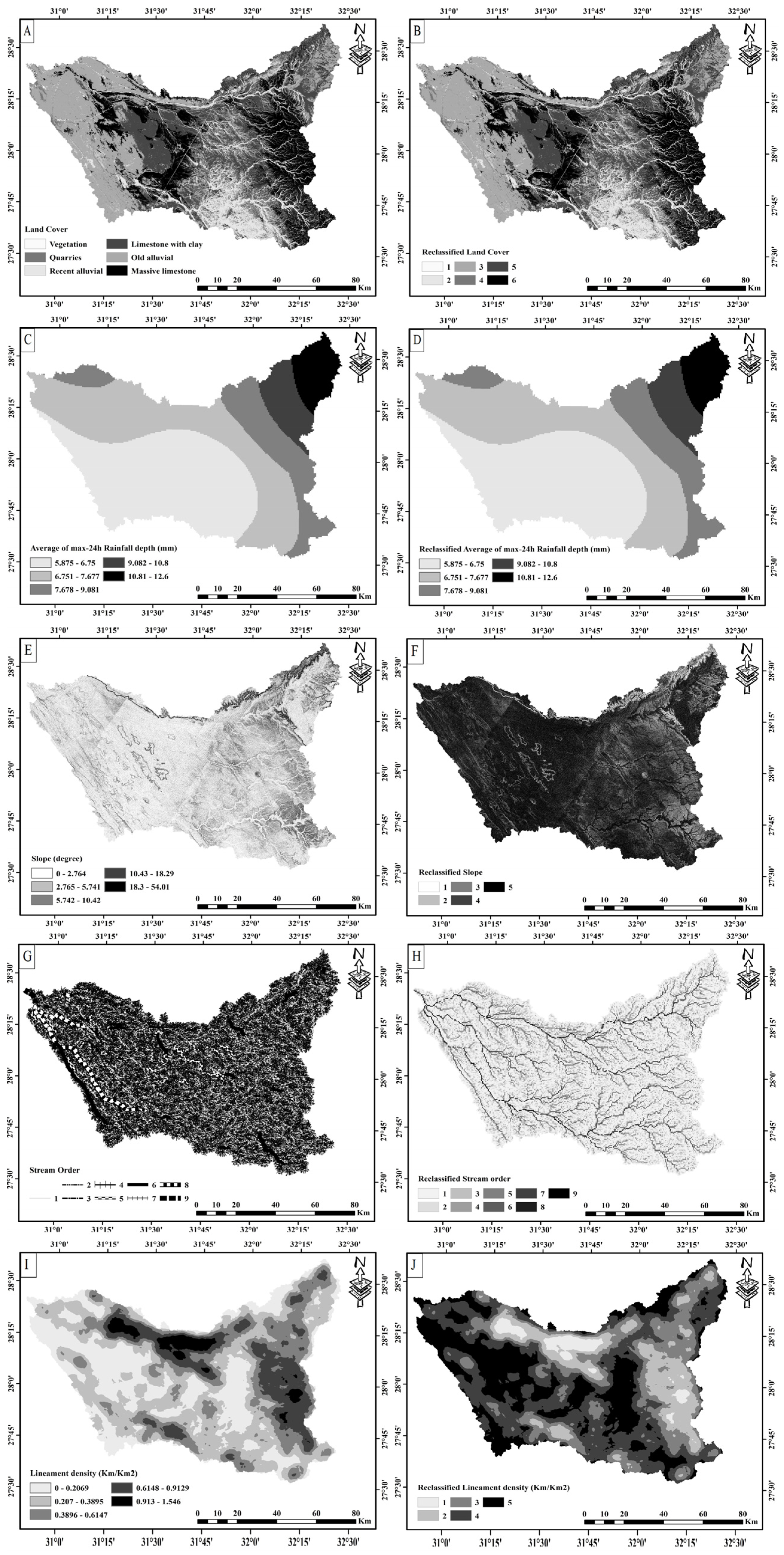
4.1. Morphometric Analysis
4.1.1. Linear Characteristics
4.1.2. Areal Characteristics
4.1.3. Relief Characteristics
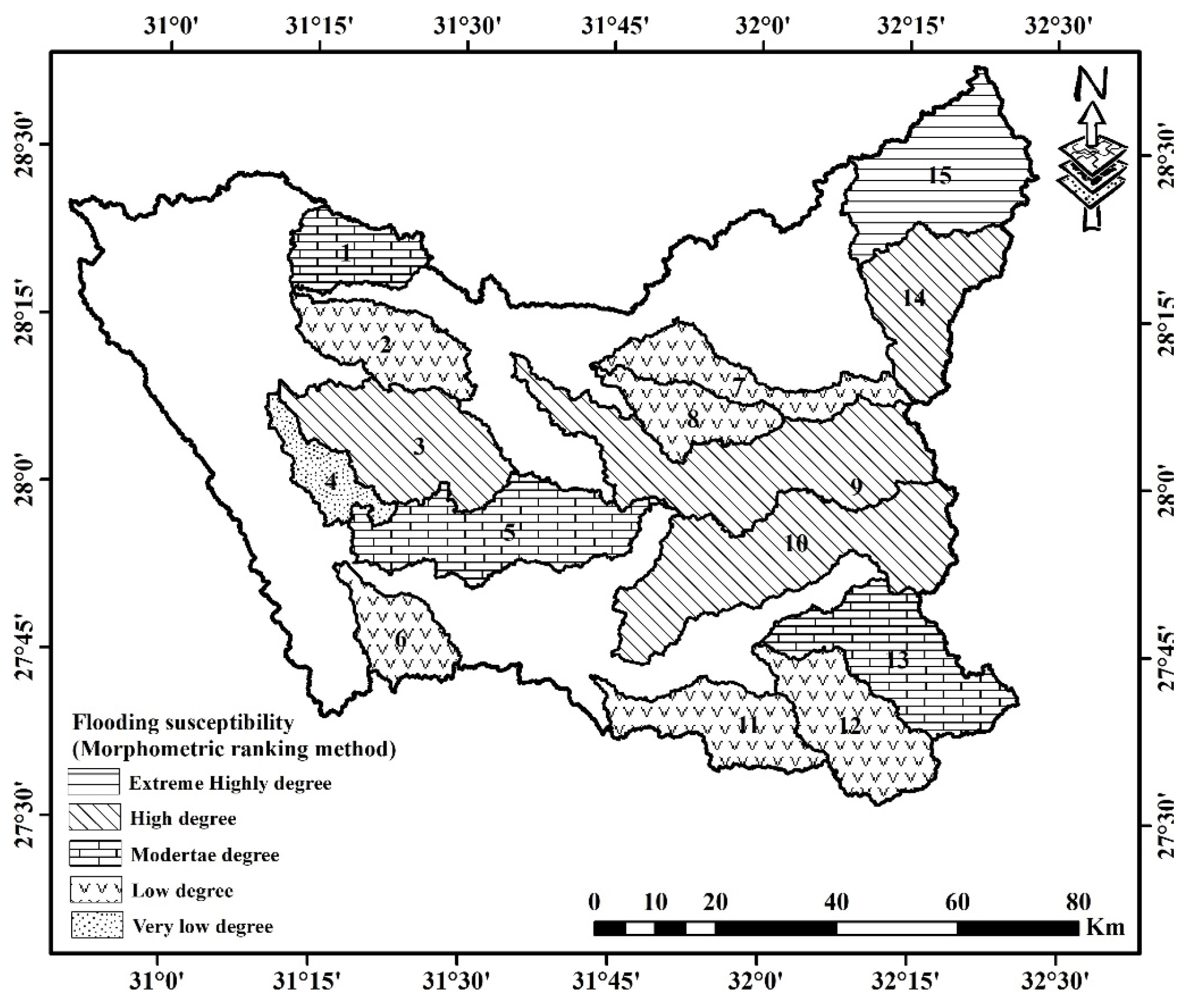
4.2. Flashflood Hazard Assessment
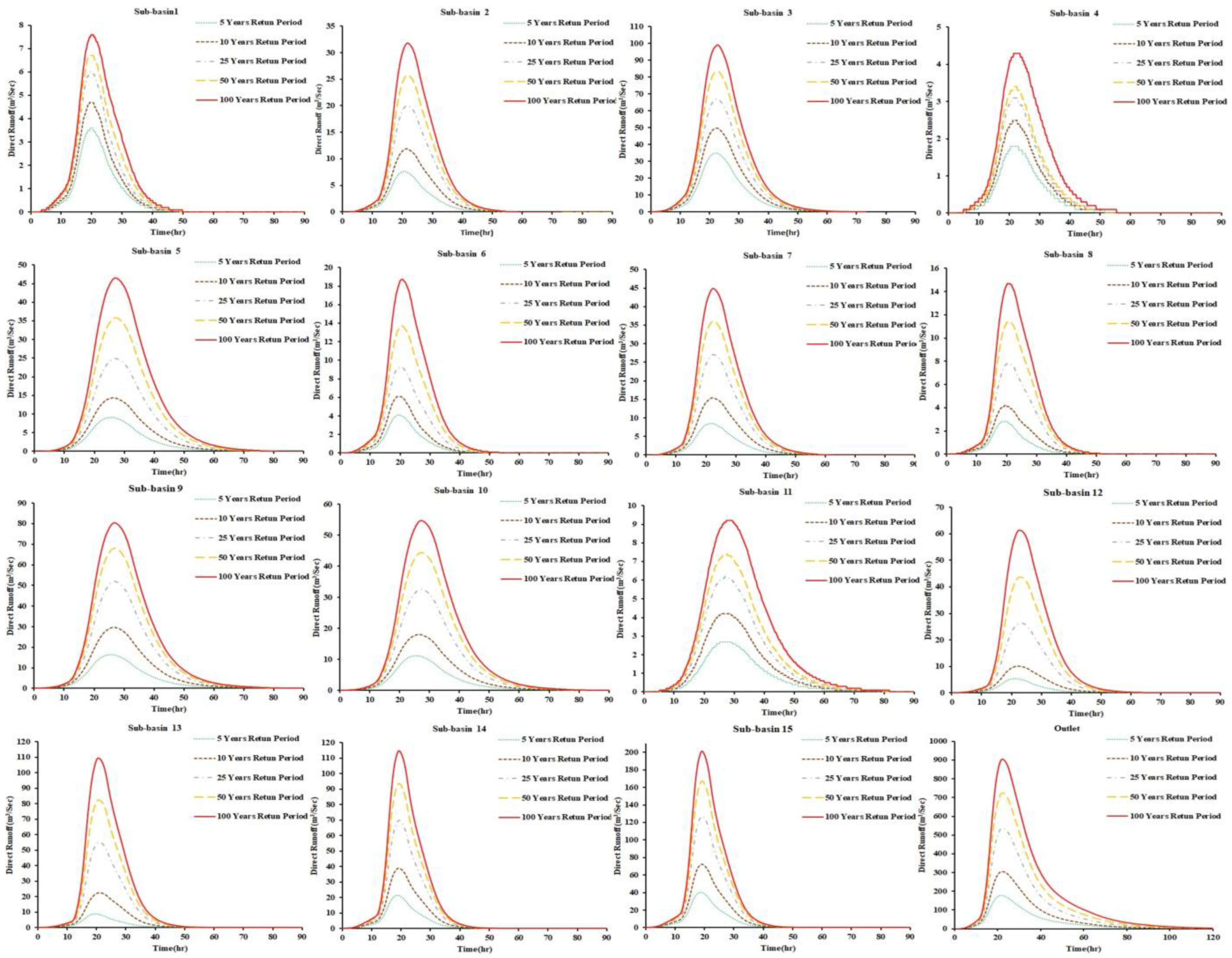
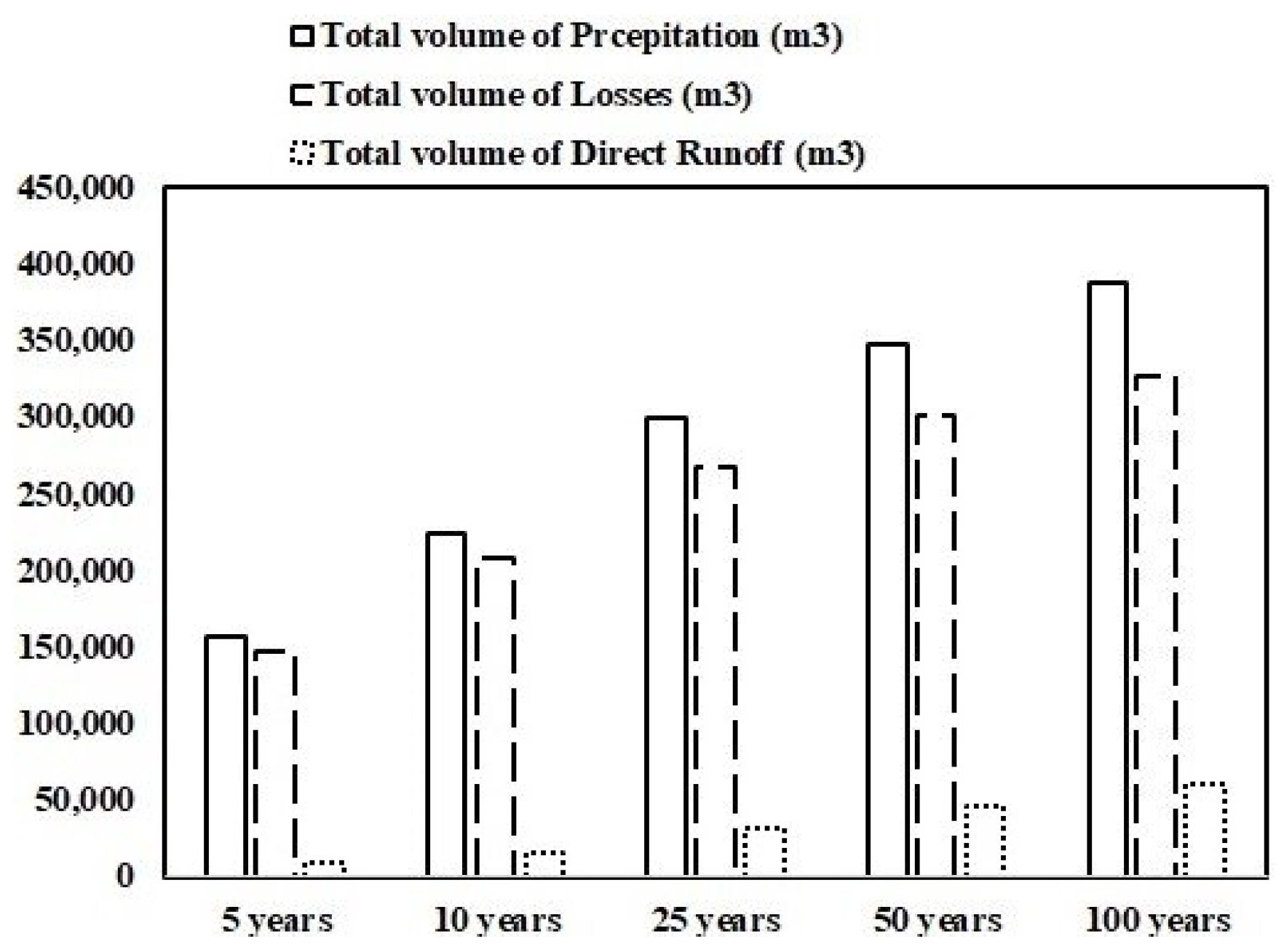
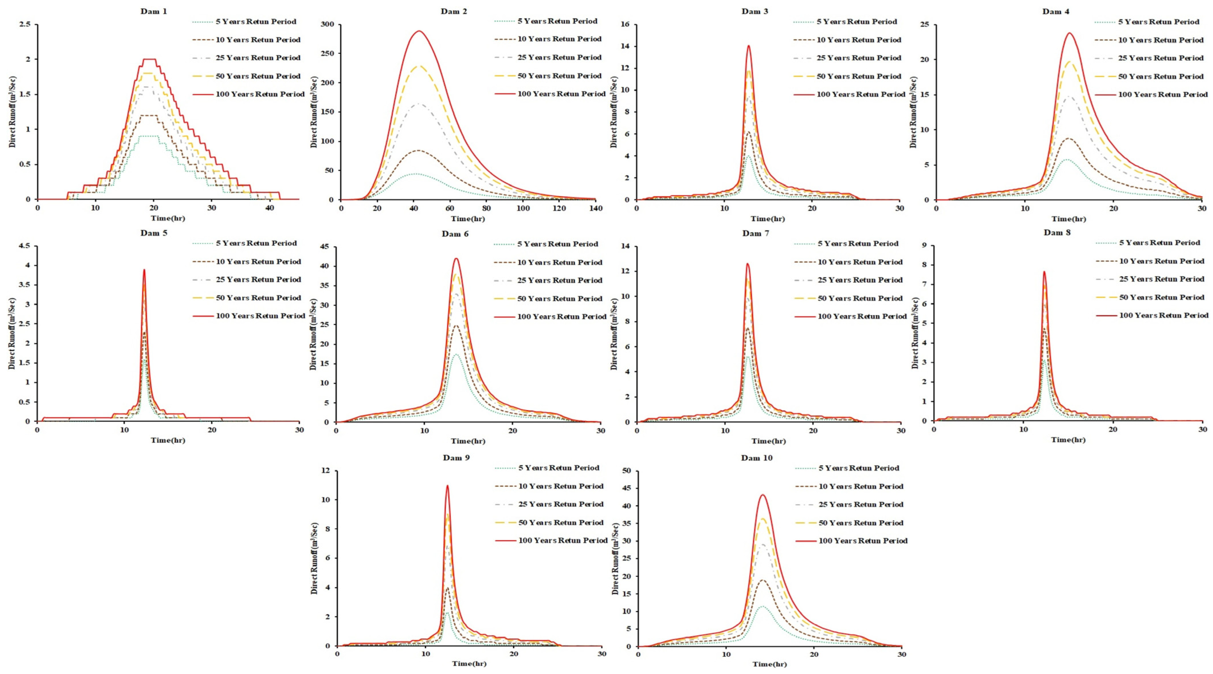
4.3. Rainfall–Runoff Modeling
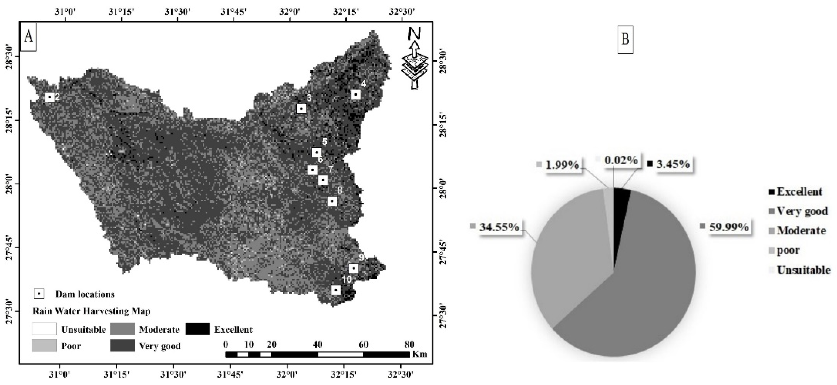
4.4. Multi-Criteria Decision Analysis for the Study Area
Rainfall-Harvesting Map
5. Conclusions
Author Contributions
Funding
Institutional Review Board Statement
Informed Consent Statement
Data Availability Statement
Acknowledgments
Conflicts of Interest
Appendix A

| ID | Lon(x) | Lat(y) | Begin | End | Max-Trend | Min-Trend | ||
|---|---|---|---|---|---|---|---|---|
| LinTrend/Decade | p-Value of t-Test | LinTrend/Decade | p-Value of t-Test | |||||
| N276313 | 31.25 | 27.632 | 1979 | 2014 | 0.270 | 0.018 | 0.210 | 0.037 |
| N276322 | 32.188 | 27.632 | 1979 | 2014 | 0.280 | 0.024 | 0.120 | 0.255 |
| N276325 | 32.5 | 27.632 | 1979 | 2014 | 0.370 | 0.002 | 0.160 | 0.075 |
| N279309 | 30.938 | 27.945 | 1979 | 2014 | 0.300 | 0.005 | 0.250 | 0.010 |
| N279313 | 31.25 | 27.945 | 1979 | 2014 | 0.270 | 0.015 | 0.180 | 0.075 |
| N279316 | 31.563 | 27.945 | 1979 | 2014 | 0.320 | 0.007 | 0.130 | 0.217 |
| N279319 | 31.875 | 27.945 | 1979 | 2014 | 0.370 | 0.002 | 0.130 | 0.212 |
| N279322 | 32.188 | 27.945 | 1979 | 2014 | 0.390 | 0.001 | 0.150 | 0.112 |
| N283309 | 30.938 | 28.257 | 1979 | 2014 | 0.340 | 0.001 | 0.420 | 0.001 |
| N283313 | 31.25 | 28.257 | 1979 | 2014 | 0.290 | 0.010 | 0.150 | 0.129 |
| N283316 | 31.563 | 28.257 | 1979 | 2014 | 0.310 | 0.008 | 0.040 | 0.735 |
| N283319 | 31.875 | 28.257 | 1979 | 2014 | 0.390 | 0.001 | 0.080 | 0.442 |
| N283322 | 32.188 | 28.257 | 1979 | 2014 | 0.430 | 0.000 | 0.040 | 0.686 |
| N286309 | 30.938 | 28.569 | 1979 | 2014 | 0.380 | 0.000 | 0.450 | 0.001 |
| N286313 | 31.25 | 28.569 | 1979 | 2014 | 0.280 | 0.010 | 0.100 | 0.317 |
| N286316 | 31.563 | 28.569 | 1979 | 2014 | 0.300 | 0.010 | −0.050 | 0.660 |
| N286319 | 31.875 | 28.569 | 1979 | 2014 | 0.420 | 0.001 | 0.040 | 0.723 |
| N286322 | 32.188 | 28.569 | 1979 | 2014 | 0.310 | 0.011 | −0.170 | 0.156 |
| N289309 | 30.94 | 28.88 | 1979 | 2014 | 0.340 | 0.001 | 0.360 | 0.002 |
| N289313 | 31.25 | 28.88 | 1979 | 2014 | 0.310 | 0.004 | −0.030 | 0.788 |
| N289316 | 31.56 | 28.88 | 1979 | 2014 | 0.410 | 0.000 | −0.010 | 0.923 |
| N289319 | 31.88 | 28.88 | 1979 | 2014 | 0.630 | 0.000 | 0.150 | 0.139 |
| N292313 | 31.250 | 29.193 | 1979 | 2014 | 0.390 | 0.000 | 0.050 | 0.566 |
| N292316 | 31.563 | 29.193 | 1979 | 2014 | 0.360 | 0.001 | 0.190 | 0.028 |
| N292319 | 31.875 | 29.193 | 1979 | 2014 | 0.400 | 0.000 | 0.190 | 0.026 |
| N295313 | 31.250 | 29.506 | 1979 | 2014 | 0.460 | 0.000 | 0.180 | 0.022 |
| N295316 | 31.563 | 29.506 | 1979 | 2014 | 0.440 | 0.000 | 0.280 | 0.002 |
| N295319 | 31.875 | 29.506 | 1979 | 2014 | 0.340 | 0.002 | 0.170 | 0.041 |
| ID | Lon(x) | Lat(y) | Begin | End | Precipitation Trend | Relative Humidity Trend | ||
|---|---|---|---|---|---|---|---|---|
| LinTrend/Decade | p-Value of t-Test | LinTrend/Decade | p-Value of t-Test | |||||
| N276313 | 31.25 | 27.632 | 1979 | 2014 | −8.520 | 0.015 | 0.000 | 0.000 |
| N276322 | 32.188 | 27.632 | 1979 | 2014 | −8.080 | 0.023 | −0.010 | 0.018 |
| N276325 | 32.5 | 27.632 | 1979 | 2014 | −7.110 | 0.025 | 0.000 | 0.092 |
| N279309 | 30.938 | 27.945 | 1979 | 2014 | −6.880 | 0.039 | 0.000 | 0.000 |
| N279313 | 31.25 | 27.945 | 1979 | 2014 | −5.730 | 0.068 | 0.000 | 0.000 |
| N279316 | 31.563 | 27.945 | 1979 | 2014 | −5.270 | 0.079 | 0.000 | 0.198 |
| N279319 | 31.875 | 27.945 | 1979 | 2014 | −5.100 | 0.085 | −0.010 | 0.054 |
| N279322 | 32.188 | 27.945 | 1979 | 2014 | −5.100 | 0.090 | 0.000 | 0.000 |
| N283309 | 30.938 | 28.257 | 1979 | 2014 | −5.080 | 0.107 | 0.000 | 0.000 |
| N283313 | 31.25 | 28.257 | 1979 | 2014 | −4.790 | 0.117 | 0.000 | 0.166 |
| N283316 | 31.563 | 28.257 | 1979 | 2014 | −4.690 | 0.158 | 0.000 | 0.000 |
| N283319 | 31.875 | 28.257 | 1979 | 2014 | −4.590 | 0.191 | 0.000 | 0.000 |
| N283322 | 32.188 | 28.257 | 1979 | 2014 | −3.990 | 0.205 | −0.010 | 0.295 |
| N286309 | 30.938 | 28.569 | 1979 | 2014 | −3.900 | 0.209 | −0.010 | 0.213 |
| N286313 | 31.25 | 28.569 | 1979 | 2014 | −3.900 | 0.215 | 0.010 | 0.147 |
| N286316 | 31.563 | 28.569 | 1979 | 2014 | −3.620 | 0.216 | 0.000 | 0.166 |
| N286319 | 31.875 | 28.569 | 1979 | 2014 | −3.530 | 0.239 | 0.000 | 0.638 |
| N286322 | 32.188 | 28.569 | 1979 | 2014 | −3.450 | 0.266 | −0.010 | 0.175 |
| N289309 | 30.94 | 28.88 | 1979 | 2014 | −3.300 | 0.269 | −0.010 | 0.444 |
| N289313 | 31.25 | 28.88 | 1979 | 2014 | −3.210 | 0.308 | 0.010 | 0.063 |
| N289316 | 31.56 | 28.88 | 1979 | 2014 | −2.500 | 0.360 | 0.000 | 0.498 |
| N289319 | 31.88 | 28.88 | 1979 | 2014 | −2.410 | 0.361 | −0.010 | 0.291 |
| N292313 | 31.250 | 29.193 | 1979 | 2014 | −2.230 | 0.384 | 0.000 | 0.166 |
| N292316 | 31.563 | 29.193 | 1979 | 2014 | −2.220 | 0.387 | 0.000 | 0.166 |
| N292319 | 31.875 | 29.193 | 1979 | 2014 | −2.180 | 0.473 | −0.010 | 0.152 |
| N295313 | 31.250 | 29.506 | 1979 | 2014 | −1.740 | 0.519 | −0.010 | 0.161 |
| N295316 | 31.563 | 29.506 | 1979 | 2014 | −1.510 | 0.574 | −0.020 | 0.059 |
| N295319 | 31.875 | 29.506 | 1979 | 2014 | −0.740 | 0.773 | −0.010 | 0.072 |
| ID | Lon(x) | Lat(y) | Begin | End | Sunshine Trend | Wind Trend | ||
|---|---|---|---|---|---|---|---|---|
| LinTrend/Decade | p-Value of t-Test | Amount/Decade | Sig. Level | |||||
| N276313 | 31.25 | 27.632 | 1979 | 2014 | 0.180 | 0.005 | −0.030 | 0.084 |
| N276322 | 32.188 | 27.632 | 1979 | 2014 | 0.190 | 0.004 | −0.060 | 0.005 |
| N276325 | 32.5 | 27.632 | 1979 | 2014 | 0.200 | 0.003 | −0.090 | 0.002 |
| N279309 | 30.938 | 27.945 | 1979 | 2014 | 0.230 | 0.001 | −0.020 | 0.088 |
| N279313 | 31.25 | 27.945 | 1979 | 2014 | 0.180 | 0.004 | −0.020 | 0.048 |
| N279316 | 31.563 | 27.945 | 1979 | 2014 | 0.150 | 0.013 | −0.050 | 0.004 |
| N279319 | 31.875 | 27.945 | 1979 | 2014 | 0.150 | 0.014 | −0.070 | 0.000 |
| N279322 | 32.188 | 27.945 | 1979 | 2014 | 0.210 | 0.003 | −0.070 | 0.002 |
| N283309 | 30.938 | 28.257 | 1979 | 2014 | 0.240 | 0.001 | −0.010 | 0.387 |
| N283313 | 31.25 | 28.257 | 1979 | 2014 | 0.200 | 0.004 | −0.010 | 0.323 |
| N283316 | 31.563 | 28.257 | 1979 | 2014 | 0.170 | 0.009 | −0.040 | 0.006 |
| N283319 | 31.875 | 28.257 | 1979 | 2014 | 0.170 | 0.008 | −0.060 | 0.002 |
| N283322 | 32.188 | 28.257 | 1979 | 2014 | 0.220 | 0.003 | −0.070 | 0.001 |
| N286309 | 30.938 | 28.569 | 1979 | 2014 | 0.240 | 0.001 | 0.010 | 0.528 |
| N286313 | 31.25 | 28.569 | 1979 | 2014 | 0.180 | 0.005 | −0.010 | 0.213 |
| N286316 | 31.563 | 28.569 | 1979 | 2014 | 0.160 | 0.009 | −0.050 | 0.001 |
| N286319 | 31.875 | 28.569 | 1979 | 2014 | 0.190 | 0.005 | −0.050 | 0.001 |
| N286322 | 32.188 | 28.569 | 1979 | 2014 | 0.240 | 0.002 | −0.080 | 0.000 |
| N289309 | 30.94 | 28.88 | 1979 | 2014 | 0.240 | 0.001 | 0.000 | 0.883 |
| N289313 | 31.25 | 28.88 | 1979 | 2014 | 0.170 | 0.007 | −0.020 | 0.063 |
| N289316 | 31.56 | 28.88 | 1979 | 2014 | 0.170 | 0.011 | −0.060 | 0.001 |
| N289319 | 31.88 | 28.88 | 1979 | 2014 | 0.210 | 0.003 | −0.060 | 0.000 |
| N292313 | 31.250 | 29.193 | 1979 | 2014 | 0.200 | 0.003 | −0.020 | 0.095 |
| N292316 | 31.563 | 29.193 | 1979 | 2014 | 0.210 | 0.002 | −0.040 | 0.005 |
| N292319 | 31.875 | 29.193 | 1979 | 2014 | 0.240 | 0.002 | −0.060 | 0.000 |
| N295313 | 31.250 | 29.506 | 1979 | 2014 | 0.250 | 0.001 | −0.010 | 0.281 |
| N295316 | 31.563 | 29.506 | 1979 | 2014 | 0.250 | 0.001 | −0.030 | 0.004 |
| N295319 | 31.875 | 29.506 | 1979 | 2014 | 0.260 | 0.001 | −0.040 | 0.004 |
| Morphometric Parameters | Formula | Reference |
|---|---|---|
| Stream order (U) | Hierarchical order | [1] |
| Stream Length (LU) km | The total length of the stream of order (u) | [2] |
| Bifurcation Ratio (Rb) | Rb = Nu/Nu + 1, where Nu = number of stream segments in order | [3] |
| (u), Nu + 1 = number of segments of the next higher order | ||
| Mean bifurcation ratio (MRb) | The average of bifurcation ratios of all orders | [1] |
| Weighted Mean bifurcation ratio (WMRb) | WMRb = Σ (Nu/Nu + 1)/ × (Nu + Nu + 1) N Where Nu = number of stream segments in order | [4] |
| (u), Nu+1 = number of segments of the next higher | ||
| order, N = total number of streams involved | ||
| Basin length (Lb) km | Extracted by the spatial analyst tool in ArcMap | [3] |
| Length of overland flow (Lg) km | Lg = 1/2 Dd, where Dd = drainage density | [2] |
| Morphometric Parameters | Formula | Reference |
|---|---|---|
| Basin area (A) km2 | Extracted by the spatial analyst tool in ArcMap | [3] |
| Basin perimeter (P) km | Extracted by the spatial analyst tool in ArcMap | [3] |
| Drainage density (Dd) km/km2 | Dd = L/A, where L = total length of the stream, | [5] |
| A = area of the basin | ||
| Stream frequency (Fs) km−2 | Fs = ΣN/A, where ΣN = total number of stream segments in all orders, A = area of the basin | [5] |
| Texture ratio (T) | T = ΣN/P, where ΣN = Total number of stream segments in all orders, P = perimeter of the basin | [2] |
| Shape index (Ish) | Ish = 1.27 × Rf (Rf form factor) | [2,3] |
| Morphometric Parameters | Formula | Reference |
|---|---|---|
| Relief ratio (Rh) | Rh = Bh/Lb, where Bh = basin relief, Lb = basin length | [3] |
| Basin slope (BS) | Extracted by (WMS software) | [2] |
| Drainage patterns (Dp) | Stream network using GIS software analysis | [5] |
| Ruggedness Number (Rn) | Rn = Bh × Dd, where Bh = basin relief, Dd = drainage density | [6] |
| Slope index (SI) | SI = Bh/Lms, where Bh = basin relief, Lms = length of main stream | [7] |
| Intensity of Importance | Definition | Description |
|---|---|---|
| 1 | Equally important | Two factors contribute equally to the objective. |
| 3 | Moderately more important | Experience and judgment slightly favor one over the other. |
| 5 | Strongly more important | Experience and judgment strongly favor one over the other. |
| 7 | Very strongly more important | Experience and judgment very strongly favor one over the other. Its importance is demonstrated in practice. |
| 9 | Extremely more important | The evidence favoring one over the other is of the highest possible validity. |
| 2, 4, 6, 8 | Intermediate values | When compromise was needed |
Appendix B


Appendix C
| Basin No | U | 1 | 2 | 3 | 4 | 5 | 6 | 7 | 8 | 9 |
|---|---|---|---|---|---|---|---|---|---|---|
| 1 | Nu | 2625 | 652 | 140 | 29 | 8 | 3 | 1 | ||
| Lu (km) | 556.29 | 275.67 | 149.07 | 82.28 | 56.47 | 13.16 | 7.12 | |||
| 2 | Nu | 3505 | 877 | 172 | 41 | 11 | 2 | 1 | ||
| Lu (km) | 776.29 | 382.13 | 194.00 | 110.30 | 51.87 | 27.41 | 8.80 | |||
| 3 | Nu | 5993 | 1997 | 362 | 80 | 16 | 6 | 1 | ||
| Lu (km) | 1348.86 | 669.64 | 318.08 | 168.54 | 81.74 | 37.71 | 33.26 | |||
| 4 | Nu | 1843 | 519 | 123 | 24 | 5 | 2 | 1 | ||
| Lu (km) | 434.04 | 222.36 | 85.16 | 42.72 | 28.17 | 11.98 | 12.39 | |||
| 5 | Nu | 6376 | 2034 | 543 | 73 | 15 | 4 | 1 | ||
| Lu (km) | 1430.07 | 669.93 | 348.81 | 182.92 | 89.67 | 30.04 | 39.11 | |||
| 6 | Nu | 2447 | 604 | 138 | 36 | 8 | 2 | 1 | ||
| Lu (km) | 577.43 | 257.21 | 144.54 | 65.79 | 18.14 | 22.07 | 12.21 | |||
| 7 | Nu | 3344 | 733 | 143 | 22 | 7 | 2 | 1 | ||
| Lu (km) | 699.06 | 326.43 | 163.55 | 62.02 | 56.98 | 42.07 | 10.49 | |||
| 8 | Nu | 2676 | 676 | 178 | 26 | 5 | 2 | 1 | ||
| Lu (km) | 549.64 | 244.73 | 155.16 | 54.20 | 53.85 | 5.80 | 11.42 | |||
| 9 | Nu | 9213 | 2300 | 354 | 93 | 15 | 5 | 1 | ||
| Lu (km) | 1994.32 | 894.01 | 437.24 | 211.35 | 125.83 | 65.09 | 75.56 | |||
| 10 | Nu | 9446 | 2123 | 386 | 90 | 22 | 4 | 1 | ||
| Lu (km) | 2023.56 | 901.20 | 401.82 | 242.77 | 140.58 | 48.76 | 59.62 | |||
| 11 | Nu | 3934 | 813 | 168 | 38 | 9 | 2 | 1 | ||
| Lu (km) | 833.14 | 359.14 | 178.75 | 102.65 | 51.98 | 23.56 | 19.43 | |||
| 12 | Nu | 4663 | 871 | 191 | 38 | 9 | 2 | 1 | ||
| Lu (km) | 972.49 | 440.32 | 206.93 | 114.37 | 66.52 | 34.78 | 7.63 | |||
| 13 | Nu | 5612 | 921 | 236 | 55 | 12 | 3 | 1 | ||
| Lu (km) | 1176.75 | 540.18 | 269.20 | 137.82 | 87.75 | 16.95 | 29.10 | |||
| 14 | Nu | 4553 | 881 | 204 | 54 | 12 | 3 | 1 | ||
| Lu (km) | 996.85 | 490.41 | 250.82 | 121.25 | 68.16 | 33.02 | 11.84 | |||
| 15 | Nu | 6427 | 1121 | 299 | 72 | 16 | 4 | 1 | ||
| Lu (km) | 1379.75 | 650.98 | 302.15 | 170.50 | 104.58 | 22.70 | 39.71 | |||
| Main basin | Nu | 125,068 | 29,081 | 6835 | 1225 | 279 | 70 | 15 | 3 | 1 |
| Lu (km) | 27,120.47 | 12,688.2 | 6344 | 3193 | 1672.78 | 772.08 | 382.19 | 393 | 11.08 |
| Basin No | U | MRb | WMRb | Lb | Lg |
|---|---|---|---|---|---|
| 1 | 7 | 3.80 | 4.17 | 23.80 | 2.55 |
| 2 | 7 | 4.09 | 4.21 | 34.57 | 2.56 |
| 3 | 7 | 4.35 | 3.67 | 41.87 | 2.60 |
| 4 | 7 | 3.70 | 3.77 | 28.99 | 2.63 |
| 5 | 7 | 8.98 | 3.55 | 52.91 | 2.57 |
| 6 | 7 | 3.79 | 4.11 | 27.02 | 2.66 |
| 7 | 7 | 4.14 | 4.71 | 53.65 | 2.43 |
| 8 | 7 | 4.05 | 4.08 | 33.39 | 2.41 |
| 9 | 7 | 4.75 | 4.49 | 73.56 | 2.43 |
| 10 | 7 | 4.64 | 4.63 | 63.09 | 2.42 |
| 11 | 7 | 4.14 | 4.82 | 41.63 | 2.45 |
| 12 | 7 | 4.28 | 5.21 | 37.16 | 2.37 |
| 13 | 7 | 4.31 | 5.72 | 44.26 | 2.30 |
| 14 | 7 | 4.13 | 4.98 | 32.49 | 2.50 |
| 15 | 7 | 4.36 | 5.38 | 39.63 | 2.41 |
| Main basin | 9 | 4.40 | 4.35 | 177.72 | 2.47 |
| Basin No | A | P | Dd | Fs | T | Rh | BS | Dp |
|---|---|---|---|---|---|---|---|---|
| 1 | 223.79 | 93.66 | 5.09 | 15.45 | 36.92 | 0.0105 | 0.0615 | Dendritic |
| 2 | 302.86 | 113.17 | 5.12 | 15.22 | 40.72 | 0.0060 | 0.0411 | Dendritic |
| 3 | 511.88 | 151.73 | 5.19 | 16.52 | 54.17 | 0.0063 | 0.0473 | Dendritic |
| 4 | 159.01 | 103.37 | 5.26 | 15.83 | 24.35 | 0.0046 | 0.0413 | Dendritic |
| 5 | 543.16 | 196.98 | 5.14 | 16.65 | 45.92 | 0.0059 | 0.0406 | Dendritic |
| 6 | 206.29 | 90.08 | 5.32 | 15.69 | 35.93 | 0.0048 | 0.0419 | Dendritic |
| 7 | 280.38 | 157.98 | 4.85 | 15.17 | 26.91 | 0.0098 | 0.0684 | Dendritic |
| 8 | 222.95 | 103.91 | 4.82 | 15.99 | 34.30 | 0.0090 | 0.0703 | Dendritic |
| 9 | 783.91 | 258.93 | 4.85 | 15.28 | 46.27 | 0.0083 | 0.0664 | Dendritic |
| 10 | 789.01 | 221.50 | 4.84 | 15.30 | 54.50 | 0.0084 | 0.0629 | Dendritic |
| 11 | 320.00 | 132.89 | 4.90 | 15.52 | 37.36 | 0.0066 | 0.0457 | Dendritic |
| 12 | 389.19 | 120.16 | 4.74 | 14.84 | 48.06 | 0.0074 | 0.0599 | Dendritic |
| 13 | 490.33 | 150.54 | 4.60 | 13.95 | 45.44 | 0.0088 | 0.1028 | Dendritic |
| 14 | 393.99 | 117.86 | 5.01 | 14.49 | 48.43 | 0.0126 | 0.0652 | Dendritic |
| 15 | 553.10 | 147.26 | 4.83 | 14.36 | 53.92 | 0.0171 | 0.1145 | Dendritic |
| Main basin | 10646.40 | 807.59 | 4.94 | 15.27 | 201.31 | 0.0070 | 0.0556 | Dendritic |
| Basin No | A (km2) | ΣA × CN | CNw | S (in) | Ia (in) | BS% | FL (ft) | TL (h) | TC (h) |
|---|---|---|---|---|---|---|---|---|---|
| 1 | 223 | 15,933.44 | 71.22 | 4.04 | 0.81 | 6.15 | 72,377.15 | 5.08 | 8.47 |
| 2 | 302 | 25,157.41 | 83.07 | 2.04 | 0.41 | 4.11 | 119,060.67 | 6.50 | 10.83 |
| 3 | 511 | 42,278.18 | 82.59 | 2.11 | 0.42 | 4.73 | 178,378.32 | 8.50 | 14.17 |
| 4 | 159 | 11,413.72 | 71.77 | 3.93 | 0.79 | 4.13 | 121,821.39 | 9.27 | 15.45 |
| 5 | 543 | 44,544.76 | 82.01 | 2.19 | 0.44 | 4.06 | 204,723.68 | 10.44 | 17.41 |
| 6 | 206 | 15,924.80 | 77.19 | 2.96 | 0.59 | 4.19 | 94,069.65 | 6.41 | 10.68 |
| 7 | 280 | 23,276.96 | 83.01 | 2.05 | 0.41 | 6.84 | 260,557.45 | 9.44 | 15.74 |
| 8 | 222 | 17,573.92 | 78.83 | 2.69 | 0.54 | 7.03 | 150,120.48 | 6.85 | 11.41 |
| 9 | 783 | 64,419.36 | 82.18 | 2.17 | 0.43 | 6.64 | 356,437.61 | 12.66 | 21.10 |
| 10 | 789 | 62,472.33 | 79.18 | 2.63 | 0.53 | 6.29 | 271,505.66 | 11.50 | 19.17 |
| 11 | 319 | 20,926.63 | 65.40 | 5.29 | 1.06 | 4.57 | 160,659.67 | 13.03 | 21.72 |
| 12 | 389 | 30,302.01 | 77.87 | 2.84 | 0.57 | 5.99 | 160,031.35 | 8.04 | 13.40 |
| 13 | 490 | 40,018.41 | 81.63 | 2.25 | 0.45 | 10.28 | 206,709.81 | 6.70 | 11.16 |
| 14 | 393 | 31,334.85 | 79.54 | 2.57 | 0.51 | 6.52 | 71,064.32 | 3.82 | 6.37 |
| 15 | 553 | 43,916.03 | 79.40 | 2.59 | 0.52 | 11.45 | 164,929.31 | 5.68 | 9.47 |
| Mainbasin | 10,646 | 829,384.58 | 77.90 | 2.84 | 0.57 | 5.56 | 765,364.20 | 29.14 | 48.57 |
| Decision Factors at Level 2 (i) | Relative Weight at Level 2 of Decision Factor i = RIW2 i | Decision Sub-Factors (j) at Level 3 (Cell Attribute) | Ranking Decision |
|---|---|---|---|
| Land-cover units | 0.2085 | Vegetation | 1 |
| Recent Alluvial | 2 | ||
| Old Alluvial | 3 | ||
| Quarries | 4 | ||
| Limestone with clay | 5 | ||
| Massive limestone | 6 | ||
| Average of max 24 h rainfall depth (mm) | 0.1852 | 5.875200748–6.75068903 | 1 |
| 6.750689031–7.658358574 | 2 | ||
| 7.658358575–9.030816078 | 3 | ||
| 9.030816079–10.76387215 | 4 | ||
| 10.76387216–12.63123417 | 5 | ||
| Slope (degrees) | 0.477 | 0–2.764199904 | 5 |
| 2.764199905–5.74103057 | 4 | ||
| 5.741030571–10.41890733 | 3 | ||
| 10.41890734–18.28624552 | 2 | ||
| 18.28624553–54.00821351 | 1 | ||
| Stream order | 0.0592 | 1 | 1 |
| 2 | 2 | ||
| 3 | 3 | ||
| 4 | 4 | ||
| 5 | 5 | ||
| 6 | 6 | ||
| 7 | 7 | ||
| 8 | 8 | ||
| 9 | 9 | ||
| Lineaments density (km/km2) | 0.0701 | 0–0.206917985 | 5 |
| 0.206917985–0.389492678 | 4 | ||
| 0.389492678–0.614668133 | 3 | ||
| 0.614668133–0.912873465 | 2 | ||
| 0.912873465–1.55188489 | 1 |
| Basin No | A (km2) | ΣA × CN | CNw | S (in) | Ia (in) | BS% | FL (ft) | TL (h) | TC (h) |
|---|---|---|---|---|---|---|---|---|---|
| 1 | 52.98 | 3670.83 | 69.29 | 4.43 | 0.89 | 3.80 | 63,692.77 | 6.15 | 10.26 |
| 2 | 4747.77 | 379,441.81 | 79.92 | 2.51 | 0.50 | 5.91 | 729,000.85 | 25.56 | 42.60 |
| 3 | 7.53 | 642.97 | 85.44 | 1.70 | 0.34 | 10.72 | 18,217.73 | 0.83 | 1.38 |
| 4 | 39.07 | 3002.85 | 76.85 | 3.01 | 0.60 | 9.40 | 52,865.40 | 2.73 | 4.54 |
| 5 | 0.85 | 75.43 | 88.41 | 1.31 | 0.26 | 7.40 | 3026.79 | 0.21 | 0.35 |
| 6 | 22.17 | 1935.19 | 87.29 | 1.46 | 0.29 | 7.11 | 30,812.99 | 1.44 | 2.41 |
| 7 | 4.27 | 367.02 | 85.98 | 1.63 | 0.33 | 10.67 | 15,192.13 | 0.70 | 1.17 |
| 8 | 2.12 | 182.83 | 86.37 | 1.58 | 0.32 | 8.45 | 6726.45 | 0.41 | 0.68 |
| 9 | 3.99 | 335.43 | 84.15 | 1.88 | 0.38 | 15.91 | 12,422.02 | 0.52 | 0.87 |
| 10 | 23.01 | 1936.89 | 84.16 | 1.88 | 0.38 | 6.21 | 37,567.51 | 2.02 | 3.37 |
| Dam No | Max Elevation (m) | Max Height (m) | Max Storage capacity (m3) | Max surface area (m2) |
|---|---|---|---|---|
| 1 | 107 | 24 | 2,653,602.08 | 291,793.19 |
| 2 | 103 | 23 | 10,720,852.86 | 1,489,698.49 |
| 3 | 565 | 20 | 1,629,981.86 | 296,494.06 |
| 4 | 693 | 18 | 1,189,841.62 | 154,441.31 |
| 5 | 705 | 17 | 1,107,544.42 | 157,873.34 |
| 6 | 660 | 18 | 3,421,759.67 | 501,554.30 |
| 7 | 711 | 19 | 2,716,737.12 | 295,154.51 |
| 8 | 740 | 22 | 4,905,677.69 | 581,781.67 |
| 9 | 710 | 22 | 2,277,794.88 | 261,692.23 |
| 10 | 650 | 20 | 2,411,787.02 | 284,858.42 |
References
- Costa, J.E. Hydraulics and Basin Morphometry of the Largest Flash Floods in the Conterminous United States. J Hydrol. 1987, 93, 313–338. [Google Scholar] [CrossRef]
- He, B.; Huang, X.; Ma, M.; Chang, Q.; Tu, Y.; Li, Q.; Zhang, K.; Hong, Y. Analysis of Flash Flood Disaster Characteristics in China from 2011 to 2015. Nat. Hazards 2018, 90, 407–420. [Google Scholar] [CrossRef]
- Abdalla, F.; Shamy, I.E.; Bamousa, A.O.; Mansour, A.; Mohamed, A.; Tahoon, M. Flash Floods and Groundwater Recharge Potentials in Arid Land Alluvial Basins, Southern Red Sea Coast, Egypt. Int. J. Geosci. 2014, 5, 971–982. [Google Scholar] [CrossRef] [Green Version]
- Davies, R. World Disasters Report—Most Deaths Caused by Floods. 2014. Available online: https://floodlist.com/dealing-with-floods/world-disasters-report-100-million-affected-2013 (accessed on 15 October 2022).
- Dano, U.L. Flash Flood Impact Assessment in Jeddah City: An Analytic Hierarchy Process Approach. Hydrology 2020, 7, 10. [Google Scholar] [CrossRef] [Green Version]
- Prama, M.; Omran, A.; Schröder, D.; Abouelmagd, A. Vulnerability Assessment of Flash Floods in Wadi Dahab Basin, Egypt. Env. Earth Sci. 2020, 79, 1–17. [Google Scholar] [CrossRef] [Green Version]
- Lin, X. Flash Floods in Arid and Semi-Arid Zones. Tech. Doc. Hydrol. 1999. Available online: https://unesdoc.unesco.org/ark:/48223/pf0000118882 (accessed on 15 October 2022).
- Youssef, A.M.; Pradhan, B.; Hassan, A.M. Flash Flood Risk Estimation along the St. Katherine Road, Southern Sinai, Egypt Using GIS Based Morphometry and Satellite Imagery. Environ. Earth Sci. 2011, 62, 611–623. [Google Scholar] [CrossRef]
- Moawad, M.B.; Aziz, A.O.A.; Mamtimin, B. Flash Floods in the Sahara: A Case Study for the 28 January 2013 Flood in Qena, Egypt. Geomat. Nat. Hazards Risk 2016, 7, 215–236. [Google Scholar] [CrossRef] [Green Version]
- Abdelkader, M.M.; Al-Amoud, A.I.; El-Alfy, M.; El-Feky, A.; Saber, M. Assessment of Flash Flood Hazard Based on Morphometric Aspects and Rainfall-Runoff Modeling in Wadi Nisah, Central Saudi Arabia. Remote Sens. Appl. 2021, 23, 100562. [Google Scholar] [CrossRef]
- Elsebaie, I.H.; el Alfy, M.; Kawara, A.Q. Spatiotemporal Variability of Intensity–Duration–Frequency (IDF) Curves in Arid Areas: Wadi AL-Lith, Saudi Arabia as a Case Study. Hydrology 2021, 9, 6. [Google Scholar] [CrossRef]
- Tizro, A.T.; Voudouris, K.S.; Akbari, K. Simulation of a Groundwater Artificial Recharge in a Semi-Arid Region of Iran. Irrig. Drain. 2011, 60, 393–403. [Google Scholar] [CrossRef]
- Sarma, D.; Xu, Y. The Recharge Process in Alluvial Strip Aquifers in Arid Namibia and Implication for Artificial Recharge. Hydrogeology 2017, 25, 123–134. [Google Scholar] [CrossRef]
- Alataway, A.; El-Alfy, M. Rainwater Harvesting and Artificial Groundwater Recharge in Arid Areas: Case Study in Wadi Al-Alb, Saudi Arabia. J. Water Resour. Plan. Manag. 2019, 145, 05018017. [Google Scholar] [CrossRef]
- Sturm, M.; Zimmermann, M.; Schütz, K.; Urban, W.; Hartung, H. Rainwater Harvesting as an Alternative Water Resource in Rural Sites in Central Northern Namibia. Phys. Chem. Earth Parts A/B/C 2009, 34, 776–785. [Google Scholar] [CrossRef]
- El-Alfy, M. Applications of Engineering Geology on the Geomorphological and Hydrogeological Situations of the Area between Rafah and Ras El-Naqab. Master’s Thesis, Mansoura University, Mansoura, Egypt, 1998. [Google Scholar]
- Escalante, E.F.; Gil, R.C.; Fraile, M.Á.S.M.; Serrano, F.S. Economic Assessment of Opportunities for Managed Aquifer Recharge Techniques in Spain Using an Advanced Geographic Information System (GIS). Water 2014, 6, 2021–2040. [Google Scholar] [CrossRef] [Green Version]
- Qi, Q.; Marwa, J.; Mwamila, T.B.; Gwenzi, W.; Noubactep, C. Making Rainwater Harvesting a Key Solution for Water Management: The Universality of the Kilimanjaro Concept. Sustainability 2019, 11, 5606. [Google Scholar] [CrossRef] [Green Version]
- Ammar, A.; Riksen, M.; Ouessar, M.; Ritsema, C. Identification of Suitable Sites for Rainwater Harvesting Structures in Arid and Semi-Arid Regions: A Review. Int. Soil Water Conserv. Res. 2016, 4, 108–120. [Google Scholar] [CrossRef] [Green Version]
- Musaed, H.A.H.; Al-Bassam, A.M.; Zaidi, F.K.; Alfaifi, H.J.; Ibrahim, E. Hydrochemical Assessment of Groundwater in Mesozoic Sedimentary Aquifers in an Arid Region: A Case Study from Wadi Nisah in Central Saudi Arabia. Environ. Earth Sci. 2020, 79, 1–12. [Google Scholar] [CrossRef]
- El-Alfy, M.; Merkel, B. Hydrochemical Relationships and Geochemical Modeling of Ground Water in Al Arish Area, North Sinai, Egypt. Hydrol. Sci. Technol. 2006, 22, 47–62. [Google Scholar]
- El-Alfy, M. Hydrochemical Modeling and Assessment of Groundwater Contamination in Northwest Sinai, Egypt. Water Environ. Res. 2013, 85, 211–223. [Google Scholar] [CrossRef]
- Mahmoud, S.H.; Alazba, A.A.; Adamowski, J.; El-Gindy, A.M. GIS Methods for Sustainable Stormwater Harvesting and Storage Using Remote Sensing for Land Cover Data—Location Assessment. Environ. Monit. Assess. 2015, 187, 1–19. [Google Scholar] [CrossRef]
- Balkhair, K.S.; Ur Rahman, K. Development and Assessment of Rainwater Harvesting Suitability Map Using Analytical Hierarchy Process, GIS and RS Techniques. Geocarto. Int. 2021, 36, 421–448. [Google Scholar] [CrossRef]
- Ouali, L.; Hssaisoune, M.; Kabiri, L.; Slimani, M.M.; el Mouquaddam, K.; Namous, M.; Arioua, A.; ben Moussa, A.; Benqlilou, H.; Bouchaou, L. Mapping of Potential Sites for Rainwater Harvesting Structures Using GIS and MCDM Approaches: Case Study of the Toudgha Watershed, Morocco. EuroMediterr. J. Env. Integr. 2022, 7, 49–64. [Google Scholar] [CrossRef]
- El-Magd, S.A.A.; Pradhan, B.; Alamri, A. Machine Learning Algorithm for Flash Flood Prediction Mapping in Wadi El-Laqeita and Surroundings, Central Eastern Desert, Egypt. Arab. J. Geosci. 2021, 14, 1–14. [Google Scholar] [CrossRef]
- Taha, M.M.N.; Elbarbary, S.M.; Naguib, D.M.; El-Shamy, I.Z. Flash Flood Hazard Zonation Based on Basin Morphometry Using Remote Sensing and GIS Techniques: A Case Study of Wadi Qena Basin, Eastern Desert, Egypt. Remote Sens. Appl. 2017, 8, 157–167. [Google Scholar] [CrossRef]
- El-Bastawesy, M.; Abu El Ella, E.M. Quantitative Estimates of Flash Flood Discharge into Waste Water Disposal Sites in Wadi Al Saaf, the Eastern Desert of Egypt. J. Afr. Earth Sci. 2017, 136, 312–318. [Google Scholar] [CrossRef]
- Abbas, M.; Carling, P.A.; Jansen, J.D.; Al-Saqarat, B.S. Flash-Flood Hydrology and Aquifer-Recharge in Wadi Umm Sidr, Eastern Desert, Egypt. J. Arid Environ. 2020, 178, 104170. [Google Scholar] [CrossRef]
- Harmsen, J. A New and Scalable Approach for Rural Sanitation in Egypt: The Deir Gabal El-Tair Pilot. The Environmental Technology for Impact Conference (ETEI2015). 2016. Available online: https://scholar.google.com/scholar?hl=en&as_sdt=0%2C5&q=A+New+and+Scalable+Approach+for+Rural+Sanitation+in+Egypt%3A+The+Deir+Gabal+El-Tair+Pilot&btnG= (accessed on 15 October 2022).
- Khalil, M.; Abotalib, A.; Farag, M.; Rabei, M.; Abdelhady, A.A.; Pichler, T. Poor Drainage-Induced Waterlogging in Saharan Groundwater-Irrigated Lands: Integration of Geospatial, Geophysical, and Hydrogeological Techniques. Catena 2021, 207, 105615. [Google Scholar] [CrossRef]
- Moneim, A.A.A. Overview of the Geomorphological and Hydrogeological Characteristics of the Eastern Desert of Egypt. Hydrogeol. J. 2005, 13, 416–425. [Google Scholar] [CrossRef]
- El-Saadawy, O.; Gaber, A.; Othman, A.; Abotalib, A.Z.; Bastawesy, M.E.; Attwa, M. Modeling Flash Floods and Induced Recharge into Alluvial Aquifers Using Multi-Temporal Remote Sensing and Electrical Resistivity Imaging. Sustainability 2020, 12, 10204. [Google Scholar] [CrossRef]
- Mapping Products|GIS Software Products—Esri. Available online: https://www.esri.com/en-us/arcgis/products/index (accessed on 15 October 2022).
- ERDAS IMAGINE 2015 (64-Bit). Available online: https://download.hexagongeospatial.com/en/downloads/imagine/erdas-imagine-2015-64-bit (accessed on 15 October 2022).
- HYFRAN 1.2 Download (Free Trial)—Hyfran.Exe. Available online: https://hyfran.software.informer.com/1.2/ (accessed on 15 October 2022).
- WMS Downloads|Aquaveo.Com. Available online: https://www.aquaveo.com/downloads-wms?s=WMS&v=11.0 (accessed on 15 October 2022).
- HEC-HMS Downloads. Available online: https://www.hec.usace.army.mil/software/hec-hms/downloads.aspx (accessed on 15 October 2022).
- About Us—CATALYST.Earth. Available online: https://catalyst.earth/about/ (accessed on 15 October 2022).
- ITT Visual Information Solutions|Make Informed Decisions. Available online: https://www.ittvis.com/ (accessed on 15 October 2022).
- RockWorks16—RockWare. Available online: https://www.rockware.com/demo_downloads/rockworks16/ (accessed on 15 October 2022).
- el Kenawy, A.M.; Lopez-Moreno, J.I.; McCabe, M.F.; Robaa, S.M.; Domínguez-Castro, F.; Peña-Gallardo, M.; Trigo, R.M.; Hereher, M.E.; Al-Awadhi, T.; Vicente-Serrano, S.M. Daily Temperature Extremes over Egypt: Spatial Patterns, Temporal Trends, and Driving Forces. Atmos. Res. 2019, 226, 219–239. [Google Scholar] [CrossRef]
- Mestre, O.; Domonkos, P.; Picard, F.; Auer, I.; Robin, S. HOMER: A Homogenization Software–Methods and Applications. 2013. Available online: https://scholar.google.com/scholar?hl=en&as_sdt=0%2C5&q=HOMER%3A+A+Homogenization+Software%E2%80%93Methods+and+Applications&btnG= (accessed on 15 October 2022).
- Saha, S.; Moorthi, S.; Pan, H.; Wu, X.; Wang, J.; Nadiga, S.; Goldberg, M. The NCEP Climate Forecast System Reanalysis. Bull. Am. Meteorol. Soc. 2010, 91, 1015–1058. [Google Scholar] [CrossRef] [Green Version]
- El-Kenawy, A.M.; al Buloshi, A.; al Awadhi, T.; al Nasiri, N.; Navarro-Serrano, F.; Alhatrushi, S.; Robaa, S.M.; Domínguez-Castro, F.; McCabe, M.F.; Schuwerack, P.M.; et al. Evidence for Intensification of Meteorological Droughts in Oman over the Past Four Decades. Atmos. Res. 2020, 246, 105126. [Google Scholar] [CrossRef]
- El-Kenawy, A.; López-Moreno, J.I.; Stepanek, P.; Vicente-Serrano, S.M. An Assessment of the Role of Homogenization Protocol in the Performance of Daily Temperature Series and Trends: Application to Northeastern Spain. Int. J. Climatol. 2013, 33, 87–108. [Google Scholar] [CrossRef] [Green Version]
- Horton, R.E. Erosional Development of Streams and Their Drainage Basins; Hydrophysical Approach to Quantitative Morphology. Geol. Soc. Am. Bull. 1945, 56, 275–370. [Google Scholar] [CrossRef] [Green Version]
- Strahler, A.N. Revisions of Horton’s Quantitative Factors in Erosional Terrain. Trans. Am. Geophys. Union 1953, 34, 345. [Google Scholar]
- Schumm, S.A. Evolution of Drainage Systems and Slopes in Badlands at Perth Amboy, New Jersey. Geol. Soc. Am. Bull. 1956, 67, 597–646. [Google Scholar] [CrossRef]
- Strahler, A.N. Quantitative Geomorphology of Drainage Basin and Channel Networks. Handb. Appl. Hydrol. 1964. Available online: https://scholar.google.com/scholar?hl=en&as_sdt=0%2C5&q=Quantitative+Geomorphology+of+Drainage+Basin+and+Channel+Networks&btnG= (accessed on 15 October 2022).
- Horton, R.E. Drainage-Basin Characteristics. Trans. Am. Geophys. Union 1932, 13, 350–361. [Google Scholar] [CrossRef]
- Taylor, A.B.; Schwarz, H.E. Unit-hydrograph Lag and Peak Flow Related to Basin Characteristics. Eos Trans. Am. Geophys. Union 1952, 33, 235–246. [Google Scholar] [CrossRef]
- Melton, M.A. An Analysis of the Relations among Elements of Climate, Surface Properties, and Geomorphology. Columbia Univ. N. Y. 1957. Available online: https://apps.dtic.mil/sti/pdfs/AD0148373.pdf (accessed on 15 October 2022).
- Farhan, Y.; Anbar, A.; Enaba, O.; Al-Shaikh, N. Quantitative Analysis of Geomorphometric Parameters of Wadi Kerak, Jordan, Using Remote Sensing and GIS. J. Water Resour. Prot. 2015, 07, 456–475. [Google Scholar] [CrossRef] [Green Version]
- Mahmood, S.; Rahman, A. Flash Flood Susceptibility Modeling Using Geo-Morphometric and Hydrological Approaches in Panjkora Basin, Eastern Hindu Kush, Pakistan. Env. Earth Sci 2019, 78, 1–16. [Google Scholar] [CrossRef]
- Davis, J.; Sampson, R. Statistics and Data Analysis in Geology. 1986. Available online: https://www.kgs.ku.edu/Mathgeo/Books/Stat/ClarifyEq4-81.pdf (accessed on 15 October 2022).
- Hasmadi, M.; Pakhriazad, H.Z.; Shahrin, M.F. Evaluating Supervised and Unsupervised Techniques for Land Mapping Using Remote Sensing Data. Geogr. Malays. J. Soc. Space 2009, 5, 1–10. [Google Scholar]
- Abburu, S.; Golla, S.B. Satellite Image Classification Methods and Techniques: A Review. Int. J. Comput. Appl. 2015, 119, 1–6. [Google Scholar] [CrossRef]
- Cronshey, R.; Roberts, R.; Miller, N. Urban Hydrology for Small Watersheds (TR-55 Rev.). Hydraul. Hydrol. Small Comput. Age 1985, 1268–1273. Available online: https://cedb.asce.org/CEDBsearch/record.jsp?dockey=0045976 (accessed on 15 October 2022).
- Gheith, H.; Sultan, M. Construction of a Hydrologic Model for Estimating Wadi Runoff and Groundwater Recharge in the Eastern Desert, Egypt. J. Hydrol. 2002, 263, 36–55. [Google Scholar] [CrossRef]
- Kamali, B.; Mousavi, S.J.; Abbaspour, K.C. Automatic Calibration of HEC-HMS Using Single-Objective and Multi-Objective PSO Algorithms. Hydrol. Process. 2013, 27, 4028–4042. [Google Scholar] [CrossRef]
- Fleming, M. Description of the Hydrologic Engineering Center’s Hydrologic Modeling System (HEC-HMS) and Application to Watershed Studies. Eng. Res. Dev. Cent. Vicksbg. Ms. 2004. Available online: https://scholar.google.com/scholar?hl=en&as_sdt=0%2C5&q=Description+of+the+Hydrologic+Engineering+Center%E2%80%99s+Hydrologic+Modeling+System+%28HEC-HMS%29+and+Application+to+Watershed+Studies&btnG= (accessed on 15 October 2022).
- De-Simas, M.J.C. Lag-Time Characteristics in Small Watersheds in the United States. Univ. Ariz. 1996. Available online: https://scholar.google.com/scholar?hl=en&as_sdt=0%2C5&q=Lag-Time+Characteristics+in+Small+Watersheds+in+the+United+States&btnG= (accessed on 15 October 2022).
- Cronshey, R. Urban Hydrology for Small Watersheds. US Dept. Agric. Soil Conserv. Serv. Eng. Div. 1986. Available online: https://tamug-ir.tdl.org/handle/1969.3/24438 (accessed on 15 October 2022).
- Orencio, P.M.; Fujii, M. A Localized Disaster-Resilience Index to Assess Coastal Communities Based on an Analytic Hierarchy Process (AHP). Int. J. Disaster Risk Reduct. 2013, 3, 62–75. [Google Scholar] [CrossRef]
- Ekmekcioğlu, Ö.; Koc, K.; Özger, M. Stakeholder Perceptions in Flood Risk Assessment: A Hybrid Fuzzy AHP-TOPSIS Approach for Istanbul, Turkey. Int. J. Disaster Risk Reduct. 2021, 60, 102327. [Google Scholar] [CrossRef]
- Ekmekcioğlu, Ö.; Koc, K.; Özger, M. Towards Flood Risk Mapping Based on Multi-Tiered Decision Making in a Densely Urbanized Metropolitan City of Istanbul. Sustain Cities Soc 2022, 80, 103759. [Google Scholar] [CrossRef]
- Estoque, R.C.; Murayama, Y. Suitability Analysis for Beekeeping Sites in La Union, Philippines, Using GIS and Multi-Criteria Evaluation Techniques. Res. J. Appl. Sci. 2010, 5, 242–253. [Google Scholar] [CrossRef]
- Ouma, Y.O.; Tateishi, R. Urban Flood Vulnerability and Risk Mapping Using Integrated Multi-Parametric AHP and GIS: Methodological Overview and Case Study Assessment. Water 2014, 6, 1515–1545. [Google Scholar] [CrossRef]
- Xiao, Y.; Yi, S.; Tang, Z. Integrated Flood Hazard Assessment Based on Spatial Ordered Weighted Averaging Method Considering Spatial Heterogeneity of Risk Preference. Sci. Total Environ. 2017, 599, 1034–1046. [Google Scholar] [CrossRef]
- Saaty, R.W. The Analytic Hierarchy Process—What It Is and How It Is Used. Math. Model. 1987, 9, 161–176. [Google Scholar] [CrossRef] [Green Version]
- Zavadskas, E.K.; Vilutienė, T.; Turskis, Z.; Šaparauskas, J. Multi-Criteria Analysis of Projects’ Performance in Construction. Arch. Civ. Mech. Eng. 2014, 14, 114–121. [Google Scholar] [CrossRef]
- Kazakis, N.; Kougias, I.; Patsialis, T. Assessment of Flood Hazard Areas at a Regional Scale Using an Index-Based Approach and Analytical Hierarchy Process: Application in Rhodope-Evros Region, Greece. Sci. Total Environ. 2015, 538, 555–563. [Google Scholar] [CrossRef]
- Papaioannou, G.; Vasiliades, L.; Loukas, A. Multi-Criteria Analysis Framework for Potential Flood Prone Areas Mapping. Water Resour. Manag. 2015, 29, 399–418. [Google Scholar] [CrossRef]
- Hajeeh, M. Application of the Analytical Hierarchy Process in the Selection of Desalination Plants. Desalination 2005, 174, 97–108. [Google Scholar] [CrossRef]
- Gajbhiye, S.; Mishra, S.K.; Pandey, A. Prioritizing Erosion-Prone Area through Morphometric Analysis: An RS and GIS Perspective. Appl Water Sci 2014, 4, 51–61. [Google Scholar] [CrossRef]
- Pareta, K.; Pareta, U. Quantitative Morphometric Analysis of a Watershed of Yamuna Basin, India Using ASTER (DEM) Data and GIS. Int. J. Geomat. Geosci. 2011, 2, 248. [Google Scholar]


| Stakeholder Group | ID | Role | Division | Experience (Year) |
|---|---|---|---|---|
| Universities (UN) | E1 | Assistant Lecturer | Hydrogeology | 11 |
| E2 | Professor | Hydrogeology | 31 | |
| E3 | Professor | Meteorology | 28 | |
| E4 | Professor | Environment | 30 | |
| Water Research Center | E5 | Associate Professor | Structural Engineering | 25 |
| Universities (UN) | E6 | Professor | Soil | 29 |
| Parameters | Minimum | Maximum | Mean | Std. Deviation |
|---|---|---|---|---|
| Stream number (Nu) | 2517 | 12,072 | 6294.53 | 3041.13 |
| Stream length (Lu) in km | 836.82 | 3818.30 | 2029.51 | 952.60 |
| Mean bifurcation ratio (MRb) | 3.70 | 8.98 | 4.50 | 1.27 |
| Weighted mean bifurcation ratio (WMRb) | 3.55 | 5.72 | 4.50 | 0.64 |
| Basin length (Lb) in km | 23.80 | 73.56 | 41.87 | 13.82 |
| Length of overland flow (Lg) in km | 2.30 | 2.66 | 2.49 | 0.10 |
| Parameters | Minimum | Maximum | Mean | Std. Deviation |
|---|---|---|---|---|
| Basin area (A) in km2 | 159.01 | 789.01 | 411.32 | 198.15 |
| Basin perimeter (P) in km | 90.08 | 258.93 | 144.00 | 48.81 |
| Drainage density (Dd) in (km/km2) | 4.60 | 5.30 | 4.97 | 0.21 |
| Stream frequency (Fs) | 13.95 | 16.65 | 15.35 | 0.75 |
| Texture ratio (T) in (km−1) | 24.35 | 55.72 | 42.32 | 9.61 |
| Relief ratio (Rh) | 0.0046 | 0.0171 | 0.0084 | 0.0033 |
| Basin slope (BS) | 0.0406 | 0.1145 | 0.0620 | 0.0220 |
| Basin No | Relative Hazard Degrees of the Effective Parameters | Basin Hazard Degree | |||||||||||||
|---|---|---|---|---|---|---|---|---|---|---|---|---|---|---|---|
| A | Dd | Fs | Rr | SI | Rn | Rt | Ish | BS | ΣN | ΣL | Lg | WMRb | MRb | ||
| 1 | 1.41 | 3.85 | 3.22 | 3.74 | 3.02 | 5.00 | 2.88 | 1.90 | 2.60 | 2.13 | 1.39 | 1.41 | 2.26 | 4.92 | 3 |
| 2 | 1.91 | 3.77 | 2.88 | 3.89 | 1.57 | 3.10 | 1.47 | 1.58 | 3.09 | 1.03 | 1.88 | 1.96 | 2.11 | 4.71 | 2 |
| 3 | 3.24 | 4.77 | 4.80 | 4.29 | 1.33 | 3.61 | 1.54 | 2.04 | 5.00 | 1.36 | 3.49 | 3.44 | 1.71 | 4.51 | 4 |
| 4 | 1.00 | 4.58 | 3.78 | 4.68 | 1.00 | 2.23 | 1.00 | 1.01 | 1.00 | 1.04 | 1.00 | 1.00 | 1.32 | 5.00 | 1 |
| 5 | 3.44 | 5.00 | 5.00 | 3.98 | 1.37 | 2.30 | 1.42 | 2.40 | 3.75 | 1.00 | 3.73 | 3.62 | 2.02 | 1.00 | 3 |
| 6 | 1.30 | 3.97 | 3.57 | 5.00 | 1.25 | 3.49 | 1.07 | 1.00 | 2.48 | 1.07 | 1.30 | 1.35 | 1.00 | 4.93 | 2 |
| 7 | 1.77 | 2.85 | 2.80 | 2.39 | 1.81 | 1.00 | 2.68 | 3.90 | 1.33 | 2.50 | 1.73 | 1.70 | 3.61 | 4.67 | 2 |
| 8 | 1.41 | 4.02 | 4.01 | 2.21 | 1.79 | 2.38 | 2.42 | 2.18 | 2.27 | 2.61 | 1.44 | 1.32 | 3.79 | 4.73 | 2 |
| 9 | 4.97 | 3.25 | 2.97 | 2.38 | 1.55 | 1.64 | 2.21 | 4.54 | 3.79 | 2.40 | 4.96 | 4.98 | 3.62 | 4.20 | 4 |
| 10 | 5.00 | 3.01 | 3.00 | 2.31 | 1.74 | 2.35 | 2.22 | 3.89 | 4.84 | 2.21 | 5.00 | 5.00 | 3.69 | 4.29 | 4 |
| 11 | 2.02 | 2.66 | 3.32 | 2.66 | 1.53 | 2.17 | 1.64 | 2.01 | 2.66 | 1.28 | 2.02 | 1.98 | 3.34 | 4.67 | 2 |
| 12 | 2.46 | 1.93 | 2.31 | 1.73 | 1.54 | 3.48 | 1.90 | 1.94 | 4.02 | 2.04 | 2.36 | 2.35 | 4.27 | 4.56 | 2 |
| 13 | 3.10 | 1.00 | 1.00 | 1.00 | 1.68 | 3.05 | 2.35 | 2.71 | 3.69 | 4.37 | 2.81 | 2.91 | 5.00 | 4.54 | 3 |
| 14 | 2.49 | 2.37 | 1.80 | 3.25 | 5.00 | 4.70 | 3.55 | 3.10 | 4.07 | 2.33 | 2.34 | 2.52 | 2.75 | 4.68 | 4 |
| 15 | 3.50 | 1.63 | 1.60 | 2.25 | 3.60 | 4.42 | 5.00 | 5.00 | 4.77 | 5.00 | 3.27 | 3.46 | 3.75 | 4.50 | 5 |
| Basin No | Return Period (Year) | ||||
|---|---|---|---|---|---|
| 5 | 10 | 25 | 50 | 100 | |
| 1 | 3.6 | 4.7 | 6 | 6.7 | 7.6 |
| 2 | 7.6 | 11.9 | 20 | 25.8 | 31.9 |
| 3 | 35 | 49.9 | 67.2 | 83.7 | 99.1 |
| 4 | 1.8 | 2.5 | 3.1 | 3.4 | 4.3 |
| 5 | 9.1 | 14.3 | 24.9 | 35.8 | 46.5 |
| 6 | 4.1 | 6.1 | 9.3 | 13.7 | 18.7 |
| 7 | 8.5 | 15.4 | 27.1 | 36.2 | 44.9 |
| 8 | 2.8 | 4.2 | 7.8 | 11.4 | 14.7 |
| 9 | 16.5 | 29.7 | 52 | 68.2 | 80.4 |
| 10 | 11.2 | 18.1 | 32.7 | 44.4 | 54.7 |
| 11 | 2.7 | 4.2 | 6.2 | 7.4 | 9.2 |
| 12 | 5.5 | 10.1 | 26.5 | 43.7 | 61.3 |
| 13 | 8.8 | 22.6 | 55.1 | 82.7 | 109.4 |
| 14 | 21.6 | 39.2 | 70.1 | 93.8 | 115 |
| 15 | 40.5 | 72.5 | 127.2 | 167.3 | 201.5 |
| Main basin | 60.3 | 95.9 | 188.4 | 273.7 | 358.3 |
| Criteria | Rainfall | Land Cover | Slope | Stream Order | Lineaments |
|---|---|---|---|---|---|
| Land cover | 1 | 1 | 0.33 | 5 | 3 |
| Rainfall | 1 | 1 | 0.33 | 3 | 3 |
| Slope | 3 | 3 | 1 | 7 | 5 |
| Stream order | 0.33 | 0.2 | 0.14 | 1 | 1 |
| Lineaments | 0.33 | 0.33 | 0.2 | 1 | 1 |
| Total | 5.67 | 5.53 | 2.01 | 17 | 13 |
| Criteria | Rainfall | Land Cover | Slope | Stream Order | Lineaments | Egin Vector |
|---|---|---|---|---|---|---|
| Land cover | 0.18 | 0.18 | 0.16 | 0.29 | 0.23 | 0.21 |
| Rainfall | 0.18 | 0.18 | 0.16 | 0.18 | 0.23 | 0.19 |
| Slope | 0.53 | 0.54 | 0.50 | 0.41 | 0.38 | 0.47 |
| Stream order | 0.059 | 0.04 | 0.07 | 0.06 | 0.08 | 0.06 |
| Lineaments | 0.059 | 0.06 | 0.10 | 0.06 | 0.08 | 0.07 |
| Total | 1 | 1 | 1 | 1 | 1 | 1 |
| Dam No | Return Period (Year) | ||||
|---|---|---|---|---|---|
| 5 | 10 | 25 | 50 | 100 | |
| 1 | 0.90 | 1.20 | 1.60 | 1.80 | 2.00 |
| 2 | 44.00 | 84.60 | 164.70 | 229.00 | 288.50 |
| 3 | 4.00 | 6.20 | 9.50 | 11.90 | 14.10 |
| 4 | 5.70 | 8.80 | 14.80 | 19.70 | 23.80 |
| 5 | 1.60 | 2.30 | 3.10 | 3.50 | 3.90 |
| 6 | 17.30 | 24.70 | 32.80 | 37.90 | 41.90 |
| 7 | 5.20 | 7.50 | 9.80 | 11.40 | 12.60 |
| 8 | 3.10 | 4.70 | 6.00 | 6.90 | 7.60 |
| 9 | 2.30 | 4.00 | 6.90 | 9.00 | 11.00 |
| 10 | 11.40 | 18.90 | 29.00 | 36.40 | 43.20 |
Publisher’s Note: MDPI stays neutral with regard to jurisdictional claims in published maps and institutional affiliations. |
© 2022 by the authors. Licensee MDPI, Basel, Switzerland. This article is an open access article distributed under the terms and conditions of the Creative Commons Attribution (CC BY) license (https://creativecommons.org/licenses/by/4.0/).
Share and Cite
Musaed, H.; El-Kenawy, A.; El Alfy, M. Morphometric, Meteorological, and Hydrologic Characteristics Integration for Rainwater Harvesting Potential Assessment in Southeast Beni Suef (Egypt). Sustainability 2022, 14, 14183. https://doi.org/10.3390/su142114183
Musaed H, El-Kenawy A, El Alfy M. Morphometric, Meteorological, and Hydrologic Characteristics Integration for Rainwater Harvesting Potential Assessment in Southeast Beni Suef (Egypt). Sustainability. 2022; 14(21):14183. https://doi.org/10.3390/su142114183
Chicago/Turabian StyleMusaed, Hakeem, Ahmed El-Kenawy, and Mohamed El Alfy. 2022. "Morphometric, Meteorological, and Hydrologic Characteristics Integration for Rainwater Harvesting Potential Assessment in Southeast Beni Suef (Egypt)" Sustainability 14, no. 21: 14183. https://doi.org/10.3390/su142114183