Article

An Autonomous Framework for Real-Time Wrong-Way Driving Vehicle Detection from Closed-Circuit Televisions

by
Pintusorn Suttiponpisarn
1,
Chalermpol Charnsripinyo
2,
Sasiporn Usanavasin
3,* and
Hiro Nakahara
4
1
TAIST Tokyo Tech, ICTES Program, Sirindhorn International Institute of Technology, Thammasat University, Pathum Thani 12120, Thailand
2
National Electronics and Computer Technology Center, National Science and Technology Development Agency, Pathum Thani 12120, Thailand
3
School of Information, Computer and Communication Technology, Sirindhorn International Institute of Technology, Thammasat University, Pathum Thani 12120, Thailand
4
Department of Information and Communications Engineering, Tokyo Institute of Technology, Tokyo 152-8550, Japan
*
Author to whom correspondence should be addressed.
Sustainability 2022, 14(16), 10232; https://doi.org/10.3390/su141610232
Submission received: 18 July 2022 / Revised: 14 August 2022 / Accepted: 16 August 2022 / Published: 17 August 2022
(This article belongs to the Special Issue Sustainable Smart Cities and Societies Using Emerging Technologies)

Abstract

:
Around 1.3 million people worldwide die each year because of road traffic crashes. There are many reasons which cause accidents, and driving in the wrong direction is one of them. In our research, we developed an autonomous framework called WrongWay-LVDC that detects wrong-way driving vehicles from closed-circuit television (CCTV) videos. The proposed WrongWay-LVDC provides several helpful features such as lane detection, correct direction validation, detecting wrong-way driving vehicles, and image capturing features. In this work, we proposed three main contributions: first, the improved algorithm for road lane boundary detection on CCTV (called improved RLB-CCTV) using the image processing technique. Second is the Distance-Based Direction Detection (DBDD) algorithm that uses the deep learning method, where the system validates and detects wrong-driving vehicles. Lastly, the Inside Boundary Image (IBI) capturing feature algorithm captures the most precise shot of the wrong-way-of-driving vehicles. As a result, the framework can run continuously and output the reports for vehicles’ driving behaviors in each area. The accuracy of our framework is 95.23%, as we tested with several CCTV videos. Moreover, the framework can be implemented on edge devices with real-time speed for functional implementation and detection in various areas.

1. Introduction

1.1. Statement of Problem

Around 1.3 million people die each year from road traffic crashes [1]. In Thailand, traffic accidents cause more than 15,000 deaths [2], making Thailand the country with the highest road traffic accidents in Asia. Compared with the worldwide ranking [3], Thailand’s road traffic accident ranks 37th with a 30.24 death rate per 100,000 people. According to the Thai RSC [2], more than 80% of traffic accidents occur from motorcycles that drive against the traffic law, such as speeding, cutting in front of other vehicles, riding with an excessive number of passengers, etc. Driving in the wrong direction is one of the most common misbehaviors throughout Thailand. As the example evidence images [4] shown in Figure 1, many motorcycles drive in the wrong direction. There are several reasons why people like to drive in the wrong direction; for instance, most main roads in Thailand have far U-turns, and the traffic law punishment is not strong enough to scare people not to break it. For these reasons, Thai traffic police take serious actions by fining motorcyclists, but the number of wrong-way drivers is beyond control throughout many areas at different times of the day.
With the emergence of IoT, many organizations and region governors install CCTV cameras in their responsible areas for surveillance and evidence recording. Traffic surveillance also obtains merit from CCTV installation. Most CCTV cameras that record road traffic is likely to be installed and record the videos from the top view angle, from the skywalk, or from the electric poles, to allow the camera to record a wide angle of traffic roads. We will use the benefit of this CCTV camera wide-angle to observe and analyze the rich details hidden inside the video frame. The CCTV cameras are also installed ambiguously, which can record the driving behavior on almost every road throughout Thailand. With the function of CCTV, it would record evidence of law-breaking driving behaviors on the road. If we could filter out only the moments when vehicles drive in the wrong direction, it would be great information for the police to evaluate the dangerous level of that area. If the area has many wrong-way drivers, the police can authorize stricter surveillance, especially in that area. Therefore, we would like to create a system that can automatically detect wrong-way driving behavior from CCTV videos in real-time. The system can validate the correct direction for each road lane by itself. Our system aims for this kind of vehicle on the road as they mostly appear on the video: motorcycles, cars, and large vehicles (buses and trucks).

1.2. Wrong-Way Driving Detection

Some potential papers creatively proposed the system for wrong-way driving detection. The first paper is from Usmankhujaev et al. [5]; they detected the wrong-way-of-driving cars from CCTV. They explained the three aspects of their research: detection, tracking, and validation. For vehicle detection, they used YOLOv3 [6] as the detecting algorithm. In the tracking algorithm, they used the Kalman Filter [7], which can predict the moving direction of the cars. Their contribution is the Entry-Exit algorithm, which is an algorithm that helps identify the correct driving direction. They achieved accuracy up to 91.98% with various lighting conditions. However, the limitation of the Entry-Exit algorithm is the manual identification in which the user had to manually draw the area of correct entry and correct exit by themselves, which is a massive amount of labeling.
Monteiro et al. [8] proposed the wrong way driving vehicle algorithm on the highway road based on the object movement inside the video frame, grouped the movement into directions, and identified if the moving object is vehicle-based on appearance. As a result, they showed that the system is robust in various conditions. However, they did not consider the case where the side road noise may disturb the whole system’s movement.
In another work, Rahman et al. [9] used deep learning to detect vehicles and the proposed centroid tracking for vehicle tracking. This proposed algorithm can also identify the moving direction of the vehicle. However, the authors mentioned that this system could only apply to one road lane.
Based on literature reviews, we aim to create a system that can resolve those limitations other papers have found. Therefore, we set our research objectives as follows:
  • The system can automatically and efficiently validate the correct direction of vehicles.
  • The system can detect wrong-way driving vehicles on multiple lanes.
  • The system can report the exact number of wrong and correct driving vehicles from each lane.
  • The system should run at real-time speed.

1.3. IoT amd Embedded System

One of this work’s challenges is providing a real-time speed processing application that should be practically used in real-life. Assuming that we would like to install the system onto hundreds of CCTVs, if we let the computation takes place on a single computer where videos from all CCTVs are input into the system via LAN, this would cause a bottleneck to the system. On the other hand, if the number of the computer is equal to the number of CCTV, that would be ideal, but it is not efficient in terms of cost and energy consumption. In the case of using a cloud computing method, where all videos must be uploaded to the cloud server using internet connections, it would require a lot of bandwidth to upload many videos from many different CCTV sources. Pudasaini et al. [10] also mentioned this in their research as they developed the moving objects detection and tracking algorithm using the deep learning method. In their research, they showed that using edge devices can decrease latency time and reduce network bandwidth. Therefore, processing via an edge device is one of the most efficient approaches for a real-time processing system with extensive data. Gu et al. proposed Siamese Convolutional Network for object tracking running on edge-cloud architecture [11], which allows the tracking algorithm to process in real-time speed and is suitable for IoT devices.
Nowadays, many edge devices can handle heavy processing tasks, such as image processing and deep learning, with little power consumption in real-time speed. The device can be installed with a camera to perform image processing and act like a CCTV. Examples of popular embedded systems are Google Coral [12], Raspberry Pi [13], and NVIDIA Jetson [14], where each brand has its advantages. In [15], Zualkernan et al. have compared several brands of edge devices. They show that Raspberry Pi consumes the least energy, and Jetson provides the fastest result.
Our research focuses on image processing and deep learning for wrong-way driving detection; therefore, NVIDIA Jetson would be our best choice for embedded systems. There are many versions for Jetson. Each version has its unique feature, different levels of computing ability, and power consumption that depends on the intensity of each project. In our research, we aim to detect the driving direction of the vehicles, which is straightforward and does not require high computation power. Therefore, we selected the NVIDIA Jetson Nano Developer Kit [16], the lightest version of Jetson that consumes the least energy with adequate power for computing. In this research, we developed a framework using a desktop computer as the main processing unit, and we deployed the framework onto Jetson Nano which runs as an embedded IoT system.

1.4. Road Lane Detection

To be able to detect the vehicle driving direction on multiple road lanes at the same time, we need to specify the boundary of each road lane for these given reasons:
  • Identify areas of interest to remove the side road noises, such as vehicles parking or bicycle riding outside the interested road lane.
  • Reduce the confusion in the system as we track vehicles on multiple lanes.
The easiest and most accurate method to identify the road boundary of interest is the manual drawing from users. However, if we plan to install the system on hundreds of CCTVs, we have to individually draw the lane boundaries of interest for each road lane, which is troublesome. In this case, an automatic drawing would greatly help identify the road boundaries on multiple CCTVs. Therefore, our work created another algorithm that can automatically identify the road lane boundaries inside the video frame using the image processing technique.
Many previous works researched how to detect the road lane in the Advanced Driver-Assistance Systems (ADAS) [16,17,18,19,20,21,22,23]. To summarize the methods used by previous research, there are two main types of techniques used in those work, which are deep learning-based and image processing-based approaches. For a deep learning-based technique, the road lane images must be gathered and trained in the model. According to [17], Liu et al. proposed the CondLaneNet algorithm to detect the road lane. The algorithm can also overcome the various conditions of road lines, such as dense lines and forks lines, with high accuracy of 78.14% in the F1 score. Another deep learning-based method is from [18], Chen et al. improved the consisting model to become more efficient. They trained the model with the CUlane dataset. Their model achieved up to 92.20% on F1 for normal scenarios. The deep learning-based method for lane detection is good for real-time detection and can return a high accuracy result. However, this method may require a higher computing performance than the computer vision-based method. Since our computing edge device has a limited resource for computing ability and we aim for the system to be computed at a real-time speed; therefore, image processing-based is more suitable for us in the lane detection algorithm.
There are many previous successful and interesting lane detection algorithms. The first one is from [19], Andrei et al. aimed to detect if the road is turning to the left or right or going straight according to video from the front vehicle’s camera in ADAS. They pre-processed each video frame with the Canny edge detector, Hough transform, and region of interest identification. In the last step, they try to find the parallelogram lines for drawing the region of interest instead of a trapezoidal one. As a result, their proposed method can increase the accuracy of Sharma et al.’s work [20] by 3%. Second, Rakotondrajao et al.’s work [21] used Inverse Perspective Mapping (IPM) to convert the camera perspective to a bird’s eye view to detect the four corners of the road lane in ADAS. Franco et al. [22] created lane detection for ADAS using an embedded system. The system consists of three steps: pre-processing (reducing the noise), processing (extracting useful information), and post-processing (interpreting the information using computer vision). Their system uses the statistical technique to help detect the lane, which is computationally less intensive than neural networks and suitable for running on an embedded system. In another work by Ghazali et al. [23], they proposed three steps to detect the road lanes. Beginning with the selection part, they remove the unnecessary area of the input image. Second, the pre-processing of images was performed using the proposed H-Maxima method. Lastly, the system detects straight and curve lines using an improved Hough transform, which provides a faster and more accurate result than the original Hough transform. In another research by Farag et al. [24], they introduced a Lane real-time detection (LaneRTD) system using a computer vision method to detect road lanes in ADAS. Their paper has stated a clear step for image pre-processing. As a result, the speed of lane detection achieved up to 11 FPS for detecting the lane in challenging videos.

1.5. Evidence Capturing

As we aim to detect the road lane boundaries, validate the correct moving direction of vehicles inside each road boundary, and detect the wrong-way driving vehicles. We have considered the case where the users want to gather evidence of the vehicle that drives in the wrong direction in the form of an image captured from the input video. With this requirement, we have to ensure that the captured image is clear and that the vehicle arrives close to the CCTV camera.

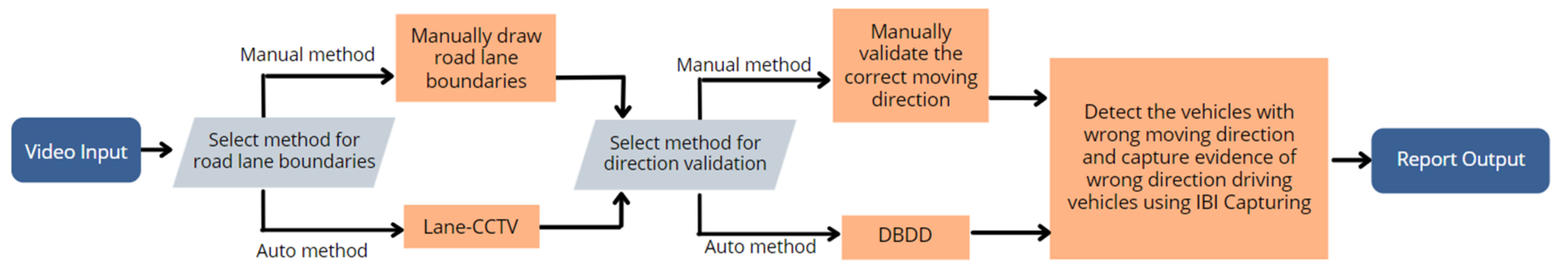
1.6. WrongWay-LVDC Framework

With the ideas and proposes for the three objectives, we propose the three systems that are functioned for each specific task, and each of them will be executed as an autonomous pipeline after the previous task is successfully performed. The output from the previous step will be received as the input for the next step. Therefore, we linked the three systems as subsequence tasks under an autonomous framework called WrongWay-LVDC, which stands for Lane detection, direction Validation, Detection of vehicles, and Capture the images. The three systems that are composed of this framework and are our contribution to this research are as follow:
  • Improved road lane boundary detection from CCTV (improved RLB-CCTV)
  • Direction validation and wrong-way driving vehicle detection using Distance-Based Direction Detection (DBDD)
  • Inside Boundary Image Capturing (IBI capturing)
The framework flow for WrongWay-LVDC is shown in Figure 2 below.
Figure 2 shows the framework of our proposed system. The system will detect the road boundaries using the improved RLB-CCTV algorithm. Then, the wrong-way driving validation and detection system will validate the correct moving direction of the vehicle on each detected road boundary using the DBDD algorithm. After the validation, the system will generate the reference value that will be used to measure the correct driving direction in each lane, and the detection part will be performed. As the system detects and tracks each vehicle in each lane in the detection part, it will compare the moving direction of the vehicle and whether it corresponds to the correct moving direction of each lane. The accumulating counters will count the number of correct and wrong driving vehicles. After the detection part ends, the counters will be summarized and shown to the user as a report so the user can evaluate the traffic of wrong-way driving level. If the intensity of wrong-way driving is high compared to correct-way driving, that area will be marked as a dangerous area, and the system will send an alert along with the vehicle counter-report as an output of the system to the users.
The three proposed sub-systems in the WrongWay-LVDC framework were developed as a prototype software application using Python [25] programming language. This developed framework can be tested using command lines in the Linux operating system [26]. The execution pipeline of this framework is shown in Figure 2. It is a one-time execution system, meaning that once we execute the framework, all sub-systems will be executed after one another, as shown in the pipeline. More information about the framework execution steps and versions are explained in detail in Section 2.5. The main idea, input, parameter, algorithms, and experimental results of our work are explained in the following sections of this paper. The first sub-system using the proposed improved RLB-CCTV algorithm is explained in Section 2.2. The second sub-system, the DBDD algorithm, is explained in Section 2.3. Lastly, the third sub-system, the IBI capturing feature algorithm, is explained in Section 2.4.

2. Materials and Methods
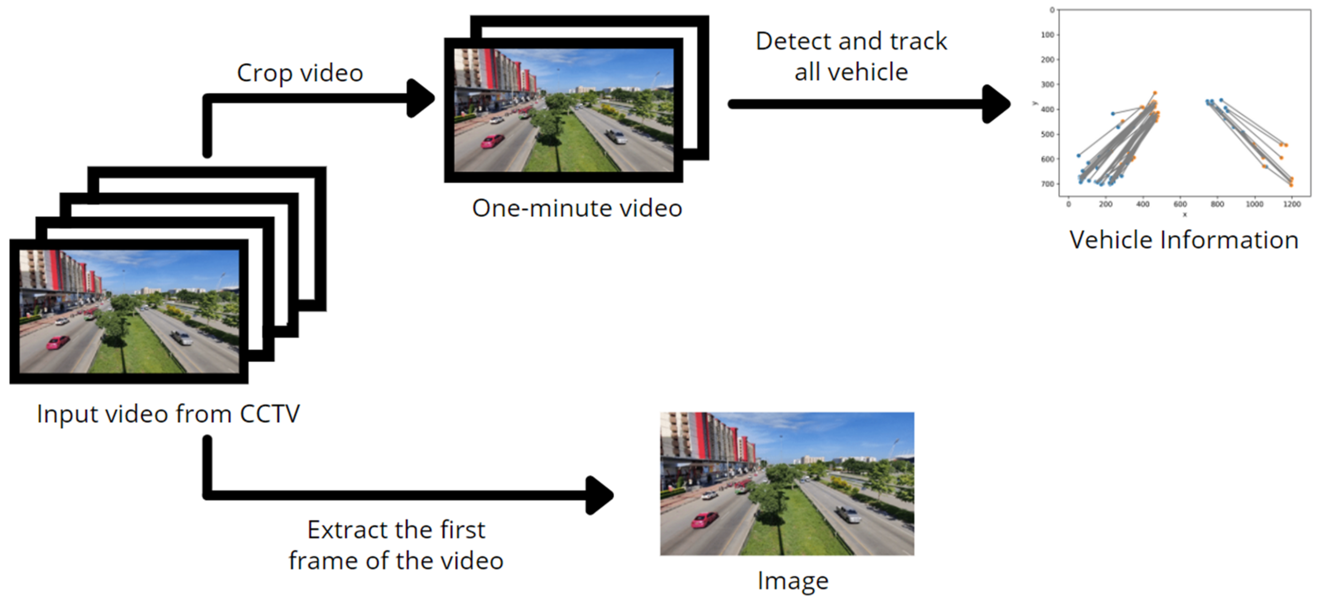
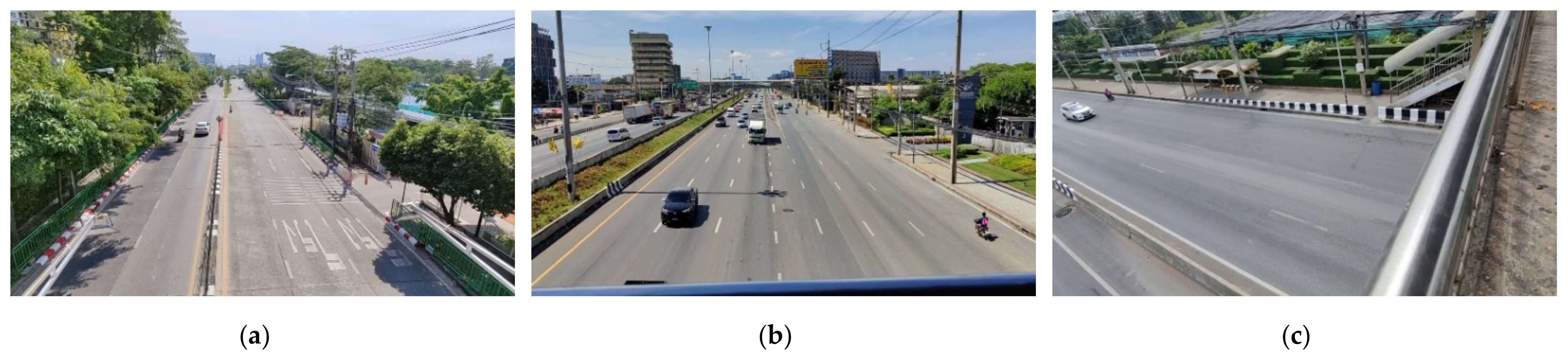
2.1. Input

The concept of our framework is to receive video inputs from CCTV. Typically, the CCTV will record video for 24 h a day and record the video periodically with a length of about one hour per video clip.
After we gather some video data of the road traffic in Thailand, we can observe several challenging factors to create our road lane detection algorithm. For example, some road is under construction, the road line color is pale, and the angle of the CCTVs are different. With the various condition of the road lane we have observed, the road with the unusual conditions might be our system’s limitation where our system might not be able to detect the lane line on those roads properly. Figure 3 shows the images of road lanes that do not have a clear lane line. Therefore, in this study, we set the research scope to select the following road conditions for our experiments.
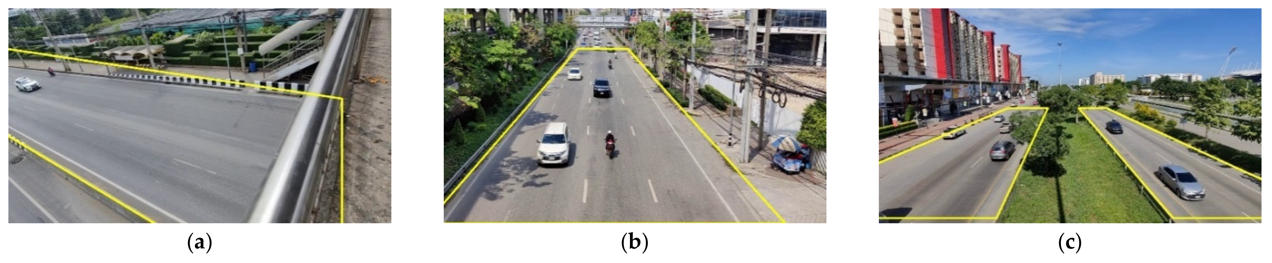
  • The road must be a straight line
  • The road must have a clear side road line or a clear footpath line
  • There should not be any objects blocking the side of the road
  • The road must not be under construction
  • The road should not have disturbing shadows from the side road objects.
Figure 3. Roads that do not pass the condition (a) The construction is on the left side of the road; (b) Many vehicles are blocking the side road.
Sustainability 14 10232 g003
The input videos will be further analyzed, processed, and transformed into two other forms of inputs: An image input and vehicle information. In Figure 4, we show the system flow of how our system can generate more data originating from a CCTV video.

2.1.1. Image Input

A captured image input is used in the road lane boundary detection algorithm for the image processing method to detect the road lane. This image input is derived from extracting the first frame of the input video using the OpenCV library [27] in the Python programming language.

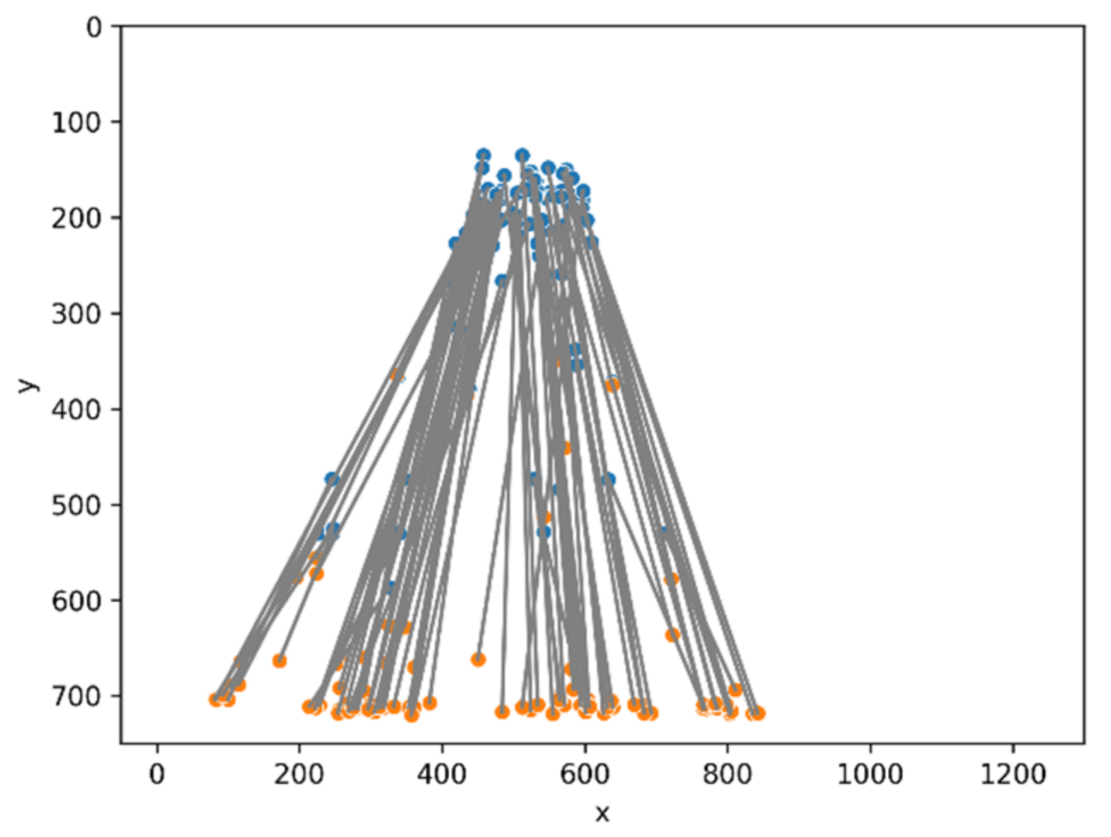
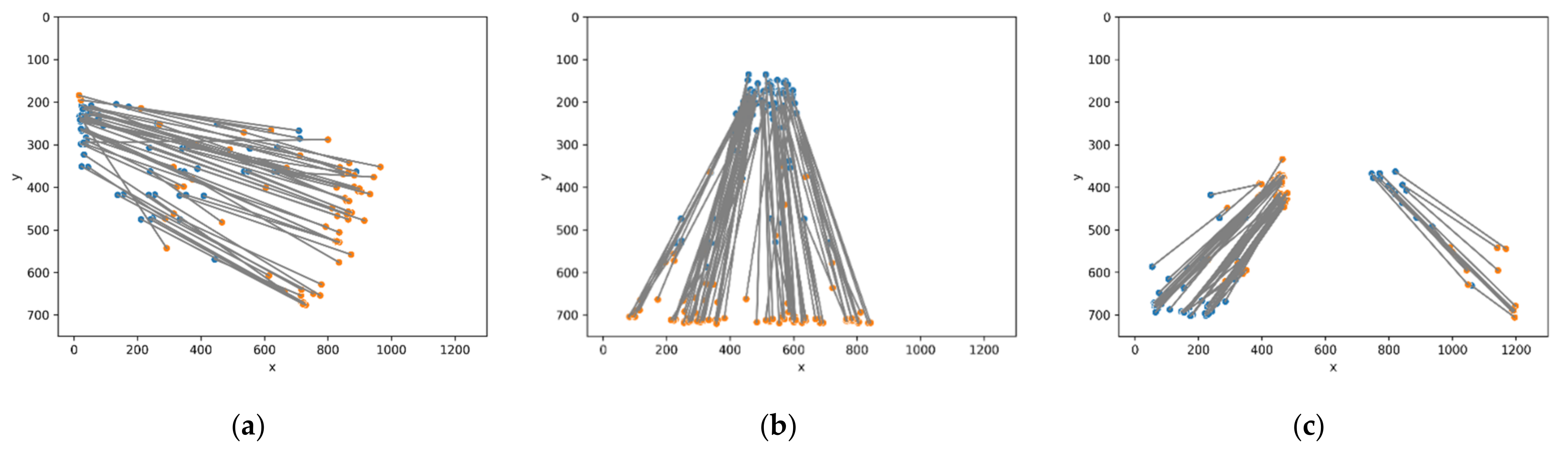
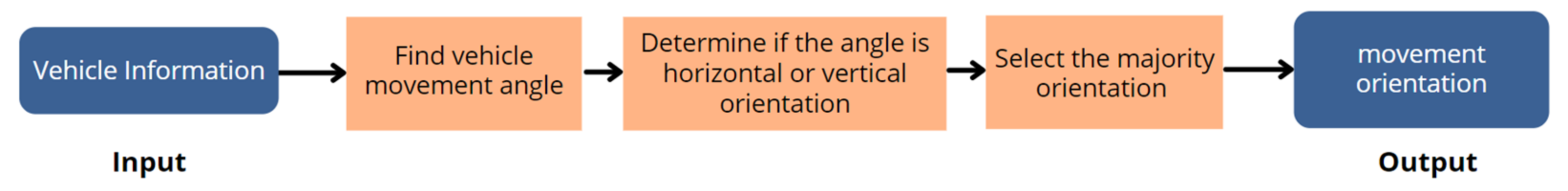
2.1.2. Vehicle Information

Vehicle information is a record of each vehicle’s start and stop locations within a video frame. There are three steps to obtain this input. First, crop the first one minute out of the main input video. Second, detect and track all vehicles moving inside the video frame regardless of the road lane. In this work, we use YOLOv4-Tiny for the object detection algorithm. YOLOv4-Tiny is an enhanced version of YOLOv4 [28]. It is smaller and suitable for running on small embedded systems. For the tracking algorithm, we chose the FastMOT algorithm [29]. FastMOT is improved from the Deep SORT tracking algorithm, where it is revised to be more suitable to run on small devices without bottleneck issues. The technique of FastMOT is to run the detector and feature extraction every N frame and use KLT to fill the gap efficiently. After all the vehicle has been tracked, the output will look like the image shown in Figure 5, where the plot is the summary of all movement vehicles within the time length of one minute. The orange dots inside the plot graph represent the location where each vehicle ID first appears inside the video frame or the start points. The blue dots represent the last location of the vehicle ID that has been tracked before the vehicle left the video frame or the stop points. The black lines link between the orange and blue dots, which represent the movement direction of each vehicle. Figure 5 shows that there is one road lane appearing in this video frame, where most of the vehicle in the lane is driving downward.

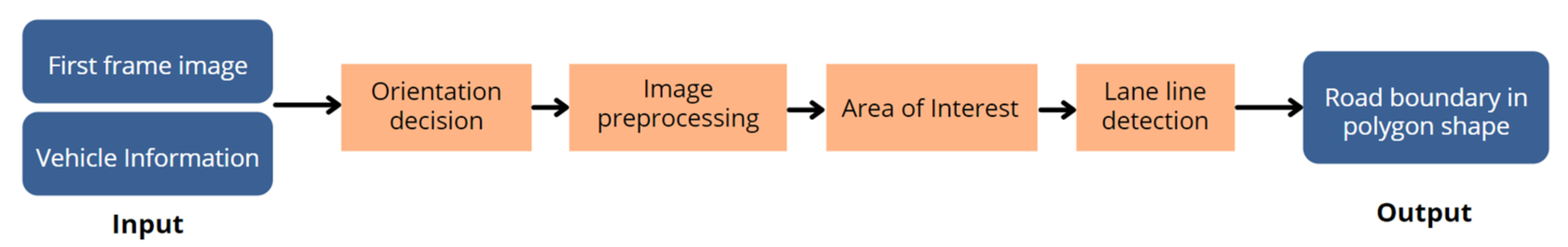
2.2. Improved Road Lane Boundaries Based on CCTV

The first sub-system executed in the WrongWay-LVDC is the improved RLB-CCTV algorithm. This algorithm is used to automatically detect the road lane boundary based on the image processing technique. Some previous work tried to perform lane detection based on image processing methods [19,20,21,22,23,24]. Most of that research has similar main steps to achieve the result; pre-processing of images, selecting areas of interest, and making lane line decisions. Nevertheless, there are many interesting techniques we can adopt and redesign to suit our research purpose. For example, the technique of Canny edge detection [30] in the image pre-processing step was used in [19,22,24]. This technique produces an output that focuses only on the contrast edge of the object inside the image, making the road lane clear, outstanding, and easy to detect. Another interesting technique is Hough transform [31]. All of the research papers [19,20,21,22,23,24] use Hough transform to make a decision and draw the line of the road lane. Another technique is Gaussian Blur [32], which is used in the image pre-processing step to reduce the image’s excessive noise [19,22,24].
According to the reviewed research, their approaches were designed for ADAS. Our research has a different purpose as we design for the CCTV camera angle. The setting of the CCTV camera mostly has a high and center position to view the road at a clear angle. With this position, the CCTV will see the road aligned vertically, as shown in Figure 6a,b. Moreover, we also consider another case where the CCTV is installed on the side of the road, which will make the angle the CCTV see the road aligned horizontally, as shown in Figure 6c.
These two cases of the camera angle have an impact on creating the lane detection algorithm. In our previous work, we created the road lane boundary detection for CCTV algorithm (RLB-CCTV) [33], which can only support and detect the vertical road lane in the video. However, if the road lane lies in the horizontal orientation, the algorithm will not be able to detect the road lane. With this limitation from our previous work, we have improved our algorithm to detect the road lane with both orientations. This improved algorithm will be called improved RLB-CCTV.
The improved RLB-CCTV consists of four main parts: orientation decision, image pre-processing, identifying areas of interest, and lane line decision. The inputs of this algorithm are image input and vehicle information. The system flow of the overall algorithm is shown in Figure 7.

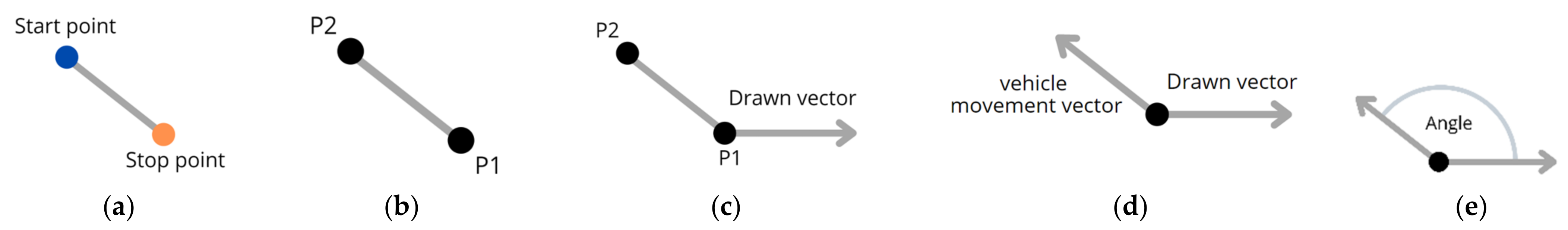
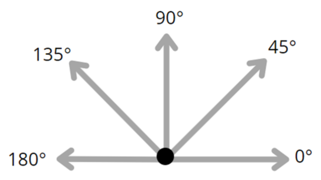
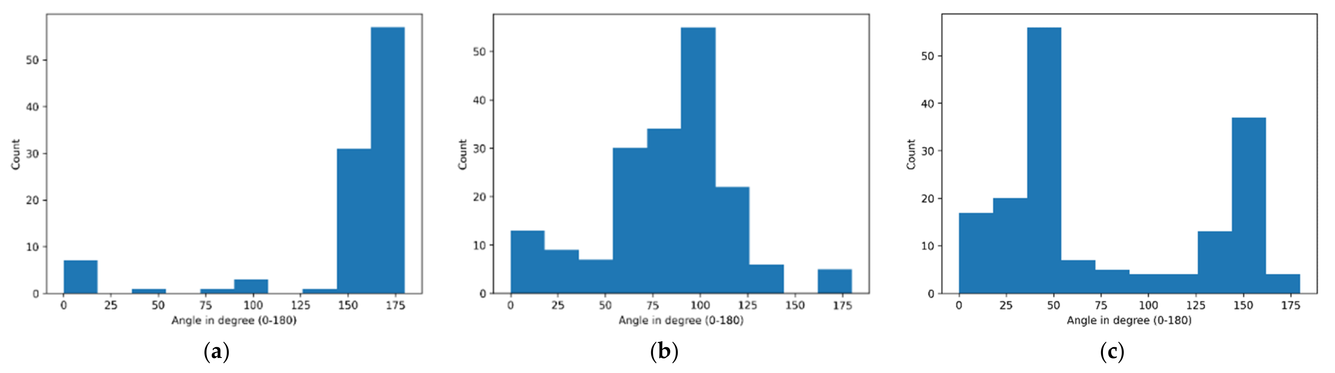
2.2.1. Orientation Decision

The first step in the improved RLB-CCTV algorithm is to determine the angular orientation of the input video, to detect whether the lane is aligned horizontal or vertical. The pseudocode of this step is represented in Algorithm 1. The input of this step is the vehicle information, as shown in the examples in Figure 8a–c.
As we can see in Figure 8, (a) contains a road lane with a horizontal angle, (b) contains a vertical angle, and (c) contains the vertical angle with two road lanes. We developed a method to let the system identify the orientation automatically, and the flow of this method is shown in Figure 9.
Our main idea is to find most of the vehicle’s movement angle and set the road orientation of that input video accordingly. For each vehicle movement, the information will compose of the start and stop points, as shown in Figure 10a. To obtain the vehicle movement vector, the head of the vector must be either the start or stop point depending on which point has a lower x value on a plot graph, as the pseudocode explained in Algorithm 1 (lines no. 3 to 9). As shown in Figure 10a, the stop point is plotted lower than the start point. Therefore, the location of the stop point will be relabeled as P1, and the location of the start point will be relabeled as P2 in Figure 10b.
The imaginary horizontal vector is being drawn from P1 point in Figure 10c, and the segment P1 and P2 will be converted into a vector in Figure 10d as well. With these two vectors, the angle between them will be found in Figure 10e. All possible vectors and angles are roughly shown in Figure 11. In this case, we will use the degree system with the range of 0 degrees to 180 degrees as the direction of the vector that indicates the angle in degree.
After we obtain the angle for each vehicle movement in the vehicle information, we have to set the range of the angle where we will consider it as a horizontal or vertical orientation. We set the condition as shown in Algorithm 1 on lines 11 and 13.
Algorithm 1. Pseudo Code for the Orientation Decision Step
Input: Vehicle Information
Output: Road Orientation
Auxiliary Variables: Horizontal Count, Vertical Count
Initialization: Horizontal Count = 0, Vertical Count = 0
Begin Orientation Decision Algorithm
1for(Each Vehicle MovementVehicle Information) do
2    Start location, Stop location = extract information (Each Vehicle Movement)
3    if (Start location (y) < Stop location(y)) then
4        Point 1 = Start location
5        Point 2 = Stop location
6    else
7        Point 1 = Stop location
8        Point 2 = Start location
9    end if
10    Each Angle = Find Angle (Point 1, Point 2)
11    if (Each Angle ≤ 180) AND (Each Angle > 155) OR (Each Angle ≥ 0) AND (Each Angle < 35) then
12        Horizontal Count = Horizontal Count + 1
13    else if (Each Angle ≥ 35) OR (Each Angle ≤ 155) then
14        Vertical Count = Vertical Count + 1
15    end if
16 end for
17if Horizontal Orient > Vertical Orient then
18    Road Orientation = Horizontal
19else
20    Road Orientation = Vertical
21end if
22return Road Orientation
End Orientation Decision Algorithm
After finding the angle of all vehicle information, the result is shown in the histogram plot, where Figure 12a is the histogram result of Figure 8a, Figure 12b is the result of Figure 8b, and Figure 12c is the result of Figure 8c. The angle result corresponds to the method we set, the range between 0 and 180, as well as the result of finding the road orientation, where Figure 12a is a vertical orientation, and Figure 12b is a horizontal orientation. However, Figure 12c is quite hard to identify with eyes which orientation is it, but as we compute it with our algorithm, it is a vertical orientation.

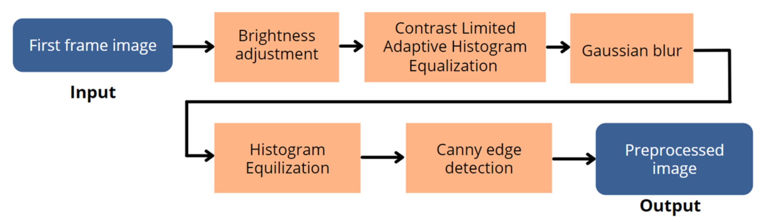
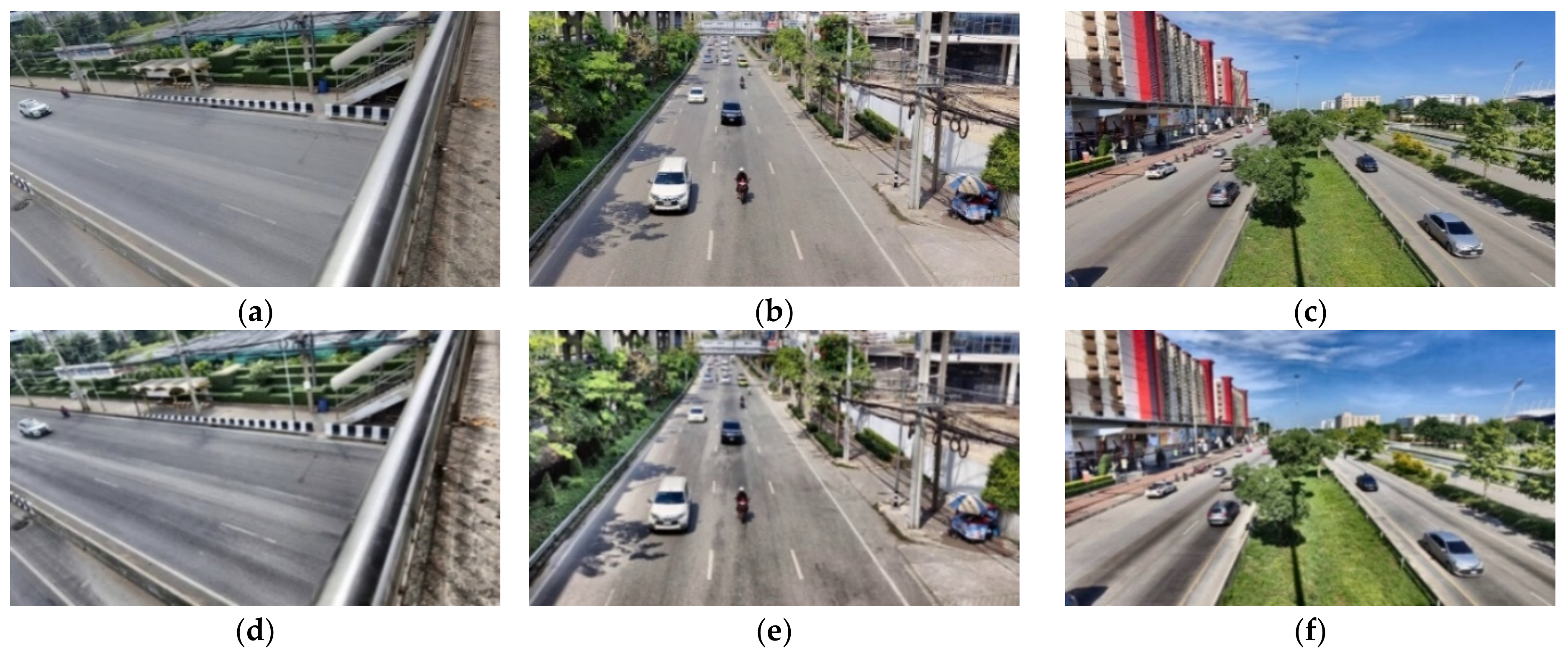
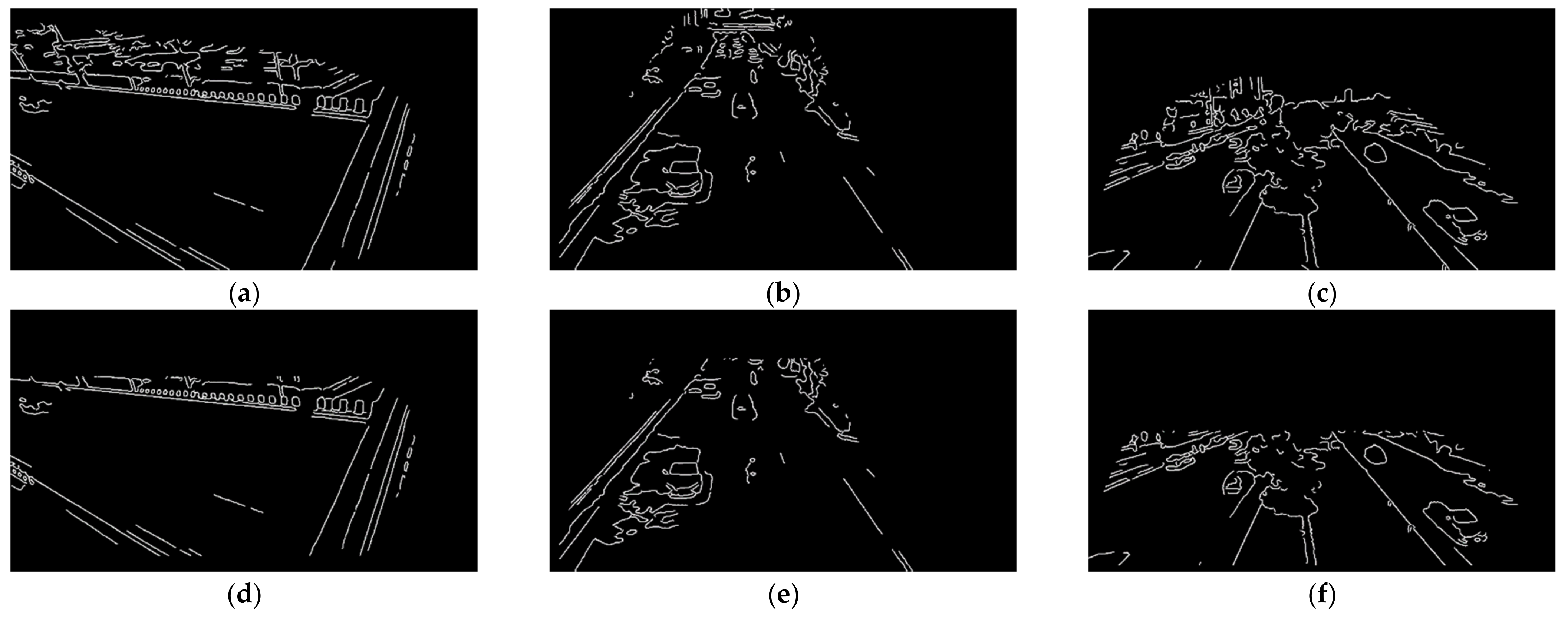
2.2.2. Image Preprocessing

In this step, the system performs the image pre-processing of the input image to extract only significant details such as the road lanes and remove the noises inside the image. The input image is pre-processed using five techniques, as shown in Figure 13. The detail of each technique is described as follows.
The first step is brightness adjustment. The system checks the brightness level of the input image by converting the image into grayscale and obtains the average pixel brightness value using the ImageStat [34] library module in Python. If the input image has a low brightness level, the output value will be near zero. If the image has a high brightness level, the output value will be near 255. To increase the image’s brightness, it will show some hidden detail that was dimmed and dark. However, the brightness should be increased according to the original image condition.
Increasing the image’s brightness will show some hidden detail that was dimmed and dark. However, the brightness should be increased according to the original image condition. If the brightness in the image is already high, we should not increase the brightness on that image anymore because that will cause brightness exposure. Therefore, the brightness value will be subtracted by the threshold value that we have set at 130. We tested several images to ensure that 130 is the adequate brightness level so the image will not be too bright or too dim. After we find the difference between the brightness value and the threshold value, we will use that difference value to increase the brightness of the original image by converting the image into the HSV system [35] and increasing the brightness according to the difference value we found. The result of brightness adjusting is shown in Figure 14a–c.
The second step is to increase the global contrast of the image by using Contrast Limited Adaptive Histogram Equalization (CLAHE) [36] to make the road line look clearer. In the third step, we use Gaussian Blur to exclude some unnecessary small details not to be drawn in the edge decision step. With the OpenCV library, we have to apply Gaussian Blur 6 times to make the road image cover and hide all small detail. The result of steps two and three are shown in Figure 14d–f.
The fourth step is to add Histogram Equalization [37] in OpenCV. The image needs to be converted into grayscale before applying this technique. The results are shown in Figure 15a–c, respectively. The image’s contrast is increased so that we can see more details in the image.
The fifth step is applying the Canny edge detection [27] to reduce the noise and focus on the object’s edge. The final output from the image pre-processing step is shown in Figure 15d–f.

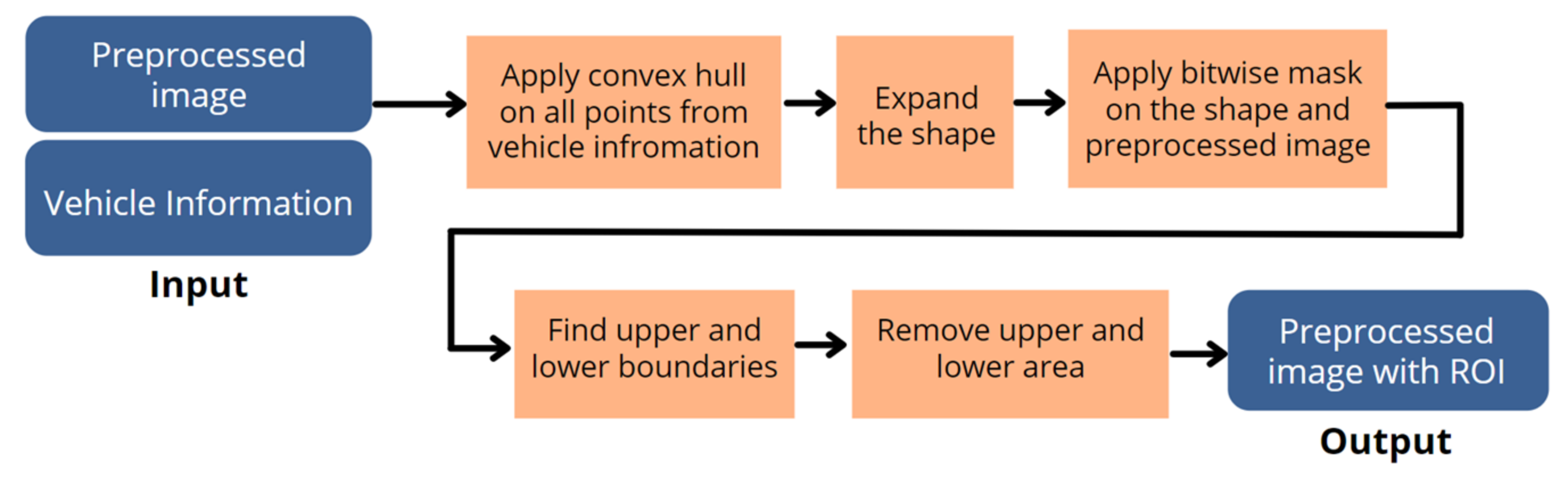
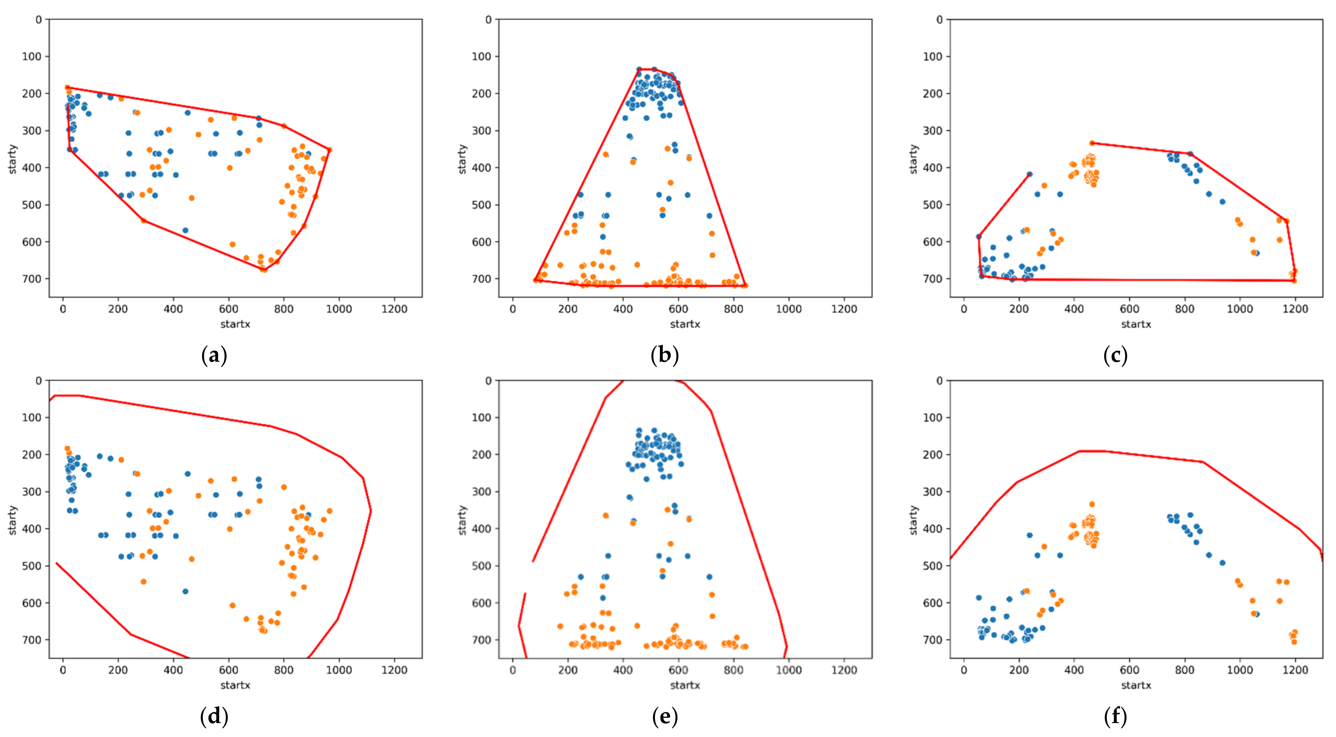
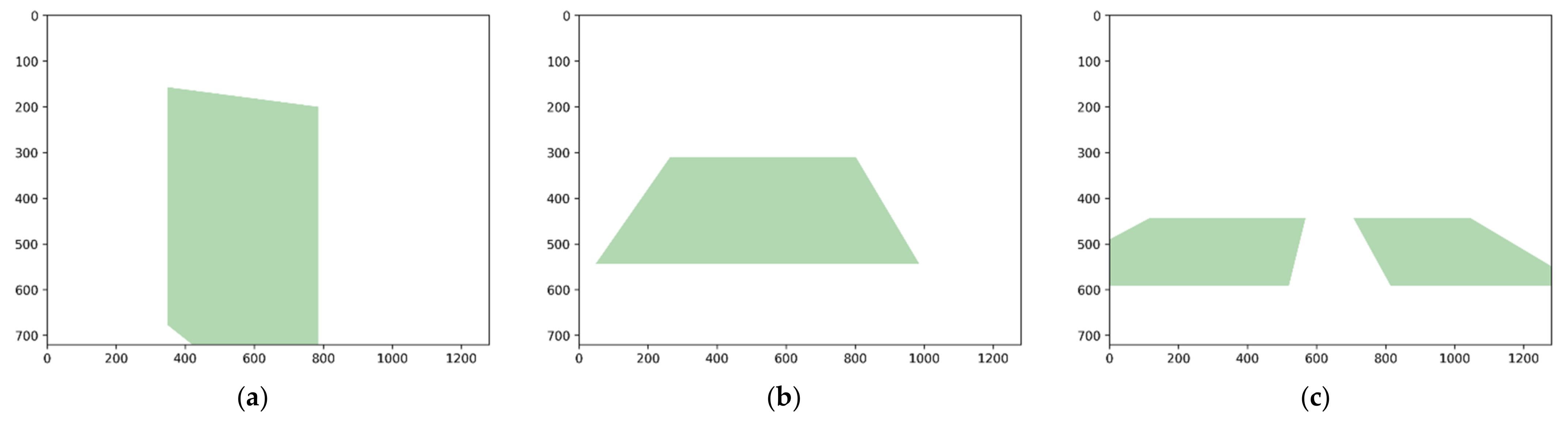
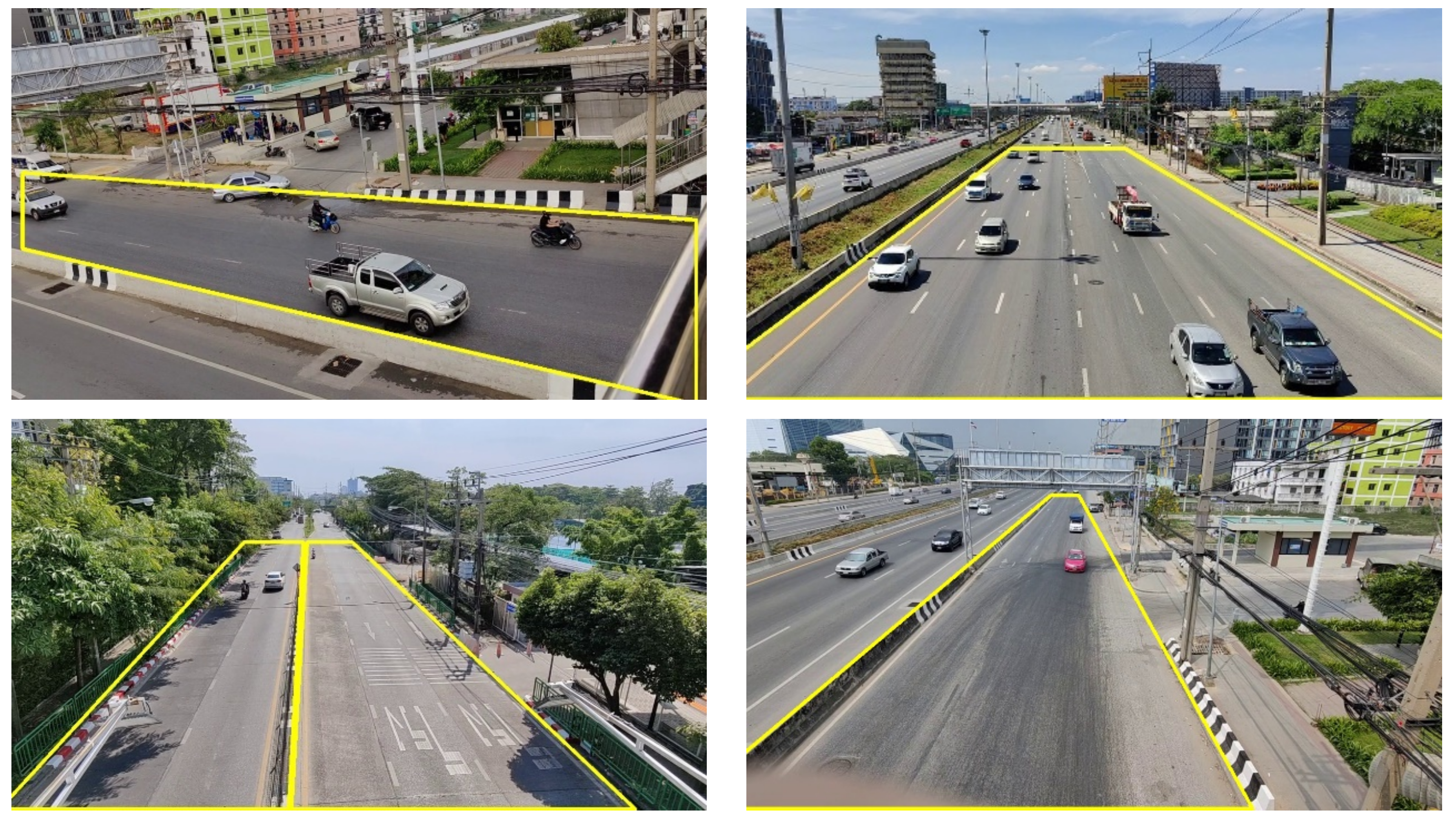
2.2.3. Area of Interest

After we have the pre-processed image, we can see that the image still includes some side road areas where it will not contribute to our algorithm’s purpose. These unwanted areas will decrease the lane line detection accuracy. The simplest method is to identify the Area of Interest (AOI). However, each road image has a unique position of AOI, so we should not fix the AOI for all images. The system flow for this step is shown in Figure 16.
The vehicle information allows the system to know the location where the vehicles are likely to drive. The vehicle drives on roads; therefore, the roads are our target AOI. Based on the assumption, we focus on the area where vehicles are driving inside the video frame, and that area will be used as the AOI. We use the technique of the convex hull [38], which draws the lines that connect the dots that are positioned in the outer area of the geometric shape. We apply the convex hull onto the vehicle information and draw a shape that wraps around all points (start point and stop points of the vehicles) as shown in Figure 17a–c. The red line shape is considered as the area where the vehicles appear.
However, those areas do not include the road sideline as the vehicle will not drive on the side road. Then, we need to increment the convex hull shape we drew to be larger by applying the Buffer points method and drawing a convex hull on the new buffer points. As a result, the areas are expanded and cover the road line, as shown in Figure 17d–f, where we will use this area as the AOI. Since we have the AOI area, the next step is to overlay the AOI area onto the output image from the image pre-processing part by using the technique of OpenCV called bitwise mask [39]. The bitwise mask will select to keep the part of the image we want and discard the rest. The result of this step is shown in Figure 18a–c, where we can see that these two images have a different location and size of the AOI, and the drawn AOI fit to show the road area only for that image. At this stage, we can see that Figure 18a has some sideroad noises on the top, similar to Figure 18b, where the top part of the image still has some noise. To remove those noises, we use the upper and lower boundary techniques mentioned in [22]. We use the same technique to remove the sky area of the image. To find the upper and lower boundary, we use the vehicle information that contains the points (start or stop points) with the highest and lowest y value in the cartesian coordinate system. These points are used to draw horizontal lines, which refer to as upper and lower boundaries. We also apply the bitwise mask of the upper and lower boundaries onto the image. The final result is shown in Figure 18d–f. The noise is removed, and the image is ready to be used in the lane line decision step using the RLB-CCTV algorithm.

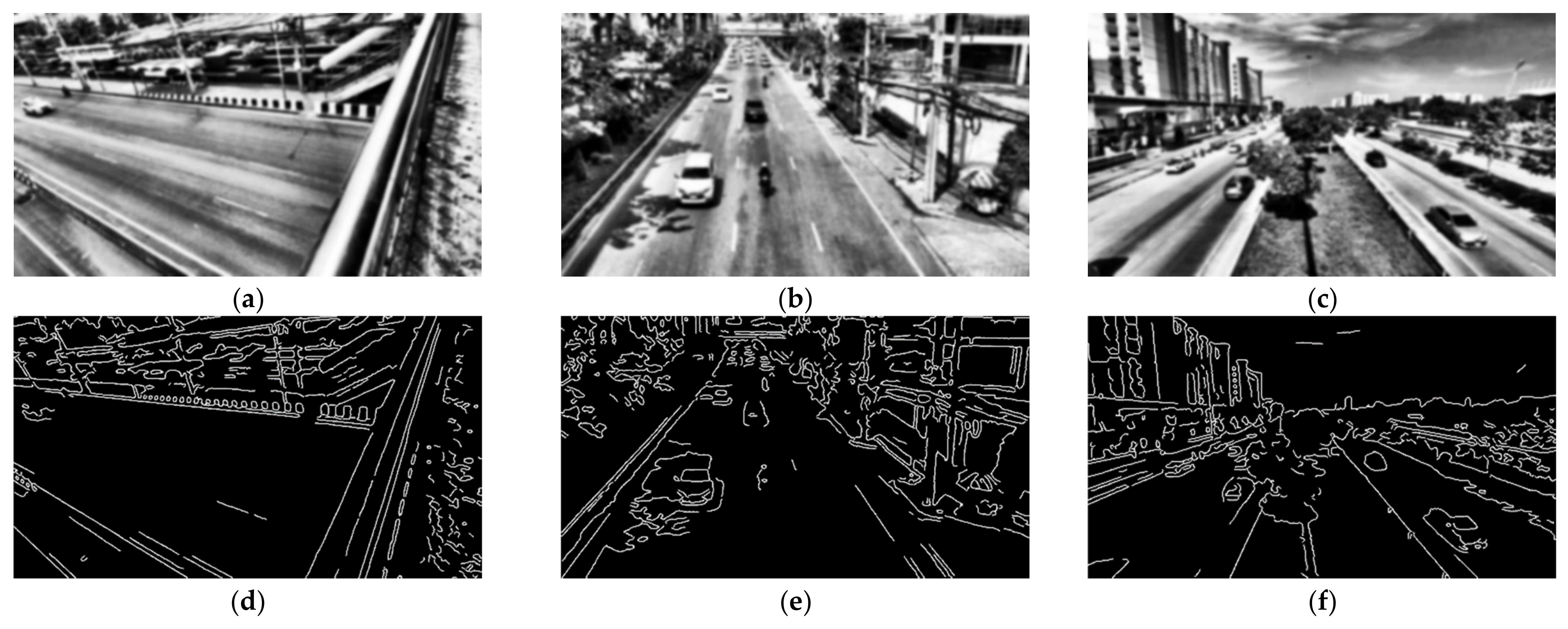
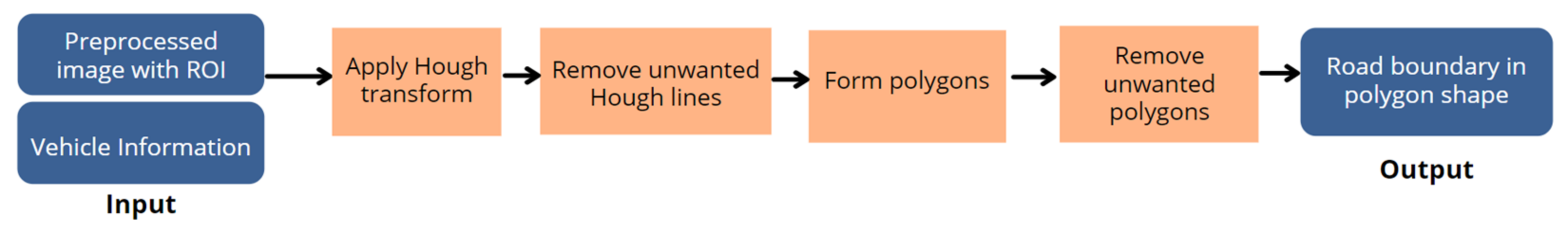
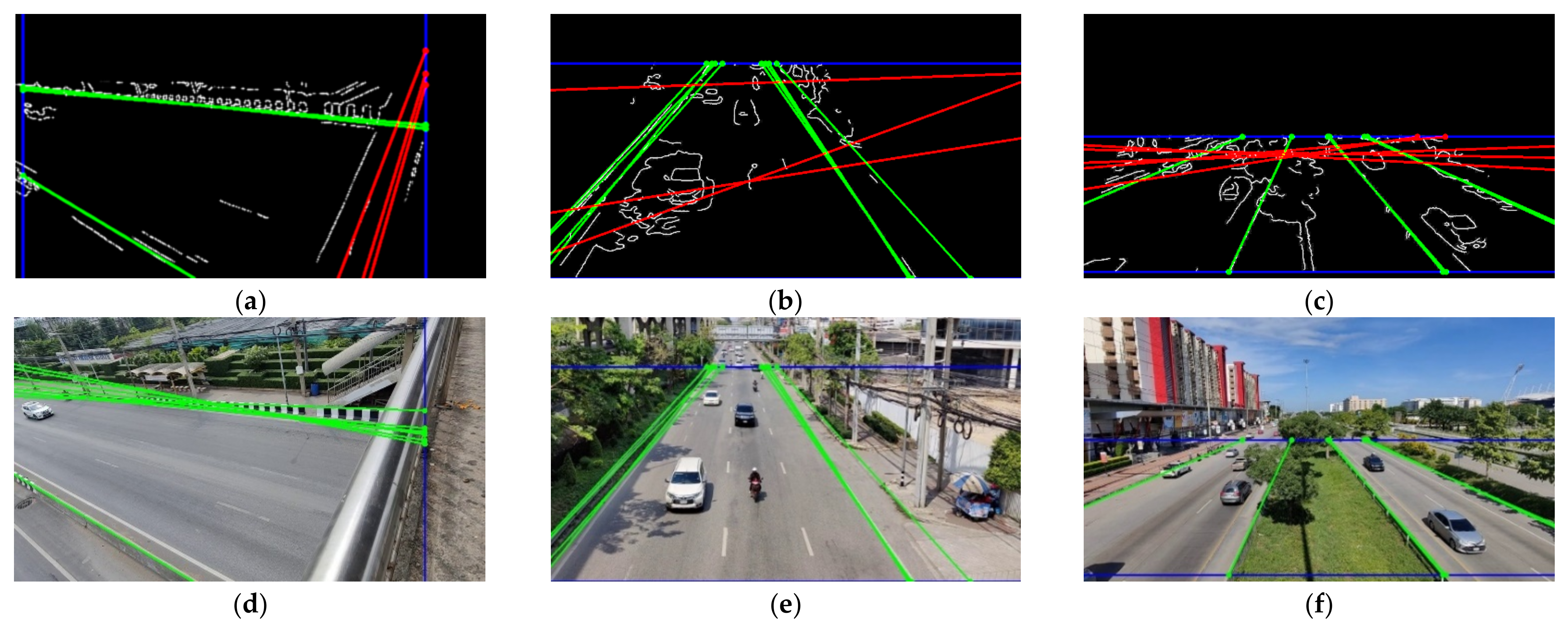
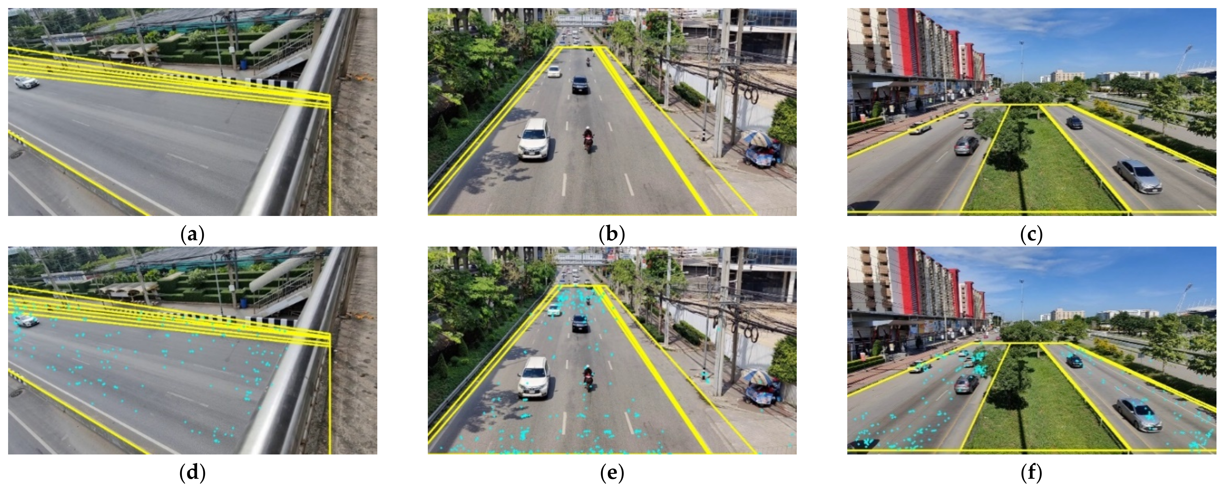
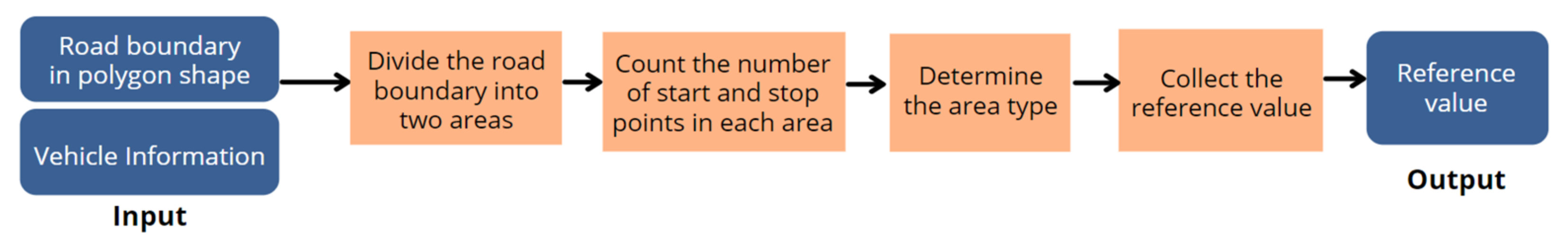
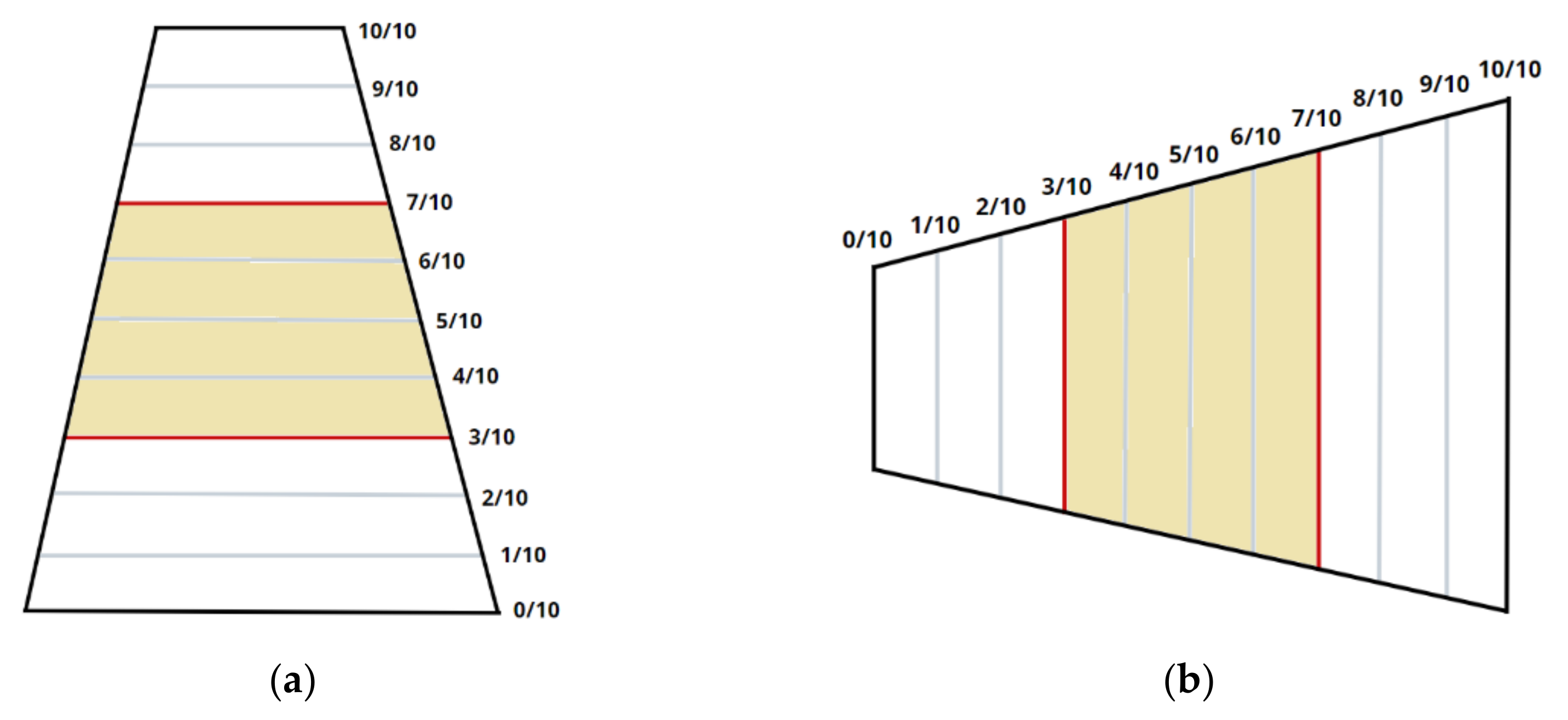
2.2.4. Boundary Detection

In lane line detection, the algorithm we use to detect the line is the Hough transform algorithm [28]. There is a decision to select the most accurate Hough line; the step of making this decision is shown in Figure 19. We set the system to draw 12 Hough lines in one image to ensure all expected lane lines will be drawn. However, some unwanted Hough line has been drawn along the way, as shown in Figure 20a–c. The red Hough line is the line where we detect it as an incorrect drawing. We filter those lines based on the lane’s orientation, which we obtained from the orientation decision. The system will check the slope value of each line, where the slope is calculated from the two endpoints of the Hough line. If the orientation is vertical, as shown in Figure 20b or Figure 20c, the blue color upper and lower boundaries will be drawn, and the endpoints of the Hough lines will meet there. The slope of the accepted Hough line in the vertical orientation must meet this condition.
|(y value of endpoint 2 − y value of endpoint 1) × 2| > |x value of endpoint 2 − x value of endpoint 1|
If the orientation is horizontal, as shown in Figure 20a, the left and right boundaries will be drawn, and the endpoints of the Hough lines will be extended to meet the two blue boundary lines. The slope of the accepted Hough line must meet this condition.
|(x value of endpoint 2 − x value of endpoint 1) × 2| > |y value of endpoint 2 − y value of endpoint 1|
Figure 19. System flow of lane line detection step.
Sustainability 14 10232 g019
Figure 20. Apply Hough transform to draw straight lines on the image. The red lines are the unwanted Hough lines we received. The green lines are the correct Hough lines we expected (a) Horizontal orientation; (b) Vertical orientation; (c) Vertical orientation with two lanes. Remove the unwanted red Hough lines (d) Horizontal orientation; (e) Vertical orientation; (f) Vertical orientation with two lanes.
Sustainability 14 10232 g020
The red Hough line in Figure 20a–c is an example to show the lines that do not meet the above condition we stated. As an output, the accepted Hough lines are drawn on the original input image to compare and check the correctness (see Figure 20d–f). We can see that several accepted lines are drawn on the image. We must remove the duplicated lines; however, which lines should be removed? If we remove the inner lines and keep only the most-outer lines, that would work only in the case shown in Figure 20d,e, but would not work in the case where there is two-way traffic, as shown in Figure 20f.
In order to design a method that can cover several cases, the next step is to draw the polygon area from the accepted Hough line. To clearly explain the procedures and the main idea of the polygon forming method for the car that moves in a vertical orientation, we can describe it using the pseudocode as shown in Algorithm 2. Please note that this code shows only one step of many steps used in the improved RLB-CCTV algorithm. First, we gather the locations of all intersection points between Hough lines and boundary lines. If the orientation is vertical, we will gather the x value of all intersection points, and if the orientation is horizontal, we will gather the y value of all intersection points. In the case of vertical, we represent a list of x values of the intersection points in the upper boundary using UpperX, where upperxi represents each x value contained in UpperX.
UpperX = [upperx1, upperx2, upperx3, upperx4, …, upperxn]
LowerX represents a list of the x values of the intersection points in the upper boundary, where lowerxi represents each x value contained in LowerX:
LowerX = [lowerx1, lowerx2, lowerx3, lowerx4, …, lowerxn]
Both UpperX and LowerX are sorted ascendingly. In the vertical orientation, the y value of the lower and upper boundaries will be fixed, as the boundary is a horizontal line. Therefore, the y value is a constant for all intersections of the lower and upper boundaries. In this case, we assign the y value of the upper boundary as UpperY and the y value of the lower boundary as LY. To create a four-corner polygon, we select the four points from the two lists, every two values from each list as the pseudocode shown in Algorithm 2. Line 7 in Algorithm 2 represents the method of creating the polygon using Shapely geometry python library [40]. This method requires only four points as corners to draw a polygon.
Algorithm 2. Pseudo Code for Polygon Forming in Vertical Orientation
Input: UX, LX, UY, LY
Output: Polygon corners
Auxiliary Variables: Polygon_list
Initialization: Polygon_list = []
Begin Polygon Forming in Vertical Orientation
1While (element number in UX > 1) do
2   Current_intersect_1 = UX [0]
3   Current_intersect_2 = LX [0]
4   Next_intersect_1 = UX [1]
5   Next_intersect_2 = LX [1]
6   Polygon corners = [[Current_intersect_1, UY], [next_intersect_1, UY], [next_intersect_2, LY], [Current_intersect_2, LY]]
7   Polygon_list.append(Shapely.polygon(Polygon corners))
8   Remove UX [0] from UX
9   Remove LX [0] from LX
10 end while
11return Polygon_list
End Polygon Forming in Vertical Orientation
In the case of horizontal orientation, the algorithm used to form the polygon for a horizontal camera angle is similar to the vertical one. We gather the intersection point between accepted Hough lines and the two left and right vertical boundaries, as shown in an example in Figure 20d. We gather the x value of all intersection points. LeftY represents a list of the y values of the intersection point in the left boundary, and leftyi represents each y value contained in LeftY.
LeftY = [lefty1, lefty2, lefty3, lefty4, …, leftyn]
RightY represents a list of the y values of the intersection point in the right boundary and rightyi represents each y value contained in RightY.
RightY = [righty1, righty2, righty3, righty4, …, rightyn]
Similar to the vertical orientation, the intersection x value of the horizontal orientation case will be constant numbers, represented with LeftX and RightX. The algorithm to form the polygon for a horizontal orientation, which is a step among many steps inside the improved RLB-CCTV algorithm, is as shown in the pseudocode in Algorithm 3.
Algorithm 3. Pseudo Code for Polygon Forming in Horizontal Orientation
Input: LeftX, RightX, LeftY, RightY
Output: Polygon corners
Auxiliary Variables: Polygon_list
Initialization: Polygon_list = []
Begin Polygon Forming in Horizontal Orientation
1While (element number in LeftY > 1) do
2   Cur_intersect_1 = LeftY [0]
3   Cur_intersect_2 = RightY [0]
4   Next_intersect_1 = LeftY [1]
5   Next_intersect_2 = RightY [1]
6   Polygon corners = [[XLeft, Cur_intersect_1], [XLeft, next_intersect_1], [XRight, next_intersect_2], [XRight, Cur_intersect_2]]
7   Polygon_list.append(Shapely.polygon(Polygon corners))
8   Remove LeftY [0] from LeftY
9   Remove RightY [0] from RightY
10end while
11 return Polygon_list
End Polygon Forming in Horizontal Orientation
The images of the plotted polygons are shown in Figure 21a–c. We can see that some areas in the polygons are not road lanes. We must determine which polygon correctly covers road areas by performing another method that is overlaying the vehicle information (start and stop points) onto the image (see Figure 21d–f). It is obvious in Figure 21f that some area does not have any start or stop points, such as the grass area in the middle of the two roads. With this observation, we set the conditions for selecting good polygon areas. The number of points inside each polygon is set as the below equation.
Points = [num_point1, num_point2, num_point3, num_point4, …, num_pointn]
Since we know the number of points inside each polygon, next, we will check the number of points with the given condition. The polygons that have a number of points less than 20 will be removed. Based on our tests, 20 is an appropriate number for this condition.
A c c e p t e d   P o l y g o n s = A d d   t o   a c c e p t e d   p o l y g o n   l i s t , n u m   p o i n t   20 r e m o v e   t h e   p o l y g o n , n u m   p o i n t < 20
Figure 21. Form polygons; (a) Horizontal orientation; (b) Vertical orientation; (c) Vertical orientation with two lanes. Overlay start and stop point from vehicle information on the polygons; (d) Horizontal orientation; (e) Vertical orientation; (f) Vertical orientation with two lanes.
Sustainability 14 10232 g021
After checking all polygons, we should have polygons representing the road areas. Sometimes, an area of the road is separated into two areas due to the detection of Hough transform that detects the road’s centerline. To resolve this issue, we set a condition to merge two areas next to each other and correctly identify them as one area. The result of this step is shown in Figure 22a–c.

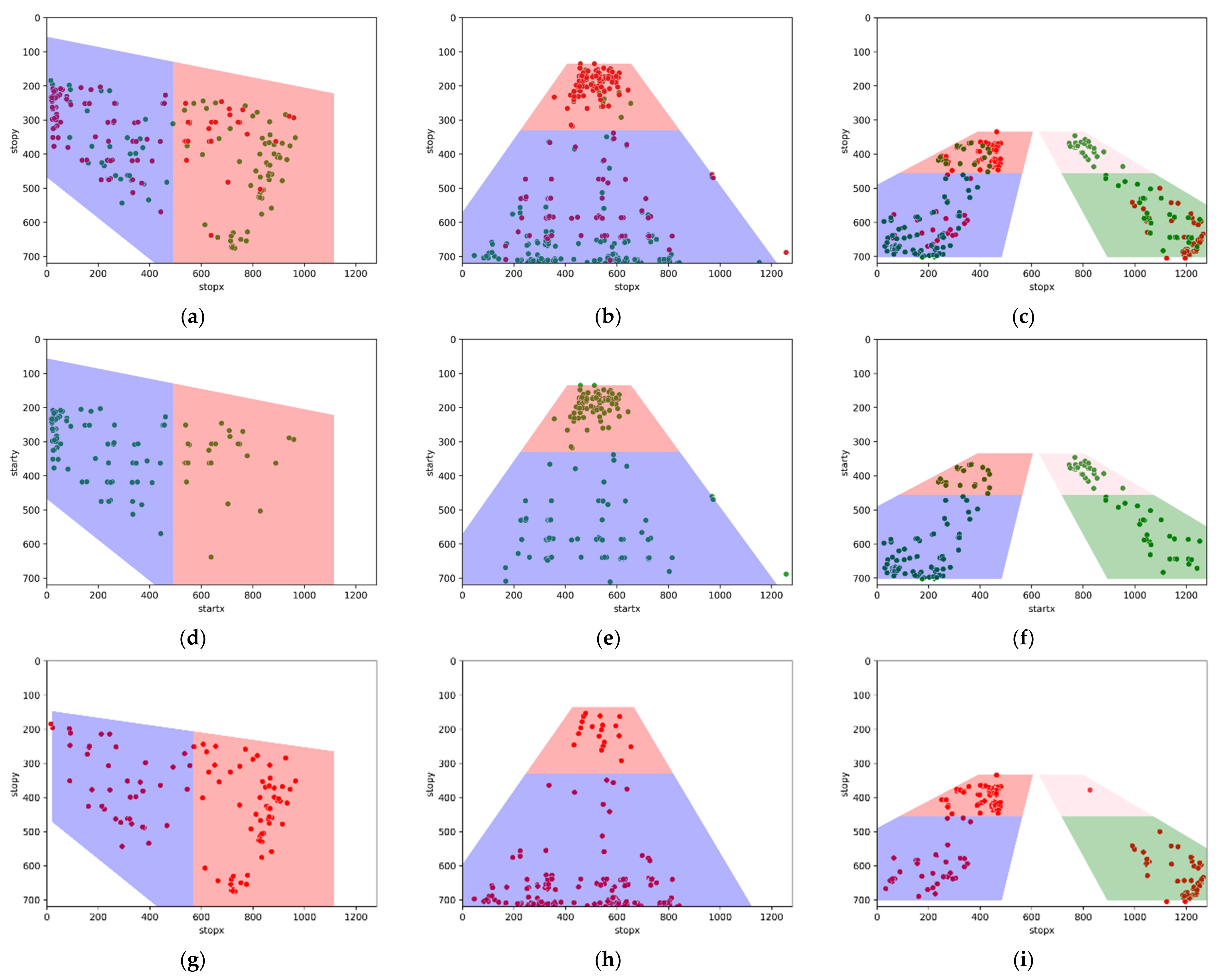
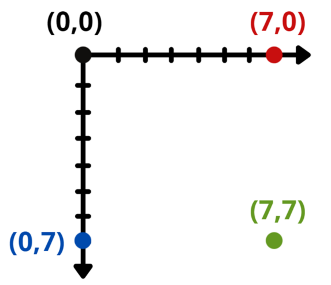
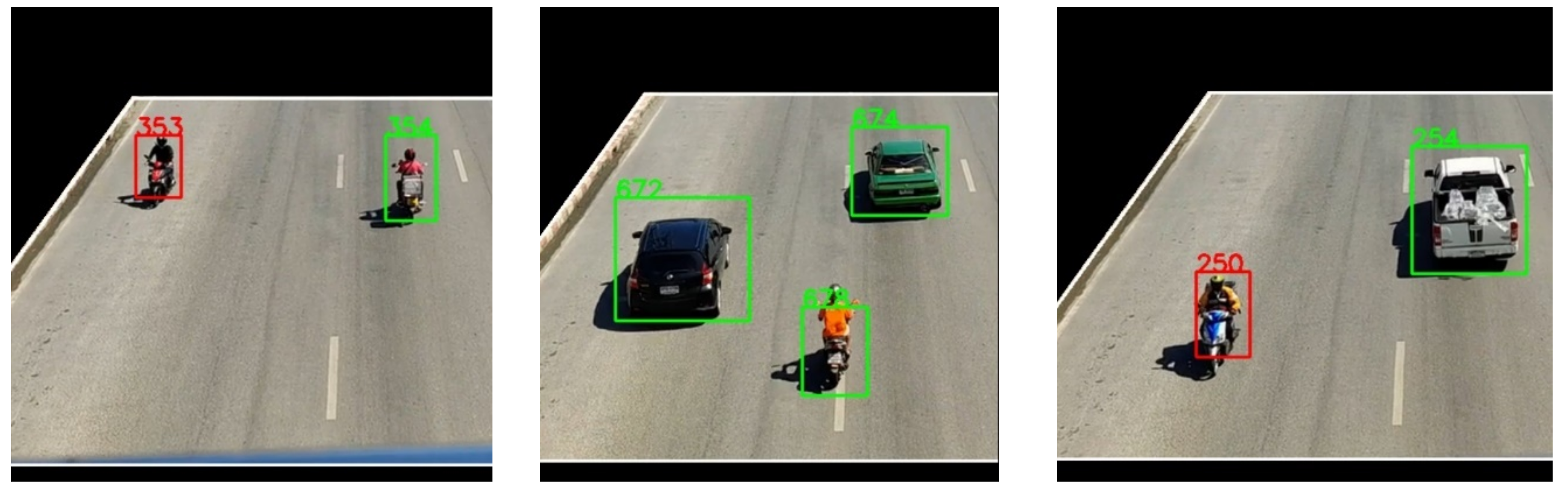
2.3. Distance-Based Direction Detection

The detected lane from the improved RLB-CCTV algorithm is used as an input for the Distance-Based Direction Detection algorithm (DBDD) algorithm. The DBDD algorithm is the second algorithm in the WrongWay-LVDC framework. This algorithm automatically detects the correct moving direction of each road lane. Many techniques have been introduced to verify and detect wrong-way driving vehicles [4,7,8]. In our previous research [41], we introduced the Majority Based Correct Direction Detection (MBCDD), an algorithm that can validate the correct direction for each road lane and detect the vehicle that drives in the wrong direction automatically. However, our previously proposed method still has some areas that need to be improved. MBCDD requires a one-minute cropped input video as input for validation, differently from DBDD, where it requires vehicle information. Even though the MBCDD is accurate and fast, in the process of direction validation on the edge device, it took twice as long compared to the length of the input video. With this flaw, we tried to improve the algorithm and eventually came up with a more optimal algorithm that is more suitable to run on an embedded system. This newly proposed algorithm is called the Distance-Based Direction Detection algorithm (DBDD). DBDD consists of two main parts: the validation and detection parts, where the overall system flow is shown in Figure 23.
In DBDD, the required input is the detected road lane boundary from the improved RLB-CCTV and the vehicle information. There are five steps to perform this validation in DBDD.
We divide the road lane area into two halves. If the orientation is vertical, the area will be divided into upper and lower areas. If the orientation is horizontal, the area will be divided into left and right. The second step is to overlay all the vehicle information onto the divided areas. As shown in Figure 24a–c, the red dots are the start location of each vehicle, and the green dots are the stop location of each vehicle. With this information, we can see vehicles’ start locations (red points), as shown in Figure 24b. Similarly, the stop location of vehicles tends to end in the lower area. To better visualize, Figure 24d–f were plotted to show only the start locations, and Figure 24g–i show only the stop locations of all vehicles. The third step is to make the decision.
We compare the number of dots in each area for each start and stop location. If the area has more start dots than the stop dots, then the area is the start area. If the area has more stop dots than the start dots, then the area is the stop area. We color the start area with green color and stop area with red color as shown in Figure 25a–c. The fourth step of the validation part is to plot the reference stopping point. Assuming that a vehicle is driving correctly in Figure 25b, the vehicle start location should start from the upper area and come down to the stop area. This is the general moving behavior the vehicle should be. In this step, we set a reference point on the stop area’s side. The reference point only stores the y value from the cartesian coordinate system, where the y value is obtained from the location of the further edge of the stop area. This reference point is used to check the distance between the vehicle’s location and the reference point. The last step is to calculate the distance and determine if a vehicle is driving in the correct direction or wrong direction. The distance will be constantly calculated frame by frame as the video is running. The distance between the start location of each vehicle and the reference point will be kept as an initial distance value. As the vehicle is moving, the second location of the vehicle will be updated. The system will calculate the new distance value as well.
In this stage, the system will compare the old and new distances. If the value decreases, it means that the vehicle is driving toward the reference point or the vehicle is driving in the correct direction. However, if the value increases, it means that the vehicle is driving away from the reference point or the vehicle is driving in the wrong direction. In the third frame of the video, the new distance value is calculated. The system will compare this distance value with the first initial distance value to confirm the moving direction of the vehicle.
With the concept of the reference point, we can observe the moving direction of each vehicle that drives inside the boundary. Moreover, we have considered the case where the lane boundary could be shorter in length for the shorter computing time of the system and a higher accuracy rate. The system is designed to track all vehicles inside the boundary and calculate the distance between each vehicle and the reference point. If the length of the road is long, the calculation on each vehicle is also longer. We used YOLOv4 Tiny to detect the vehicles on the road and focused on detecting the vehicle with visible size. There are some far vehicles that would cause confusion to the detector for the two stated reasons. We cropped the length of the road boundary by dividing the road into 10 ranges, as shown in Figure 26a,b.
In the range of 3/10 to 7/10 will be the focused section of the DBDD algorithm. We chose this range of sections based on the result when we tested the sample video on our proposed system. We remove the range 0/10 to 3/10 because as the vehicle approaches the camera in the vertical orientation, the discontinued tracking is likely to happen in this case. We removed the range 7/10 to 10/10 because the far objects are hardly detected. The remaining range is adequate for the system to detect each vehicle by the time they are moving, and objects are not too close nor too far. For the horizontal orientation (Figure 26b), we cropped the range to reduce computation time. As a result, the road boundaries from Figure 25 are cropped as shown in Figure 27.

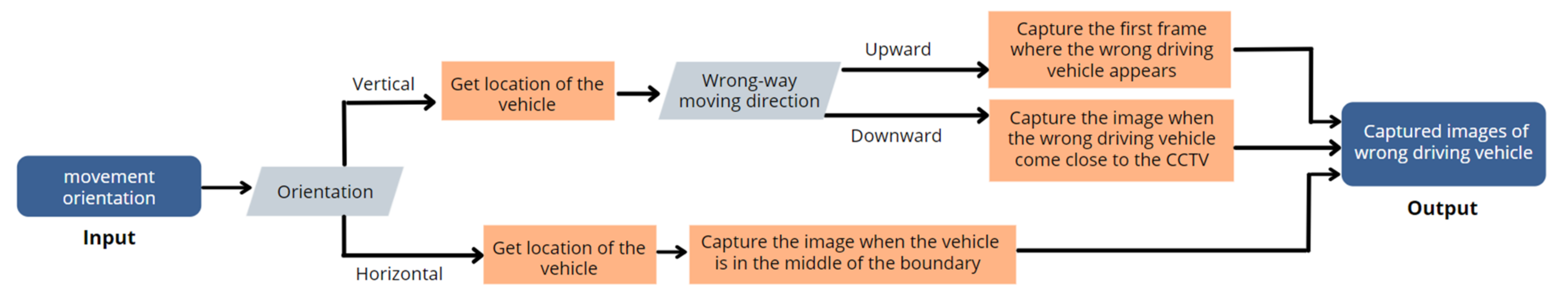
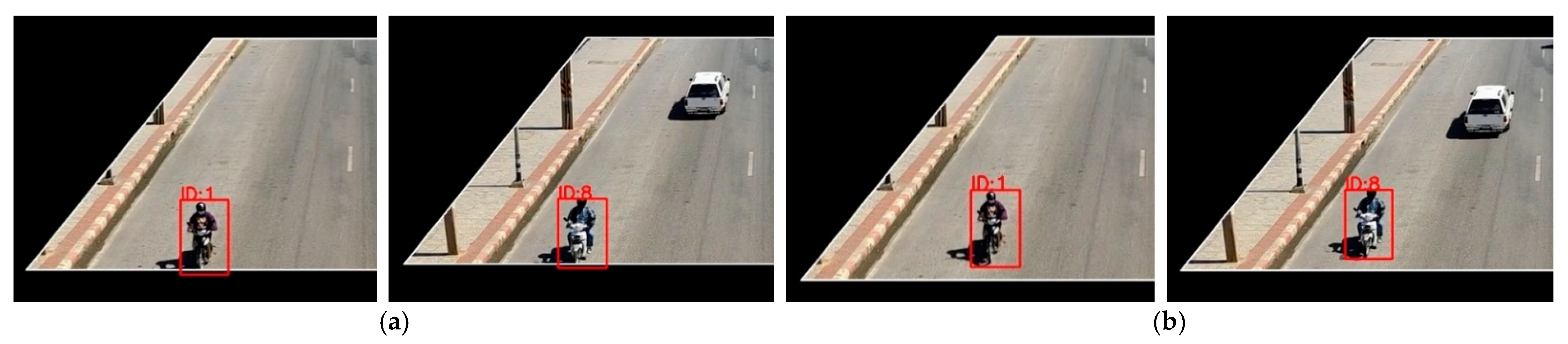
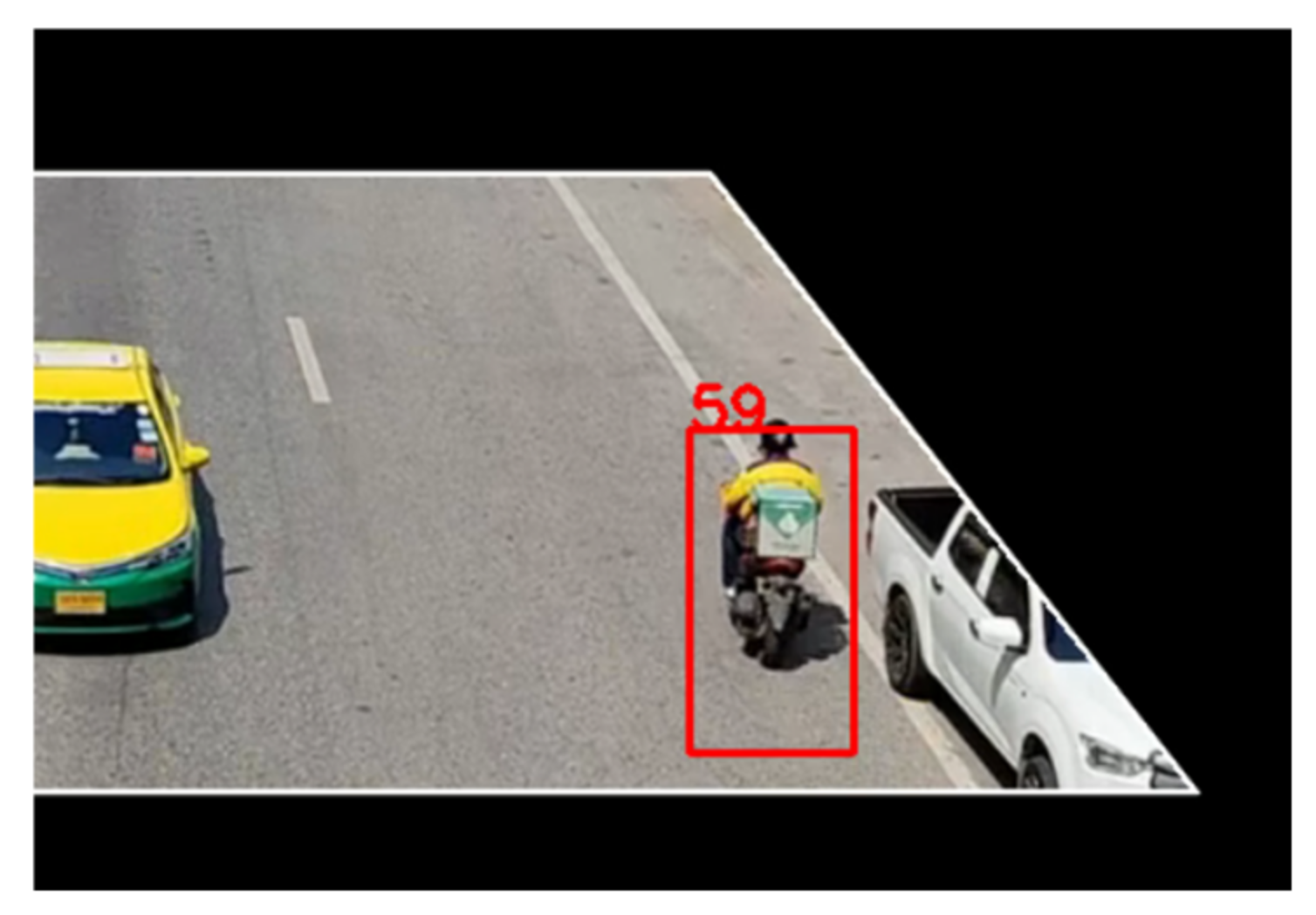
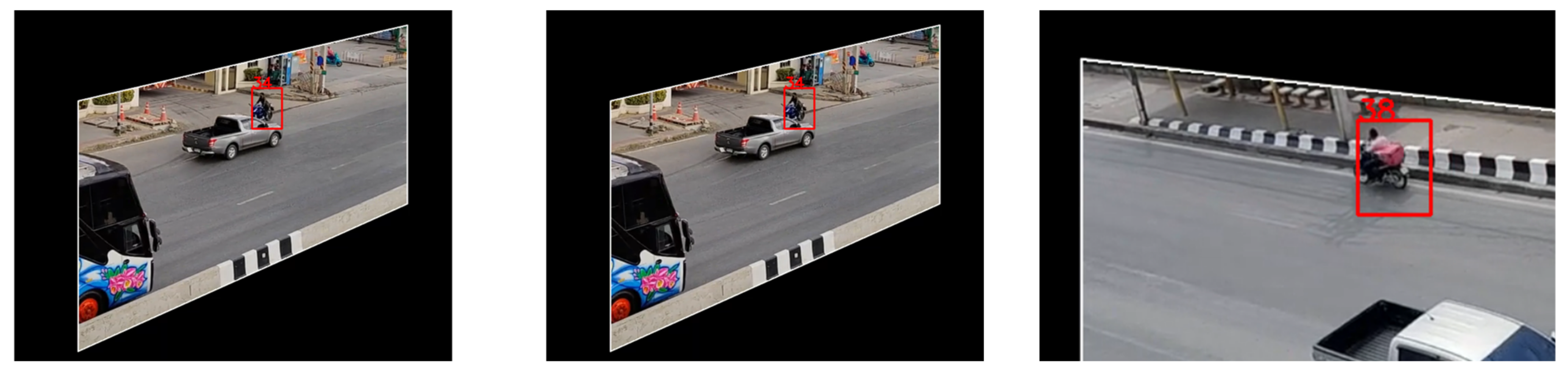
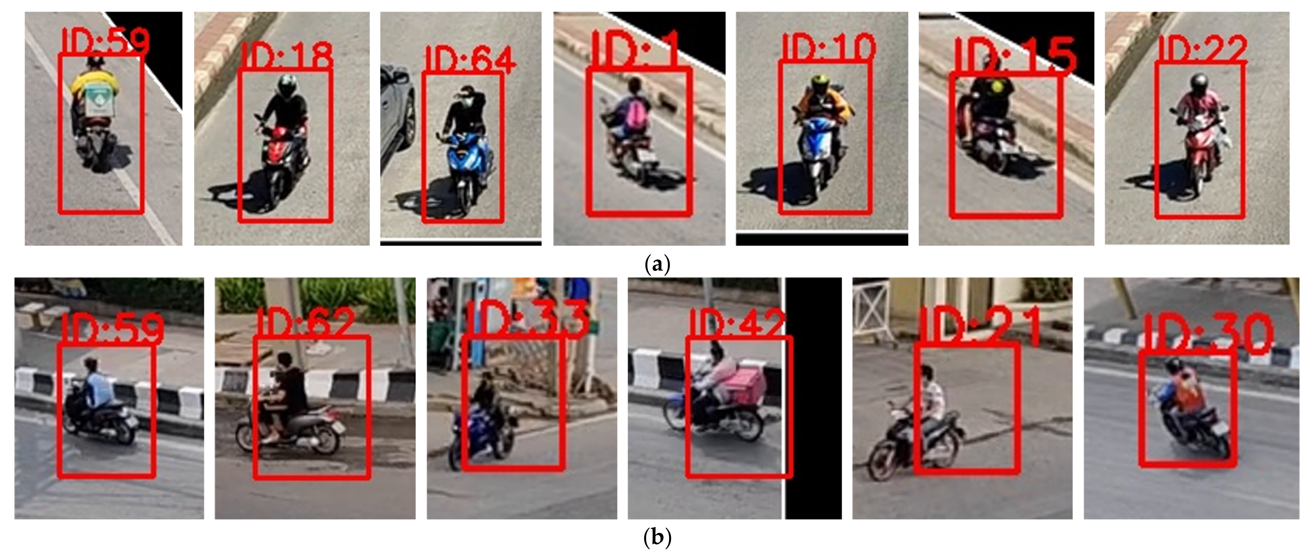
2.4. Inside Boundary Image Capturing Feature

The last sub-system in the WrongWay-LVDC is IBI capturing feature, which captures the moment where the wrong-way driver appears inside the video frame for illegal pieces of evidence. After detecting the vehicles that drive in the wrong direction, the DBDD algorithm will return the summary report containing the counting of the total number of vehicles driving in each direction. Apart from the summary number, we need to capture the image of the wrong driving in the act. The challenging part of this algorithm is the high-speed movement of the vehicles on the road, where we have to find the right moment to capture the clearest and closest shot of that driving vehicle. The proposed algorithm is called the Inside Boundary Image capturing algorithm (IBI Capture). The benefit of this algorithm is to identify the individual driver who drives in the wrong direction and to trace back the evidence of the wrong driving behavior. Noted that in this research, we do not use the driver’s personal information. The experiment of our research is just to test the system’s accuracy and clearness only. The system flow for IBI capturing algorithm is shown in Figure 28.
There are two moving orientations of the road depending on the location and camera angle. To create the IBI capturing algorithm, we need to consider both orientations. The flowchart in Figure 28 shows essential steps and decisions of the proposed IBI capturing algorithm based on different road angle orientations.

2.4.1. Vertical Orientation

The assumption is the vehicle moves upward and downward along the vertical orientation. The vehicle moves closer to the camera when it moves closer to the lower boundary. Thus, the system will capture images of the vehicle that drives in the wrong direction when the vehicle comes closer to the lower boundary.
There are two cases about the vertical orientation that we have concerns about—first, when the wrong driving vehicle is driving downward whereas the correct driving direction is upward. The closest moment to capturing the wrong driving vehicle is when the vehicle is about to leave the lower boundary. Second, when the correct driving direction is downward, and the wrong-way driving vehicle is driving upward. The closest moment to capturing the wrong-way driving vehicle is when the vehicle first appears into the lower boundary. We apply different methods to capture the image based on these two cases.
Using the OpenCV library, the coordinate system will be arranged so that the y-axis value will be flipped from the normal coordinate, as shown in Figure 29.
The method to determine if the wrong-way driving vehicle is going to drive upward or downward is to check with the height of the stopping area reference value and the height of the lower boundary, as shown in the equation below.
W r o n g   w a y   d r i v i n g   d i r e c t i o n = u p w a r d , h e i g h t   o f   r e f e r e n c e   p o i n t < h e i g h t   o f   l o w e r   b o u n d a r y d o w n w a r d ,       h e i g h t   o f   r e f e r e n c e   p o i n t > h e i g h t   o f   l o w e r   b o u n d a r y
In order to find the closest and most precise moment to capture the images, the system requires the y value of the vehicle’s current location (referred to as CY) and the y value of the lower boundary (referred to as YL). For the case when the wrong-way-driving vehicle is driving downward, the system calculates the difference between CY and YL values. The best moment for image capturing is when the difference value of CY and YL is close to zero, meaning that the lower part of the vehicle bounding box is lying on or below the lower boundary line. In such a case, we might not obtain whole components of the vehicles. As shown in an example in Figure 30a, the motorcycle’s front wheel is being blocked by the road lane boundary. Therefore, we set a value of 20 pixels to be the maximum difference value between the CY and YL points to make a screenshot image of the vehicle. The value of 20 pixels has been evaluated as a proper value to leave some distance between the vehicle’s bounding box and the YL. An example of captured images is shown in Figure 30b.
Or the case where the wrong-way driving vehicle is driving upward, the system captures the first frame where the vehicle appears and is detected as wrong-way driving. This screenshot is shown in Figure 31.

2.4.2. Horizontal Orientation

The method for capturing the image in the horizontal orientation selects the frame where the bounding box of the detection is the biggest. The example screenshot of the vehicle driving in the wrong direction in horizontal orientation is shown in Figure 32.

2.5. Framework’s Version

The main purpose of our framework is to let each algorithm and feature executed automatically after one another. Nevertheless, there are some concerns about the system’s performance when it encounters some unusual scenarios. However, we try to design the system so it works best and can provide accurate results even if some unwanted conditions are present. To make it possible, we improved our framework so the user can manually draw and validate the road lane boundary in addition to using the RLB-CCTV and DBDD algorithms. The workflow of the improved framework is shown in Figure 33.

3. Results

We performed many experiments on a number of videos. Based on the outputs, we observed many interesting results, and the more detailed explanations are described in different aspects in the following sections.

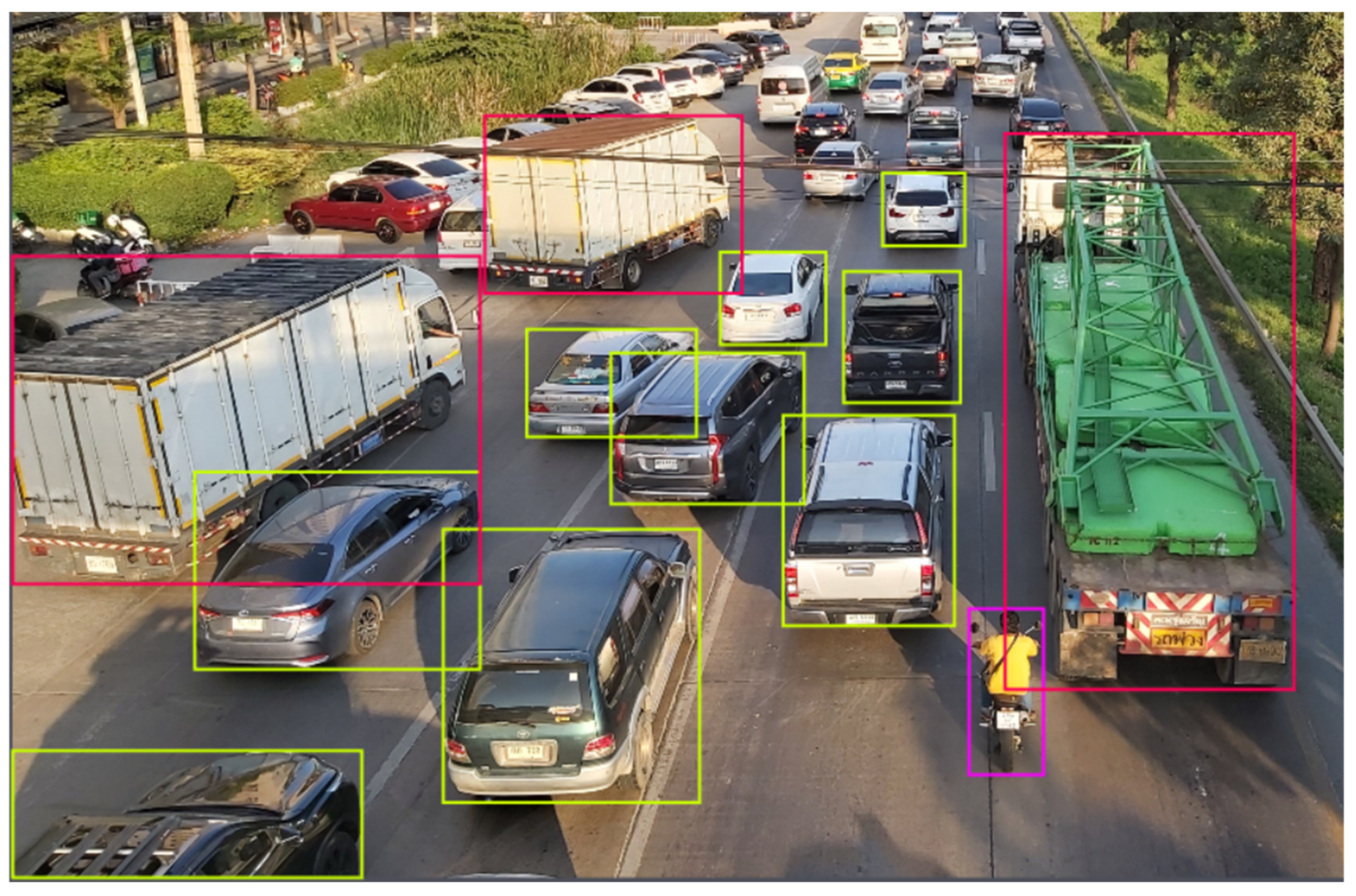
3.1. Object Detection

Our image data set were collected based on various locations and times. The cameras were set to capture images on several skywalks around Bangkok and Pathum Thani province. The sample of captured images is shown in Figure 34. We obtained a total of 437 images for our experiments. To detect the various kind of vehicles on the road, we annotated the objects into three classes: motorcycles, cars, and large vehicles.
As we prepared the dataset and the label, we trained the model with YOLOv4-Tiny. We divided the augmented data set for the trained and validation sets as 80% and 20%, respectively. The total number of images used for the trained model is 1068 images. The result and accuracy of the model after training for motorcycles, cars, and large vehicles are shown in Table 1.
We decided to use YOLOv4 TinyDue due to the requirement that we need a fast algorithm to deploy on an embedded system. However, YOLOv4 Tiny has a trade-off with accuracy compared to other algorithms such as YOLOv4 or YOLOv3. According to Song et al. [42], they used YOLOv3 and achieved up to 87.88% accuracy for mAP. Roszyk et al. [43] obtained the average accuracy of 0.557 for mAP50. Although YOLOv4 or YOLOv3 can provide higher accuracy, these algorithms are inappropriate for real-time detection on an embedded system deployment because of the slow detections. Thus, we select YOLOv4 Tiny, which works best for real-time detection with acceptable high accuracy.

3.2. Result of the Framework

Based on our experimental results, we discovered a high number of motorcycles driving in the wrong direction. The system captured the images from the video in various ranges (e.g., 2 to 5 min). It is important to note that the angle of our captured videos was limited due to the angles of CCTVs on the skywalk. Some angles of the video show the vehicles driving vertically while some are driving horizontally. We used ten videos for our experiments.

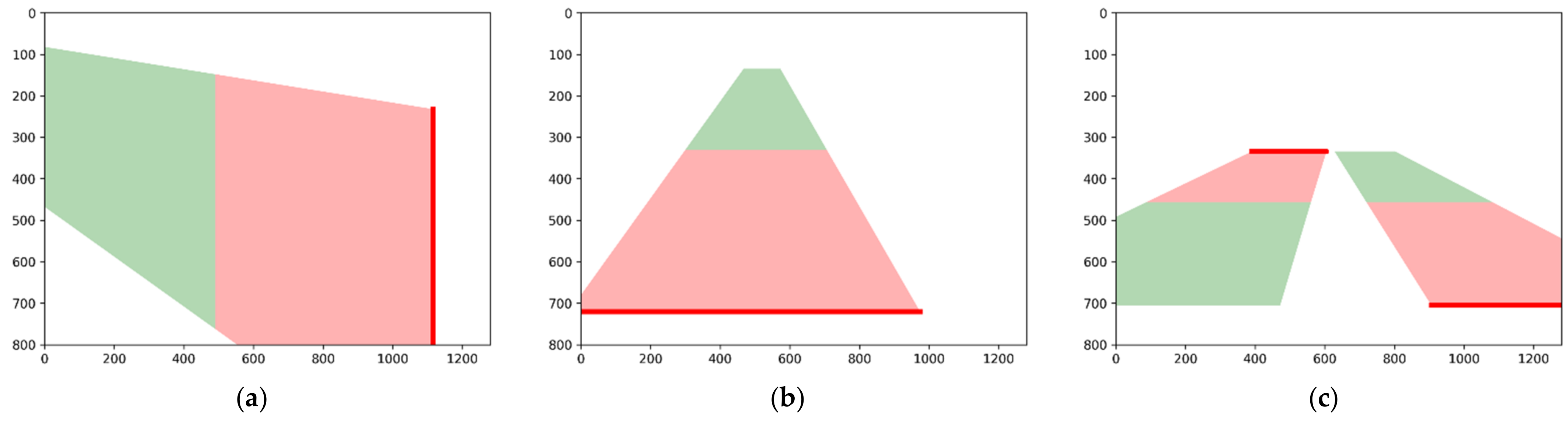
3.2.1. Improved RLB-CCTV Algorithm

After collecting several videos from many locations, we tested the videos with our proposed algorithm to detect the road lane boundary. Some video contains one road, and some contain two roads. Our system returned satisfactory results of road lane boundary detections. Some of the results are shown in Figure 35.

3.2.2. DBDD Algorithm

In the DBDD algorithm, there are two steps to proceed: validation and detection steps. First, we show the result of the system after validating the correct moving direction by finding the start, stop areas, and reference points. Table 2 shows the result from the DBDD validation step, where it shows the information on the number of the start and stop points in each area.
As we use this configuration from the validation step and run the video to let the system determines the moving direction of each vehicle driving inside the lane boundary. The advantage of DBDD over our last proposed system MBCDD is that DBDD requires a shorter video length in the validation step on an embedded system. Both algorithms have similar accuracy as we tested them with the same dataset. However, after we tested the system on edge devices, MBCDD returned a lower performance than DBDD in the validation step. For testing on the Jetson Nano, DBDD requires only short videos (one minute at maximum) for the validation step to correctly validate the correct moving direction of vehicles in each lane. On the other hand, MBCDD requires a thrice longer length of video than DBDD to validate the correct vehicles’ moving directions. Based on the testing results, we can see the advantage of DBDD and its performance on edge devices.
The next step after the validation step is the detection step. In the detection step, the system determines and detects each lane for the correct and wrong-way driving of vehicles. The algorithm is shown in Table 3. We tested the system on both a personal computer and an embedded system (Jetson Nano). The results of detection are quite similar and close to the ground truth. There was some slight error in detection due to the accuracy of the object detection and tracking system. We evaluated the accuracy of our proposed system using ten videos; the accuracies were 95.225% when running on a personal computer and 94.663% on Jetson Nano, respectively. The limited resources on the Jetson Nano caused the difference in the accuracy when running object detection and tracking algorithms. The average FPS on the Jetson Nano was approximately 24 FPS, which is suitable for real-time detection.
Figure 36 shows the screenshot of the detection process while the system is detecting the wrong-way driving vehicle on a video with vertical orientation. The system can track and detect vehicles accurately.

3.2.3. IBI Capturing Feature

The IBI capturing feature algorithm is used to capture the most precise image, capturing the closest moment where the vehicle comes closest to the camera. Figure 36 shows screenshot images cropped to the size of a vehicle that drives in the wrong direction. Figure 37a,b show the example captured images with IBI capturing features when vehicles are driving in vertical and horizontal orientations, respectively. As we mentioned in the problem statement and the motivation for this research, the motorcycle is the major type of vehicle that often be found driving in illegal directions on road lanes in Thailand. Therefore, we only focus on detecting the motorcycles in this research. Although there are some cases where other types of vehicles (e.g., car or truck) are found when driving in the wrong direction, we do not have sufficient images of those cases captured in our video records for the experiments.

4. Discussion

4.1. Limitations

The scope of our research is to detect the road lane and be able to implement the system onto a real-time embedded system, such as a Jetson Nano. Therefore, there are three limitations we would like to discuss for future improvements.
The first limitation is running the system using limited resources on the Jetson Nano. The Jetson Nano is an effective embedded system that can perform image processing tasks. To achieve higher FPS, we have to resolve several issues to make our algorithms on the Jetson Nano work best for the real-time processing system. For example, we must narrow the road boundary to make it smaller for processing on the Jetson Nano. If we use the original boundary size, the system will take more computing time to compute a large area. Therefore, we decided to reduce the size of the road boundary after detecting it with the Road-CCTV algorithm.
The second limitation is about various road conditions. It is challenging to detect all types of roads in the system. There are many factors that influence the accuracy of the RLB-CCTV and DBDD algorithms. For example, when there are objects blocking the road lane, the system may not detect the road lane accurately. We need to consider several conditions for improving our road lane detection algorithm. In addition, the current system can only detect the road lane with a straight line in vertical or horizontal orientations; we would like to improve our approach to handle the curved road in future work.
The last limitation is the capability to validate the correct driving direction regarding the speed and accuracy of the MBCDD. According to our experimental results, the algorithm provided high accuracy wrong-way driving detection. However, there are some aspects in the validation step that the algorithm remains at a weak point. We would like to have a shorter time validating the correct direction on a road boundary with great accuracy. Thus, the length of the validating video should be shortened for time reduction. However, the challenging part is, can a short validating video produce a threshold value with enough accuracy, especially for the validation on the embedded system? We tested this idea by trimming the video length to 1000 frames, 2000 frames, and 3000 frames. In Table 4, we tested our algorithm with the stated configuration of the video’s lengths for the validation step on Jetson Nano.
As shown in Table 4, the threshold values increase according to the number of video lengths. Figure 38 shows the detected vehicle movements used in the validation step. The higher number of frames from the video length increases the accuracy of the majority direction most vehicles are moving toward.
Table 4 shows varying, different results. As we manually counted, the ground truth of the number of vehicles is 51 and 15 for the correct-way and wrong-way driving, respectively. To compare the error in both correct-way driving vehicle and wrong-way driving vehicle columns in Table 4 with the ground truth, the 1000 frames, 2000 frames, and 3000 frames produce seven, four, and one miscounted vehicles, respectively. With this information, we can conclude that the minimum number of frame lengths to use in the validation step for MBCDD running on Jetson Nano is 3000 frames, which takes around 7.5 min to validate the direction, while the actual video run times for 3000 frames should be only around 1 min and 40 s. For DBDD, the validation step is simpler where the video frame length at 1000 frames already produces an accurate validation result. With these concerns, we decided to use our proposed DBDD algorithm as part of our WrongWay-LVDC framework.

4.2. Challenging Constraints

To test our proposed algorithms and whether they would handle various scenarios and constraints, we have gathered possible scenarios that would happen while running the framework. There are four cases of challenging constraints. The first case is the resolution of the CCTV cameras. As we could not directly access the CCTV camera for the video, in this research, we imitated the CCTV camera angle and recorded the video using the smartphone. The videos we received from the smartphone have a resolution of 1920 pixels in width and 1080 pixels in height. We converted the resolution to 1280 pixels in width and 720 pixels in height for faster processing. As we checked the resolution of the CCTV, the converted resolution of the input video is equivalent to a 720p HD video from CCTV. There are many several higher resolutions of video that are collected from CCTV. However, as long as the resolution of the input video from the actual CCTV is greater than 1280 × 720 pixels, the input video should be compatible with our system.
The second case is when there is heavy traffic. During rush hours, we often face bad traffic, where all vehicles on the road move slowly or do not move for a certain time. As the system’s default requires one minute video for the validation part, in the case of traffic jams, the distances of each moving vehicle in the video might be too short, and the system might not obtain the significant information to validate the correct direction of a road lane. In the case that the vehicle is moving slowly in the video length of one minute, for the MBCDD algorithm, this case would not affect the efficiency of the system to validate the correct moving direction because even the tiny direction movement is sufficient for the system to understand the majority moving direction of all vehicles. However, this will severely affect the validation part of the DBDD algorithm since the algorithm will divide the road into two areas, the start and stop areas. If the vehicles do not have enough time, within one minute, to drive across from the start area to the stop area, the system will fail to validate the correct direction. However, this situation can be solved by increasing the time for the validation video, depending on the time of the day of the video that is selected to be the validation video. The system should avoid using the video during rush hour to validate the correct direction. If it is unavoidable, the longer length of the video, such as 3 or 5 min, should be used to validate instead, as this will be a solution for the system to obtain more accuracy in direction validation.
The third case is when the vehicle is driving too fast. Oppositely to the previous case, we also consider the capability of the system to detect fast-moving 64 vehicles. The collected video has a resolution of 30 frames per second. When the vehicle is driving too fast and appears in only one frame in the video, the system will not be able to track the moving direction due to the low information provided. Detection is possible when a fast-moving vehicle appears for at least two frames inside a video. In this case, there will be two challenges for our proposed systems: tracking capability and direction validation.
For direction validation, this might be a challenge to detect the moving direction of a vehicle that appears inside the video for two frames. However, our algorithms can detect and specify the moving direction even in a few frames that a vehicle appears in. Both of our wrong-way driving detectors (MBCDD and DBDD) only require two vehicle locations to determine the vehicle’s distance and moving angle. With this idea, we can conclude that even if the vehicle is moving very fast, with only two frames, it appears our algorithms can verify the moving direction of that vehicle.
We tested our system using short video clips of around 3 to 5 min. We have another concern when using longer video clips, which might affect the detection performance. Therefore, the fourth challenging case is using the longer length of the video inputs. As we run the wrong-way driver detection on PC, the speed is up to 80 FPS in a normal traffic scenario. With the high performance on PC, the trend of detecting speed will not drop below the real-time speed, which is around 30 FPS, even if the input video is very long. However, running a long video on a small embedded is a major concern because the embedded system has limited resources, and it always becomes easier to obtain a high temperature and decrease the detection performance. As we tested our system on the Jetson Nano, the average speed was around 24 FPS. In the scenario where the traffic is heavy on the testing video, the speed may drop below 20 FPS. Therefore, there are many factors that would affect the speed of wrong-way driver detection on an embedded system. There are potential solutions that support wrong-way driver detection. First, keep the embedded system’s temperature low and avoid the overheat condition while detecting. Second, skipping the frame of detection for the input video. If the device detects all vehicles every frame, it will consume excessive energy and would slow down the process. Lastly, turning off the interface display while running the system reduces power consumption. With these approaches, the detection on embedded systems would remain in a good performance detecting long video clips.

5. Conclusions

In our research, we proposed the WrongWay-LVDC framework, which consists of three proposed sub-systems; improved road lane boundary detection from CCTV (improved RLB-CCTV), Distance-Based Direction Detection (DBDD), and Inside Boundary Image Capturing (IBI capturing). Each of these sub-systems will run after one another synchronously and automatically. This seamless pipeline flow makes it convenient and functional to use in a broad area. Furthermore, we can deploy our framework on an embedded system at a real-time average speed of 24 FPS. The obtained accuracies are 95.23% while running on a personal computer and 94.66% on the embedded system. We can conclude that the proposed framework can provide high accuracy and speed performance for an IoT purpose. For future work, this research has a high potential to be improved in several aspects to enhance the algorithms to handle several cases of road conditions. For example, the improved RLB-CCTV should be able to detect various road conditions such as curve line roads, roads with objects blocking on the side, and roads with projected shadows. Moreover, new features can be added to this framework based on improving speed detection and detecting traffic density levels.

Author Contributions

Conceptualization, P.S., C.C. and S.U.; methodology, P.S., C.C. and S.U.; software, P.S.; validation, P.S., C.C. and S.U.; formal analysis, P.S.; investigation, S.U.; resources, C.C.; data curation, P.S. and S.U.; writing—original draft preparation, P.S. and S.U.; writing—review and editing, C.C. and S.U.; visualization, P.S.; supervision, C.C., S.U. and H.N. All authors have read and agreed to the published version of the manuscript.

Funding

This research received no external funding.

Institutional Review Board Statement

Not applicable.

Informed Consent Statement

Not applicable.

Data Availability Statement

Not applicable.

Acknowledgments

This research is supported by Thailand Advanced Institute of Science and Technology (TAIST), National Science and Technology Development Agency (NSTDA), Tokyo Institute of Technology, Sirindhorn International Institute of Technology (SIIT), Thammasat University (TU) under the TAIST Tokyo Tech Program.

Conflicts of Interest

The authors declare no conflict of interest.

References

  1. Road Traffic Injuries. Available online: https://www.who.int/news-room/fact-sheets/detail/road-traffic-injuries#:~:text=Road%20traffic%20injuries%20are%20the,pedestrians%2C%20cyclists%2C%20and%20motorcyclists (accessed on 6 August 2022).
  2. Thai RSC. Available online: https://www.thairsc.com (accessed on 16 March 2022).
  3. World Life Expectancy, Road Traffic Accidents. Available online: https://www.worldlifeexpectancy.com/cause-of-death/road-traffic-accidents/by-country/ (accessed on 16 March 2022).
  4. 5 Major Areas in Bangkok that Still Have Wrong-Way Driving Motorcycles. Available online: https://www.pptvhd36.com/news/%E0%B8%9B%E0%B8%A3%E0%B8%B0%E0%B9%80%E0%B8%94%E0%B9%87%E0% (accessed on 16 March 2022).
  5. Usmankhujaev, S.; Baydadaev, S.; Woo, K.J. Real-Time, Deep Learning Based Wrong Direction Detection. Appl. Sci. 2020, 10, 2453. [Google Scholar] [CrossRef]
  6. Montella, C. The Kalman Filter and Related Algorithms: A Literature Review. 2011. Available online: https://www.researchgate.net/publication/236897001_The_Kalman_Filter_and_Related_Algorithms_A_Literature_Review (accessed on 17 July 2022).
  7. Joseph, R.; Ali, F. YOLOv3: An Incremental Improvement. arXiv 2018, arXiv:1804.02767. [Google Scholar]
  8. Monteiro, G.; Ribeiro, M.; Marcos, J.; Batista, J. Wrongway Drivers Detection Based on Optical Flow. IEEE Int. Conf. Image Process. 2007, 5, 141–144. [Google Scholar] [CrossRef]
  9. Rahman, Z.; Ami, A.M.; Ullah, M.A. A Real-Time Wrong-Way Vehicle Detection Based on YOLO and Centroid Tracking. In Proceedings of the 2020 IEEE Region 10 Symposium (TENSYMP), Dhaka, Bangladesh, 5–7 June 2020; pp. 916–920. [Google Scholar] [CrossRef]
  10. Pudasaini, D.; Abhari, A. Scalable Object Detection, Tracking and Pattern Recognition Model Using Edge Computing. In Proceedings of the 2020 Spring Simulation Conference (SpringSim), Fairfax, VA, USA, 18–21 May 2020; pp. 1–11. [Google Scholar] [CrossRef]
  11. Gu, H.; Ge, Z.; Cao, E.; Chen, M.; Wei, T.; Fu, X.; Hu, S. A Collaborative and Sustainable Edge-Cloud Architecture for Object Tracking with Convolutional Siamese Networks. IEEE Trans. Sustain. Comput. 2021, 6, 144–154. [Google Scholar] [CrossRef]
  12. Coral. Available online: https://coral.ai/ (accessed on 16 March 2022).
  13. NVIDIA Jetson. Available online: https://developer.nvidia.com/embedded/jetson-modules (accessed on 16 March 2022).
  14. Raspberry Pi Foundation. Available online: https://www.raspberrypi.org/ (accessed on 16 March 2022).
  15. Zualkernan, I.; Dhou, S.; Judas, J.; Sajun, A.R.; Gomez, B.R.; Hussain, L.A. An IoT System Using Deep Learning to Classify Camera Trap Images on the Edge. Computers 2022, 11, 13. [Google Scholar] [CrossRef]
  16. Jetson Nano Developer Kit. Available online: https://developer.nvidia.com/embedded/jetson-nano-developer-kit (accessed on 16 March 2022).
  17. Liu, L.; Chen, X.; Zhu, S.; Tan, P. CondLaneNet: A Top-to-down Lane Detection Framework Based on Conditional Convolution. In Proceedings of the IEEE/CVF International Conference on Computer Vision (ICCV), Montreal, QC, Canada, 11–17 October 2021; pp. 3773–3782. [Google Scholar]
  18. Chen, L.; Xu, X.; Pan, L.; Cao, J.; Li, X. Real-time lane detection model based on non bottleneck skip residual connections and attention pyramids. PLoS ONE 2021, 16, e0252755. [Google Scholar] [CrossRef] [PubMed]
  19. Andrei, M.-A.; Boiangiu, C.-A.; Tarbă, N.; Voncilă, M.-L. Robust Lane Detection and Tracking Algorithm for Steering Assist Systems. Machines 2022, 10, 10. [Google Scholar] [CrossRef]
  20. Sharma, A.; Kumar, M.; Kumar, R. Lane detection using Python. In Proceedings of the 2021 3rd International Conference on Advances in Computing, Communication Control and Networking (ICAC3N), Greater Noida, India, 17–18 December 2021; pp. 88–90. [Google Scholar]
  21. Rakotondrajao, F.; Jangsamsi, K. Road Boundary Detection for Straight Lane Lines Using Automatic Inverse Perspective Mapping. In Proceedings of the 2019 International Symposium on Intelligent Signal Processing and Communication Systems (ISPACS), Taipei, Taiwan, 3–6 December 2019; pp. 1–2. [Google Scholar] [CrossRef]
  22. Franco, F.; Santos, M.M.D.; Yoshino, R.T.; Yoshioka, L.R.; Justo, J.F. ROADLANE—The Modular Framework to Support Recognition Algorithms of Road Lane Markings. Appl. Sci. 2021, 11, 10783. [Google Scholar] [CrossRef]
  23. Ghazali, K.; Xiao, R.; Ma, J. Road Lane Detection Using H-Maxima and Improved Hough Transform. In Proceedings of the 2012 Fourth International Conference on Computational Intelligence, Modelling and Simulation, Kuantan, Malaysia, 25–27 September 2012; pp. 205–208. [Google Scholar] [CrossRef]
  24. Farag, W.; Saleh, Z. Road Lane-Lines Detection in Real-Time for Advanced Driving Assistance Systems. In Proceedings of the 2018 International Conference on Innovation and Intelligence for Informatics, Computing, and Technologies (3ICT), Sakhier, Bahrain, 18–20 November 2018; pp. 1–8. [Google Scholar] [CrossRef]
  25. Python. Available online: https://www.python.org/ (accessed on 6 August 2022).
  26. Linux. Available online: https://www.linux.com/ (accessed on 6 August 2022).
  27. OpenCV. Available online: https://opencv.org/ (accessed on 16 March 2022).
  28. Bochkovskiy, A.; Wang, C.Y.; Liao, H.Y. YOLOv4: Optimal Speed and Accuracy of Object Detection. arXiv 2020, arXiv:2004.10934. [Google Scholar]
  29. FastMOT: High-Performance Multiple Object Tracking Based on Deep SORT and KLT. Available online: https://github.com/GeekAlexis/FastMOT (accessed on 16 March 2022).
  30. Canny, J. A Computational Approach to Edge Detection. IEEE Trans. Pattern Anal. Mach. Intell. 1986, 8, 679–698. [Google Scholar] [CrossRef] [PubMed]
  31. Duda, R.O.; Hart, P.E. Use of the Hough Transformation to Detect Lines and Curves in Pictures. Commun. ACM 1972, 15, 11–15. [Google Scholar] [CrossRef]
  32. Gedraite, E.; Hadad, M. Investigation on the effect of a Gaussian Blur in image filtering and segmentation. In Proceedings of the ELMAR-2011, Zadar, Croatia, 14–16 September 2011; pp. 393–396. [Google Scholar]
  33. Suttiponpisarn, P.; Charnsripinyo, C.; Usanavasin, S.; Nakahara, H. An Enhanced System for Wrong-Way Driving Vehicle Detection with Road Boundary Detection Algorithm. In Proceedings of the 2022 International Conference on Industry Science and Computer Sciences Innovation, Oporto, Portugal, 9–11 March 2022. in press. [Google Scholar]
  34. ImageStat Module. Available online: https://pillow.readthedocs.io/en/stable/reference/ImageStat.html (accessed on 17 March 2022).
  35. HSL and HSV. Available online: https://en.wikipedia.org/wiki/HSL_and_HSV (accessed on 17 March 2022).
  36. Yadav, G.; Maheshwari, S.; Agarwal, A. Contrast limited adaptive histogram equalization based enhancement for real time video system. In Proceedings of the 2014 International Conference on Advances in Computing, Communications and Informatics (ICACCI), Delhi, India, 24–27 September 2014; pp. 2392–2397. [Google Scholar] [CrossRef]
  37. Patel, O.; Maravi, Y.; Sharma, S. A Comparative Study of Histogram Equalization Based Image Enhancement Techniques for Brightness Preservation and Contrast Enhancement. Signal Image Process. Int. J. 2013, 4, 11–25. [Google Scholar] [CrossRef]
  38. Sharif, M. A new approach to compute convex hull. Innov. Syst. Des. Eng. 2011, 2, 187–193. [Google Scholar]
  39. OpenCV Bitwise AND, OR, XOR, and NOT. Available online: https://pyimagesearch.com/2021/01/19/opencv-bitwise-and-or-xor-and-not/ (accessed on 17 March 2022).
  40. The Shapely User Manual. Available online: https://shapely.readthedocs.io/en/stable/manual.html (accessed on 17 March 2022).
  41. Suttiponpisarn, P.; Charnsripinyo, C.; Usanavasin, S.; Nakahara, H. Detection of Wrong Direction Vehicles on Two-Way Traffic. In Proceedings of the 13th International Conference on Knowledge and Systems Engineering, Bangkok, Thailand, 10–12 November 2021. [Google Scholar]
  42. Song, H.; Liang, H.; Li, H.; Dai, Z.; Yun, X. Vision-based vehicle detection and counting system using deep learning in highway scenes. Eur. Transp. Res. Rev. 2019, 11, 51. [Google Scholar] [CrossRef]
  43. Roszyk, K.; Nowicki, M.R.; Skrzypczyński, P. Adopting the YOLOv4 Architecture for Low-Latency Multispectral Pedestrian Detection in Autonomous Driving. Sensors 2022, 22, 1082. [Google Scholar] [CrossRef] [PubMed]
Figure 1. Image evidence of many motorcycles driving in the wrong direction on Paholyothin road, in front of Bangkok University.
Sustainability 14 10232 g001
Figure 2. WrongWay-LVDC’s framework flow.
Sustainability 14 10232 g002
Figure 4. System flow on the method to obtain the vehicle information and image.
Sustainability 14 10232 g004
Figure 5. Vehicle Information Plotting.
Sustainability 14 10232 g005
Figure 6. Camera view of CCTV (a) vertical orientation; (b) vertical orientation; (c) horizontal orientation.
Sustainability 14 10232 g006
Figure 7. System flow of Improved RLB-CCTV.
Sustainability 14 10232 g007
Figure 8. The vehicle information was obtained after detecting and tracking all vehicles in the video for one minute. (a) Horizontal orientation; (b) Vertical orientation; (c) Vertical orientation with two roads.
Sustainability 14 10232 g008
Figure 9. System Flow of Orientation Decision Step.
Sustainability 14 10232 g009
Figure 10. Step to obtain the vectors to find the angle (a) Obtain vehicle information as an input; (b) Set the lower point to be P1 and the upper point to be P2; (c) Draw a vector to the right where the initial point is P1; (d) Obtain the vehicle movement vector from P1 and P2; (e) Find the angle in degree.
Sustainability 14 10232 g010
Figure 11. All possible vectors and angles.
Sustainability 14 10232 g011
Figure 12. Angle value histogram plot. (a) Horizontal orientation; (b) Vertical orientation; (c) Vertical orientation with two lanes.
Sustainability 14 10232 g012
Figure 13. System Flow of Image Pre-processing Step.
Sustainability 14 10232 g013
Figure 14. Adjust the brightness on the input image (a) Horizontal orientation; (b) Vertical orientation; (c) Vertical orientation with two lanes. Apply CLAHE and Gaussian Blur (d) Horizontal orientation; (e) Vertical orientation; (f) Vertical orientation with two lanes.
Sustainability 14 10232 g014
Figure 15. Apply Histogram Equalization. (a) Horizontal orientation; (b) Vertical orientation; (c) Vertical orientation with two lanes. Apply Canny edge detection (d) Horizontal orientation; (e) Vertical orientation; (f) Vertical orientation with two lanes.
Sustainability 14 10232 g015
Figure 16. System flow of Area of Interest step.
Sustainability 14 10232 g016
Figure 17. Apply convex hull to wrap around all start and stop points from vehicle information. (a) Horizontal orientation; (b) Vertical orientation; (c) Vertical orientation with two lanes. Expand the edge of the convex hull shape (d) Horizontal orientation; (e) Vertical orientation; (f) Vertical orientation with two lanes.
Sustainability 14 10232 g017
Figure 18. Apply a bitwise mask between the area of interest and the final output from the image pre-processing step. (a) Horizontal orientation; (b) Vertical orientation; (c) Vertical orientation with two lanes. Remove the upper and lower boundaries (d) Horizontal orientation; (e) Vertical orientation; (f) Vertical orientation with two lanes.
Sustainability 14 10232 g018
Figure 22. Final output; (a) Horizontal orientation; (b) Vertical orientation; (c) Vertical orientation with two lanes.
Sustainability 14 10232 g022
Figure 23. System Flow of DBDD.
Sustainability 14 10232 g023
Figure 24. Overlay all points from vehicle information on the areas; (a) Horizontal orientation; (b) Vertical orientation; (c) Vertical orientation with two lanes. Overlay start points from vehicle information on the areas (d) Horizontal orientation; (e) Vertical orientation; (f) Vertical orientation with two lanes. Overlay stop points from vehicle information on the areas; (g) Horizontal orientation; (h) Vertical orientation; (i) Vertical orientation with two lanes.
Sustainability 14 10232 g024
Figure 25. Label the area and obtain the stopping reference point; (a) Horizontal orientation with a stop area on the right; (b) Vertical orientation with a stop area on the bottom; (c) Vertical orientation with two lanes with opposite driving directions.
Sustainability 14 10232 g025
Figure 26. Length of detected road boundary from the improved RLB-CCTV algorithm; (a) Vertical orientation; (b) Horizontal orientation.
Sustainability 14 10232 g026
Figure 27. The road boundaries are cropped for a range of 3/10 to 7/10; (a) Horizontal orientation; (b) Vertical orientation; (c) Vertical orientation with two lanes.
Sustainability 14 10232 g027
Figure 28. System flow of IBI capturing algorithm.
Sustainability 14 10232 g028
Figure 29. Image coordinate system.
Sustainability 14 10232 g029
Figure 30. (a) The screenshots when the CY bounding box is lower than YL; (b) The screenshots when the CY bounding box is above YL by 20 pixels.
Sustainability 14 10232 g030
Figure 31. The screenshots when the wrong-way driving vehicle is driving upward.
Sustainability 14 10232 g031
Figure 32. The screenshots when capturing vehicles driving in the wrong direction in the vertical oriented video.
Sustainability 14 10232 g032
Figure 33. System flow for different framework’s versions.
Sustainability 14 10232 g033
Figure 34. Labeling the dataset with three classes: Motorcycle, car, and large vehicle.
Sustainability 14 10232 g034
Figure 35. Output images with road boundaries using the improved RLB-CCTV algorithm.
Sustainability 14 10232 g035
Figure 36. Screenshot of the DBDD algorithm while detecting vehicles driving in the correct and wrong direction.
Sustainability 14 10232 g036
Figure 37. Output images of the wrong-way driving vehicles using the IBI capturing feature. (a) Vertical orientation road; (b) Horizontal orientation road.
Sustainability 14 10232 g037
Figure 38. Detected vehicle movements (a) 1000 frame length (b) 2000 frame length (c) 3000 frame length.
Sustainability 14 10232 g038
Table 1. Accuracy of the YOLOv4 Tiny model.
ParametersAPmAP
MotorcycleCarBig Vehicle
Results71.89%78.0%86.25%78.71%
Table 2. The number of start and stop points on each divided area of the road boundary.
VideoLengthAreaNumber of PointsArea Type
StartStopPredictionGround Truth
12:12 minArea 1095StopStop
Area 25035StartStart
Area 3232StartStart
Area 4253StopStop
23:01 minArea 1028StopStop
Area 2181StartStart
Area 3210StartStart
Area 4023StopStop
35:00 minArea 14119StopStop
Area 26840StartStart
42:31 minArea 1264StopStop
Area 24631StartStart
52:59 minArea 111137StartStart
Area 22194StopStop
62:04 minArea 110035StartStart
Area 24228StopStop
74:07 minArea 17234StartStart
Area 20151StopStop
82:00 minArea 1388StopStop
Area 24335StartStart
92:03 minArea 1071StopStop
Area 25016StartStart
102:02 minArea 1341StopStop
Area 210521StartStart
Table 3. Numbers of motorcycles were detected as wrong-way and correct-way driving using DBDD.
VideoLengthLaneGround TruthComputerEmbedded System
Correct
Driving
Wrong
Driving
Correct
Driving
Wrong
Driving
Correct
Driving
Wrong
Driving
FPS
12:12 min191919122
2605061
23:01 min180907023
2302030
35:00 min151155115491727
42:31 min120619619627
52:59 min144446547318
62:04 min126525526519
74:07 min170168168126
82:00 min125102611281025
92:03 min132229233232
102:02 min113514612629
Table 4. MBCDD algorithm in the validation step on Jetson Nano.
Video Length (Frame)ValidationDetection
STDThresholdTime Taken
(Seconds)
Speed
(FPS)
Correct-Way
Driving Vehicle
Wrong-Way
Driving Vehicle
Speed
(FPS)
10006.0530174751823
20006.13073037521220
30006.498144507521520
Publisher’s Note: MDPI stays neutral with regard to jurisdictional claims in published maps and institutional affiliations.

