
Investigation of Spatio–Temporal Changes in Land Use and Heat Stress Indices over Jaipur City Using Geospatial Techniques


Abstract
:1. Introduction
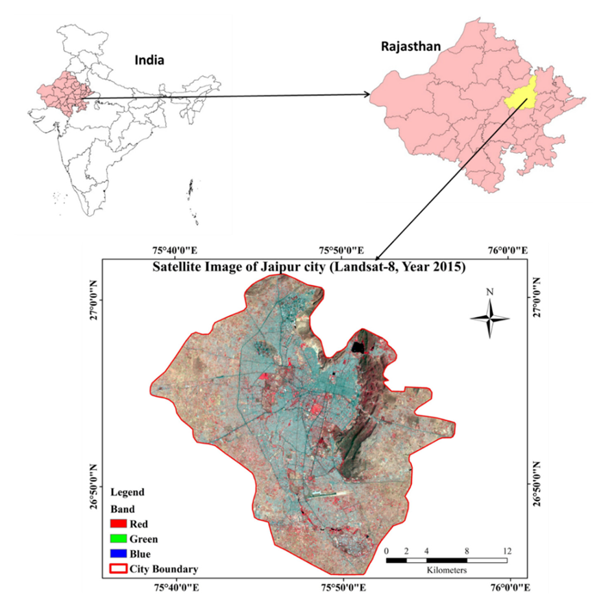
2. Study Area Description
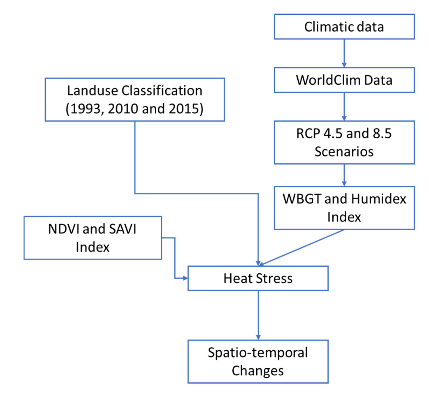
3. Materials and Methods
3.1. Image Classification and Accuracy Assessment
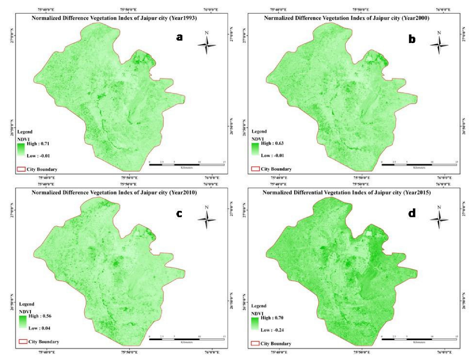
3.2. Normalized Difference Vegetation Index (NDVI)
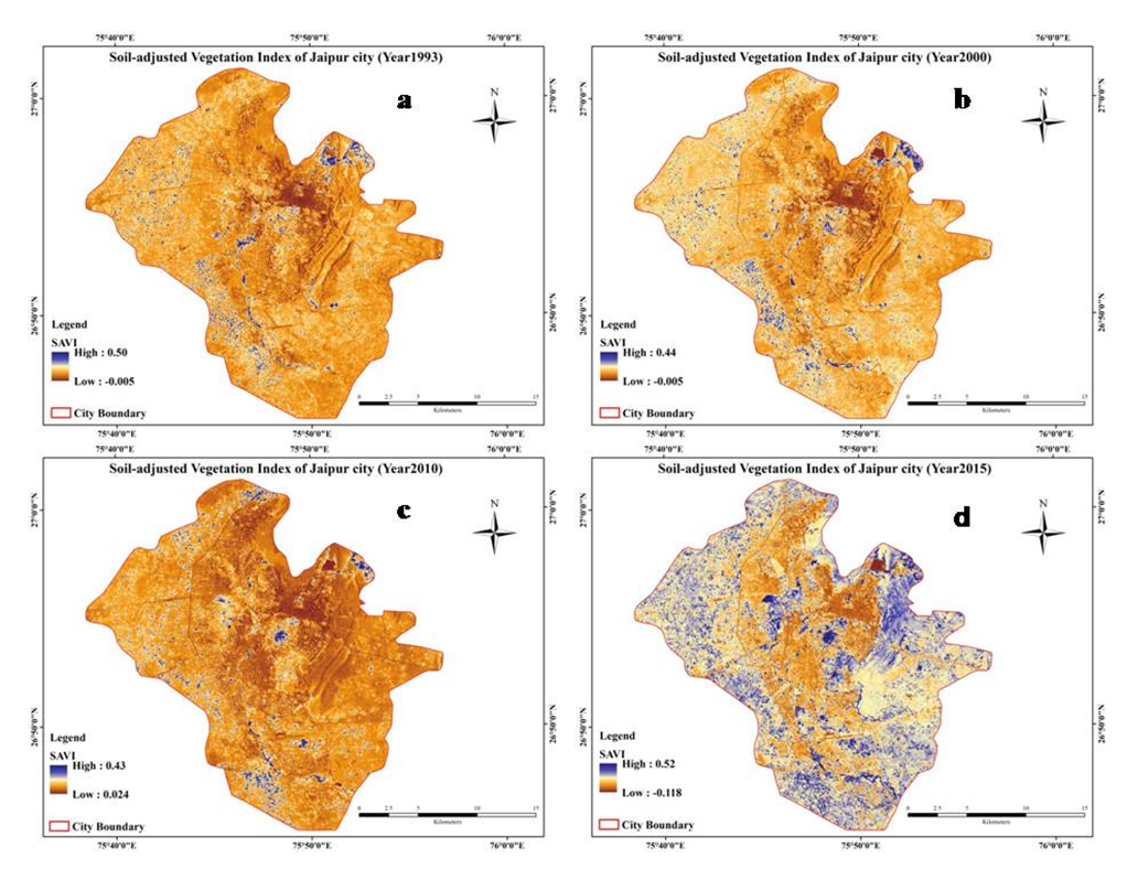
3.3. Soil-Adjusted Vegetation Index Calculate (SAVI)
4. Results and Discussions
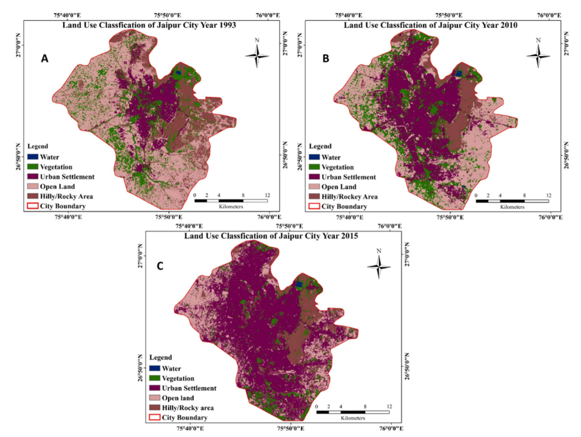
4.1. Land Used Classification
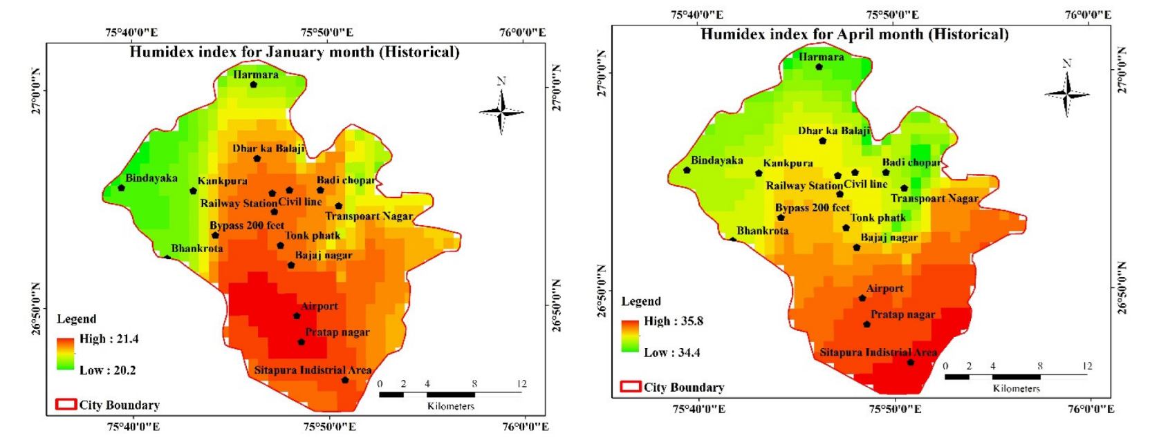
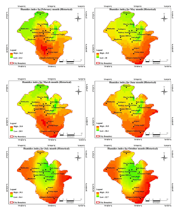
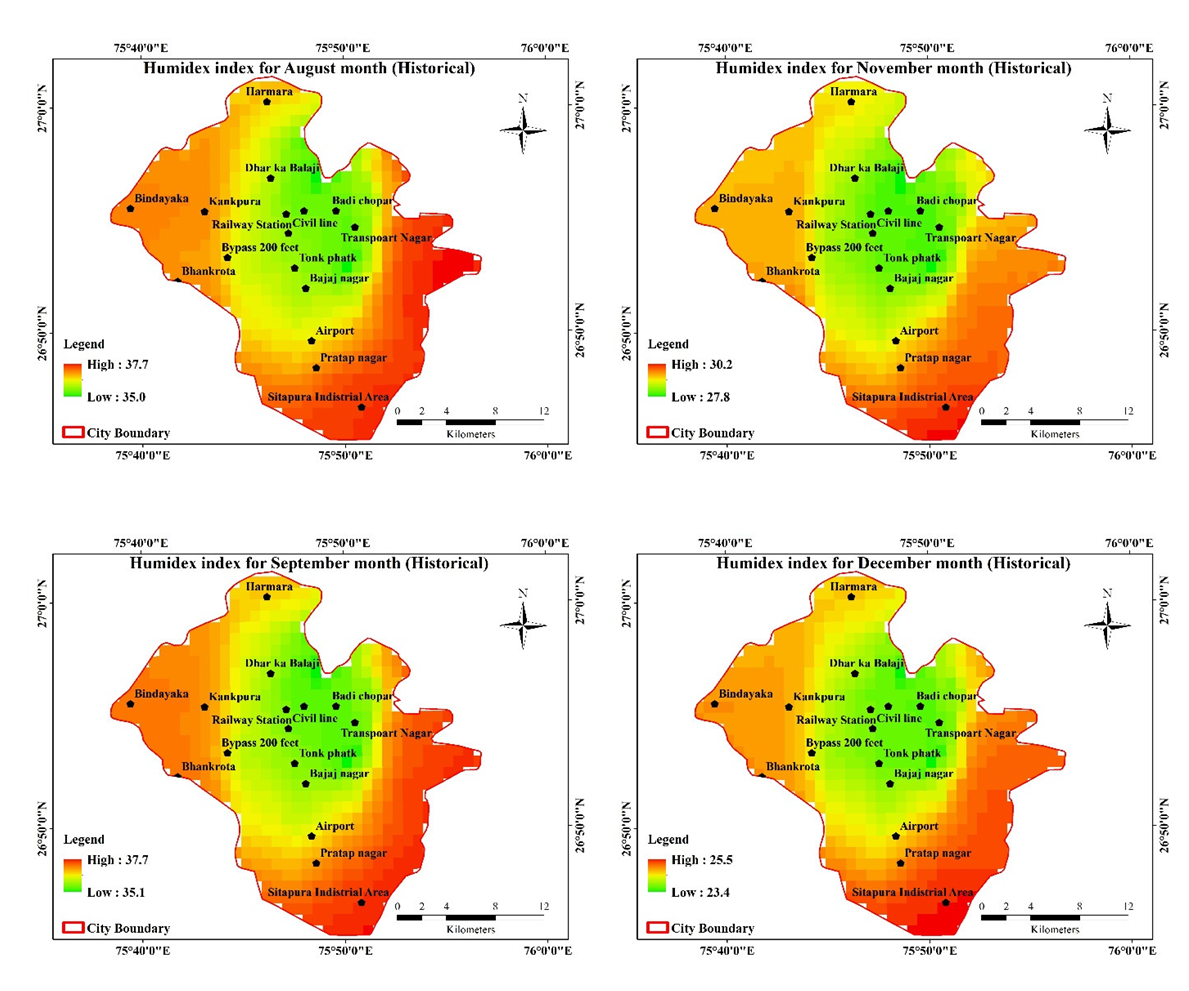
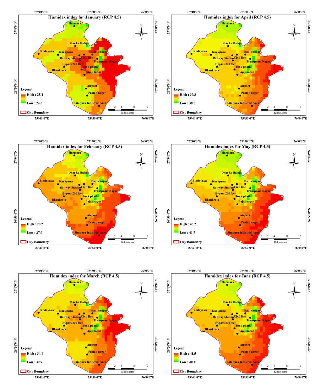
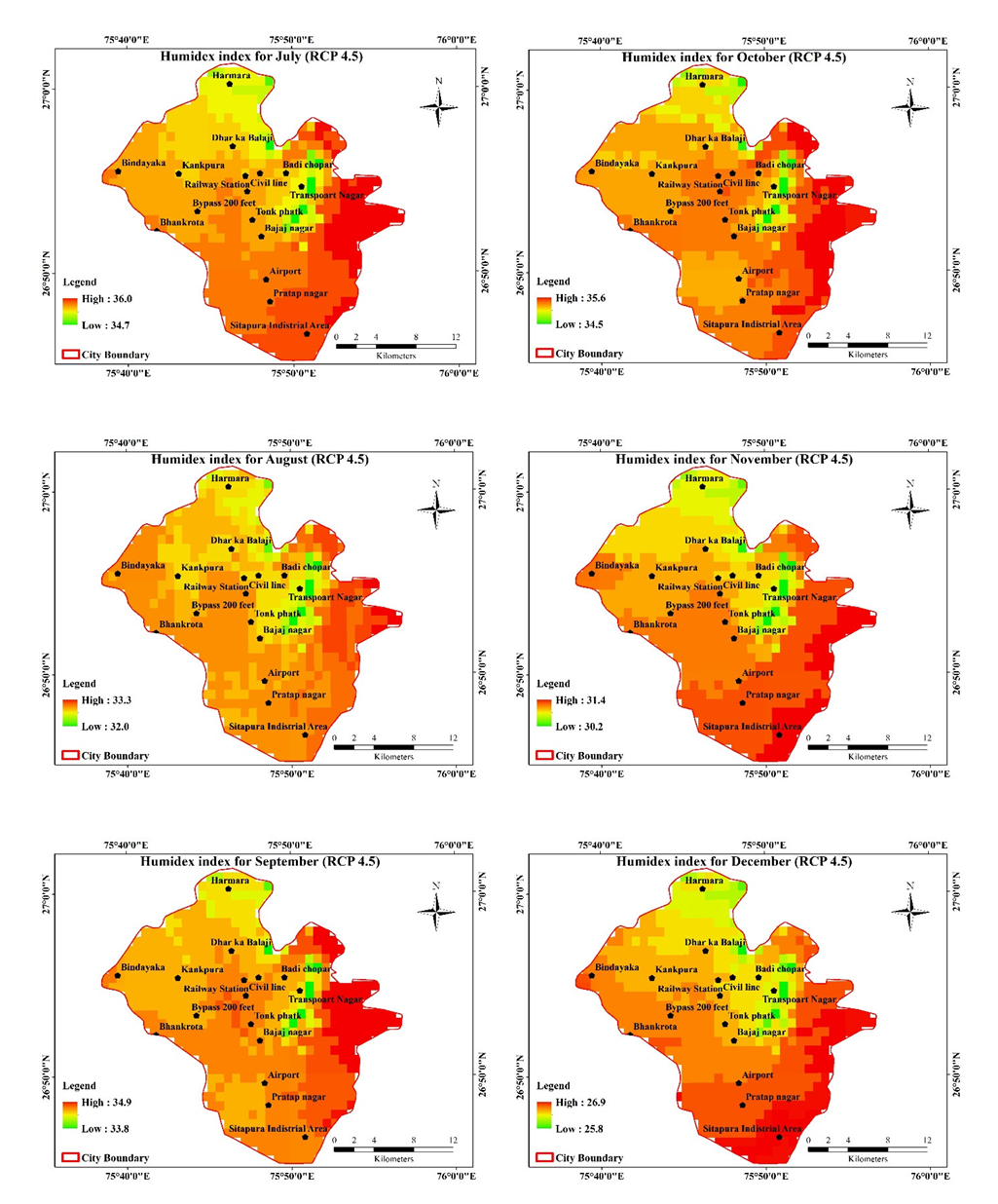
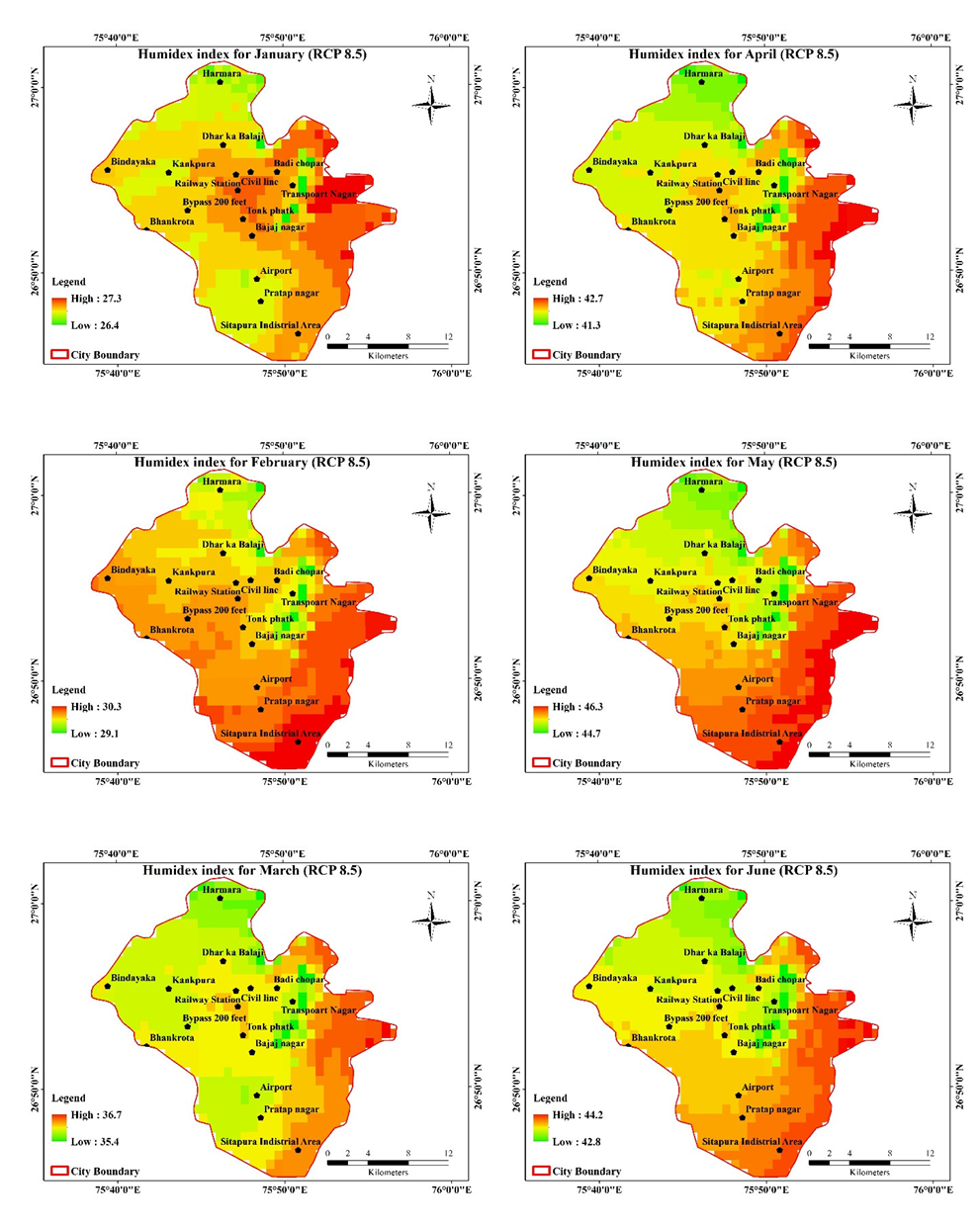
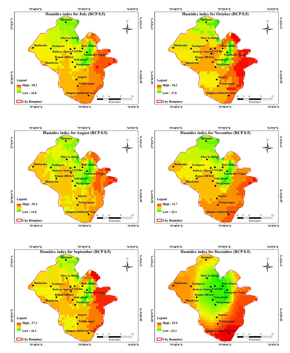
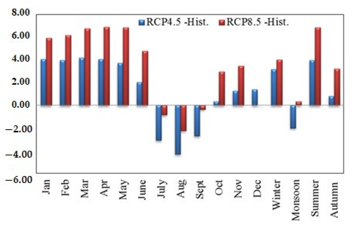
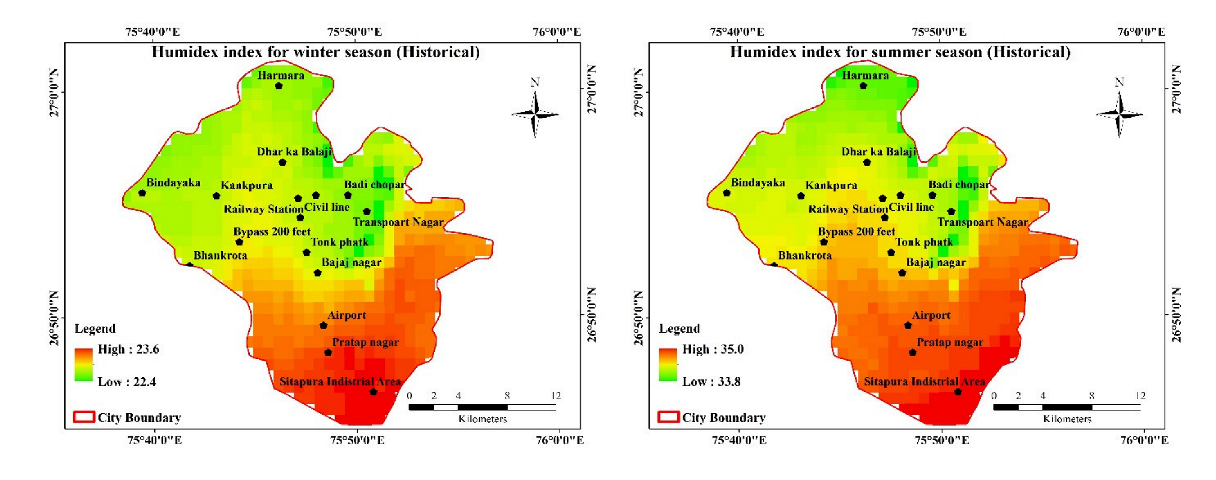
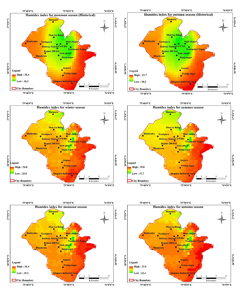
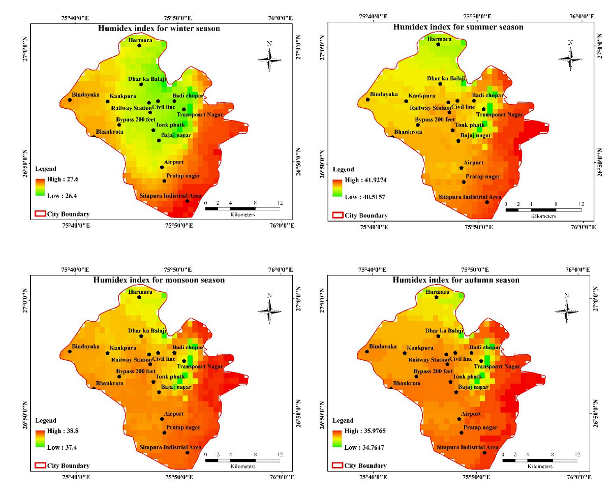
4.2. Humidex Index
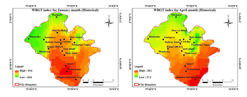
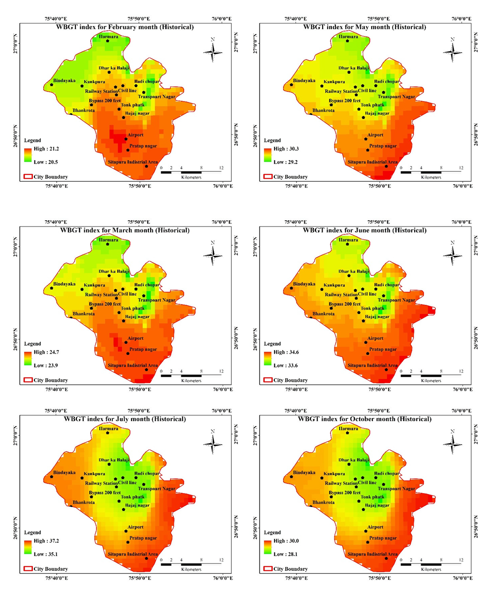
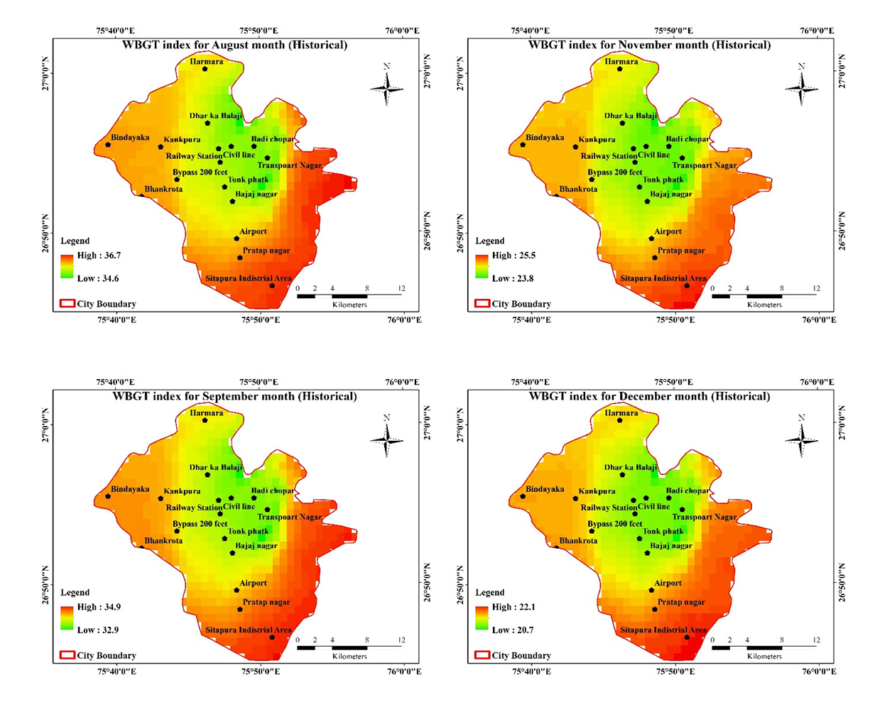
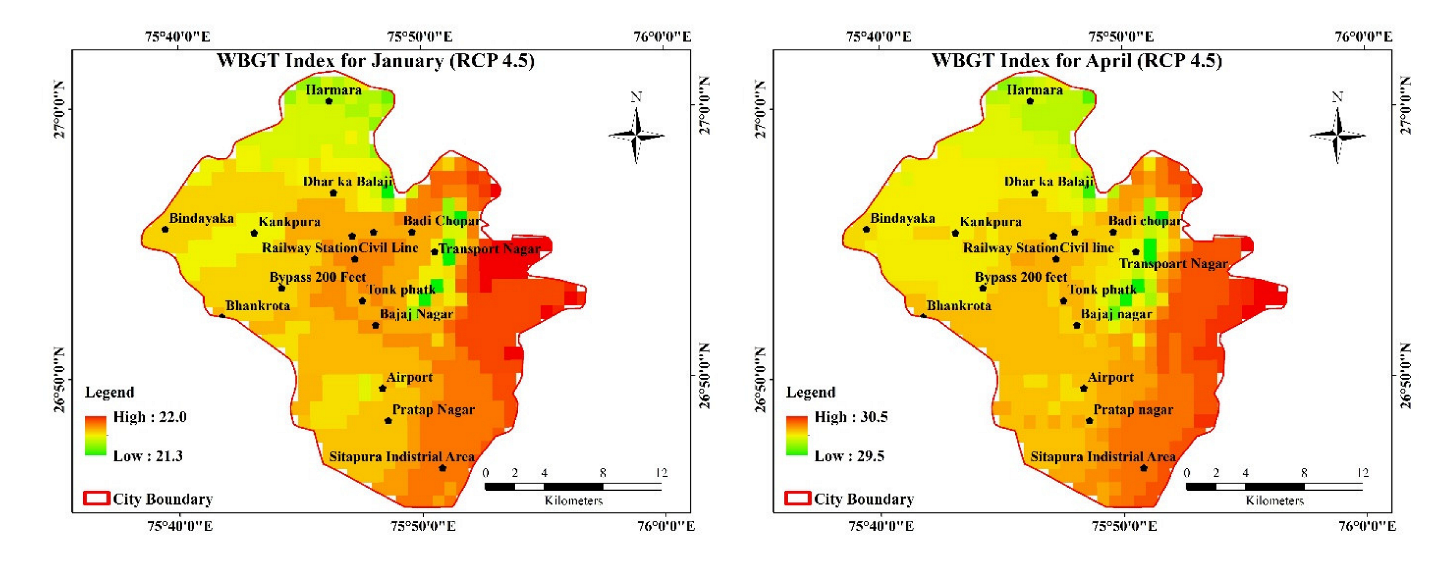
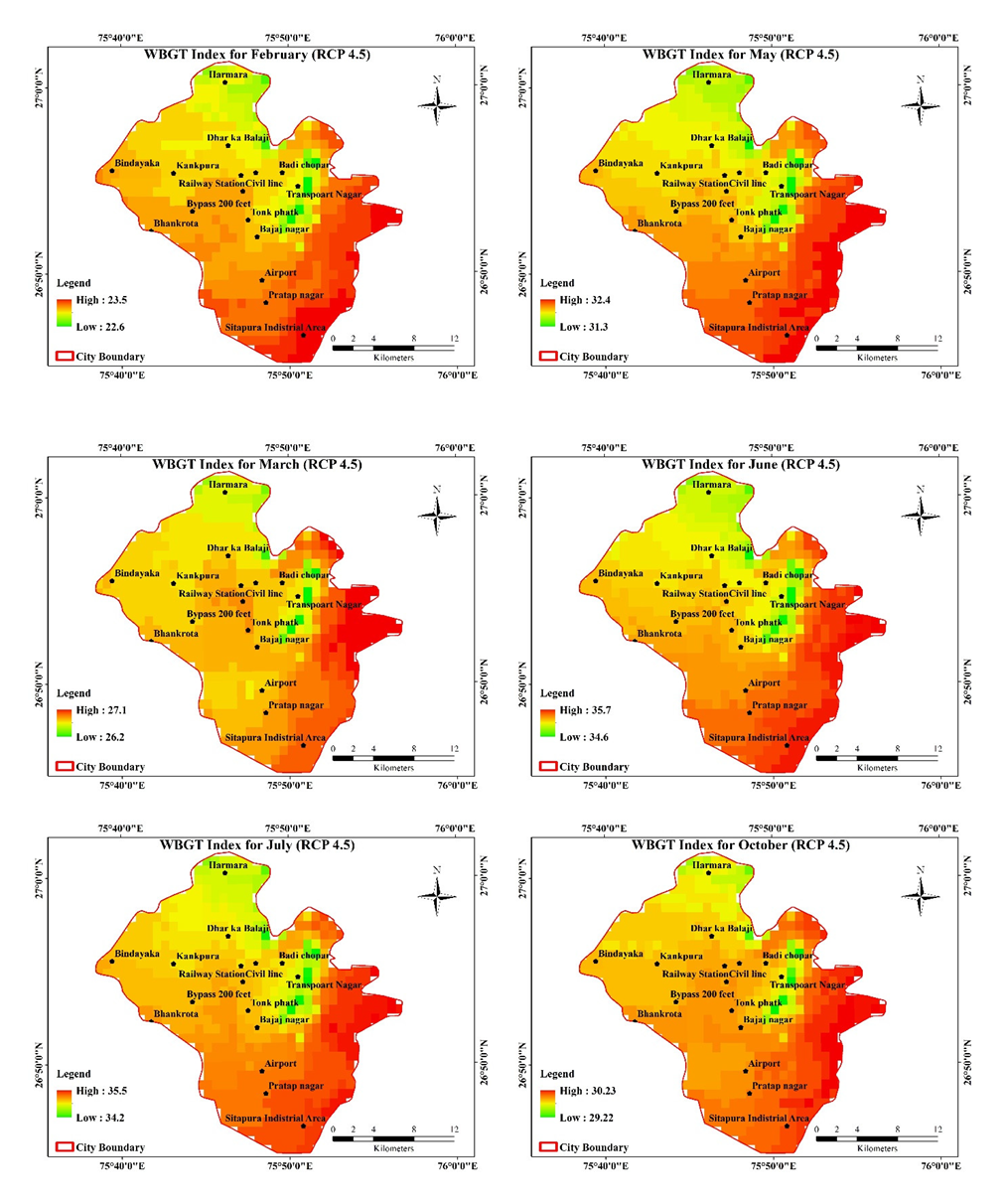
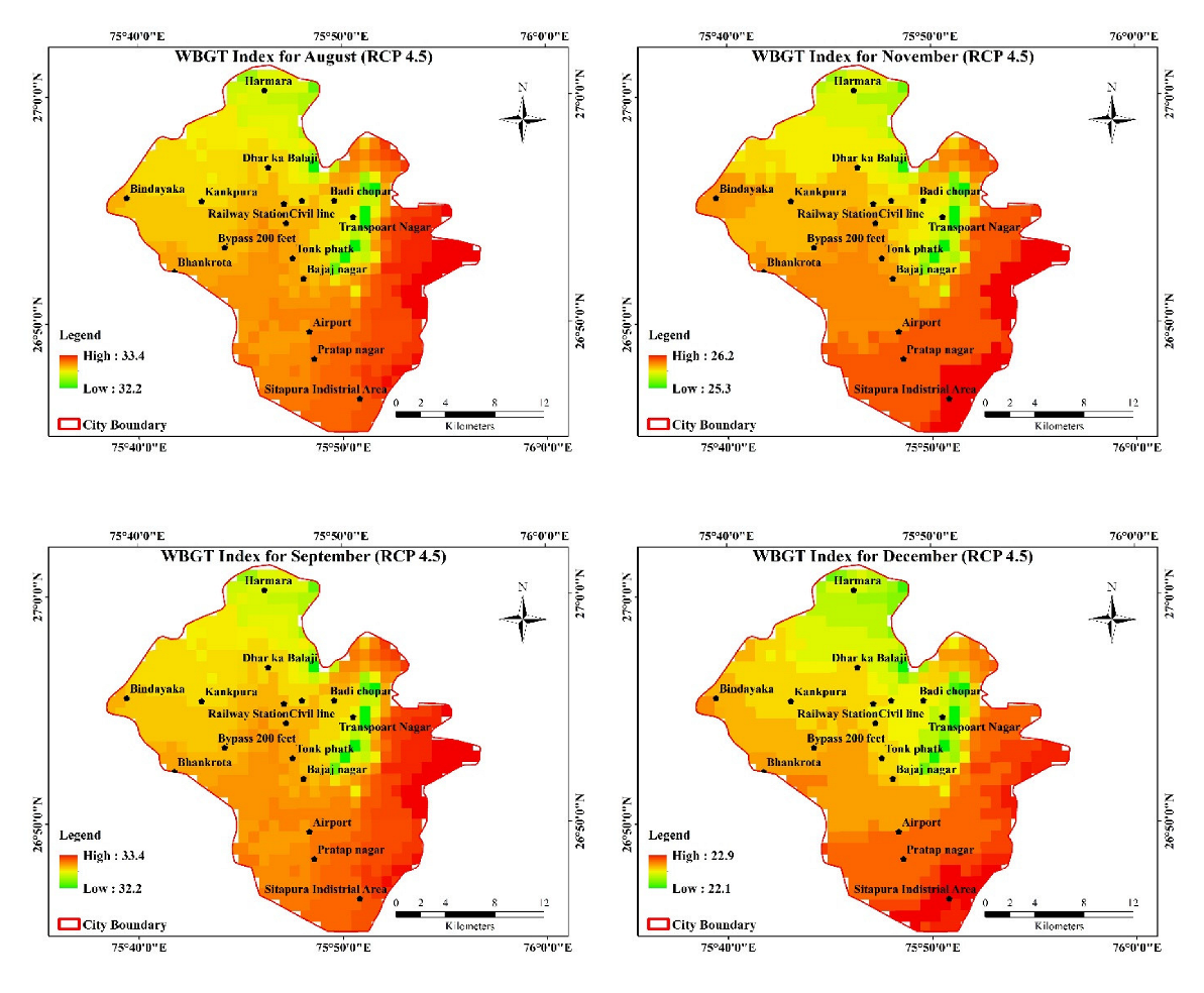
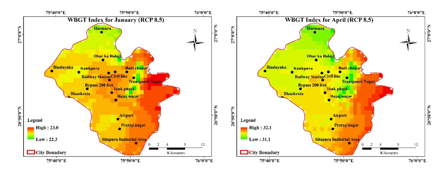
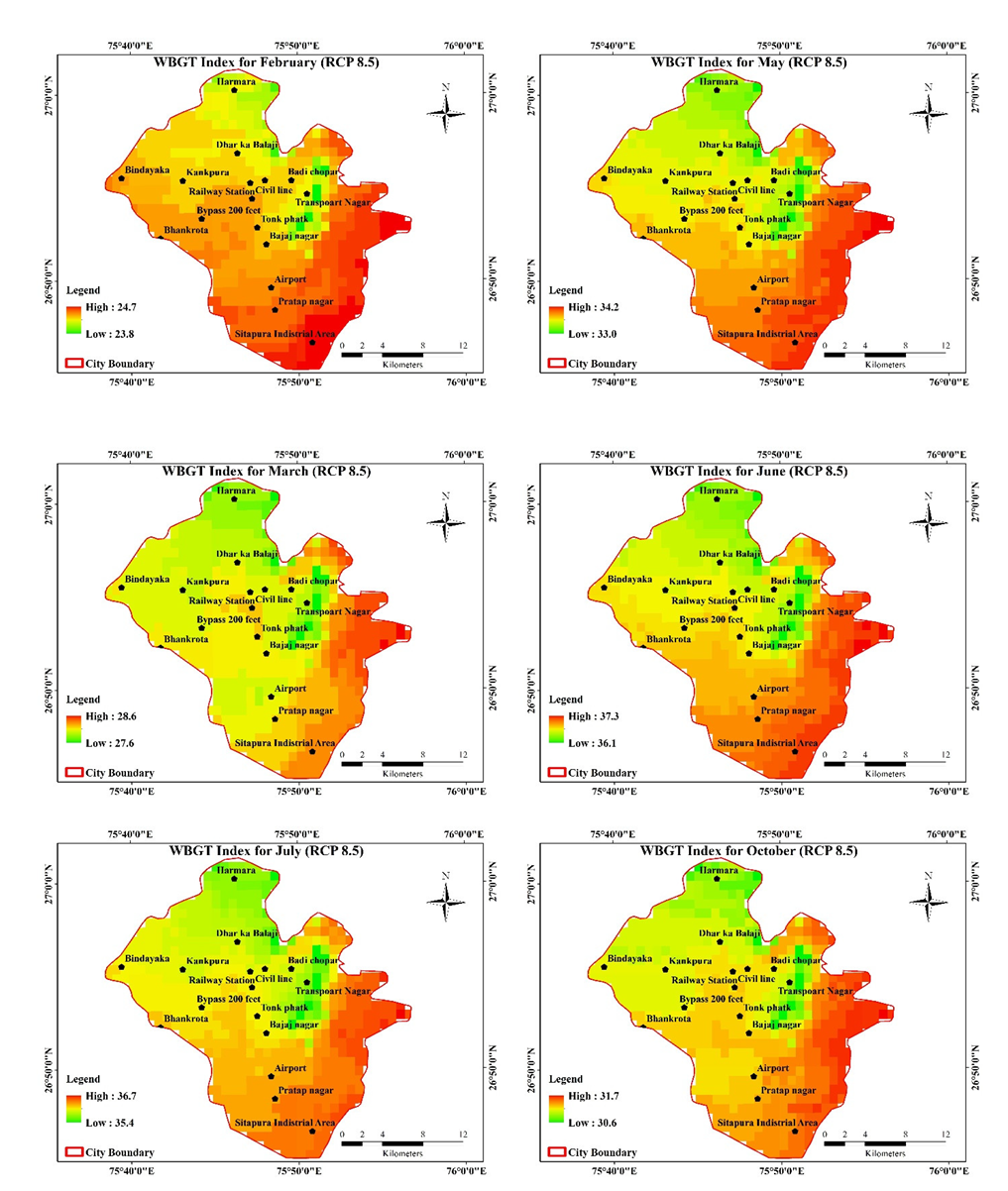
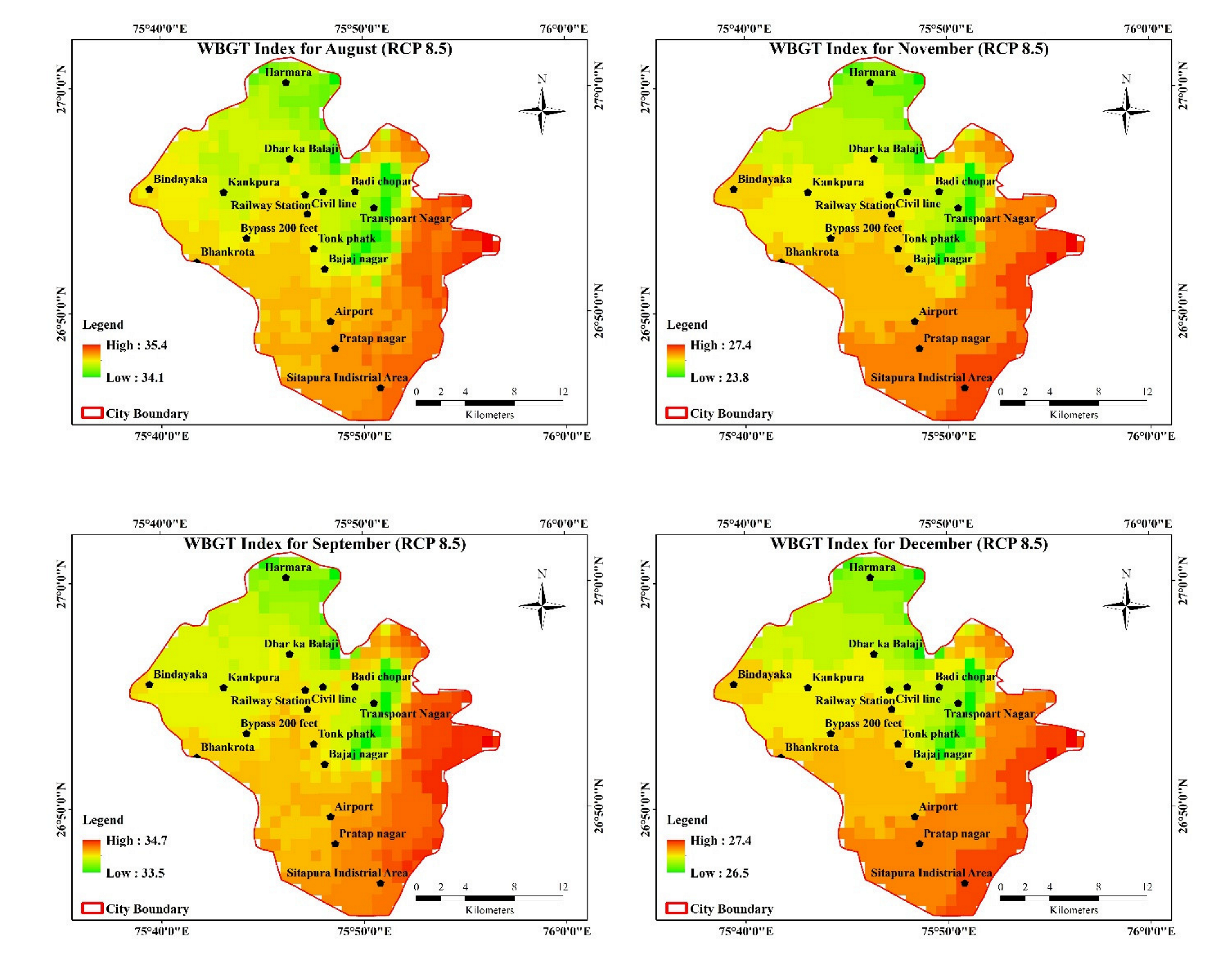
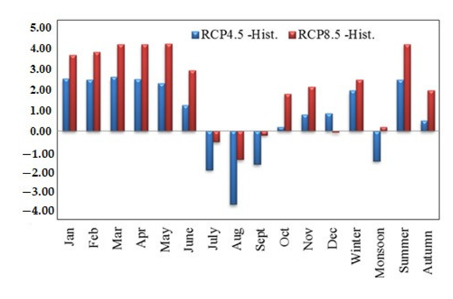
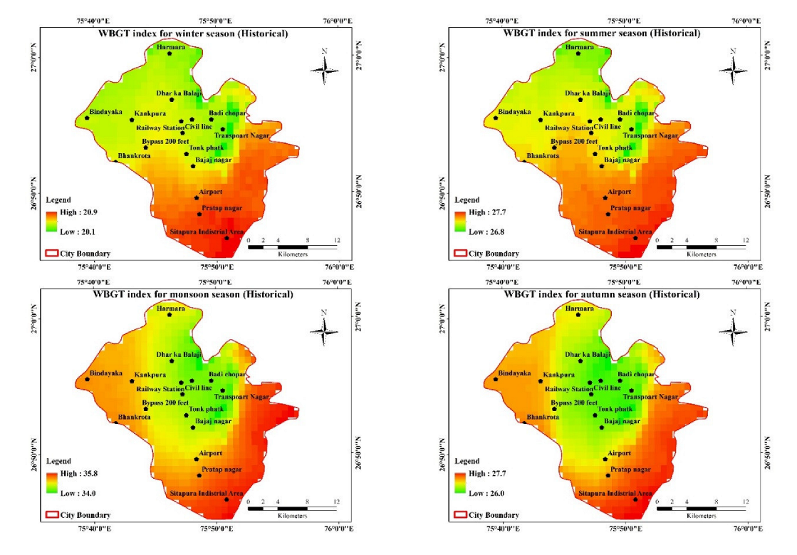
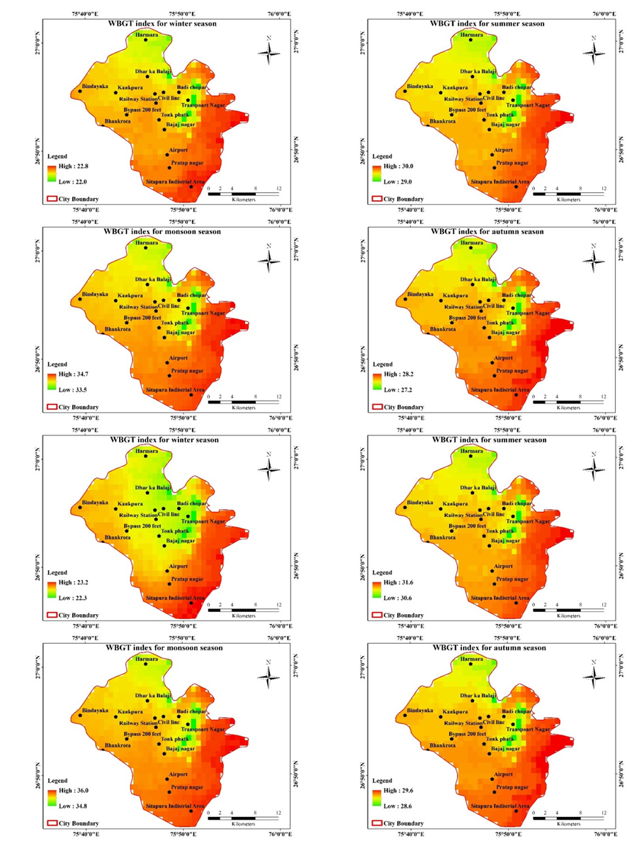
4.3. WBGT Index
4.4. Normalized Difference Vegetation Index (NDVI)
4.5. Soil-Adjusted Vegetation Index (SAVI)
5. Conclusions
Author Contributions
Funding
Institutional Review Board Statement
Informed Consent Statement
Data Availability Statement
Conflicts of Interest
References
- Field, C.B.; Barros, V.; Stocker, T.F.; Dahe, Q. Managing the Risks of Extreme Events and Disasters to Advance Climate Change Adaptation: Special Report of the Intergovernmental Panel on Climate Change; Cambridge University Press: Cambridge, UK, 2012. [Google Scholar]
- Reiner, R.C., Jr.; Smith, D.L.; Gething, P.W. Climate Change, Urbanization and Disease: Summer in the City…. Trans. R. Soc. Trop. Med. Hyg. 2015, 109, 171–172. [Google Scholar] [CrossRef] [PubMed]
- Joon, V.; Jaiswal, V. Impact of Climate Change on Human Health in India: An Overview. Health Popul.-Perspect. Issues 2012, 35, 11–22. [Google Scholar]
- Marland, G.; Boden, T.A.; Andres, R.J. CO2 Emissions. Trends: A Compendium of Data on Global Change; Technical Report; Carbon Dioxide Analisys Center, Oak Ridge National Laboratory: Oak Ridge, TN, USA, 2000. [Google Scholar]
- Rosenzweig, C.; Solecki, W.D.; Hammer, S.A.; Mehrotra, S. Climate Change and Cities: First Assessment Report of the Urban Climate Change Research Network; Cambridge University Press: Cambridge, UK, 2011. [Google Scholar]
- Tan, J.; Zheng, Y.; Tang, X.; Guo, C.; Li, L.; Song, G.; Zhen, X.; Yuan, D.; Kalkstein, A.J.; Li, F.; et al. The Urban Heat Island and Its Impact on Heat Waves and Human Health in Shanghai. Int. J. Biometeorol. 2010, 54, 75–84. [Google Scholar] [CrossRef] [PubMed]
- Dutta, D.; Rahman, A.; Paul, S.K.; Kundu, A. Estimating Urban Growth in Peri-Urban Areas and Its Interrelationships with Built-up Density Using Earth Observation Datasets. Ann. Reg. Sci. 2020, 65, 67–82. [Google Scholar] [CrossRef]
- Gill, S.E.; Handley, J.F.; Ennos, A.R.; Pauleit, S. Adapting Cities for Climate Change: The Role of the Green Infrastructure. Built Environ. 2007, 33, 115–133. [Google Scholar] [CrossRef] [Green Version]
- Kueh, M.T.; Lin, C.Y.; Chuang, Y.J.; Sheng, Y.F.; Chien, Y.Y. Climate Variability of Heat Waves and Their Associated Diurnal Temperature Range Variations in Taiwan. Environ. Res. Lett. 2017, 12, 074017. [Google Scholar] [CrossRef]
- Nag, P.K.; Nag, A.; Sekhar, P.; Pandit, S. Vulnerability to Heat Stress: Scenario in Western India; National Institute of Occupational Health: Ahmedabad, India, 2009. [Google Scholar]
- De, U.S.; Mukhopadhyay, R.K. Severe Heat Wave over the Indian Subcontinent in 1998, in Perspective of Global Climate. Curr. Sci. 1998, 75, 1308–1311. [Google Scholar]
- van Oldenborgh, G.J.; Philip, S.; Kew, S.; van Weele, M.; Uhe, P.; Otto, F.; Singh, R.; Pai, I.; Cullen, H.; AchutaRao, K. Extreme Heat in India and Anthropogenic Climate Change. Nat. Hazards Earth Syst. Sci. 2018, 18, 365–381. [Google Scholar] [CrossRef] [Green Version]
- Mazdiyasni, O.; AghaKouchak, A.; Davis, S.J.; Madadgar, S.; Mehran, A.; Ragno, E.; Sadegh, M.; Sengupta, A.; Ghosh, S.; Dhanya, C.T.; et al. Increasing Probability of Mortality during Indian Heat Waves. Sci. Adv. 2017, 3, e1700066. [Google Scholar] [CrossRef] [Green Version]
- Ghalhari, G.F.; Heidari, H.; Dehghan, S.F.; Asghari, M. Consistency Assessment between Summer Simmer Index and Other Heat Stress Indices (WBGT and Humidex) in Iran’s Climates. Urban Clim. 2022, 43, 101178. [Google Scholar] [CrossRef]
- Mahgoub, A.O.; Gowid, S.; Ghani, S. Global Evaluation of WBGT and SET Indices for Outdoor Environments Using Thermal Imaging and Artificial Neural Networks. Sustain. Cities Soc. 2020, 60, 102182. [Google Scholar] [CrossRef]
- Zare, S.; Shirvan, H.E.; Hemmatjo, R.; Nadri, F.; Jahani, Y.; Jamshidzadeh, K.; Paydar, P. A Comparison of the Correlation between Heat Stress Indices (UTCI, WBGT, WBDT, TSI) and Physiological Parameters of Workers in Iran. Weather Clim. Extrem. 2019, 26, 100213. [Google Scholar] [CrossRef]
- Kakaei, H.; Omidi, F.; Ghasemi, R.; Sabet, M.R.; Golbabaei, F. Changes of WBGT as a Heat Stress Index over the Time: A Systematic Review and Meta-Analysis. Urban Clim. 2019, 27, 284–292. [Google Scholar] [CrossRef]
- Aliabadi, M.; Jahangiri, M.; Arrassi, M.; Jalali, M. Evaluation of Heat Stress Based on WBGT Index and Its Relationship with Physiological Parameter of Sublingual Temperature in Bakeries of Arak City. Occup. Med. 2014, 6, 48–56. [Google Scholar]
- Vatani, J.; Golbabaei, F.; Dehghan, S.F.; Yousefi, A. Applicability of Universal Thermal Climate Index (UTCI) in Occupational Heat Stress Assessment: A Case Study in Brick Industries. Ind. Health 2015, 54, 14–19. [Google Scholar] [CrossRef] [PubMed] [Green Version]
- Gaspar, A.R.; Quintela, D.A. Physical Modelling of Globe and Natural Wet Bulb Temperatures to Predict WBGT Heat Stress Index in Outdoor Environments. Int. J. Biometeorol. 2009, 53, 221–230. [Google Scholar] [CrossRef]
- Willett, K.M.; Sherwood, S. Exceedance of Heat Index Thresholds for 15 Regions under a Warming Climate Using the Wet-Bulb Globe Temperature. Int. J. Climatol. 2012, 32, 161–177. [Google Scholar] [CrossRef]
- Murari, K.K.; Ghosh, S.; Patwardhan, A.; Daly, E.; Salvi, K. Intensification of Future Severe Heat Waves in India and Their Effect on Heat Stress and Mortality. Reg. Environ. Change 2015, 15, 569–579. [Google Scholar] [CrossRef]
- Mathew, A.; Khandelwal, S.; Kaul, N. Investigating Spatio-Temporal Surface Urban Heat Island Growth over Jaipur City Using Geospatial Techniques. Sustain. Cities Soc. 2018, 40, 484–500. [Google Scholar] [CrossRef]
- Chandra, S.; Sharma, D.; Dubey, S.K. Linkage of Urban Expansion and Land Surface Temperature Using Geospatial Techniques for Jaipur City, India. Arab. J. Geosci. 2018, 11, 31. [Google Scholar] [CrossRef]
- Wang, Y.; Gao, J.; Xing, X.; Liu, Y.; Meng, X. Measurement and Evaluation of Indoor Thermal Environment in a Naturally Ventilated Industrial Building with High Temperature Heat Sources. Build. Environ. 2016, 96, 35–45. [Google Scholar] [CrossRef]
- Adekunle, T.O.; Nikolopoulou, M. Winter Performance, Occupants’ Comfort and Cold Stress in Prefabricated Timber Buildings. Build. Environ. 2019, 149, 220–240. [Google Scholar] [CrossRef]
- Masterton, J.M.; Richardson, F.A. Humidex: A Method of Quantifying Human Discomfort Due to Excessive Heat and Humidity; Environment Canada, Atmospheric Environment: Toronto, ON, Canada, 1979. [Google Scholar]
- Foody, G.M. On the Compensation for Chance Agreement in Image Classification Accuracy Assessment, Photogram. Eng. Remote Sens. 1992, 58, 1459–1460. [Google Scholar]
- Ma, Z.; Redmond, R.L. Tau Coefficients for Accuracy Assessment of Classification of Remote Sensing Data. Photogramm. Eng. Remote Sens. 1995, 61, 435–439. [Google Scholar]
- Monserud, R.A.; Leemans, R. Comparing Global Vegetation Maps with the Kappa Statistic. Ecol. Model. 1992, 62, 275–293. [Google Scholar] [CrossRef]
- Batista, G.T.; Shimabukuro, Y.E.; Lawrence, W.T. The Long-Term Monitoring of Vegetation Cover in the Amazonian Region of Northern Brazil Using NOAA-AVHRR Data. Int. J. Remote Sens. 1997, 18, 3195–3210. [Google Scholar] [CrossRef]
- Hajizadeh, R.; Mehri, A.; Jafari, S.; Beheshti, M.; Haghighatjou, H. Feasibility of Esi Index to Assess Heat Stress in Outdoor Jobs. J. Occup. Environ. Health 2016, 2, 18–26. [Google Scholar]
- Golbabaei, F.; Asour, A.A.; Keyvani, S.; Kolahdoozi, M.; Mohammadiyan, M.; Ramandi, F.F. The Limitations of WBGT Index for Application in Industries: A Systematic Review. Int. J. Occup. Hyg. 2021, 13, 365–381. [Google Scholar] [CrossRef]


| GCMs Information | Data Information |
|---|---|
| ACCESS1-0(AC), BCC-CSM1-1(BC), CCSM4(CC), CNRM-CM5(CN), GFDL-CM3(GF), GISS-E2-R(GS), HadGEM2-AO(HD), HadGEM2-CC(HG), HadGEM2-ES(HE), INMCM4(IN), IPSL-CM5A-LR(IP), MIROC-ESM-CHEM(MI), MIROC-ESM(MR), MIROC5(MC), MPI-ESM-LR(MP), MRI-CGCM3(MG), NorESM1-M(NO) | Monthly average maximum temperature (°C*10) GHG Scenarios: RCP4.5; RCP8.5 |
| Heat Stress Category | WBGT Index | Humidex Index | Inferences |
|---|---|---|---|
| Extreme danger | Greater and equal to 40 | Greater and equal to 46 | Dangerous and the risk of heat stroke |
| Danger | 34–39 | 38–45 | Very uncomfortable and avoid physical exertion |
| Extreme caution | 28–33 | 30–37 | Little uncomfortable |
| Caution | 22–27 | 20–29 | Comfortable |
| Users Accuracy % | |||||||
|---|---|---|---|---|---|---|---|
| Year | Water | Vegetation | Urban Settlement | Open Land | Hilly/Rocky Area | Overall Accuracy | Kappa Coefficient |
| 1993 | 100.0 | 95.4 | 96.7 | 97.9 | 69.8 | 0.92 | 0.88 |
| 2010 | 100.0 | 94.7 | 100.0 | 96.6 | 91.2 | 0.97 | 0.95 |
| 2015 | 100.0 | 95.7 | 97.2 | 92.7 | 88.6 | 0.95 | 0.93 |
| Producer Accuracy % | |||||||
| Year | Water | Vegetation | Urban Settlement | Open Land | Hilly/Rocky Area | ||
| 1993 | 100.0 | 98.41 | 87.88 | 90.73 | 91.67 | ||
| 2010 | 100.0 | 97.83 | 98.21 | 95.45 | 100.00 | ||
| 2015 | 100.0 | 94.74 | 99.28 | 86.44 | 93.94 | ||
| Class Name | Area 1993 | Area 2010 | Area 2015 | % Change (2010–1993) | % Change (2015–2010) | % Change (2015–1993) |
|---|---|---|---|---|---|---|
| Water. | 0.4 | 0.9 | 0.8 | 0.10 | −0.01 | 0.09 |
| Vegetation | 84.4 | 88.6 | 45.7 | 0.87 | −9.09 | −8.21 |
| Urban Settlement | 63.9 | 166.5 | 270.5 | 21.75 | 22.03 | 43.78 |
| Open Land | 216.3 | 159.8 | 91.5 | −11.96 | −14.47 | −26.44 |
| Hilly/Rocky Area | 106.9 | 56.1 | 63.4 | −10.76 | 1.55 | −9.21 |
| Historical | RCP4.5 | RCP8.5 | Historical | RCP4.5 | RCP8.5 | |
|---|---|---|---|---|---|---|
| January | 21.4 | 25.5 | 27.3 | C | C | C |
| February | 24.2 | 28.2 | 30.4 | C | C | EC |
| March | 29.9 | 34.1 | 36.7 | EC | EC | EC |
| April | 35.8 | 39.9 | 42.7 | EC | D | D |
| May | 39.5 | 43.2 | 46.4 | D | D | ED |
| June | 39.5 | 41.5 | 44.3 | D | D | D |
| July | 39.1 | 36.0 | 38.2 | D | EC | D |
| August | 37.7 | 33.4 | 35.4 | D | EC | EC |
| September | 37.7 | 35.0 | 37.3 | D | EC | D |
| October | 35.3 | 35.6 | 38.3 | EC | EC | D |
| November | 30.2 | 31.5 | 33.7 | EC | EC | EC |
| December | 25.5 | 26.9 | 25.5 | C | C | EC |
| Winter | 23.7 | 26.9 | 27.7 | C | C | EC |
| Monsoon | 38.5 | 36.5 | 38.8 | D | EC | D |
| Summer | 35.1 | 39.1 | 41.9 | EC | D | D |
| Autumn | 32.8 | 33.6 | 36.0 | EC | EC | EC |
| Historical | RCP4.5 | RCP8.5 | Historical | RCP4.5 | RCP8.5 | |
|---|---|---|---|---|---|---|
| January | 19.7 | 22.0 | 23.1 | C | C | C |
| February | 21.2 | 23.5 | 24.8 | C | C | C |
| March | 24.7 | 27.1 | 28.6 | C | EC | EC |
| April | 28.2 | 30.5 | 32.1 | EC | EC | D |
| May | 30.3 | 32.5 | 34.2 | EC | EC | D |
| June | 34.6 | 35.8 | 37.3 | D | D | D |
| July | 37.3 | 35.5 | 36.8 | D | D | D |
| August | 36.7 | 33.4 | 35.4 | D | D | D |
| September | 34.9 | 33.4 | 34.7 | D | D | D |
| October | 30.0 | 30.2 | 31.7 | EC | EC | EC |
| November | 25.5 | 26.2 | 27.5 | C | C | EC |
| December | 22.2 | 23.0 | 22.1 | C | C | EC |
| Winter | 21.0 | 22.8 | 23.3 | C | C | C |
| Monsoon | 35.9 | 34.5 | 36.1 | D | D | D |
| Summer | 27.7 | 30.0 | 31.6 | EC | EC | EC |
| Autumn | 27.8 | 28.2 | 29.6 | EC | EC | EC |
Publisher’s Note: MDPI stays neutral with regard to jurisdictional claims in published maps and institutional affiliations. |
© 2022 by the authors. Licensee MDPI, Basel, Switzerland. This article is an open access article distributed under the terms and conditions of the Creative Commons Attribution (CC BY) license (https://creativecommons.org/licenses/by/4.0/).
Share and Cite
Chandra, S.; Dubey, S.K.; Sharma, D.; Mitra, B.K.; Dasgupta, R. Investigation of Spatio–Temporal Changes in Land Use and Heat Stress Indices over Jaipur City Using Geospatial Techniques. Sustainability 2022, 14, 9095. https://doi.org/10.3390/su14159095
Chandra S, Dubey SK, Sharma D, Mitra BK, Dasgupta R. Investigation of Spatio–Temporal Changes in Land Use and Heat Stress Indices over Jaipur City Using Geospatial Techniques. Sustainability. 2022; 14(15):9095. https://doi.org/10.3390/su14159095
Chicago/Turabian StyleChandra, Suresh, Swatantra Kumar Dubey, Devesh Sharma, Bijon Kumer Mitra, and Rajarshi Dasgupta. 2022. "Investigation of Spatio–Temporal Changes in Land Use and Heat Stress Indices over Jaipur City Using Geospatial Techniques" Sustainability 14, no. 15: 9095. https://doi.org/10.3390/su14159095