
Soil Erosion Process Simulation and Factor Analysis of Jihe Basin


1
College of Surveying and Geo-Informatics, North China University of Water Resources and Electric Power, Zhengzhou 450046, China
2
Key Laboratory of Soil and Water Conservation on the Loess Plateau of Ministry of Water Resources, Yellow River Institute of Hydraulic Research, Zhengzhou 450003, China
*
Authors to whom correspondence should be addressed.
Sustainability 2022, 14(13), 8114; https://doi.org/10.3390/su14138114
Submission received: 18 May 2022
/
Revised: 28 June 2022
/
Accepted: 28 June 2022
/
Published: 2 July 2022
(This article belongs to the Special Issue Regional Water System and Carbon Emission)
Abstract
:Soil erosion is a notable contributor to carbon emissions. Distributed erosion model can be used to study erosion distribution in different land cover, identify the main influential factors, and hence guide soil and water conservation. In this study, Regional Soil Erosion model (RSEM) was used to simulate the soil erosion processes of Jihe Basin in 2015, and the Multiscale Geographically Weighted Regression (MGWR) implementation was applied to compare the erosion regression of Geographically Weighted Regression (GWR) and MGWR as well as study the impact of influential factors on sediment modulus in hillslopes. The results are as follows: (1) MGWR results indicated slope was the dominant factors affecting soil erosion at the catchment scales, where the average coefficients of slope, forest coverage, and grass coverage descended in the value of 0.90, −0.11, and −0.19, and the influences of factors operate over scales; (2) MGWR with the adoptive bandwidths performed well in the goodness of fit, t-test of variables, scales that variables operate, and interactive interpretation of soil erosion; (3) the coupling effects and scales of vegetation and topography factors are an important approach to study soil erosion at a larger scale.
1. Introduction
Soil is the third largest global carbon stock except for ocean and lithosphere, and an important contributor to greenhouse-gas emissions in the terrestrial ecosystem [1,2]. Soil erosion is a widespread and notable environmental problem threatening the terrestrial ecosystems [3], relevant to non-point pollution [4], land degradation [5], carbon cycle, etc. Considerable quantities of topsoil are transferred by soil erosion, greatly affecting carbon redistribution and global biochemistry [6]. The Loess Plateau is one of the most intensely eroded areas in the world, and its dry climate and rare vegetation are the primary factors of the extremely fragile eco-environment [7]. Serious soil erosion not only aggravates the deterioration of the local ecology, but also is the cause of considerable carbon flowing into the global eco-environment [8]. With the effective implementation of the Grain-for-green project, the eco-environment of the Loess Plateau has changed significantly that the average annual amount of sediment entering the Loess Plateau has been drastically reduced from 1.6 billion ton to 0.3 billion ton [9], regulating regional climate, fixing carbon, sustaining water balance, and increasing biodiversity [10,11]. Previous studies indicated vegetation restoration on a large scale has been the key reason for the reduction of sand transport in major river basins, especially the Yellow River basin in the past 30 years [12,13,14]. However, the capacity vegetation restoration reduces soil erosion and carbon emission is unclear and hence quantifying the volume of erosion reduction at the watershed scale is urgent [15].
Soil erosion by water is a multifactorial coupled influence process, affected by precipitation [16], topography [17], soil [18], and vegetation [19]. The relationship between single factor and erosion of sediment production has been well established. Vegetation cover and topography play an important role in the soil erosion and sediment transportation by modifying characteristics of runoff and erosion dynamic; for example, canopy of tree and vegetation can intercept rainfall and reduce the kinetic energy of rainfall, thus slowing down surface erosion by splashing; the root layer of vegetation can improve the physical and chemical properties of the soil, enhance its infiltration and erosion resistance, and ultimately prevent soil from erosion; the vegetation surface cover part, especially the deadfall layer, can directly absorb and retain rainfall, and increase soil infiltration and reduce surface runoff by reducing runoff flow rate and extending sink time [20,21,22]. Topography is the vehicle through which erosion of sand production occurs and develops. Under certain rainfall conditions, slope is the main topographic indicator that determines erosion and sand production. However, the response mechanism of erosion and sediment yield under the coupling effect of multiple factors is unclear [20]. Particularly, the function of vegetation and topography in watershed-scale is still weak.
Soil erosion model is an effective tool for predicting soil erosion, guiding the configuration of soil and water conservation measures, and optimizing the use of soil and water resources, which have long been of great interest to scholars in the world [23]. Numerous models have their typical characteristics in terms of scenarios, description of the erosion process and accuracy, such as RUSLE (Revised Universal Soil Loss Equation), WEEP (Water Erosion Prediction Project), PESERA (Pan-European Soil Erosion Risk Assessment), SWAT (Soil Water Assessment Tool), LISEM model (LImburg Soil Erosion Model), EUROSEM (European Soil Erosion Model), etc. Previous studies showed that the erosion model has been used to quantitatively simulate and assess regional soil loss [24]. RUSLE is the most popular model capable of predicting the average annual soil loss because of its convenience in application and compatibility with GIS [25]. WEEP is a process-based model used to predict runoff and soil erosion and can be applied to slopes and small catchments due to single rainfall-event simulation [26,27]. PESERA assesses the state of soil erosion risk on a European scale and can be used to assess sensitivity to altered conditions, especially in the prediction of post-fire erosion loss [28,29]. Generally, soil erosion models can be divided into statistical models and theoretical models. Statistical models have advantages in effective assessment of soil loss, but they lack detailed descriptions of erosion processes and poorly explain the influencing factors on erosion [30]. Physical models, especially distributed physical genesis models, are more suitable for fine-grained assessment of erosion processes and sand transport processes, whereas the data required for modeling are difficult to obtain which makes it difficult to determine and apply model parameters in varied areas [31]. Considering the regional availability of erosion model and data availability of input parameter, this study applied a distributed physical genesis models with flexible input termed Regional soil erosion model (RSEM) to simulate the soil erosion process of Jihe Basin. Based on the principles of hydrology and erosion, RSEM quantitatively describes the process of soil erosion in a watershed from the perspective of precipitation and sediment generation and transportation, including precipitation, vegetation interception, soil infiltration, storage in micro depressions, surface runoff, sediment detachment and deposition, and sediment accumulation and transmission [32].
Regression analysis describes how one or more independent variables contribute to the dependent variable, which could demonstrate the relationship in numeric variables. Non-independent spatial data will lead to the inapplicability of many classical statistical methods that are independently and identically distributed [33]. Obviously, soil erosion at the watershed scale is spatially heterogeneous. Ordinary Least Squares (OLS) is a common mathematical regression analysis method, which minimizes the residual sum of squares to the analysis of the relationship in different variables. While the spatial distribution of variables is heterogeneous and non-stationarity, OLS is difficult quantify the correlation of spatial variable. Geographically weighted regression (GWR) has been one of the wide-used local spatial statistical analysis, calibrating locally weighted regression analysis models where parameter estimations vary with its location, providing intuitive, practical spatial relationship heterogeneity, and multiphase analysis tool [34]. GWR typically provides increased model fit and reduced residual spatial autocorrelation compared to a traditional global regression [35]. To capture the process of spatial heterogeneity by allowing effects to vary over space, GWR uses nearby data to calibrate an ensemble of local linear models and provides a surface of location-specific parameter estimates for each relationship in the model that is allowed to vary spatially with a fixed bandwidth parameter [36]. The issue of scale is one of the important research elements of geographic information science [37]. While calibrating the GWR model with a single bandwidth and kernel function, it is inevitable to lead to the spatial variation of all parameter estimates showing the same scale characteristics. Though the multivariate spatial data relationships correspond to different scales of variation, GWR reflects the ‘best average’ scale of spatial relationships for all and ignores these differences and reflects the spatial relationships at the differences. To fix the scale issue, Fortheringham proposed the Multiscale Geographically Weighted Regression (MGWR) representing the spatial heterogeneity of multivariate estimation with adoptive bandwidths in 2017 [38]. Then Yu complemented the inferential statistics so that MGWR is widely applied in varied research [39]. Few studies use MGWR to analyze multiple factors related to erosion.
Jihe basin, the first-class tributary of the Wei River in the Loess Plateau, has considerable reduction of sediment transport volume in the past forty years, from 10.4 billion Kg in 1968 to 0.18 billion Kg in 2008 [40]. After years of efforts of soil and water conservation projects, the ecosystem and soil erosion in Jihe basin have accumulated a wealth of observation data needed to further study. However, previous studies mostly focused on the statistical analysis how land cover contributes to sediment reduction at the sub-basin level of Jihe basin [41,42,43].
This study applied RSEM to simulate the soil erosion process of Jihe Basin in 2015 and MGWR software, developed by Oshan, to explore the spatial impact on erosion of topography and vegetation from the perspective of the hillslopes scale. The purpose of this study was to: (1) simulate the process of runoff generation, soil erosion and sediment yield in Jihe Basin; (2) apply MGWR to demonstrate the influential factors to spatial distribution of erosion; (3) explore how vegetation and topography factors impact on erosion at the watershed scale.
2. Materials and Methods
2.1. Study Area
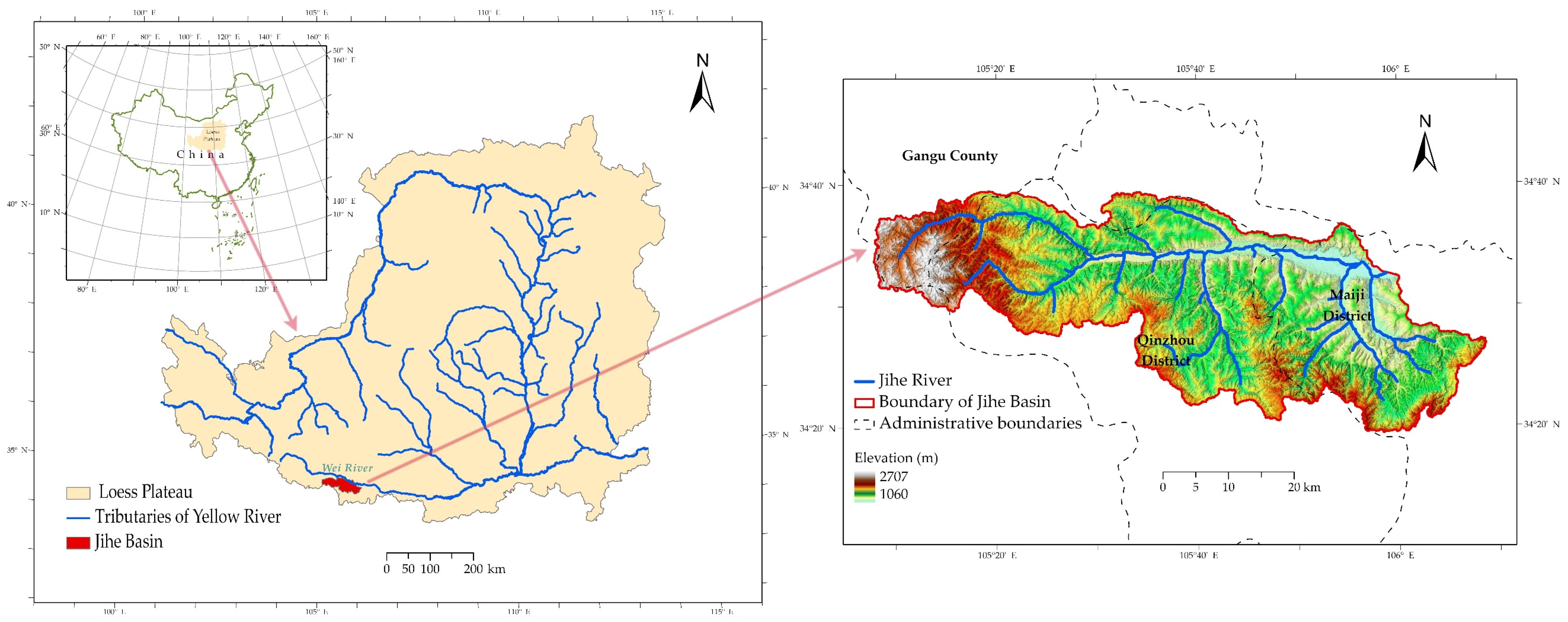
As shown in Figure 1, Jihe basin is the first-class tributary of the Wei River that locates in the southeast of the Loess plateau and belongs to the third sub-region of Loess hills. Originating in Gangu County, Jihe basin flows eastward through Qinzhou District and joins the Wei River in Maiji District, which covers about 1800 Km2 at 105°8′ E–106°8′ E in longitude and 34°21′ N to 34°39′ N in latitude. The topographic features of the basin are mainly loess hills, laterite hills, erosion landforms of earth and stone hills and river valley terraces [41]. According to the Harmonized World Soil Database constructed by Food and Agriculture Organization of the United Nations, soil type in Jihe basin varies greatly, in which 37.92% is cinnamon soil, 23.36% is loessial soil, 16.00% is brown soil, 15.59% is alluvial soils, 5.48% is skeleton soil, and 1.84% is mountain meadow soil. The watershed is a warm temperate semi-humid and semi-arid transition zone.
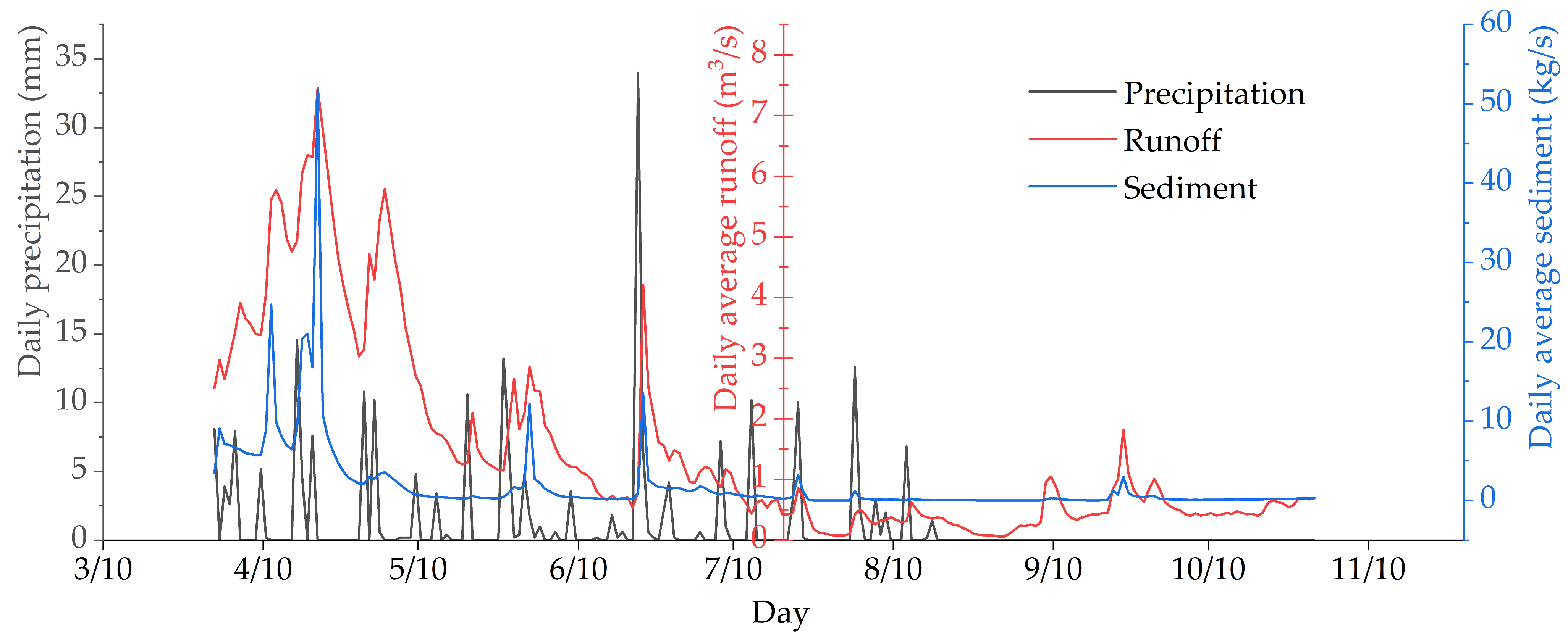
According to Tianshui hydrological observatory data collected in Hydrological Data of Yellow River Basin of Annual Hydrological Report, its average annual precipitation is about 566.8 mm from 1976 to 2015, and the minimum precipitation is 368 mm in 1996 and the maximum is 860 mm in 2003. With an unevenly distributed precipitation, it concentrates on summer that over 60% of precipitation occurs in the way of fast and strong rainstorm from June to September [40]. The rainfall events in summer of 2015 were used to study soil erosion of Jihe Basin. Figure 2 showed the curve of precipitation, runoff, and sediment yield in 2015, in which there were two important rainfall events worth to further analyze. According to observation data of hydrological yearbook, the precipitation volume of two rainfall occurred in April and June was 211.5 mm and accounted for 53.97% in 2015, followed by 2.39 × 10⁷ m3 of runoff and 3.46 × 10⁷ Kg of sediment which accounted for 67.88% and 95.61%, respectively. In Figure 2, the curve lines showed a simultaneous trend of precipitation, runoff, and sediment yield, and indicated sediment by soil erosion was mainly generated by intensive rainfall and runoff. Therefore, two heavy rainfalls in April and June were applied in model to simulate soil erosion.
2.2. RSEM Model Simulation
2.2.1. The Framework of RSEM
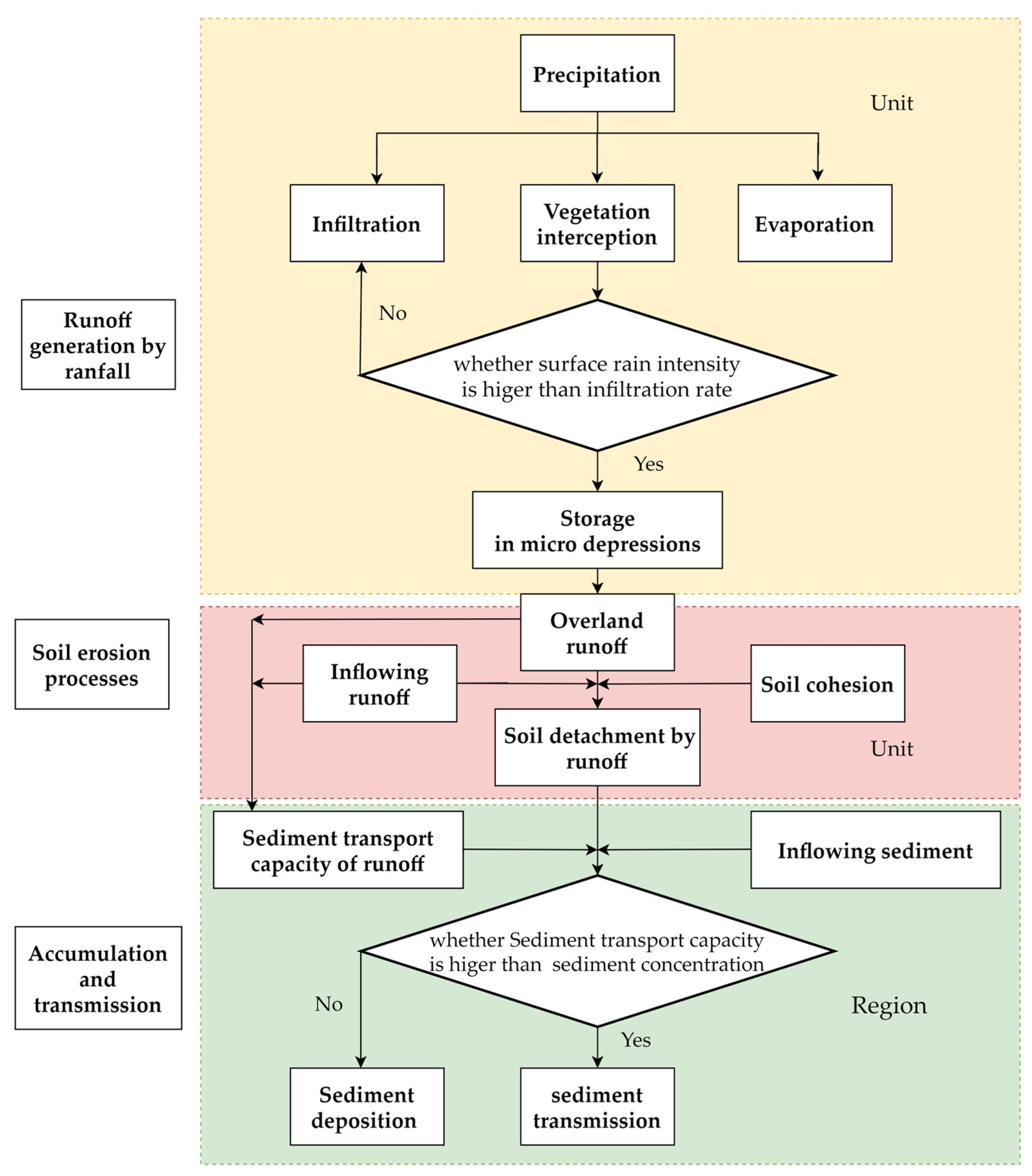
The Regional soil erosion model (RSEM) quantitatively simulates the surface material transport processes by describing the soil erosion process at the catchment scale as rainfall and runoff generation, soil erosion, runoff, and sediment transportation. As shown in Figure 3, the processes of soil erosion in this model are divided into three parts at the hydrological unit scale, including runoff generation by rainfall, sediment yield by runoff, and accumulation and transmission of runoff and sediment. The sub-processes of interception [44,45] (Equations (1) and (2)), infiltration [46] (Equation (3)), storage in micro depressions [47] (Equation (4)), transport capacity [48] (Equation (5)), detachment and deposition [49] (Equation (6)) are listed as follows. Two key equations (Equations (5) and (6)) that determine the calculation of detachment volumes could also be found in LISEM model (LImburg Soil Erosion Model) [50] and EUROSEM (European Soil Erosion Model) [51]. A more detailed mechanism and implementation process are described in the paper [32,52].
where is the cumulative interception (mm), is the cumulative rainfall (mm), η is a correction factor for vegetation density and determines the rate with which is reached, is the fraction of vegetation cover and is the canopy storage capacity (mm) estimated from the LAI (m2/m2), calculated in Equation (2).
Infiltration can be calculated with Equation (3).
where is infiltration rate (mm/min); is infiltration rate at steady state (mm/min); is time since the start of the infiltration (min); and is coefficients relating to soil character and original condition.
where is maximum depression storage (cm); is random roughness (cm); is slope gradient (%).
where is transport capacity (kg·m−3); is flow velocity (m/s); is slope (%); and are experimental coefficients depending on the median texture (D50) of the material.
where is detachment volume of runoff (kg/s); is effective coefficient of runoff detachment; and are the image resolution (m); is sediment particle deposition rate(m/s); is transport capacity (kg·m−3) and is the sediment concentration(kg·m−3).
According to the principle of water-sand balance and the support of GIS, the algorithms on accumulation and transmission of runoff and sediment was designed under the principles of accumulation and GIS spatial analysis [52], which can calculate the runoff and sediment yield on outlet of basin.
2.2.2. Input and Output of RSEM
Input of RSEM includes precipitation, DEM (Digital Elevation Model), and land cover. Daily precipitation in 2015 was provided by Tianshui hydrological observatory. The precipitation data including precipitation volumes and rainfall duration in April and June was used to simulate the rainfall processes, which were indicators of rainfall erosivity. Since the sediment volumes yielded by the precipitation rainfalls in April and June contributed to 95.61% of sediment volumes of 2015, this study mainly focuses on sediment yield by soil erosion, and hence other time series were ignored because of low sediment yield. The DEM dataset of STRM (Shuttle Radar Topography Mission)) and Landsat image in this study was collected and derived from Geospatial Data Cloud (http://www.gscloud.cn/, accessed on 15 July 2015). Slope were calculated from DEM. The LUCC of catchment was interpreted into five categories from Landsat image, combined artificial interpretation with random-forest algorithm. Both the former with a resolution of 25 m and the latter with a resolution of 30 were resampled to the resolution of 75 m with the nearest neighbor method. LAI calculated from Landsat image was to calculate the cumulative vegetation retention [53]. Combined the Kostiakov infiltration model with the measured data from field infiltration process experiment, the coefficient of Kostiakov model was interpolated to a region surface to calculate infiltration.
The output of model is presented as raster image which could be used to further analyze and verify model. The key simulation results include, sediment transport capacity, sediment transport volume on outlet of basin, soil detachment by runoff, sediment modulus, etc.
2.2.3. Validation of Simulation Results
The validation of simulation results of RSEM were verified by the measured data of Tianshui hydrological observatory, including volumes of sediment transport collected in Hydrological Data of Yellow River Basin of Annual Hydrological Report. The volumes of sediment transport were calculated from a daily average rate of suspended sediment transport (Kg/s) during the corresponding period. Since the catchment area that Tianshui hydrological observatory covers is about 1019 Km2 in hydrological yearbook of Jihe basin while the study area that is similar in soil characteristics and topography covers about 1800 km2 [54], the measured volumes of sediment were adjusted to multiply the factor (1.8), so that the simulation results could be verified by the measured date. The simulated sediment volumes of basin outlet in April and June were validated in the comparison with the adjusted measured sediment volumes.
2.3. Data Analysis
Since the calculation of runoff and sediment volumes include the processed of accumulation and transmission in units, each unit are the sum of the retained volume of the last iteration, runoff by precipitation/detachment by the runoff, inflow, and outflow of runoff/sediment by the accumulation function of Arcgis. Therefore, each unit is not isolated during the calculation and not merely determined by equations above. It is meaningful and scientific to render analysis about the correlation between sediment modulus and influential factors at the hillslope scale.
The soil erosion simulation results by the rainstorm in April of 2015 were used to participate in the further study since it was the largest soil erosion event in 2015. OLS, GWR, and MGWR regression model were used to participate in regression among sediment modulus, vegetation, and topography. Sediment modulus was used to describe soil erodibility of hillslopes which means the amount of erosion per unit area during a rainfall event. Forest coverage and grass coverage was used to be an indicator of vegetation factor and average slope was to be an indicator of topography. After the simulation of soil erosion, the values of sediment modulus stored in the pixel of raster image were calculated at each hillslope extracted by the hydrological function of Arcgis. Vegetation coverage and average slope participated in regression analysis at the hillslopes were calculated by Python.
MGWR implementation, developed by Oshan, is a multiscale analysis tool of spatial heterogeneity, providing novel functionality for inference and exploratory analysis of local spatial processes, new diagnostics unique to multi-scale local models, and drastic improvements to efficiency in estimation routines, including OLS, GWR, and MGWR regression models [36].
By borrowing data nearby to distance-weight at each location, GWR calibrates a separate regression model allowing the parameters to vary spatially. The GWR model formulation can be specified as Equation (7):
where is the th predictor variable, is the th coefficient, is the error term, and is the response variable.
MGWR eliminates the restriction that all relationships vary at the same spatial scale so that the conditional relationships between the response variable and the different predictor variables are allowed to vary at different spatial scales [55]. The MGWR model formulation can be described as Equation (8):
where in indicates the bandwidth used for calibration of the th conditional relationship.
Two key issues in both GWR and MGWR model calibration are kernel function and optimized bandwidth selection. Kernel function and bandwidth selection are used to calculate the weights matrix of both GWR and MGWR models. In this study, adaptive bis-square kernel was selected as spatial kernel and Corrected Akaike information criterion (AICc) was selected as the optimization criterion to select the optimized bandwidth. AICc penalizes smaller bandwidths that result in more complex models that consume more degrees of freedom and is defined as Equation (9). AICc weights the complexity of the estimated model and the goodness of model to fit the data and the lower AICc means better fitness. When AICc values change more than 3, one model is significantly different from the other [36]. The dependent and independent variables were standardized so that they are centered at zero and based on the same range of variation which makes calculation quicker, the and parameter estimation can be easily reversed so that the regression equation demonstrates the origin of quantitative relationships.
where n is the number of observations, S is the influence or hat matrix, and RSS is the residual sum of squares.
According to the first law of geography, the basic guidelines GWR used to the weights matrix is that the greater the distance, the higher the weight value assigned [56]. Three most widely used kernel functions are provided in MGWR implementation, which are the Gaussian, exponential, and bi-square kernel. The bi-square kernel makes observations beyond the bandwidth non-influential while the other two kernels make all observations to retain non-zero weight. The difference between fixed and adoptive kernel function is whether the bandwidth parameter is fixed or not. Adaptive kernel has advantages when handling irregularly shaped study areas, non-uniform spatial distributions of observations, and edge effects.
After regression model calibration, several statistics can be used to evaluate the fit of the model. There are global statistics such as residual sum of squares, the adjusted R2 or AICc to assess goodness of fit globally, and the map of local R2 to assess the fit of the model at each location by providing an indication of how well the model fits over the study area. Traditional inferential tools are available, and hence the t-test could be carried out on individual parameter estimation at each location. Effective number of parameters are the measure of model complexity and represent the equivalent number of independent parameters estimated in a local model, which equal the sum of the covariate-specific effective number of parameters [39].
3. Results
3.1. Vegetatio and Topography in Jihe Basin
Slope image, land cover image, and hillslope image were loaded as numpy array by Rasterio python package and summed in the form of average slope and land cover in each hillslope by Numpy python package. Next, slope and vegetation (include forest and grass) in hillslopes were divided into several grades and aggregated by areas, shown in Table 1 in detail. The hillslopes with the average slope of 15–20° accounted for the largest proportion in catchment, and the second is the hillslopes with slope of 20–25°. The steep hillslopes over 15° was dominant landform because of its areas of 1455.38 Km2 and percentage of 81.18%. Similarly, the hillslopes with the vegetation coverage of 70–100% accounted for the largest proportion which was 759.54 Km2 and 42.36% in Jihe Basin, which indicated there was fine vegetation cover in Jihe Basin. Indeed, hillslopes with high vegetation coverage over 50% were concentrated in steep slope over 15°, which is 1308.09 Km2 and about 73% of the total areas in Jihe Basin and meant there were spatial correlation among them and could be further verified.
3.2. Model Simulation Results
Simulation results of sediment was aggregated in Table 2, which showed the volumes of simulated sediment were in the same magnitude compared to the adjusted sediment. Although precipitation in April was lower than that in June, the volumes of sediment in April were higher than that in June, which could be explained by rainfall erosivity. Rainfall erosivity is related to rainfall intensity, including duration of rainfall and precipitation volumes [57]. According to calculation equation of rainfall erosivity [57], higher rainfall erosivity in April may account for the higher sediment volumes, shown in the sharp precipitation curve of Figure 2.
Sediment modulus of simulation result in April were aggregated in hillslopes of varied vegetation coverage and slope degree in Table 3. Since there was null of the areas in Table 1, there was same null data in Table 3. The average of sediment modulus increased significantly with the increase of average slope in hillslopes in which the min was 24,587 Kg/Km2·a and the max was 53,297 Kg/Km2·a. It showed the similar increase with the increase of vegetation coverage in hillslopes. Besides, Table 3 indicated that the sediment modulus varied indistinctively under certain slope degrees and different vegetation coverage and varied significantly under certain vegetation coverage and different slope degrees. This controversial increase with vegetation coverage would be explained later.
3.3. Regression Model Results
Vegetation and topography factors of hillslopes extracted from simulation results was applied in MGWR implementation to study the spatial relationship of sediment modulus at the catchment scale, shown in Table 4, Table 5 and Table 6.
Compared with fitting performance, and the t-test of variables in Table 4 and Table 5, MGWR performed well in three liner models. The fit of goodness descended in the order of GWR, MGWR, and OLS, with adjust-R2 being 0.93, 0.92, and 0.87 respectively. The results of AICc presented a similar order and values of AICc changed more than 3, which indicated there were significant differences in three models. The result of residual sum of squares was opposite order, with the highest value being OLS and the lowest value being GWR. The effective number of parameters were 349.69 for GWR and 223.20 for MGWR, which indicated that MGWR had less complexity and less independent parameters estimated in a local mode compared to GWR. On the other hand, the t-test of variables in three models revealed a complicated result, shown in Table 5. In the OLS model, the t-test of forest coverage and average slope were significant while grass coverage was non-significant, where p = 0.05. In GWR and MGWR model, the t-test of variables in each hillslope was independent, and hence it would be partially significant and partially non-significant. In the GWR model, forest and grass coverage were non-significant while the average was partially non-significant, where p = 0.05. In MGWR model, both three variables were significant, where p = 0.05. Therefore, the t-test results of OLS and GWR revealed there were non-significant across variables because of non-independent spatial data that are not independently and identically distributed [33]. Based on the comprehensive indicators of fitness above, MGWR performed best and was used to analyze the response of sediment to vegetation and topography factor.
3.4. Response of Sediment to Vegetation and Topography Factor
Based on the results of t-test, the results of MGWR were applied to further study the relationship between sediment modulus and influential factors. Table 6 showed the results of the estimate of variables and bandwidths selection in GWR and MGWR where the variables were standardized.
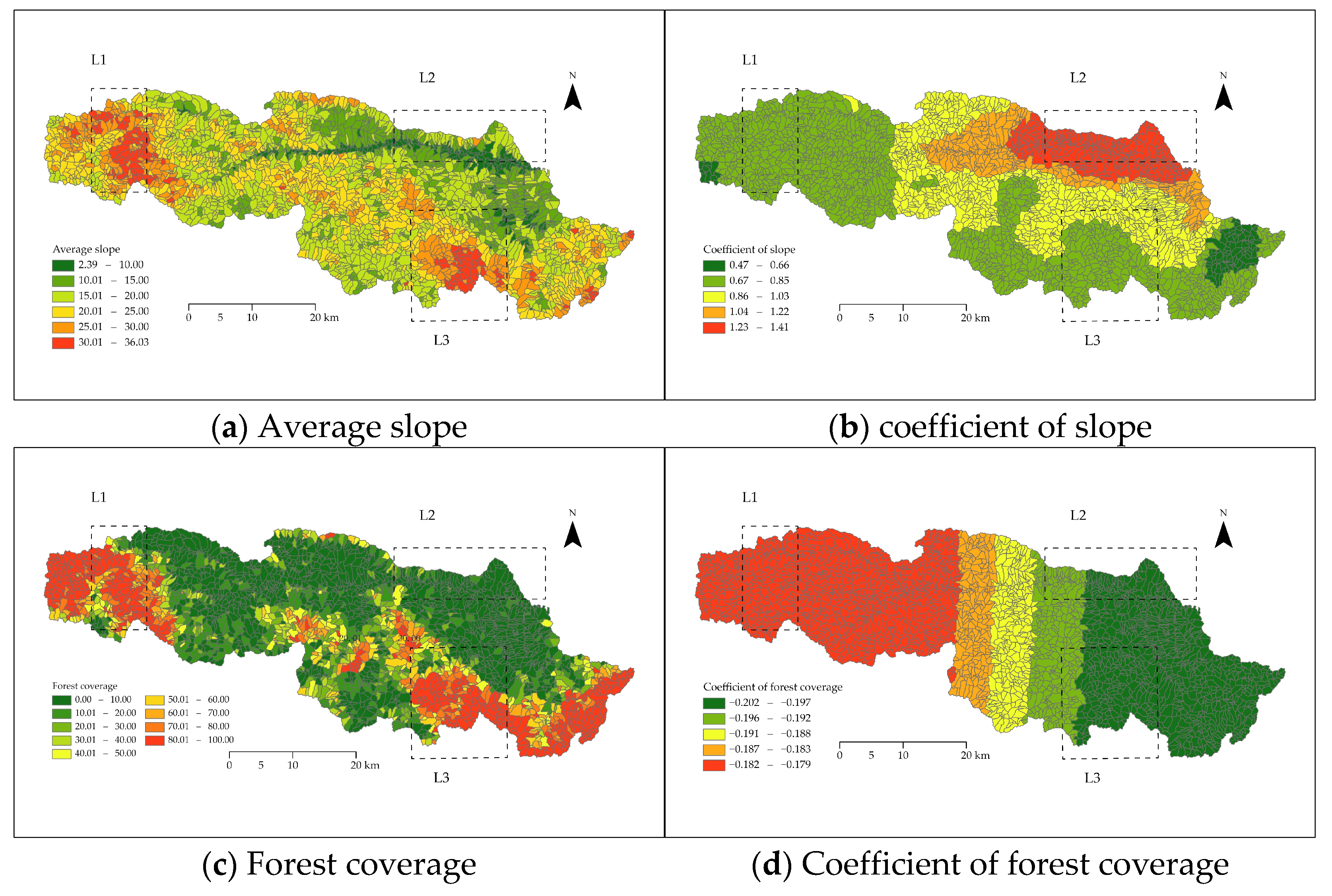
The separate optimized bandwidths from MGWR provide intuitive interpretation on the scale at which different processes operate [36]. The fixed bandwidth of GWR was 61 which meant there were 61 nearest neighbors involved in the calibration of the estimate. Likewise, the flexible bandwidths of MGWR descended in the order of forest coverage, grass coverage, average slope, and intercept, with the values being 2436, 885, 119, and 43, respectively. The lower the bandwidth is, the more frequently variables change. The optimal bandwidths revealed the influence of forest coverage was effectively stationary over space, and the influence of average slope was highly heterogenetic except for intercept. The bandwidth of MGWR was in the same order with effective number of parameters, too. The variation of bandwidths was connected in the spatial non-stationarity distribution; for example, the forest was concentrated in the west and south of Jihe basin, with variation being smooth while the slope changed sharply with the bandwidth being lower, shown in Figure 4. Contrary to global estimate of variables of OLS, GWR, and MGWR model provided individual estimate of variables in each hillslope, aggregated in Table 6.
Generally, forest and grass coverage had negative impacts on sediment modulus while average slope had positive impacts, shown in Table 6 of GWR and MGWR. MGWR results indicated the impact of variables on erosion was consistent with the descending order of parameter estimate, where the average coefficient of slope, grass coverage, and forest coverage were 0.90, −0.11, and −0.19 respectively. The coefficient revealed slope was the dominant factor, and the forest had more potentiality to weaken erosion than grass at the watershed scale.
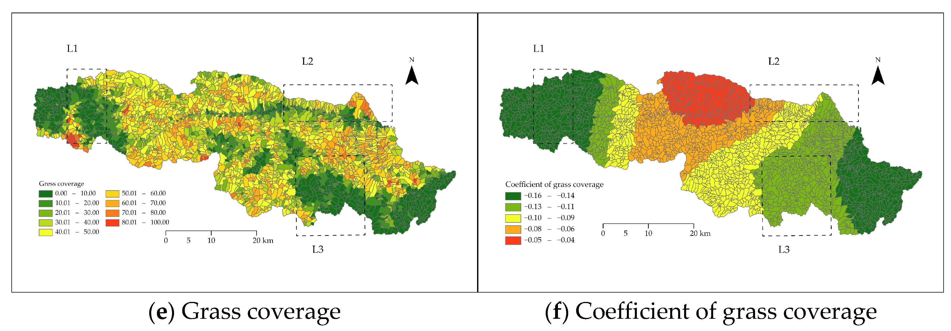
Additionally, the parameter estimates in each hillslope were shown in Figure 4. The parameter estimates of variables varied in hillslopes at the catchment, which indicated the coupling impacts on sediment modulus. As shown in Figure 4a,b, average slope of hillslope in L1 and L3 were high, while the coefficient was low, which meant the impact of steep slope on erosion was weakened. Figure 4d,f showed there were higher coefficient of grass coverage in L1 and higher coefficient of forest coverage in L3; it could be concluded that the high vegetation coverage in L1 and L3 weakened the erosion caused by steep hillslope. This could be confirmed in L2 that gentle hillslope with low vegetation coverage had the higher coefficient of average.
4. Discussion
The regression of MGWR at the catchment scales indicated the slope was the dominant factor affecting soil erosion at the catchment scales and forest cover has the power the power to reduce sediment more than grass (Table 6). The influence of factors operates in scales, where the influence of average slope was highly heterogenetic, and the influence of forest coverage was effectively stationary over space, revealed by bandwidth and effective number of parameters, shown in Table 6 and Figure 4. Besides, the erodible capability of steep slope was effectively weakened by high vegetation coverage. The result is also reached by the finding in Yimeng mountainous that slope-factor is the most factors affecting the distribution of soil erosion at a large-scale region and exhibited a decreasing trend with the vegetation reconstruction of Grain for Green Program [14]. Vegetation and topography factors have coupled effects on erosion operating at different scales [20], as evidenced by the bandwidths and regression coefficients of MGWR (Table 6).
The clustered and heterogeneous spatial distribution of influential factors has been a noteworthy issue of studying soil erosion at the catchment scales. Table 3 indicated the controversial distribution of sediment in hillslope of different vegetation cover and slope degree, where sediment modulus increases with the increase of vegetation coverage while it is well-known that sediment modulus increases with the increase of slope. The simulation results of soil erosion were revealed by the negative correlation of both forest and grass coverage, and the positive correlation of average slope in MGWR. Figure 4 (L1,L3) and Table 1 demonstrated a vital reason accounting for the controversial distribution, where hillslopes with high vegetation coverage were consistent with that with high slope in the spatial distribution and sediment modulus of different vegetation coverage under certain slope was similar. Therefore, the spatial correlation between slope and vegetation coverage accounted for the confused result of Table 3.
MGWR, a novel geographic analysis method, has substantial improvements compared to OLS and GWR [58,59]: (1) the flexible bandwidth yields a more realistic and useful spatial process model exhibiting the coupling impacts; (2) the specific bandwidth of each variable might be used as an indicator of the spatial scale of action of each spatial process. Limited to the availability of data and knowledge, three influential factors were used to study soil erosion at the catchment scales and more topography and vegetation factors could be considered, such as slope length and carbon emission.
The simulation results of RSEM provided detailed erosion distribution at both hillslopes scale and pixel scale, which most erosion models cannot provide. The validation of existing models is mostly based on export values of the outlet of basin, but less on spatial distribution of simulation results [31]. The volume of simulated sediment transport was consistent with the measured data in Table 2. Besides, the spatial pattern of soil erosion was agreement with other studies [60,61], which verified the soil erosion patten of RESM. This model simulation results would help understand the spatial distribution characteristics of erosion, prompt the reasons behind the occurrence of erosion, and evaluate the impact of these distributions at a large scale.
However, there are limitations to this model, as more factors about erosion should be taken into consideration, and the applicability of the model in other areas of the Loess Plateau needs to be improved. The simulation results were closed to the measured sediment, which were slightly larger than the real data because the RSEM have not taken several erosion reduction processes into simulation, such as check dam, etc. [32]. Both landscape engineering, terracing, the construction of check dams and reservoirs, and large-scale vegetation restoration projects were the primary factors driving reduction of sediment load [62]. The erosion reduction effects of check dams and others were not added into RSEM model, which made the simulation results unclear to some extent.
5. Conclusions
This study simulated soil erosion and sediment yield in Jihe Basin by the RSEM model in which measured hydrological data was calibrated, and used OLS, GWR, and MGWR to demonstrate the spatial distribution characteristics of erosion and its influential factors. The main goal of the current study was to determine the spatial heterogeneous relationship between soil erosion and influential factors. With the application of RSEM model, soil erosion, and sediment generation at the hillslope and watershed scale were simulated and displayed in the raster surface, providing a visible insight into the spatial distribution of erodibility of influential factors.
Simulated soil erosion of distributed physical genesis models provided detailed description and simulated data sources at the large scale, so that further study would be broader on soil erosion at the large-scale watershed. When confronting erosion distribution with spatial autocorrelation, spatial heterogeneity, and spatial stratified heterogeneity at a large scale, geographical analysis methods would perform better than traditional statistical methods. MGWR results promoted the goodness of fit and interpretability of variables that indicated how vegetation and topography factors operated in individual scale. Moreover, statistical analysis of MGWR would be helpful in the improvement of water and soil conservation management and region soil erosion model. For example, the steep slope area (i.e., L2 in Figure 4) should not be disturbed and maintain high vegetation coverage so that soil erosion is weakened; vegetation restoration project has an additional spatial reference according to the variation of reduction sediment effect of forest and grass in MGWR. Although our research presented a case study of Jihe basin, it would be valuable when combining with the measured data or simulated data in Loess Plateau with MGWR to study soil erosion at the watershed scale.
Author Contributions
Conceptualization, Z.Y. and Y.Z.; methodology, Z.Y.; software, Z.Y.; validation, J.Y., B.W., L.Z. and P.X.; formal analysis, Y.Z.; resources, Z.Y.; data curation, Z.Y.; writing—original draft preparation, Y.Z.; writing—review and editing, Z.Y.; visualization, Y.Z. All authors have read and agreed to the published version of the manuscript.
Funding
This research was found by the National Natural Science Foundation of China (Grant number: U2243210), National Natural Science Foundation of China (grant number: 32101591) and National key research priorities program of China-Variation mechanism and trend prediction of water and sediment in the Yellow River Basin (grant number: 2016YFC0402402).
Institutional Review Board Statement
Not applicable.
Informed Consent Statement
Not applicable.
Data Availability Statement
Data sharing not applicable. No new data were created or analyzed in this study. Data sharing is not applicable to this article.
Conflicts of Interest
The authors declare no conflict of interest.
References
- Li, Q.; Yu, P.; Li, G.; Zhou, D.; Chen, X. Overlooking Soil Erosion Induces Underestimation of the Soil C Loss in Degraded Land. Quat. Int. 2014, 349, 287–290. [Google Scholar] [CrossRef]
- Saikawa, E.; Rigby, M.; Prinn, R.G. Global and Regional Emission Estimates for HCFC-22. Atmos. Chem. Phys. 2012, 12, 10033–10050, Erratum in Atmos. Chem. Phys. 2014, 14, 4857–4858. [Google Scholar] [CrossRef] [Green Version]
- Zhengli, Y. A Summary on the History and Research Progress of Ecological Construction in the Loess Plateau. World For. Res. 2003, 16, 36–40. [Google Scholar]
- Wu, Y.; Liu, S. Modeling of Land Use and Reservoir Effects on Nonpoint Source Pollution in a Highly Agricultural Basin. J. Environ. Monit. Jem. 2012, 14, 2350–2361. [Google Scholar] [CrossRef]
- Trimble, S.W.; Crosson, P.U.S. Soil Erosion Rates-Myth and Reality. Science 2000, 289, 248–250. [Google Scholar] [CrossRef] [Green Version]
- Quinton, J.N.; Govers, G.; Van Oost, K.; Bardgett, R.D. The Impact of Agricultural Soil Erosion on Biogeochemical Cycling. Nat. Geosci. 2010, 3, 311–314. [Google Scholar] [CrossRef] [Green Version]
- Tang, K.L.; Zhang, K.L.; Liu, Y.B.; Wang, B.K.; Zha, X. Manmade Accelerated Erosion on the Loess Plateau and Global Change. J. Soil Water Conserv. 1992, 6, 88–96. [Google Scholar]
- Han, F.P.; Zhang, X.C.; Wang, Y.Q. The Estimation on Loading of Non-Point Source Pollution (N, P) in Different Watersheds of Yellow River. Acta Sci. Circumst. 2006, 26, 1893. [Google Scholar]
- Baoyuan, L. Temporal and Spatial Map of Water and Sediment of the Yellow River; Science Press: Beijing, China, 1993. [Google Scholar]
- Hua, F.; Wang, X.; Zheng, X.; Fisher, B.; Wang, L.; Zhu, J.; Tang, Y.; Yu, D.W.; Wilcove, D.S. Opportunities for Biodiversity Gains under the World’s Largest Reforestation Programme. Nat. Commun. 2016, 7, 12717. [Google Scholar] [CrossRef] [Green Version]
- Jia, X.; Fu, B.; Feng, X.; Hou, G.; Liu, Y.; Wang, X. The Tradeoff and Synergy between Ecosystem Services in the Grain-for-Green Areas in Northern Shaanxi, China. Ecol. Indic. 2014, 43, 103–113. [Google Scholar] [CrossRef]
- Jiongxin, X. Runoff and sediment variations in the upper reaches of Changjiang River and its tributaries due to deforestation. J. Hydrol. Eng. 2000, 1, 72–80. [Google Scholar] [CrossRef]
- Dachuan, R.; Liyi, Z.; Zhiping, Z.; Quanhua, L. A quantitative study on the effect of soil and water conservation measures on slope rill erosion mitigation with different scale in the Loess Plateau. J. Hydrol. Eng. 2010, 41, 1135–1141. [Google Scholar] [CrossRef]
- Qian, M.; Yu, X.; Lü, G.; Liu, Q. The Changing Relationship between Spatial Pattern of Soil Erosion Risk and Its Influencing Factors in Yimeng Mountainous Area, China 1986–2005. Environ. Earth Sci. 2012, 66, 1535–1546. [Google Scholar] [CrossRef]
- Zhao, J.; Feng, X.; Deng, L.; Yang, Y.; Zhao, Z.; Zhao, P.; Peng, C.; Fu, B. Quantifying the Effects of Vegetation Restorations on the Soil Erosion Export and Nutrient Loss on the Loess Plateau. Front. Plant Sci. 2020, 11, 573126. [Google Scholar] [CrossRef]
- Ran, Q.; Su, D.; Peng, L.; He, Z. Experimental Study of the Impact of Rainfall Characteristics on Runoff Generation and Soil Erosion. J. Hydrol. 2012, 424–425, 99–111. [Google Scholar] [CrossRef]
- Nadal-Romero, E.; Lasanta, T.; García-Ruiz, J.M. Runoff and Sediment Yield from Land under Various Uses in a Mediterranean Mountain Area: Long-Term Results from an Experimental Station. Earth Surf. Processes Landf. 2013, 38, 346–355. [Google Scholar] [CrossRef]
- Defersha, M.B.; Melesse, A.M. Effect of Rainfall Intensity, Slope and Antecedent Moisture Content on Sediment Concentration and Sediment Enrichment Ratio. Catena 2012, 90, 47–52. [Google Scholar] [CrossRef]
- Xiao, P.; Yao, W.; Römkens, M.; Rernkens, J. Effects of Grass and Shrub Cover on the Critical Unit Stream Power in Overland Flow. Int. J. Sediment Res. 2011, 26, 8. [Google Scholar] [CrossRef]
- Wei, Q.; Wenhong, C.; Changqing, Z. Review on the coupling influences of vegetation and topography to soil erosion and sediment yield. J. Sediment Res. 2015, 3, 74–80. [Google Scholar] [CrossRef]
- Carroll, C.; Halpin, M.; Burger, P.; Bell, K.; Sallaway, M.M.; Yule, D.F. The Effect of Crop Type, Crop Rotation, and Tillage Practice on Runoff and Soil Loss on a Vertisol in Central Queensland. Aust. J. Soil Res. 1997, 35, 925–939. [Google Scholar] [CrossRef]
- Hongbo, W.; Rui, L.; Qinke, Y. Research Advances of Vegetation Effect on Soil and Water Conservation in China. Acta Phytoecol. Sin. 2002, 4, 489–496. [Google Scholar]
- Guanghui, Z. Research situation and prospect of the soil erosion model. Adv. Water Sci. 2002, 3, 389–396. [Google Scholar] [CrossRef]
- Pandey, S.; Kumar, P.; Zlatic, M.; Nautiyal, R.; Panwar, V.P. Recent Advances in Assessment of Soil Erosion Vulnerability in a Watershed. Int. Soil Water Conserv. Res. 2021, 9, 14. [Google Scholar] [CrossRef]
- Pandey, A.; Mathur, A.; Mishra, S.K.; Mal, B.C. Soil Erosion Modeling of a Himalayan Watershed Using RS and GIS. Environ. Geol. 2009, 59, 399–410. [Google Scholar] [CrossRef]
- Laflen, J.M.; Elliot, W.J. WEPP-Predicting Water Erosion Using a Process-Based Model. J. Soil Water Conserv. 1997, 52, 96–102. [Google Scholar]
- Obeta, I.N.; Adewumi, J.K. Soil Loss in Samaru Zaria Nigeria: A Comparison of Wepp and Eurosem Models. Niger. J. Technol. 2013, 32, 123586. [Google Scholar]
- Kirkby, M. Modelling Erosion—The PESERA Project; The First SCAPE Workshop: Alicante, Spain, 2003. [Google Scholar]
- Fernández, C.; Vega, J.A. Evaluation of RUSLE and PESERA Models for Predicting Soil Erosion Losses in the First Year after Wildfire in NW Spain. Geoderma 2016, 273, 64–72. [Google Scholar] [CrossRef]
- Sadeghi, S.H.; Gholami, L.; Darvishan, A.K.; Saeidi, P. A Review of the Application of the MUSLE Model Worldwide. Hydrol. Sci. J. J. Des Sci. Hydrol. 2014, 59, 365–375. [Google Scholar] [CrossRef] [Green Version]
- Xingmin, M.; Pengfei, L.; Peng, G.; Guangju, Z.; Wenyi, S. Review and evaluation of soil erosion models applied to China loess plateau. Yellow River 2016, 38, 100–110+114. [Google Scholar]
- Zhihong, Y. Simulation of Soil and Water Loss Process at Regional Scale Based on GIS. Ph.D. Thesis, University of Chinese Academy of Sciences, Beijing, China, 2010. [Google Scholar]
- Jinfeng, W.; Yilan, L.; Xin, L. Spatial Data Analysis Tutorial; Science Press: Beijing, China, 2010. [Google Scholar]
- Binbin, L.; Yong, G.; Kun, Q.; Huangjiang, Z. A review on geographically weighted regression. Geomat. Inf. Sci. Wuhan Univ. 2020, 45, 1356–1366. [Google Scholar] [CrossRef]
- Fotheringham, A.; Brunsdon, C.; Charlton, M. Geographically Weighted Regression: The Analysis of Spatially Varying Relationships; John Wiley Sons: Hoboken, NJ, USA, 2002; pp. 554–556. [Google Scholar]
- Oshan, T.M.; Li, Z.; Kang, W.; Wolf, L.J.; Fotheringham, A.S. MGWR: A Python Implementation of Multiscale Geographically Weighted Regression for Investigating Process Spatial Heterogeneity and Scale. Int. J. Geo-Inf. 2019, 8, 269. [Google Scholar] [CrossRef] [Green Version]
- Goodchild, M.F. Metrics of scale in remote sensing and GIS. Int. J. Appl. Earth Obs. Geoinf. 2001, 3, 114–120. [Google Scholar] [CrossRef]
- Fotheringham, A.T.; Yang, W.; Kang, W. Multiscale Geographically Weighted Regression (MGWR). Ann. Am. Assoc. Geogr. 2017, 107, 1247–1265. [Google Scholar] [CrossRef]
- Yu, H.; Fotheringham, A.S.; Li, Z.; Oshan, T.; Kang, W.; Wolf, L.J. Inference in Multiscale Geographically Weighted Regression. Geogr. Anal. 2020, 52, 87–106. [Google Scholar] [CrossRef]
- Qingyun, L.; Yanwei, S.; Xinxiao, Y.; Fan, W. Changes of sediment yield in Jihe watershed on Loess Plateau in past 50 years. J. Sediment Res. 2014, 2, 44–48. [Google Scholar] [CrossRef]
- Ruijie, Q.; Guifang, L.; Ping, L. Impacts of Precipitation and Land Use Change on runoff and Sediment in Luoyugou Watershed. J. Soil Water Conserv. 2018, 32, 29–34+40. [Google Scholar] [CrossRef]
- Wenpin, D.; Haiguang, L.; Xinxiao, Y.; Yang, Z.; Henian, W.; Feng, X. Influence of the Change of Land Use/Land Cover and Precipitation Variationon Runoff and Sediment Transport in Lüergou River Watershed on the Loess Plateau. Res. Soil Water Conversat. 2011, 18, 226–231. [Google Scholar]
- Xizhi, L.; Lingling, K.; Zhonguo, Z.; Juan, S.; Yongxin, M. Characteristics of Slope Runoff under Different Vegetation Conditions in Lvergou Watershed of the Loess Plateau. Ecol. Environ. Sci. 2015, 24, 1113–1117. [Google Scholar] [CrossRef]
- Aston, A. Rainfall Interception by Eight Small Trees. J. Hydrol. 1979, 42, 383–396. [Google Scholar] [CrossRef]
- Von Hoyningen-Huene, J. Die Interzeption des Niederschlags in landwirtschaftlichen Pflanzenbeständen. Arbeitsbericht Deutscher Verband für Wasserwirtschaft und Kulturbau; DVWK: Braunschweig, Germany, 1981; Volume 63. [Google Scholar]
- Kostiakov, A.N. On the Dynamics of the Coefficient of Water-Percolation in Soils and on the Necessity of Studying It from a Dynamic Point of View for Purposes of Amelioration. Trans. 6th Comm. Int. Soc. Soil Sci. Russ. 1932, 14, 17–21. [Google Scholar]
- Kamphorst, E.C.; Jetten, V.; Guerif, J.; Iversen, B.V.; Paz, A. Predicting Depressional Storage from Soil Surface Roughness. Soil Sci. Soc. Am. J. 2000, 64, 1749–1758. [Google Scholar] [CrossRef]
- Govers, G.; Wallings, D.E.; Yair, A.; Berkowicz, S. Empirical Relationships for the Transport Capacity of Overland Flow. IAHS Publ. 1990, 189, 45–63. [Google Scholar]
- Smith, R.E.; Goodrich, D.C.; Quinton, J.N. Dynamic, Distributed Simulation of Watershed Erosion: The KINEROS2 and EUROSEM Models. J. Soil Water Conserv. 1995, 50, 517–520. [Google Scholar]
- De Roo, A.P.J.; Wesseling, C.G.; Ritsema, C.J. Lisem: A Single-Event Physically Based Hydrological and Soil Erosion Model for Drainage Basins. I: Theory, Input and Output. Hydrol. Process. 1996, 10, 1107–1117. [Google Scholar] [CrossRef]
- Morgan, R.P.C.; Quinton, J.N.; Smith, R.E.; Govers, G.; Poesen, J.W.A.; Auerswald, K.; Chisci, G.; Torri, D.; Styczen, M.E. The European Soil Erosion Model (EUROSEM): A Dynamic Approach for Predicting Sediment Transport from Fields and Small Catchments. Earth Surf. Processes Landf. 1998, 23, 527–544. [Google Scholar] [CrossRef]
- Coulson, M.; van Deursen, W.P.A.; Danson, F.M.; Plummer, S.E.; Williams, J.; Mather, P.M. Geographical Information Systems and Dynamic Models. Geogr. J. 1996, 162, 219. [Google Scholar] [CrossRef]
- Myneni, R.B.; Ramakrishna, R.; Nemani, R.; Running, S.W. Estimation of Global Leaf Area Index and Absorbed Par Using Radiative Transfer Models. IEEE Trans. Geosci. Remote Sens. 2002, 35, 1380–1393. [Google Scholar] [CrossRef] [Green Version]
- Xiaoming, Z.; Wenhong, C.; Lijun, Z. Progress review and discussion on sediment delivery ratio and its dependence on scale. Acta Sci. Circum. 2014, 34, 7475–7485. [Google Scholar] [CrossRef] [Green Version]
- Leiva, B.; Ramirez, O.A.; Schramski, J.R. A Framework to Consider Energy Transfers within Growth Theory. Energy 2019, 178, 624–630. [Google Scholar] [CrossRef]
- Yang, W.; Fotheringham, A.; Harris, P. An Extension of Geographically Weighted Regression with Flexible Bandwidths; GISRUK: Lancaster, UK, 2012. [Google Scholar]
- Wang, W.; Jiao, J.; Hao, X. Study on Rainfall Erosivity in China. J. Soil Water Conserv. 1995, 9, 5–18. [Google Scholar]
- Zhou, Z.; Cheng, X. Spatial heterogeneity of influencing factors of PM2.5 in Chinese cities based on MGWR model. China Environ. Sci. 2021, 41, 2552–2561. [Google Scholar] [CrossRef]
- Tiyan, S.; Haochen, Y.; Lin, Z.; Hengyu, G.; Honghao, H. On Hedonic Price of Second-Hand Houses in Beijing Based on Multi-Scale Geographically Weighted Regression: Scale Law of Spatial Heterogeneity. Econ. Geogr. 2020, 40, 75–83. [Google Scholar] [CrossRef]
- Wang, N.; Yao, Z.; Liu, W.; Lv, X.; Ma, M. Spatial Variabilities of Runoff Erosion and Different Underlying Surfaces in the Xihe River Basin. Water 2019, 11, 352. [Google Scholar] [CrossRef] [Green Version]
- Guo, S.; Zhu, Z.; Lyu, L. Effects of Climate Change and Human Activities on Soil Erosion in the Xihe River Basin, China. Water 2018, 10, 1085. [Google Scholar] [CrossRef] [Green Version]
- Wang, S.; Fu, B.; Piao, S.; Lü, Y.; Ciais, P.; Feng, X.; Wang, Y. Reduced Sediment Transport in the Yellow River Due to Anthropogenic Changes. Nat. Geosci. 2015, 9, 38–41. [Google Scholar] [CrossRef]
Figure 1.
The location of Jihe Basin.

Figure 2.
Daily precipitation, runoff and sediment load in 2015.

Figure 3.
The framework of RSEM.

Figure 4.
The distribution of influential factors and their coefficients in hillslopes of Jihe Basin. (a): Average slope in hillslopes; (b): Coefficient of slope in the MGWR results; (c): Forest coverage in hillslopes; (d): Coefficient of forest coverage in the MGWR results; (e): Grass coverage in hillslopes; (f): Coefficient of grass coverage in the MGWR results.


Table 1.
The areas (Km2) in different slope (°) and vegetation coverage (%) of hillslopes.
| Vegetation Coverage (%) | ||||||||||
|---|---|---|---|---|---|---|---|---|---|---|
| 0–10 | 10–20 | 20–30 | 30–40 | 40–50 | 50–0 | 60–70 | 70–100 | Sum | ||
| Average Slope (°) | 0–10 | 20.08 | 14.97 | 12.16 | 15.62 | 6.67 | 5.25 | 1.31 | 0.73 | 76.77 |
| 10–15 | 1.55 | 2.64 | 12.36 | 21.28 | 71.10 | 71.60 | 65.17 | 15.00 | 260.70 | |
| 15–20 | 0.11 | 1.13 | 4.27 | 26.46 | 72.68 | 159.62 | 211.78 | 164.94 | 640.97 | |
| 20–25 | 0.00 | 0.50 | 0.75 | 6.15 | 28.56 | 44.51 | 109.32 | 293.57 | 483.34 | |
| 25–30 | 0.00 | 0.00 | 0.64 | 1.31 | 3.70 | 5.79 | 29.88 | 195.18 | 236.49 | |
| 30–70 | 0.00 | 0.00 | 0.00 | 0.00 | 0.24 | 0.44 | 3.76 | 90.14 | 94.58 | |
| sum | 21.75 | 19.24 | 30.18 | 70.81 | 182.94 | 287.20 | 421.21 | 759.54 | ||
Table 2.
Simulation results of sediment volume.
| Month | Average Precipitation (mm) | Measured Sediment Volume (Kg) | Adjusted Sediment Volume (Kg) | Simulated Sediment Volume (Kg) |
|---|---|---|---|---|
| 4 | 85.5 | 2.74 × 10⁷ | 4.93 × 10⁷ | 7.30 × 10⁷ |
| 6 | 126 | 7.19 × 10⁶ | 1.29 × 10⁷ | 4.63 × 10⁷ |
Table 3.
Sediment modulus in hillslopes of different vegetation coverage and slope degree (Kg/Km2·a).
Table 3.
Sediment modulus in hillslopes of different vegetation coverage and slope degree (Kg/Km2·a).
| Vegetation Coverage (%) | ||||||||||
|---|---|---|---|---|---|---|---|---|---|---|
| 0–10 | 10–20 | 20–30 | 30–40 | 40–50 | 50–60 | 60–70 | 70–100 | Average | ||
| Slope (°) | 0–10 | 22,857 | 23,534 | 26,225 | 22,731 | 28,200 | 29,948 | 28,590 | 28,151 | 24,587 |
| 10–15 | 37,924 | 35,260 | 33,845 | 36,427 | 35,219 | 35,263 | 34,637 | 35,495 | 35,150 | |
| 15–20 | 37,176 | 38,301 | 37,665 | 39,983 | 39,238 | 39,183 | 39,083 | 39,274 | 39,158 | |
| 20–25 | 0 | 45,565 | 48,618 | 45,217 | 43,691 | 44,191 | 44,016 | 43,626 | 43,838 | |
| 25–30 | 0 | 0 | 48,456 | 49,551 | 48,364 | 49,712 | 49,732 | 49,139 | 49,331 | |
| 30–70 | 0 | 0 | 49,644 | 50,006 | 53,942 | 53,305 | 0 | 0 | 53,297 | |
| Average | 24,007 | 26,580 | 31,993 | 35,740 | 38,167 | 39,042 | 40,531 | 45,071 | 41,301 | |
Table 4.
Comparison of OLS, GWR and MGWR results.
| OLS | GWR | MGWR | |
|---|---|---|---|
| R2 | 0.87 | 0.94 | 0.93 |
| Adjust R2 | 0.87 | 0.93 | 0.92 |
| AICc | 2158.01 | 1119.36 | 1160.55 |
| Residual sum of squares | 351.24 | 171.95 | 204.79 |
| Effective number of parameters | 394.69 | 223.20 | |
Table 5.
t-test of variables in OLS, GWR and MGWR.
| t-Test | OLS | GWR | MGWR |
|---|---|---|---|
| Forest Coverage | 0.00 | non-significant | significant |
| Grass Coverage | 0.51 | non-significant | significant |
| Average Slope | 0.00 | partial significant | significant |
Table 6.
Parameter estimation of OLS, GWR and MGWR.
| Variable | OLS | GWR | MGWR | ||||||||
|---|---|---|---|---|---|---|---|---|---|---|---|
| Bandwidth | Mean | Std | Min | Max | Bandwidth | Mean | Std | Min | Max | ||
| Forest Coverage | −0.05 | 61 | −0.28 | 0.50 | −3.10 | 1.13 | 2436 | −0.19 | 0.01 | −0.20 | −0.18 |
| Grass Coverage | 0.01 | 61 | −0.16 | 0.27 | −1.82 | 0.72 | 885 | −0.11 | 0.03 | −0.16 | −0.04 |
| Average Slope | 0.97 | 61 | 0.89 | 0.25 | 0.12 | 1.86 | 119 | 0.90 | 0.19 | 0.47 | 1.41 |
| Intercept | 0.00 | 61 | 0.08 | 0.41 | −2.26 | 1.54 | 43 | 0.10 | 0.18 | −0.28 | 0.62 |
Publisher’s Note: MDPI stays neutral with regard to jurisdictional claims in published maps and institutional affiliations. |
© 2022 by the authors. Licensee MDPI, Basel, Switzerland. This article is an open access article distributed under the terms and conditions of the Creative Commons Attribution (CC BY) license (https://creativecommons.org/licenses/by/4.0/).
Share and Cite
MDPI and ACS Style
Yao, Z.; Zhang, Y.; Xiao, P.; Zhang, L.; Wang, B.; Yang, J. Soil Erosion Process Simulation and Factor Analysis of Jihe Basin. Sustainability 2022, 14, 8114. https://doi.org/10.3390/su14138114
AMA Style
Yao Z, Zhang Y, Xiao P, Zhang L, Wang B, Yang J. Soil Erosion Process Simulation and Factor Analysis of Jihe Basin. Sustainability. 2022; 14(13):8114. https://doi.org/10.3390/su14138114
Chicago/Turabian StyleYao, Zhihong, Yu Zhang, Peiqing Xiao, Lu Zhang, Bo Wang, and Jianchen Yang. 2022. "Soil Erosion Process Simulation and Factor Analysis of Jihe Basin" Sustainability 14, no. 13: 8114. https://doi.org/10.3390/su14138114
Note that from the first issue of 2016, this journal uses article numbers instead of page numbers. See further details here.